Trapped-ion Fock state preparation by potential deformation

Abstract

We propose protocols to prepare highly excited energy eigenstates of a trapped ion in a harmonic trap which do not require laser pulses to induce transitions among internal levels. Instead the protocols rely on smoothly deforming the trapping potential between single and double well configurations. The speed of the changes is set to minimize non-adiabatic transitions by keeping the adiabaticity parameter constant. High fidelities are found for times more than two orders of magnitude smaller than with linear ramps of the control parameter. Deformation protocols are also devised to prepare superpositions to optimize interferometric sensitivity, combining the ground state and a highly excited state.

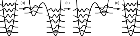
Figure 1: Scheme for Fock-state preparation. (a) Demultiplexing: splitting the harmonic trap into an asymmetrical double well; (b) Bias inversion of the double well; (c) Multiplexing: inverse of demultiplexing. The shaded wave functions are the ideal initial and target states.

Introduction. A trapped-ion architecture for quantum technologies rests on combining basic operations such as logic gates or shuttling, and generally needs controlling quickly and accurately internal and motional states. Preparing (Fock) states with a well defined number of vibrational quanta is one of the basic manipulations that may be used to implement quantum memories, entanglement operations, or communications Martínez-Garaot et al. (2013); Galland et al. (2014). Fock states with large number of phonons can be useful in metrology protocols based on NOON states, which give measurement outcomes with uncertainties reaching the Heisenberg bound Zhang et al. (2018); Giovannetti et al. (2011). Also, superpositions of eigenstates with maximally separated energies give optimal interferometric sensitivities Margolus and Levitin (1998); Caves and Shaji (2010) e.g. to measure motional frequency changes McCormick et al. (2019). Several schemes to prepare Fock states have been proposed Cirac et al. (1993, 1994); Meekhof et al. (1996); Davidovich et al. (1996); de Matos Filho and Vogel (1996); Abah et al. (2019), but for a trapped ion they have only been produced by sequences of Rabi pulses, which is in fact quite challenging, as an $n$-phonon state needs of the order of $n$ pulses with accurately defined frequency and area, so the errors in intensity and frequency, and timing imperfections reduce the fidelity Linington et al. (2008). A recent experiment McCormick et al. (2019) applied such sequences of Rabi pulses with unprecedented accuracy to approximately reach Fock states of up to $n=100$. To reach the highest Fock states, higher order sidebands, i.e., pulses that jump more than a single level at a time (up to four in this case), had to be applied, but still the required time and errors grow rapidly with the phonon number.

The goal pursued here is to create an excited Fock state for a single ion from the ground state without laser-induced internal transitions involved, by means of deformations of the trap. The potentials in linear, multielectrode Paul ion traps can be deformed by programming the voltages applied to the electrodes, see Kaufmann et al. (2014); Home and Steane (2006); Nizamani and Hensinger (2012); Fürst et al. (2014). Since these operations only require that the trapped particle has an electrical charge they can be applied to other particles besides ions, like nano-particles Guan et al. (2011) or electrons Segal and Shapiro (2006). Operations that do not use lasers to link internal and motional states are worth exploring for quantum technologies since they would allow to create universal control devices independent of the internal structure of the atom, and free from the usual disadvantages of laser control (frequency, position and intensity instabilities, spontaneous decay) although, of course, they involve their own technical limitations and mass dependence. The present proposal intends to demonstrate some possible benefits of the strategy based on trap deformations and motivate further work to test and overcome these limitations.

The approach proposed here is depicted in Fig. 1 and involves three steps: (a) demultiplexing; (b) bias inversion; (c) multiplexing. Steps (a) and (c) could be carried out adiabatically or using some shortcut to adiabaticity (STA) Torrontegui et al. (2013); Guéry-Odelin et al. (2019) since the level ordering at the start and at the end of the process is conserved. For the second step the ordering of the levels is altered, so there is no global adiabatic mapping that connects initial and final states. However, in a fast process the wells are effectively independent so that STA approaches can also be applied as demonstrated in Martínez-Garaot et al. (2015). A faster-than-adiabatic approach for step (a) was applied in Martínez-Garaot et al. (2013) with neutral atoms, but only for a two motional-level model. In this paper we design step (c) using an STA approach to minimize the non-adiabatic transitions distributing them homogeneously along the process time Martínez-Garaot et al. (2015); Palmero et al. (2019). The first step requires a similar protocol but in reverse.

Multiplexing. Consider a single ion in a trap which is effectively one dimensional driven by the Hamiltonian

$$H(t)=\frac{p^{2}}{2M}+\alpha(t)x^{2}+\beta(t)x^{4}+\gamma(t)x,$$ (1)

where $x$, $p$ are the position and momentum operators, and $M$ the mass of the ion; $\alpha(t)$, $\beta(t)$ and $\gamma(t)$ are in principle time-dependent coefficients.

The trapping potential $V_{t}(x)=\alpha(t)x^{2}+\beta(t)x^{4}+\gamma(t)x$ is a double well potential when $\alpha(t)<0$ and $\beta(t)>0$. The term $\gamma(t)x$ corresponds to a homogeneous electric field that induces an energy bias between the wells. In the symmetric potential ($\gamma=0$) the minima are at $x_{0,\pm}=\pm\sqrt{-{\alpha}/{(2\beta)}}$. We consider the bias small enough so that the shift of the minima depends linearly on $\gamma$. The positions of the minima for a non-zero small bias are Martínez-Garaot et al. (2015) $x_{0,\pm}\approx\pm\sqrt{-{\alpha}/({2\beta})}+{\gamma}/({4\alpha}),$ valid when $\absolutevalue{\gamma}\ll{4\sqrt{2}}\sqrt{-{\alpha^{3}}/{\beta}}/3,$ which defines the small-bias regime. In this regime the energy difference between the wells is approximately $\Delta V_{t}=\gamma D$, where $D\equiv x_{0,+}-x_{0,-}=\sqrt{-{2\alpha}/{\beta}}$ is the distance between the minima. The parameters for the initial double well will be chosen within this regime. The effective frequency $\omega_{eff,\pm}$ of each well, in the small-bias regime is $\omega_{eff,\pm}\approx\Omega=2\sqrt{{-\alpha}/{M}}$.

When $\alpha>0$ and $\beta=0$ the trapping potential is harmonic with angular frequency $\omega=\sqrt{{2\alpha}/{M}}$. Multiplexing consists on driving the system from the double well configuration to the harmonic trap configuration so that the initial eigenstates are dynamically mapped onto the final ones. For simplicity we shall keep $\gamma(t)$ fixed, $\gamma(t)=\gamma$. The boundary conditions in a multiplexing operation are $\alpha_{0}<0$, $\beta_{0}>0$ for the initial values and $\alpha_{f}>0$, $\beta_{f}=0$ for the final values,

$$\begin{split}V_{t=0}\left(x\right)&=\alpha_{0}x^{2}+\beta_{0}x^{4}+\gamma x,\\ V_{t=t_{f}}\left(x\right)&=\alpha_{f}\left(x-x_{eq}\right)^{2}-{\gamma}/({4\alpha_{f}^{2}}),\end{split}$$ (2)

with $x_{eq}\equiv-{\gamma}/({2\alpha_{f}})$. We shall also impose that the frequency of the final harmonic trap is equal to the frequency of the initial wells so $\alpha_{f}=2\absolutevalue{\alpha_{0}}$. If the evolution is adiabatic, the lowest state of the upper well ($n$th state globally) will become the $n$th Fock excited state $\ket{n}$ of the final harmonic potential. If the wells are deep enough, in the left (right) well there is a set of harmonic eigenstates $\ket{n_{L}}$ ($\ket{n_{R}}$) with energies $E_{n_{L}}=\hbar\Omega_{0}(n_{L}+1/2)$ $\left(E_{n_{R}}=\hbar\Omega_{0}(n_{R}+1/2)+\Delta V_{t}\right)$, where $\Omega_{0}\equiv 2\sqrt{{-\alpha_{0}}/{m}}$. We need the initial ground state of the right well, $\ket{0_{R}}$, to be the $n$th excited state of the whole system, so the inequality $E_{(n-1)_{L}}<E_{0_{R}}<E_{n_{L}}$ must be satisfied,

$$n-1<{\gamma D_{0}}/{(\hbar\Omega_{0})}<n,$$ (3)

where $D_{0}\equiv D(\alpha_{0},\beta_{0})$. The ratio ${D}/{\Omega}=\sqrt{{M}/({2\beta})}$ only depends on $\beta$ so a change of $\alpha$ within the small bias regime for constant $\beta$ does not modify this state ordering. In our simulations we choose the value $\gamma=(n-{1}/{2}){\hbar\Omega_{0}}/{D_{0}}$ for the bias. The small bias condition and Eq. (3) provide an upper bound for the highest Fock state that can be prepared with specific initial values of the control parameters $\alpha_{0}$ and $\beta_{0}$, $n\ll{4}\sqrt{-{M\alpha_{0}^{3}}/({\hbar^{2}\beta_{0}^{2}})}/3.$ To design the driving of the control parameters, a straightforward approach would be an adiabatic evolution, for example a linear ramp protocol along a large run-time. Long times, however, are inadequate for many applications and give rise to decoherence. Shortcuts to adiabaticity Torrontegui et al. (2013); Guéry-Odelin et al. (2019) stand out as a practical, faster option.

Design of the process. Shortcuts to adiabaticity Torrontegui et al. (2013); Guéry-Odelin et al. (2019) are a family of methods which speed up adiabatic processes to get the same final populations or states in shorter times. Shortcuts have been applied for many different systems and operations and can be adapted to be robust against implementation errors and noise Guéry-Odelin et al. (2019).

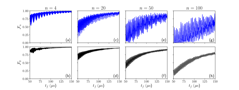
Figure 2: Preparation of Fock states $\ket{n}$ and superposition states $({\ket{0}+e^{i\varphi}\ket{n}})/{\sqrt{2}}$ using FAQUAD. The different columns show the results for the different values of $n$. Upper row: fidelity of the stated evolved by FAQUAD from the $n$th excited of the double well with respect to $\ket{n}$, the $n$th Fock state of the harmonic trap. Lower row: fidelity of the state evolved from the ground state with respect to $\ket{0}$ using the FAQUAD trap deformation designed to get $\ket{n}$. $\alpha_{0}=-4.7$ pN/m, $\alpha_{f}=-2\alpha_{0}=9.4$ pN/m, $\beta_{0}=0.052$ N/m³, $\beta_{f}=0$, $M(^{9}$Be${}^{+})=9.012$ a.u, $\epsilon=1$ pN/m, and $\kappa=100/(\alpha_{0}-\alpha_{f})=-7.092$ m/pN.

Among the different STA techniques available, Fast quasiadiabatic dynamics (FAQUAD) Martínez-Garaot et al. (2015) is well suited to our current objective. Invariants-based inverse engineering Chen et al. (2011) requires explicit knowledge of a dynamical invariant of the Hamiltonian, which is not available here, and Fast-Forward driving Masuda and Nakamura (2010); Torrontegui et al. (2012) produces potentials with singularities due to the nodes of the wave function Martínez-Garaot et al. (2016), which can be problematic with highly excited states. FAQUAD reduces the diabatic transitions between the states of the Hamiltonian by making the adiabaticity criterion constant during the process. For a time-dependent Hamiltonian that depends on a single control parameter $H(t)=H\left[\lambda(t)\right]$ such that $\lambda(t)$ is a monotonous function in the $\left[0,t_{f}\right]$ interval, the adiabaticity criterion to avoid transitions between the instantaneous eigenstates $\ket{n(\lambda)}$ and $\ket{m(\lambda)}$ is Schiff (1968)

$$\hbar\dot{\lambda}\;\absolutevalue{\frac{\matrixelement{n(\lambda)}{dH/d\lambda}{m(\lambda)}}{\left[E_{n}(\lambda)-E_{m}(\lambda)\right]^{2}}}=c\ll 1,$$ (4)

where $E_{n}(\lambda)$($E_{m}(\lambda)$) are the instantaneous eigenenergies and the dot stands for time derivative.

FAQUAD imposes a constant $c$, so Eq. (4) becomes a differential equation for $\lambda(t)$. The value of $c$ is determined by the boundary conditions $\lambda(0)$ and $\lambda(t_{f})$. Equation (4) implies that the control parameter evolves more slowly when the Hamiltonian changes rapidly with the control parameter and/or near avoided crossings.

We eliminate one degree of freedom in Eq. (1) by taking $\alpha$ as the master control parameter ($\alpha=\lambda$) and making $\beta=\beta(\alpha)$. Eq. (4) has to be solved with the boundary conditions for $\alpha$ and $\beta$. To choose $\beta(\alpha)$ we consider that the largest possible values of $\beta$ should hold while $\alpha$ changes sign so that the levels in the intermediate quartic well are not too close. A simple choice is to keep $\beta\approx\beta_{0}$ constant until $\alpha>0$ increases and the quadratic part dominates. Then we can let $\beta$ drop to zero without any significant effect. While $\beta$ is constant the energy difference between the wells in units of the instantaneous motional quantum $N_{q}={\gamma D}/({\hbar\Omega})={\gamma}\sqrt{{M}/{(2\beta)}}/\hbar,$ is constant. We choose for $\beta$ the form $\beta(\alpha)=a+b\;S\left[\kappa(\alpha-\epsilon)\right],$ where $S(x)=(1+e^{-x})^{-1}$ is the (sigmoid) logistic function. $\epsilon$ and $\kappa$ set the position and the width of the region where the parameter $\beta$ ramps from its initial to the final value. We choose $\epsilon>0$ so that $\beta\approx\beta_{0}$ around $\alpha=0$. A larger $\kappa$ implies a narrower jump. When $\kappa\gg max\{\left(\absolutevalue{\alpha_{0}}+\epsilon\right)^{-1},\left(\absolutevalue{\alpha_{f}}-\epsilon\right)^{-1}\}$ the ramp of $\beta$ is narrow enough so that when $\alpha$ goes to $\alpha_{0}$ ($\alpha_{f}$) $\beta$ goes asymptotically to $a$ ($a+b$) and then the boundary conditions demand that $a=-b=\beta_{0}$.

We choose $\alpha_{0}=-4.7$ pN/m, $\alpha_{f}=2\absolutevalue{\alpha_{0}}=9.4$ pN/m, $\beta_{0}=0.052$ N/m³, and ⁹Be⁺ ions in the numerical simulations. With the chosen $\alpha_{0}$, $\beta_{0}$ and the mass of ⁹Be⁺, $\Omega_{0}=2\pi\,\times\,5.6$ MHz and $D_{0}=13.45$ $\mu$m. For the ground state of the highest energy well to be the $n$th excited state of the full Hamiltonian, the bias is chosen as $\gamma=(n-0.5){\hbar\Omega_{0}}/{D_{0}}$.

Avoided level crossings occur at $\alpha<0$, near $\alpha=0$ in a critical region where the small bias condition fails and the double well becomes a single quartic well. The gap between the eigenstates near $\alpha=0$ is approximately proportional to $\beta^{1/3}$ Vranivcar and Robnik (2000). Thus, at $\alpha\approx 0$, $\beta$ should be as large as possible within experimental constraints.

Figure 3: Fidelity vs. final time for the creation of Fock states using a linear ramp of the control parameter $\alpha$: triangles, $n=20$; solid red line, $n=50$ and dashed blue line $n=100$. Same parameters as in Fig. 2.

In our multilevel scenario we modify Eq. (4) to Palmero et al. (2019) $c=\hbar\dot{\lambda}\sum_{m\neq n}\absolutevalue{\frac{\matrixelement{n(\lambda)}{{dH/}{d\lambda}}{m(\lambda)}}{\left[E_{n}(\lambda)-E_{m}(\lambda)\right]^{2}}},$ taking only the four closest eigenstates (two from below and two from above) of the relevant state in the sum. Note the shorthand notation $|n\rangle\equiv|n(\lambda_{f})\rangle$ for the eigenstates of the final harmonic oscillator.

Results. We have numerically solved the time-dependent Schrödinger equation for the Hamiltonian (1). We compare the performance of the protocols designed using FAQUAD with a linear ramp of the control parameter $\alpha(t)$, using the same $\beta(\alpha)$ as for FAQUAD.

The upper row of Fig. 2 shows the results of the multiplexing step ((c) in Fig. 1) for different $n$. The fidelity is $\mathcal{F}_{n}=\absolutevalue{\innerproduct{n}{\psi_{n}^{F}}}$, where $\ket{\psi_{n}^{F}}$ is the final state after FAQUAD evolution. The fidelity if $\alpha(t)$ follows a linear ramp is depicted in Fig. 3. FAQUAD attains fidelities above $\mathcal{F}=0.9$ for final times of less than $100\;\mu\mathrm{s}$, while the linear ramp needs evolution times up to $50\;m\mathrm{s}$ for similar fidelities. In Fig. 2 (upper panels) the maximum fidelities for similar final times decrease and the width of the fidelity oscillations increases for larger $n$. Both effects can be mitigated using a local adiabatic approach, see the final discussion. Nevertheless, for the studied final times, fidelities above $\mathcal{F}=0.9$ for $n=100$ can be reached for specific values of $t_{f}$. In Ref. McCormick et al. (2019) a table shows the final times required to create each Fock state by combining Rabi pulses. For $n=4$ only 38 $\mu$s are needed, but for $n=100$ the total time grows to 335 $\mu$s, even though higher order sidebands were applied. In comparison, even if the times needed are orders of magnitude larger, the remarkable stability of the fidelity curve with respect to $n$ is noteworthy for the linear ramp in Fig. 3. This stability of a trap deformation method also holds, although somewhat weakened, in the upper edge of the fidelity curve using FAQUAD, which may be useful assuming that scans on final time can be made.

The explanation for the decreasing fidelities as the process aims at higher Fock states is that the nearest energy levels get closer, and transitions among more and more levels occur making the interference pattern, inherent in FAQUAD Martínez-Garaot et al. (2015), more complex.

Preparing superpositions.

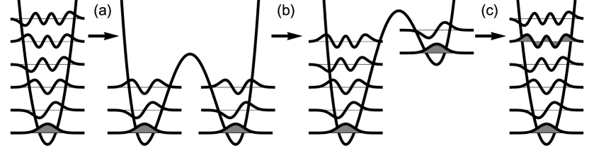
Figure 4: Scheme to prepare superpositions of the ground state and a Fock state of the harmonic oscillator, $({\ket{0}+e^{i\varphi}\ket{n}})/{\sqrt{2}}$. (a) Splitting of the ground state; (b) Biasing; (c) Merging the two wells into a harmonic trap. The shaded wave functions are the ideal initial and target states.

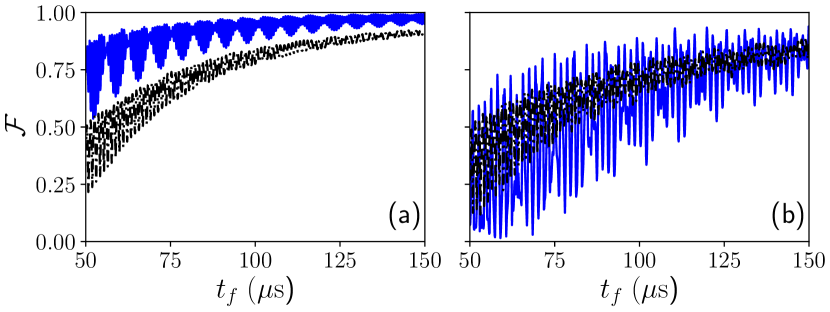
Figure 5: Comparison of the fidelities obtained after performing the multiplexing process using FAQUAD (solid blue lines) and LA method for: (a) $n=4$ and (b) $n=50$. Same parameters as in Fig. 2

The protocols studied so far are for a pure Fock state preparation. However, they also allow us to prepare states $|\psi_{\varphi}\rangle=\left(|0\rangle+e^{i\varphi}|n\rangle\right)/\sqrt{2}$ up to a relative phase $\varphi$.

A modification of the sequence in Fig. 1 leads to superposition states, see Fig. 4. The success of the protocol (step (c)) is measured with the fidelity $\mathcal{F}_{n}$ to reach $\ket{n}$ starting in the $n$th excited state of the double well, and the fidelity $\mathcal{F}_{0}(n)$ to reach $\ket{0}$ starting in the ground state while using the deformation devised to reach $\ket{n}$. (The average $(\mathcal{F}_{0}(n)+\mathcal{F}_{n})/2$ is the maximal fidelity with respect to the states labeled by $\varphi$). The upper row of Fig. 2 pictures $\mathcal{F}_{n}$ for $n=4,20,50,100$ and the lower panels the corresponding $\mathcal{F}_{0}(n)$. The $\mathcal{F}_{0}(n)$ are remarkably close to the $\mathcal{F}_{n}$, which makes superpositions $|\psi_{\varphi}\rangle$ feasible with high fidelity.

In McCormick et al. (2019) these superpositions were created via Rabi pulses for measuring deviations from a nominal trap frequency. The maximum sensitivity was reached for the superposition of the ground and the 12th state.

Discussion. We have proposed to prepare highly excited Fock states and superpositions with the ground state in trapped ions using deformations between double and single wells. Since no Rabi pulses are involved, these protocols can be applied to different atomic species or particles.

A FAQUAD approach which distributes diabatic transitions homogeneously through all the process provides a significant speedup with respect to a linear ramp of the control parameter. Methods similar in spirit to FAQUAD may also be applied Guéry-Odelin et al. (2019). The Local Adiabatic (LA) method Roland and Cerf (2002) only uses the instantaneous energy gap between the eigenstates to modulate the rate of change of the control parameter. Adapted to our multilevel scenario, we set $c_{LA}=\hbar\dot{\lambda}_{LA}\sum_{m\neq n}{[E_{n}(\lambda)-E_{m}(\lambda)]^{-2}},$ as a constant given by the boundary conditions, and parameterize $\beta(\alpha)$ as before. We have compared the performance of FAQUAD against the LA method in Fig. 5. For small $n$ FAQUAD clearly outperforms the LA, but LA is more stable as $n$ increases, due to a lesser role of quantum interferences Martínez-Garaot et al. (2015).

This paper demonstrates the potential of trap deformations to control motional states. Future work could be to find protocols for ion chains, and to make full use of the dimensionality of the parameter space Rezakhani et al. (2009), reduced here to one for simplicity. The trap deformation in our model passes through a quartic potential well with close levels that plays the role of the bottleneck of the process speed. The search for smooth, doable functional forms for the time dependence of the trap increasing the minimal gap, combined with numerical optimization of the deformation is a worthwhile objective.

References

- Martínez-Garaot et al. (2013) S. Martínez-Garaot, E. Torrontegui, X. Chen, M. Modugno, D. Guéry-Odelin, S.-Y. Tseng, and J. G. Muga, Physical Review Letters 111, 213001 (2013).
- Galland et al. (2014) C. Galland, N. Sangouard, N. Piro, N. Gisin, and T. J. Kippenberg, Physical Review Letters 112, 143602 (2014).
- Zhang et al. (2018) J. Zhang, M. Um, D. Lv, J.-N. Zhang, L.-M. Duan, and K. Kim, Phys. Rev. Lett. 121, 160502 (2018).
- Giovannetti et al. (2011) V. Giovannetti, S. Lloyd, and L. Maccone, Nature photonics 5, 222 (2011).
- Margolus and Levitin (1998) N. Margolus and L. B. Levitin, Physica D: Nonlinear Phenomena 120, 188 (1998).
- Caves and Shaji (2010) C. M. Caves and A. Shaji, Optics Communications 283, 695 (2010).
- McCormick et al. (2019) K. C. McCormick, J. Keller, S. C. Burd, D. J. Wineland, A. C. Wilson, and D. Leibfried, Nature 572, 86 (2019).
- Cirac et al. (1993) J. I. Cirac, R. Blatt, A. S. Parkins, and P. Zoller, Physical Review Letters 70, 762 (1993).
- Cirac et al. (1994) J. I. Cirac, R. Blatt, and P. Zoller, Physical Review A 49, R3174 (1994).
- Meekhof et al. (1996) D. M. Meekhof, C. Monroe, B. E. King, W. M. Itano, and D. J. Wineland, Physical Review Letters 76, 1796 (1996).
- Davidovich et al. (1996) L. Davidovich, M. Orszag, and N. Zagury, Physical Review A 54, 5118 (1996).
- de Matos Filho and Vogel (1996) R. L. de Matos Filho and W. Vogel, Phys. Rev. Lett. 76, 4520 (1996).
- Abah et al. (2019) O. Abah, R. Puebla, and M. Paternostro, (2019), arXiv:1912.05264 [quant-ph] .
- Linington et al. (2008) I. E. Linington, P. A. Ivanov, N. V. Vitanov, and M. B. Plenio, Physical Review A 77, 063837 (2008).
- Kaufmann et al. (2014) H. Kaufmann, T. Ruster, C. T. Schmiegelow, F. Schmidt-Kaler, and U. G. Poschinger, New Journal of Physics 16, 073012 (2014).
- Home and Steane (2006) J. P. Home and A. M. Steane, Quantum Information and Computation 6, 289 (2006).
- Nizamani and Hensinger (2012) A. H. Nizamani and W. K. Hensinger, Applied Physics B 106, 327 (2012).
- Fürst et al. (2014) H. A. Fürst, M. H. Goerz, U. G. Poschinger, M. Murphy, S. Montangero, T. Calarco, F. Schmidt-Kaler, K. Singer, and C. P. Koch, New Journal of Physics 16, 075007 (2014).
- Guan et al. (2011) W. Guan, S. Joseph, J. H. Park, P. S. Krstić, and M. A. Reed, Proceedings of the National Academy of Sciences 108, 9326 (2011).
- Segal and Shapiro (2006) D. Segal and M. Shapiro, Nano Letters 6, 1622 (2006).
- Torrontegui et al. (2013) E. Torrontegui, S. Ibáñez, S. Martínez-Garaot, M. Modugno, A. del Campo, D. Guéry-Odelin, A. Ruschhaupt, X. Chen, and J. G. Muga, in Advances in Atomic, Molecular, and Optical Physics, Advances In Atomic, Molecular, and Optical Physics, Vol. 62, edited by P. R. B. Ennio Arimondo and C. C. Lin (Academic Press, 2013) pp. 117 – 169.
- Guéry-Odelin et al. (2019) D. Guéry-Odelin, A. Ruschhaupt, A. Kiely, E. Torrontegui, S. Martínez-Garaot, and J. Muga, Reviews of Modern Physics 91 (2019).
- Martínez-Garaot et al. (2015) S. Martínez-Garaot, M. Palmero, D. Guéry-Odelin, and J. G. Muga, Physical Review A 92, 053406 (2015).
- Martínez-Garaot et al. (2015) S. Martínez-Garaot, A. Ruschhaupt, J. Gillet, T. Busch, and J. G. Muga, Physical Review A 92, 043406 (2015).
- Palmero et al. (2019) M. Palmero, M. Á. Simón, and D. Poletti, Entropy 21, 1207 (2019).
- Chen et al. (2011) X. Chen, E. Torrontegui, and J. G. Muga, Phys. Rev. A 83, 062116 (2011).
- Masuda and Nakamura (2010) S. Masuda and K. Nakamura, Proceedings of the Royal Society of London A: Mathematical, Physical and Engineering Sciences 466, 1135 (2010).
- Torrontegui et al. (2012) E. Torrontegui, S. Martínez-Garaot, A. Ruschhaupt, and J. G. Muga, Physical Review A 86, 013601 (2012).
- Martínez-Garaot et al. (2016) S. Martínez-Garaot, M. Palmero, J. G. Muga, and D. Guéry-Odelin, Physical Review A 94, 063418 (2016).
- Schiff (1968) L. I. Schiff, Quantum mechanics (McGraw-Hill, 1968).
- Vranivcar and Robnik (2000) M. Vranivcar and M. Robnik, Progress of Theoretical Physics Supplement 139, 214 (2000).
- Roland and Cerf (2002) J. Roland and N. J. Cerf, Physical Review A 65, 042308 (2002).
- Rezakhani et al. (2009) A. T. Rezakhani, W.-J. Kuo, A. Hamma, D. A. Lidar, and P. Zanardi, Phys. Rev. Lett. 103, 080502 (2009).