On the Injection of Relativistic Electrons in the Jet of 3C 279

Abstract

The acceleration of electrons in 3C 279 is investigated through analyzing the injected electron energy distribution (EED) in a time-dependent synchrotron self-Compton + external Compton emission model. In this model, it is assumed that relativistic electrons are continuously injected into the emission region, and the injected EED [$Q_{e}^{\prime}(\gamma^{\prime})$] follows a single power-law form with low- and high-energy cutoffs $\rm\gamma_{min}^{\prime}$ and $\rm\gamma_{max}^{\prime}$, respectively, and the spectral index $n$, i.e, $Q_{e}^{\prime}(\gamma^{\prime})\propto\gamma^{\prime-n}$. This model is applied to 14 quasi-simultaneous spectral energy distributions (SEDs) of 3C 279. The Markov Chain Monte Carlo fitting technique is performed to obtain the best-fitting parameters and the uncertainties on the parameters. The results show that the injected EED is well constrained in each state. The value of $n$ is in the range of 2.5 to 3.8, which is larger than that expected by the classic non-relativistic shock acceleration. However, the large value of $n$ can be explained by the relativistic oblique shock acceleration. The flaring activity seems to be related to an increased acceleration efficiency, reflected in an increased $\gamma^{\prime}_{\rm min}$ and electron injection power.

1 Introduction

Blazars are a subclass of active galactic nuclei (AGNs), with their relativistic jets pointing very close to our line of sight (Urry & Padovani, 1995; Ulrich et al., 1997). The non-thermal radiation produced in the relativistic jet covers from radio up to $\gamma$-ray bands. The jet emission is highly variable, with variability timescales from years to several minutes. Blazar’s spectral energy distribution (SED) presents two humps. The low-energy hump which is believed to be produced by synchrotron radiation of relativistic electrons, peaks between infrared and X-ray bands. The high-energy bump which could be produced by inverse-Compton (IC) scattering of the relativistic electrons, peaks at gamma-ray energies.

Blazars are divided into flat spectrum radio quasars (FSRQs) and BL Lacertae objects (BL Lacs) based on the rest-frame equivalent width (EW) of their broad optical emission lines (Stocke et al., 1991; Stickel et al., 1991). FSRQs have strong broad emission lines with $\rm EW>5$Å, while BL Lacs have weak or no emission lines. The synchrotron peak frequencies of FSRQ are usually $<10^{14}$ Hz, due to the strong cooling of relativistic electrons in intense external photon fields (Ghisellini & Tavecchio, 2008).

$\gamma$-rays from FSRQs could be ascribed to IC scattering of the relativistic electrons. The seed photons could be from $\sim$sub-parsec (pc) size broad-line-region (BLR) (e.g., Sikora et al., 1994; Zhang et al., 2012; Böttcher et al., 2013; Hu et al., 2015) and/or $\sim$pc-scale size dust torus (DT) (e.g., Blazejowski et al., 2000; Dermer et al., 2014; Hu et al., 2017b; Wu et al., 2018), depending on the location of the $\gamma$-ray emitting region (e.g., Ghisellini et al., 2010).

The particle acceleration mechanism in blazar jets is still a hot question. By means of numerical simulations, particle accelerations in blazar jets were explored (e.g., Sironi & Spitkovsky, 2009; Sironi et al., 2015; Summerlin & Baring, 2012; Guo et al., 2015). The studies of numerical simulation focus on micro-physics and acceleration efficiency. However, there is a gap between the numerical simulations and the observations.

Diffusive shock acceleration is the mostly discussed particle acceleration mechanism. The power-law form of particle distribution is a key feature of this mechanism. For non-relativistic shock acceleration, the index of the particle distribution only depends on the shock compression ratio $r$, i.e, the power-law index $n=(r+2)/(r-1)$ (e.g., Drury et al., 1983; Jones & Ellison, 1991). For strong shock with $r=4$, the canonical $n\simeq 2$ is obtained (e.g., Drury et al., 1983; Jones & Ellison, 1991). For the accelerations at relativistic shocks, a wide variety of power-law indices is feasible, depending on the properties of the shock and the magnetic field (Kirk & Heavens, 1989; Ellison et al, 1990; Ellison & Double, 2004; Summerlin & Baring, 2012; Baring et al, 2017).

By fitting observed data with a proper emission model, one can obtain emitting EED. It is the result of the competition between acceleration/injection and cooling, and it can be used to investigate the acceleration mechanism (e.g., Massaro et al., 2006; Yan et al., 2013; Zhou et al, 2014). However, this tactic is only suitable for the blazars in which the cooling effect does not significantly re-shape the accelerated/injected electron distribution, like Mrk 421 and Mrk 501 (Ushio et al., 2010; Tramacere et al., 2011; Yan et al., 2013; Peng et al., 2014) (i.e., the high-synchrotron-peaked BL Lacs).

In FSRQs, the strong radiative cooling of electrons due to the IC scattering off external photons has a big impact on the evolution of the emitting EED. Hence, the emitting EED cannot be directly connected to acceleration process.

Here, we investigate the acceleration process of the electrons in the FSRQ 3C 279 through analyzing the injected EEDs in a time-dependent radiative model. Throughout the paper, we adopt the cosmological parameters $\rm H_{0}=69.6~{}km~{}s^{-1}~{}Mpc^{-1}$, $\Omega_{M}=0.286$, and $\Omega_{\Lambda}=0.714$. This results in the luminosity distance $d_{L}=3113.6~{}\rm Mpc$ for 3C 279 with redshift $z=0.536$.

2 Method

We adopt a one-zone homogeneous leptonic jet model. It is assumed that emissions are produced in a spherical blob of radius $R^{\prime}$ filled with a uniform magnetic field $B^{\prime}$. The blob moves with a relativistic speed $\beta_{\Gamma}c=c(1-1/\Gamma^{2})^{1/2}$ and an angle $\theta$ with respect to the line of sight, where $c$ is the speed of light and $\Gamma$ is the bulk Lorentz factor of the blob. The observed radiations are strongly boosted by the relativistic Doppler factor $\delta_{D}=1/[\Gamma(1-\beta_{\Gamma}\cos\theta)]$. It is assumed $\theta\sim 1/\Gamma$, resulting in $\delta_{D}\sim\Gamma$. Here and throughout this paper, primed quantities refer to the frame comoving with the blob and unprimed quantities refer to the observer’s frame.

2.1 Solving emitting EED

In the model, we assume that the accelerated electrons are continuously injected into the blob. The isotropic electrons loss energy through synchrotron radiation and IC scattering, and may also escape out of the blob. The evolution of the electrons in the comoving frame of the blob is governed by (e.g., Coppi et al, 1990; Chiaberge & Ghisellini, 1999)

$$\frac{\partial{N_{e}^{\prime}(\gamma^{\prime})}}{\partial{t}}+\frac{\partial}{\partial{\gamma^{\prime}}}\left[\dot{\gamma}^{\prime}N_{e}^{\prime}(\gamma^{\prime})\right]+\frac{N_{e}^{\prime}(\gamma^{\prime})}{t^{\prime}_{\rm esc}}=\dot{Q}_{e}^{\prime}\ ,$$ (1)

where $N_{e}^{\prime}(\gamma^{\prime})$ is the number of the electrons per unit $\gamma^{\prime}$, $\dot{\gamma}^{\prime}$ is the total energy-loss rate of the electrons, $t^{\prime}_{\rm esc}$ is the escape timescale of the electrons, and $\dot{Q}_{e}$ is the source term describing the injection rate of the electrons in units of $s^{-1}$.

The injected EED is assumed to be a single power-law distribution,

$$Q_{e}^{\prime}(\gamma^{\prime})=Q_{0}^{\prime}\gamma^{\prime-n},~{}\gamma_{\rm min}^{\prime}\leq\gamma^{\prime}\leq\gamma_{\rm max}^{\prime},$$ (2)

with

$$Q_{0}^{\prime}=\left\{\begin{tabular}[]{l}$\frac{P^{\prime}_{e}}{m_{e}c^{2}}\frac{2-n}{{\gamma_{\rm max}^{\prime}}^{2-n}-{\gamma_{\rm min}^{\prime}}^{2-n}};~{}n\neq 2$\\ $\frac{P^{\prime}_{e}}{m_{e}c^{2}\ln\left(\gamma_{\rm max}^{\prime}/\gamma_{\rm min}^{\prime}\right)};~{}n=2$\\ \end{tabular}\right.,$$ (3)

where $\gamma_{\rm min}^{\prime}$ and $\gamma_{\rm max}^{\prime}$ are respectively the low and high energy cutoffs, and $P^{\prime}_{e}$ is the injection power in the units of $\rm erg/s$, and $n$ is the spectral index (Böttcher & Chiang, 2002).

Three radiative energy losses of the electrons are considered:

(1) synchrotron radiation cooling

$$-\dot{\gamma}^{\prime}_{\rm syn}=\frac{4\sigma_{T}}{3m_{e}c}{U_{B}^{\prime}\gamma^{\prime}}^{2},$$ (4)

where $U_{B}^{\prime}={B^{\prime}}^{2}/8\pi$ is the magnetic field energy density.

(2) synchrotron self-Compton radiation (SSC) cooling (e.g., Jones, 1968; Blumenthal & Gould, 1970; Finke et al., 2008)

$$-\dot{\gamma}^{\prime}_{\rm ssc}=\frac{4\sigma_{T}}{3m_{e}c}{\gamma^{\prime}}^{2}\int_{0}^{\infty}d\epsilon^{\prime}u_{syn}^{\prime}(\epsilon^{\prime})f_{kn}(\epsilon^{\prime},\gamma^{\prime}),$$ (5)

where $u_{\rm syn}^{\prime}(\epsilon^{\prime})\simeq(\sigma_{\rm T}U_{B}^{\prime})/(2\pi R^{\prime 2}\epsilon^{\prime})\gamma_{s}^{\prime 3}N^{\prime}_{e}(\gamma_{s}^{\prime})$ is the spectral energy density of the synchrotron radiation. Here, $\gamma_{s}^{\prime}=\sqrt{\epsilon^{\prime}B_{\rm cr}/B^{\prime}}$ is a synchrotron-emitting electron’s Lorentz factor where $B_{\rm cr}\simeq 4.414\times 10^{13}$ G is the critical magnetic field.

$$f_{kn}(\epsilon^{\prime},\gamma^{\prime})=\frac{9}{16}\int_{\gamma^{\prime}_{\rm low}}^{\gamma^{\prime}}d\gamma^{\prime\prime}F_{c}(x,q)\frac{\gamma^{\prime}-\gamma^{\prime\prime}}{{\epsilon^{\prime}}^{2}{\gamma^{\prime}}^{4}},$$ (6)

where the lower limit for the integration is $\gamma^{\prime}_{\rm low}\simeq\gamma^{\prime}+\epsilon^{\prime}-\frac{4{\gamma^{\prime}}^{2}\epsilon^{\prime}}{1+4\gamma^{\prime}\epsilon^{\prime}}$, and

$$F_{c}(x,q)=\Big{[}2q\ln{q}+q+1-2q^{2}+\frac{(xq)^{2}}{2(1+xq)}(1-q)\Big{]}\ .$$ (7)

Here, $x=4\epsilon^{\prime}\gamma^{\prime}$, $q=\frac{\epsilon_{\gamma}^{\prime}/\gamma^{\prime}}{x(1-\epsilon_{\gamma}^{\prime}/\gamma^{\prime})}$, and $\epsilon_{\gamma}^{\prime}=\gamma^{\prime}+\epsilon^{\prime}-\gamma^{\prime\prime}$ is the scattered photon energy required by the conservation of energy. The limits on $q$ are $\frac{1}{4\gamma^{\prime 2}}\leq q\leq 1$.

(3) external-Compton (EC) cooling

$$-\dot{\gamma}^{\prime}_{\rm ec}=\frac{4\sigma_{T}}{3m_{e}c}\gamma^{2}\int_{0}^{\infty}d\epsilon u_{ext}(\epsilon)f_{kn}(\epsilon,\gamma)\ ,$$ (8)

where $u_{\rm ext}(\epsilon)$ is the spectral energy density of the external photon field. The quantities $\gamma=\delta_{D}\gamma^{\prime}$ and $\epsilon$ refer to the stationary frame with respect to the black hole (BH).

For the EC processes, we consider the seed photons from BLR and DT. In this work, BLR and IR DT radiations are assumed to be a dilute blackbody (e.g., Liu & Bai, 2006; Tavecchio & Ghisellini, 2008),

$$u_{ext}(\epsilon)=\frac{15U_{0}}{(\pi\Theta)^{4}}\frac{\epsilon^{3}}{\exp\left(\epsilon/\Theta\right)-1}\ ,$$ (9)

where $\Theta$ and $U_{0}$ are the dimensionless temperature and energy density of the BLR/DT radiation field, respectively. We consider the BLR radiation with $\Theta\simeq 9.6\times 10^{4}$ K/($5.93\times 10^{9}$ K) (corresponding to $\sim 2\times 10^{15}$ Hz) and $\rm U_{0}\simeq 2.7\times 10^{-2}\ erg\ cm^{-3}$ (e.g., Ghisellini & Tavecchio, 2008), and the IR DT radiation with $\Theta\simeq 1.4\times 10^{3}$ K/($5.93\times 10^{9}$ K) (corresponding to $\sim 3\times 10^{13}$ Hz) and $\rm U_{0}\simeq 2.1\times 10^{-4}\ erg\ cm^{-3}$ (e.g., Ghisellini & Tavecchio, 2009).

Therefore, the total cooling rate of the electrons is $\dot{\gamma}^{\prime}=\dot{\gamma}^{\prime}_{\rm syn}+\dot{\gamma}^{\prime}_{\rm ssc}+\dot{\gamma}^{\prime}_{\rm ec}$. We simply assume an energy-independent escape for the electrons, i.e., $t^{\prime}_{\rm esc}=\eta_{\rm esc}R^{\prime}/c$, where it is required that $\eta>1$ (e.g., Böttcher & Chiang, 2002). With the above information, Equation (1) is solved by using the iterative scheme described by Graff et al. (2008) to obtain the steady-state EED.

2.2 Calculation of emission spectra

The spectra of synchrotron radiation, SSC and EC are calculated with the formulas in Finke et al. (2008); Dermer et al. (2009). We here give the key formulas. The synchrotron spectrum is

$$\nu f_{\nu}^{\rm syn}=\frac{\delta_{D}^{4}\sqrt{3}e^{3}B^{\prime}}{4\pi hd_{L}^{2}}\chi(\tau)\epsilon^{\prime}\int_{1}^{\infty}d\gamma^{\prime}N_{e}^{\prime}(\gamma^{\prime})R_{s}(\epsilon^{\prime}/\epsilon^{\prime}_{c}),$$ (10)

where $\epsilon^{\prime}m_{e}c^{2}=(1+z)h\nu/\delta_{D}$, $e$ is the fundamental charge and $h$ is the Planck constant. In the spherical approximation, the factor $\chi(\tau)\equiv 3u(\tau)/\tau$, where $\tau=2\kappa_{\epsilon^{\prime}}R^{\prime}$ is the synchrotron self-absorption (SSA) opacity and $u(\tau)=\frac{1}{2}\Big{(}1-\frac{2}{\tau^{2}}[1-(1+\tau)\exp(-\tau)]\Big{)}$. The SSA coefficient is given by

$$\kappa_{\epsilon^{\prime}}=-\frac{\sqrt{3}B^{\prime}e^{3}\lambda_{c}^{3}}{8\pi hm_{e}c^{3}{\epsilon^{\prime}}^{2}}\int_{1}^{\infty}d\gamma^{\prime}R_{s}(\frac{\epsilon^{\prime}}{\epsilon^{\prime}_{c}})\Big{[}{\gamma^{\prime}}^{2}\frac{\partial}{\partial\gamma^{\prime}}\Big{(}\frac{N_{e}^{\prime}(\gamma^{\prime})}{{\gamma^{\prime}}^{2}}\Big{)}\Big{]}\ ,$$ (11)

where $m_{e}$ is the rest mass of electron and $\lambda_{c}=h/m_{e}c=2.43\times 10^{-10}~{}\rm cm$ is the electron Compton wavelength. Here, $\epsilon_{c}^{\prime}=\frac{3eB^{\prime}h}{4\pi m_{e}^{2}c^{3}}{\gamma^{\prime}}^{2}$ is the characteristic energy of synchrotron radiation in the units of $m_{e}c^{2}$, and $R_{s}(x)=(x/2)\int_{0}^{\pi}{d\theta}\sin\theta\int_{x/\sin\theta}^{\infty}{dtK_{5/3}(t)}$.

The SSC/EC spectrum is given by

$$\nu f_{\nu}^{\rm SSC/EC}=f_{L}\epsilon_{\gamma}^{\prime 2}\int_{0}^{\infty}{}d\epsilon^{\prime}\frac{u_{\rm syn/ext}^{\prime}(\epsilon^{\prime})}{\epsilon^{\prime 2}}\int_{1}^{\infty}{}d\gamma^{\prime}{}\frac{N_{e}^{\prime}(\gamma^{\prime})}{\gamma^{\prime 2}}F_{c}(x,q),$$ (12)

where $\epsilon_{\gamma}^{\prime}m_{e}c^{2}=(1+z)h\nu/\delta_{D}$, $f_{L}=(3c\sigma_{T}\delta_{D}^{4})/(16\pi d_{L}^{2})$, and $u_{\rm ext}^{\prime}(\epsilon^{\prime})=\delta_{\rm D}^{3}u_{\rm ext}(\epsilon^{\prime}/\delta_{\rm D})$ (e.g., Dermer et al., 2009; Ghisellini & Tavecchio, 2009).

The model is characterized by eight parameters, i.e., $B^{\prime},\delta_{D},P^{\prime}_{e},n,\gamma_{\rm min}^{\prime},\gamma_{\rm max}^{\prime},\eta_{\rm esc}$ and $R^{\prime}$. The radius of the emission region can be estimated from the minimum variability timescale $t_{\rm var}$, i.e., $R^{\prime}=c\delta_{D}t_{\rm var}/(1+z)$.

2.3 MCMC fitting technique

In order to unbiasedly constrain the model parameters, we adopt MCMC technique which is based on Bayesian statistics to perform fitting. The MCMC fitting technique is a powerful tool to explore the multi-dimensional parameter space in blazar science (Yan et al., 2013, 2015). The details on MCMC technique can be found in Lewis & Bridle (2002); Yuan et al. (2011); Liu et al. (2012).

3 Application to 3C 279

3C 279 is one of the best studied FSRQs. It has been intensively monitored from radio band to $\gamma$-ray energies (e.g., Wehrle et al., 1998; Hartman et al., 1996; Böttcher et al., 2007; Collmar et al., 2010; Abdo et al., 2010; Hayashida et al., 2012, 2015; Pacciani et al., 2014; Aleksic et al., 2015). 3C 279 shows rapid variabilities at all wavelengths. The radio and optical emissions are highly-polarized. The correlations between the optical polarization level/angle and $\gamma$-ray variabilities provide strong evidence for the SSC+EC model (e.g., Abdo et al., 2010; Paliya et al., 2015; Hayashida et al., 2012).

Hayashida et al. (2012, 2015) and Paliya et al. (2015) have constructed 16 high-quality SEDs for 3C 279 from (quasi-)simultaneous observations by Fermi satellite together with many other facilities. Note that there is a temporal overlap of Period H in Hayashida et al. (2012) with the low-activity state in Paliya et al. (2015), and the X-ray data are lacking in period B in Hayashida et al. (2015). We therefore do not consider the SED in the low-activity state in Paliya et al. (2015) and the one in period B in Hayashida et al. (2015). We apply the method described in Section 2 to the rest of 14 high-quality SEDs. In our fitting, the radio data of $\lesssim 200\$GHz are neglected, due to the fact that the low-frequency radio emission comes from the large-scale jet.

Paliya et al. (2015) showed that the $\gamma$-ray variability timescale $t_{\rm var}$ can be down to $\sim 1-2$ hours, and Hayashida et al. (2015) reported $t_{\rm var}\sim 2$ hours in the flare state of Period D. In addition, variabilities down to the timescale of a few hours were also reported in Hayashida et al. (2012). Hence, to reduce the number of model parameters, we take $\rm t_{\rm var}$ = 2 hours in the fittings. In the process of testing our method, it is found that the observed data is insensitive to $\gamma^{\prime}_{\rm max}$. We then fix it to a large value, $\gamma^{\prime}_{\rm max}=3\times 10^{4}$. There are finally six free parameters in the fittings.

Following Poole et al. (2008) and Abdo et al. (2011), a relative systematic uncertainty, namely 5% of the data, is added in quadrature to the statistical error of the IR-optical-UV and X-rays data. This is due to the fact that the errors of these data are dominated by the systematic errors.

Table 1: Mean values and marginalized 95% CI of the parameters for the SED fittings with the DT photons.

	$B^{\prime}$ (G)	$\delta_{\rm D}$ (10)	$\eta_{\rm esc}$ (10)	$P_{e}^{\prime}\ (10^{41}\ \rm erg/s)$	$\gamma_{\rm min}^{\prime}\ (10^{2})$	$n$	$\chi_{\rm DT}^{2}\ (dof)$
$\rm Period~{}A$	$1.02\pm 0.02$	$3.78\pm 0.08$	$7.67$	$4.27\pm 0.19$	$2.48\pm 0.21$	$2.82\pm 0.04$	0.69(34)
95% CI	0.97 - 1.08	3.64 - 3.94	$\geq 2.72$	3.97 - 4.71	2.04 - 2.86	2.74 - 2.90
$\rm Period~{}B$	$0.67\pm 0.06$	$4.10\pm 0.14$	$2.30$	$10.21\pm 1.46$	$2.89\pm 0.44$	$2.49\pm 0.10$	1.47(17)
95% CI	0.56 - 0.80	3.84 - 4.41	$\geq 0.18$	7.73 - 13.99	1.95 - 3.80	2.31 - 2.70
$\rm Period~{}C$	$1.40\pm 0.07$	$4.68\pm 0.13$	$2.78\pm 0.77$	$4.62\pm 0.27$	$2.66\pm 0.20$	$3.16\pm 0.06$	3.10(36)
95% CI	1.27 - 1.52	4.45 - 4.93	1.24 - 4.26	4.13 - 5.16	2.26 - 3.04	3.03 - 3.28
$\rm Period~{}D$	$1.19\pm 0.05$	$4.75\pm 0.15$	$4.75$	$5.17\pm 0.56$	$4.66\pm 0.40$	$3.62\pm 0.09$	1.97(16)
95% CI	1.09 - 1.29	4.48 - 5.07	$\geq 0.83$	4.14 - 6.30	3.93 - 5.55	3.45 - 3.80
$\rm Period~{}E$	$1.46\pm 0.19$	$3.91\pm 0.15$	$5.90$	$3.74\pm 0.38$	$3.83\pm 0.23$	$3.44\pm 0.04$	2.82(21)
95% CI	1.23 - 2.03	3.50 - 4.15	$\geq 1.31$	3.04 - 4.56	3.34 - 4.28	3.35 - 3.53
$\rm Period~{}F$	$1.44\pm 0.17$	$3.46\pm 0.24$	$5.73$	$5.31\pm 0.65$	$3.73\pm 0.51$	$3.49\pm 0.24$	0.26(12)
95% CI	1.14 - 1.80	3.01 - 3.95	$\geq 1.08$	4.26 - 6.86	2.89 - 4.85	3.01 - 3.95
$\rm Period~{}G$	$0.97\pm 0.11$	$3.81\pm 0.29$	$5.82$	$9.13\pm 1.86$	$6.33\pm 1.44$	$3.31\pm 0.11$	0.66(13)
95% CI	0.76 - 1.21	3.29 - 4.41	$\geq 1.32$	6.25 - 13.73	4.03 - 9.42	3.10 - 3.52
$\rm Period~{}H$	$0.86\pm 0.15$	$3.57\pm 0.28$	$5.29$	$5.21\pm 0.78$	$2.84\pm 0.33$	$3.53\pm 0.24$	0.45(16)
95% CI	0.61 - 1.20	3.08 - 4.18	$\geq 0.98$	3.94 - 6.94	2.21 - 3.49	3.07 - 4.00
$\rm Flare1$	$1.06\pm 0.08$	$3.72\pm 0.15$	$5.91$	$10.15\pm 1.59$	$8.77\pm 1.41$	$3.35\pm 0.09$	1.88(19)
95% CI	0.91 - 1.23	3.44 - 4.02	$\geq 1.72$	7.51 - 13.75	6.34 - 11.88	3.19 - 3.55
$\rm Flare2{\dagger}$	$0.87\pm 0.04$	$4.39\pm 0.09$	$1.05\pm 0.54$	$1.28\pm 0.10$	$6.48\pm 0.61$	$3.26\pm 0.05$	2.00(20)
95% CI	0.79 - 0.95	4.23 - 4.57	0.43 - 2.53	1.10 - 1.49	5.35 - 7.80	3.17 - 3.36
$\rm Post-flare$	$2.00\pm 0.32$	$4.67\pm 0.58$	$5.07$	$4.07\pm 1.10$	$3.31\pm 1.48$	$3.25\pm 0.05$	0.92(18)
95% CI	1.39 - 2.64	3.59 - 5.82	$\geq 0.58$	2.56 - 7.12	1.48 - 7.42	3.14 - 3.36
$\rm Period~{}A15$	$1.52\pm 0.12$	$4.33\pm 0.22$	$20.01$	$4.14\pm 0.41$	$2.76\pm 0.53$	$3.39\pm 0.06$	0.68(34)
95% CI	1.28 - 1.78	3.78 - 4.64	$\geq 8.97$	3.50 - 5.14	2.12 - 4.11	3.28 - 3.51
$\rm Period~{}C15$	$1.09\pm 0.06$	$3.90\pm 0.10$	$0.68\pm 0.30$	$10.96\pm 0.60$	$4.82\pm 0.43$	$3.41\pm 0.06$	1.82(30)
95% CI	0.99 - 1.22	3.71 - 4.08	0.29 - 1.42	9.86 - 12.22	4.00 - 5.71	3.28 - 3.54
$\rm Period~{}D15$	$0.52\pm 0.05$	$4.34\pm 0.18$	$0.25\pm 0.10$	$38.7\pm 7.3$	$8.30\pm 1.32$	$3.28\pm 0.05$	1.31(20)
95% CI	0.44 - 0.62	4.01 - 4.70	0.12-0.52	2.68 - 5.50	5.98 - 11.25	3.19 - 3.39

Table 2: Mean values and marginalized 95% CI of the parameters for the SED fittings with the BLR photons.

	$B^{\prime}$ (G)	$\delta_{\rm D}$ (10)	$\eta_{\rm esc}$ (10)	$P_{e}^{\prime}\ (10^{42}\rm\ erg/s)$	$\gamma_{\rm min}^{\prime}\ (10^{2})$	$n$	$\chi_{\rm BLR}^{2}\ (dof)$
$\rm Period~{}A$	$5.57\pm 0.15$	$2.04\pm 0.02$	$5.86$	$2.50\pm 0.09$	$1.64\pm 0.08$	$3.18\pm 0.04$	2.10(34)
95% CI	5.28 - 5.88	2.00 - 2.08	$\geq 0.20$	2.36 - 2.76	1.48 - 1.80	3.10 - 3.27
$\rm Period~{}B$	$2.11\pm 0.70$	$2.25\pm 0.12$	$4.71$	$6.55\pm 1.78$	$1.92\pm 0.38$	$2.69\pm 0.26$	1.95(17)
95% CI	1.36 - 3.83	2.10 - 2.52	$\geq 0.16$	3.53 - 9.57	1.02 - 2.50	2.32 - 3.26
$\rm Period~{}C$	$7.06\pm 0.32$	$2.46\pm 0.02$	$5.62$	$2.58\pm 0.08$	$2.19\pm 0.09$	$3.62\pm 0.06$	2.71(36)
95% CI	6.41 - 7.69	2.42 - 2.51	$\geq 1.03$	2.42 - 2.75	2.02 - 2.34	3.49 - 3.74
$\rm Period~{}D$	$6.13\pm 0.32$	$2.79\pm 0.04$	$5.29$	$2.62\pm 0.12$	$2.35\pm 0.18$	$4.02\pm 0.09$	2.45(16)
95% CI	5.52 - 6.79	2.72 - 2.86	$\geq 0.50$	2.40 - 2.85	2.02 - 2.72	3.85 - 4.19
$\rm Period~{}E$	$8.54\pm 0.66$	$2.26\pm 0.06$	$5.00$	$2.01\pm 0.13$	$1.83\pm 0.09$	$3.61\pm 0.05$	2.91(21)
95% CI	7.37 - 9.84	2.14 - 2.38	$\geq 0.37$	1.76 - 2.27	1.66 - 2.01	3.52 - 3.71
$\rm Period~{}F$	$7.93\pm 0.96$	$1.77\pm 0.08$	$5.19$	$3.64\pm 0.34$	$2.54\pm 0.28$	$3.62\pm 0.22$	0.40(12)
95% CI	6.15 - 9.78	1.59 - 1.93	$\geq 0.54$	3.11 - 4.45	2.08 - 3.18	3.20 - 4.06
$\rm Period~{}G$	$5.07\pm 0.50$	$2.36\pm 0.07$	$5.13$	$3.72\pm 0.28$	$2.67\pm 0.25$	$3.56\pm 0.11$	1.18(13)
95% CI	4.16 - 6.16	2.23 - 2.50	$\geq 0.37$	3.22 - 4.31	2.23 - 3.19	3.35 - 3.77
$\rm Period~{}H$	$3.34\pm 1.23$	$1.58\pm 0.11$	$4.59$	$4.53\pm 1.42$	$1.91\pm 0.28$	$3.34\pm 0.35$	0.64(16)
95% CI	1.74 - 6.50	1.41 - 1.82	$\geq 0.12$	2.56 - 8.06	1.24 - 2.37	2.82 - 4.16
$\rm Flare1$	$6.19\pm 0.48$	$2.68\pm 0.05$	$5.21$	$3.11\pm 0.20$	$2.58\pm 0.24$	$3.58\pm 0.05$	2.28(19)
95% CI	5.33 - 7.20	2.58 - 2.79	$\geq 0.55$	2.74 - 3.54	2.13 - 3.11	3.48 - 3.68
$\rm Flare2$	$4.95\pm 0.23$	$3.14\pm 0.03$	$5.81$	$3.80\pm 0.16$	$2.24\pm 0.11$	$3.74\pm 0.04$	7.33(20)
95% CI	4.51 - 5.40	3.07 - 3.20	$\geq 1.04$	3.49 - 4.13	2.02 - 2.46	3.66 - 3.82
$\rm Post-flare$	$10.13\pm 1.46$	$2.55\pm 0.11$	$5.13$	$2.41\pm 0.20$	$1.92\pm 0.44$	$3.44\pm 0.06$	0.85(18)
95% CI	7.37 - 13.05	2.32 - 2.76	$\geq 0.40$	2.12 - 2.89	1.26 - 2.97	3.32 - 3.55
$\rm Period~{}A15$	$5.61\pm 0.38$	$2.03\pm 0.05$	$6.14$	$3.36\pm 0.12$	$3.10\pm 0.16$	$3.62\pm 0.07$	1.35(34)
95% CI	4.95 - 6.45	1.92 - 2.13	$\geq 1.46$	3.15 - 3.59	2.79 - 3.43	3.48 - 3.76
$\rm Period~{}C15$	$4.49\pm 0.28$	$2.27\pm 0.05$	$4.65$	$5.21\pm 0.22$	$3.47\pm 0.14$	$3.76\pm 0.07$	2.24(30)
95% CI	3.98 - 5.08	2.16 - 2.37	$\geq 0.11$	4.81 - 5.70	3.20 - 3.71	3.61 - 3.90
$\rm Period~{}D15$	$2.86\pm 0.22$	$3.46\pm 0.07$	$5.24$	$6.69\pm 0.51$	$2.81\pm 0.25$	$3.89\pm 0.05$	3.55(20)
95% CI	2.46 - 3.34	3.32 - 3.60	$\geq 0.54$	5.78 - 7.75	2.36 - 3.33	3.80 - 3.98

Table 3: Mean values and marginalized 95% CI of the derived parameters for the SED fittings with the DT photons.

state	$\log_{10}\gamma_{c}^{\prime}$	$\log_{10}L_{B}$ (erg/s)	$\log_{10}L_{r}$ (erg/s)
$\rm Period~{}A$	$0.82\pm 0.16$	$44.19\pm 0.04$	$44.17\pm 0.02$
95% CI	$\leq$ 1.29	44.11 $-$ 44.29	44.14 $-$ 44.20
$\rm Period~{}B$	$1.40\pm 0.39$	$43.97\pm 0.13$	$44.59\pm 0.02$
95% CI	$\leq$ 2.22	43.71 $-$ 44.25	44.54 $-$ 44.64
$\rm Period~{}C$	$0.98\pm 0.16$	$44.84\pm 0.08$	$44.38\pm 0.01$
95% CI	0.74 $-$ 1.36	44.68 $-$ 45.00	44.36 $-$ 44.40
$\rm Period~{}D$	$0.82\pm 0.32$	$44.72\pm 0.08$	$44.45\pm 0.02$
95% CI	$\leq$ 1.53	44.56 $-$ 44.90	$44.41-44.49$
$\rm Period~{}E$	$0.88\pm 0.24$	$44.56\pm 0.06$	$44.13\pm 0.06$
95% CI	$\leq$ 1.50	44.45 $-$ 44.69	$43.96-44.23$
$\rm Period~{}F$	$1.01\pm 0.27$	$44.33\pm 0.19$	$44.17\pm 0.04$
95% CI	$\leq$ 1.67	43.95 $-$ 44.69	44.10 $-$ 44.24
$\rm Period~{}G$	$0.96\pm 0.25$	$44.15\pm 0.22$	$44.51\pm 0.03$
95% CI	$\leq$ 1.51	43.71 $-$ 44.60	44.45 $-$ 44.58
$\rm Period~{}H$	$1.12\pm 0.29$	$43.94\pm 0.28$	$44.18\pm 0.04$
95% CI	$\leq$ 1.84	43.41 $-$ 44.50	44.11 $-$ 44.26
$\rm Flare1$	$0.94\pm 0.21$	$44.20\pm 0.13$	$44.54\pm 0.04$
95% CI	$\leq$ 1.44	43.94 $-$ 44.46	$44.48-44.62$
$\rm Flare2{\dagger}$	$1.54\pm 0.20$	$44.32\pm 0.07$	$44.76\pm 0.02$
95% CI	1.10 $-$ 1.88	44.18 $-$ 44.46	44.73 $-$ 44.80
$\rm Post-flare$	$0.73\pm 0.33$	$45.12\pm 0.35$	$44.30\pm 0.03$
95% CI	$\leq$ 1.57	44.36 $-$ 45.77	44.24 $-$ 44.38
$\rm Period~{}A15$	$0.21\pm 0.17$	$44.78\pm 0.16$	$44.27\pm 0.02$
95% CI	$\leq$0.62	44.42 $-$ 45.02	$44.24-44.32$
$\rm Period~{}C15$	$1.83\pm 0.16$	$44.31\pm 0.06$	$44.55\pm 0.03$
95% CI	1.50 $-$ 2.14	44.19 $-$ 44.43	44.48 $-$ 44.60
$\rm Period~{}D15$	$2.20\pm 0.18$	$43.85\pm 0.14$	$45.16\pm 0.04$
95% CI	1.81 $-$ 2.49	43.59 $-$ 44.13	45.07 $-$ 45.25

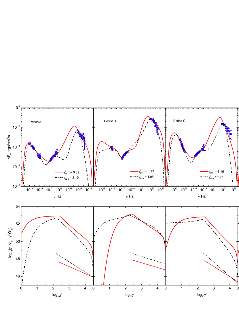
Figure 1: Upper panels: Best-fitting results for the SEDs of 3C 279 during the observations of Periods A, B, C and D reported in Hayashida et al. (2012). The red solid line and black dash-dotted line represent the fittings with the seed photons from the DT and the BLR, respectively. Lower panels: The steady-state emitting EED and injected EED corresponding to the best-fitting model in each state. The red solid thick and thin lines are respectively the steady-state emitting EED and the injected EED obtained from the fitting with the seed photons from the DT; and the black dash-dotted thick and thin lines are respectively the steady-state emitting EED and injected EED obtained from the fitting with the seed photons from the BLR.

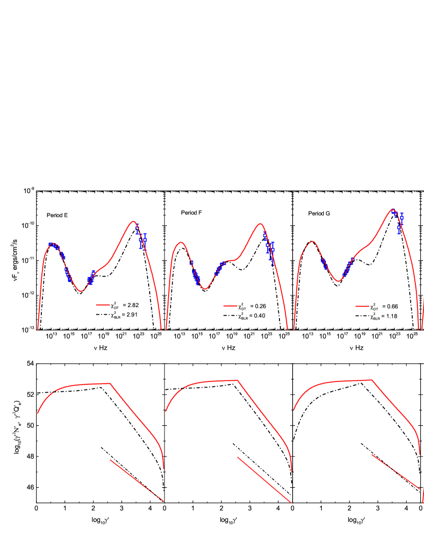
Figure 2: Same as Figure 1, but for the SEDs in Periods E, F, G, H reported by Hayashida et al. (2012).

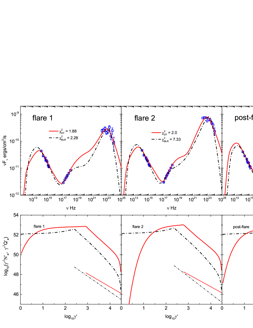
Figure 3: Same as Fig.2, but for the SEDs reported in Paliya et al.(2015).

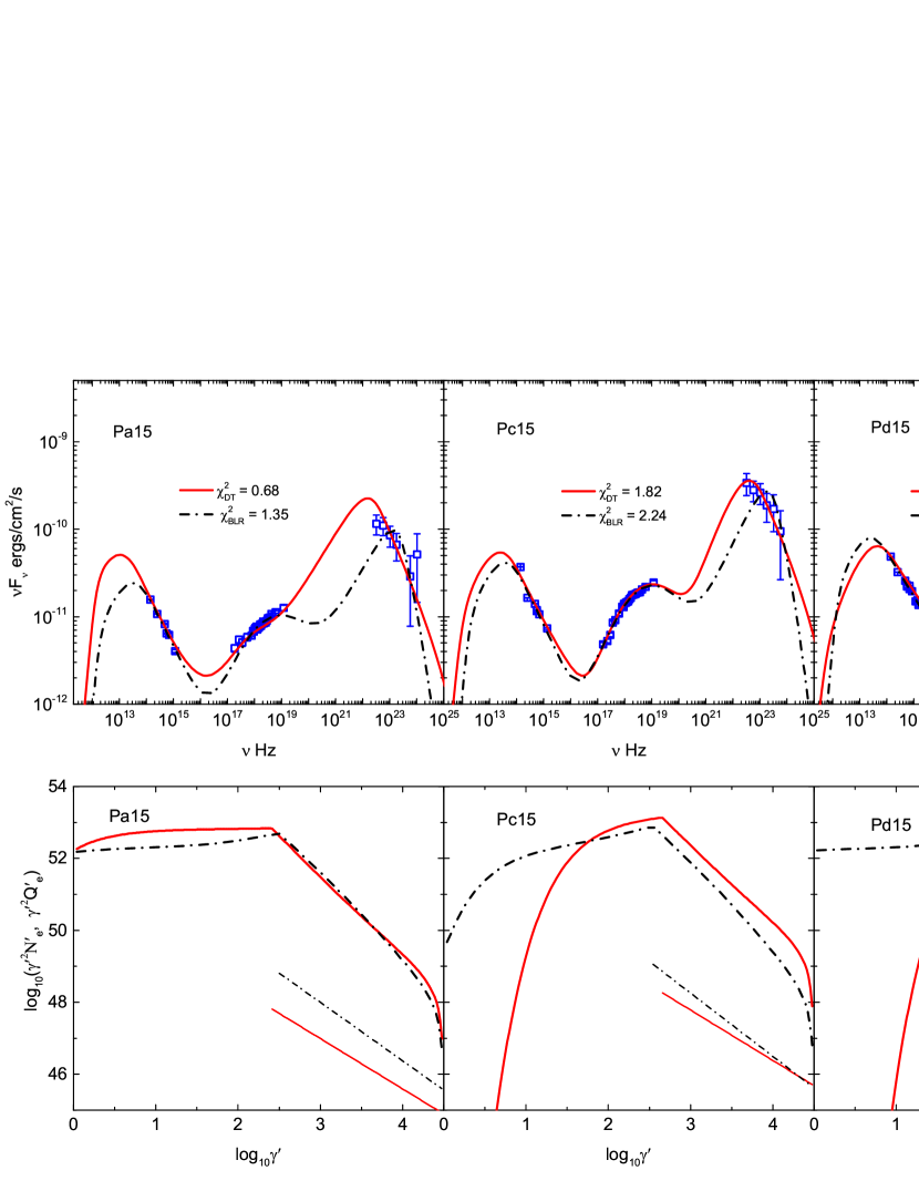
Figure 4: Same as Fig.2, but for the SEDs reported in Hayashida et al. (2015).

3.1 Fitting the SEDs

In the upper panels of Figures 1-4, we show the best-fitting results for the 14 SEDs. Each SED is fitted with two models: the model with the BLR photons and the model with the DT photons. The corresponding reduced $\rm\chi^{2}_{DT/BLR}$ is reported in each panel. One can see that all the fittings with the DT photons, except for Period C in Hayashida et al. (2012), are better than that with the BLR photons. The highest-energy X-ray/gamma-ray data can be fitted better with the model of SSC+EC-DT. In the SSC+EC-BLR model, the Klein-Nishina (KN) effect becomes important and suppresses the gamma-ray emission, leading to the mismatch between the data and the model (e.g., the first panel in Fig. 1). In addition, the high-energy hump in the SSC+EC-BLR model locates at higher energies, which causes the worse fitting to the X-ray data (e.g., the third panel in Fig. 4)

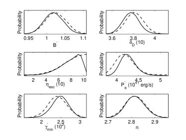
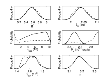
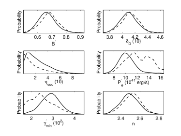
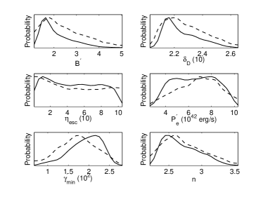
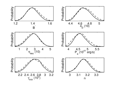
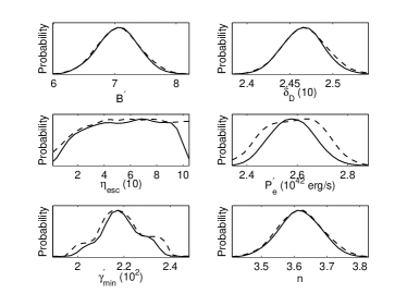
Figure 6: 1D probability distributions of the free model parameters obtained from SED fittings with the seed photons from DT (left panels) and BLR (right panels). The dashed lines show the maximum likelihood distributions and solid lines show the marginalized probability distributions. From top to bottom, the plots are the results obtained from fitting the SEDs in Periods A, B, and C reported in Hayashida et al.(2012), respectively.

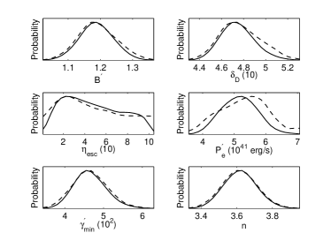
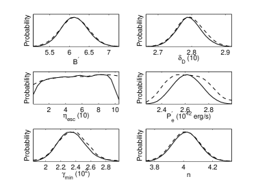
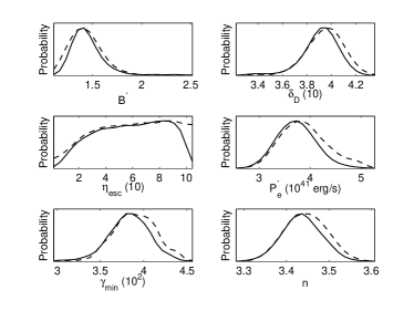
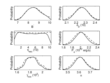
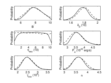
Figure 7: Same as Figure 6, but for the SEDs in Periods D (Top), E(Middle) and F(Bottom) reported in Hayashida et al.(2012).

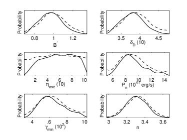
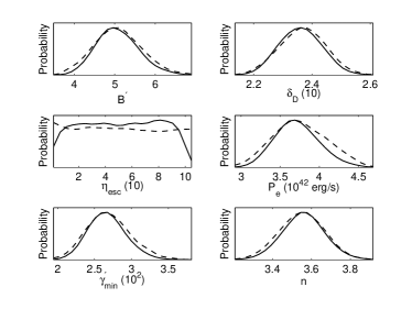
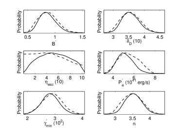
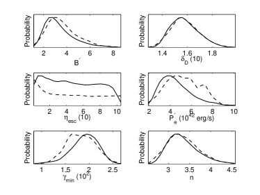
Figure 8: Same as Figure 6, but for the SEDs Periods G (Top) and H (Middle) reported in Hayashida et al.(2012).

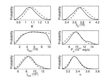
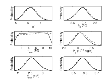
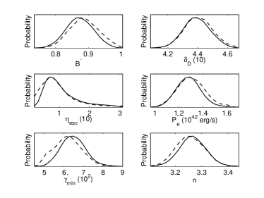
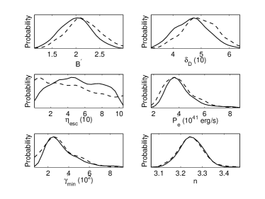
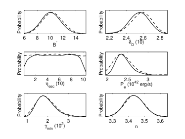
Figure 9: Same as Figure 6, but for the SEDs reported by Paliya et al.(2015). The plots from top to bottom are Flare1, Flare2 and post-flare, respectively.

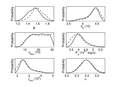
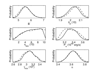
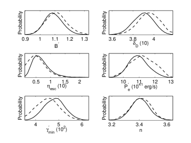
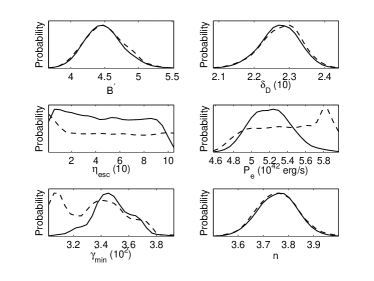
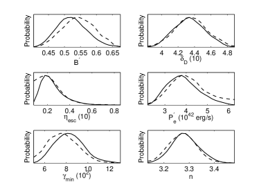
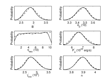
Figure 10: Same as Fig.6, but for the SEDs reported by Hayashida et al.(2015). The plots from top to bottom are Periods A, C and D, respectively.

The one-dimensional (1D) probability distributions of the free parameters are shown in Figures 6-10 in Appendix A. The uncertainties on the parameters in the two cases are given in Tables 1 and 2, respectively. We also report the marginalized 95% confidence intervals (CIs) of the parameters.

One can see that all parameters except for $\eta_{\rm esc}$ are well constrained. In the EC-DT model, $\eta_{\rm esc}$ in four states are well constrained (see Table 1). In the EC-BLR model, $\eta_{\rm esc}$ in all states are poorly constrained (see Table 2). The constraint on $\eta_{\rm esc}$ arises from the X-ray data. $\eta_{\rm esc}$ determines the minimum Lorenz factor in the emitting EED $\gamma_{\rm c}^{\prime}$, i.e., $\gamma^{\prime}_{\rm c}/|\dot{\gamma^{\prime}}(\gamma^{\prime}_{\rm c})|=\eta_{\rm esc}R^{\prime}/c$. $\gamma^{\prime}_{\rm c}$ has a big impact on the low energy part (X-ray band) of the EC component. If the EC emission contributes to the observed X-ray emission, $\gamma^{\prime}_{\rm c}$ or $\eta_{\rm esc}$ could be well constrained. In the EC-BLR model, the EC component peaks at higher energies, and the X-ray data are dominated by SSC emission. Therefore, $\eta_{\rm esc}$ is poorly constrained.

In addition, it is worth pointing out that our model fails to fit the $\gamma$-ray spectrum in the Period C in Hayashida et al. (2012), likely due to the simplification of the external photon fields. Complex external photon fields (Cerruti et al., 2013) may correct the discrepancy between the model and the data.

3.2 Injected EEDs

The injected EEDs obtained in the fittings are shown in the lower panels of Figures 1-4. It can be seen that the parameters describing the injected EEDs, i.e., $P^{\prime}_{e}$, $\gamma_{\rm min}^{\prime}$ and $n$, are well constrained. In the EC-DT model, $\gamma_{\rm min}^{\prime}$ is in the range from 248 to 877, and $P^{\prime}_{e}$ varies from $3.7\times 10^{41}$ to $3.9\times 10^{42}$ erg/s, and $n$ is in the range of $\sim 2.5-3.6$. It is noted that $n$ is larger than 3 except for the Periods A and B in Hayashida et al. (2012).

Looking at the injected EEDs and the emitting EEDs in Figures 1-4, one can find that the radiative cooling of the electrons occurs in the fast-cooling regime, i.e., $\gamma^{\prime}_{\rm c}<\gamma^{\prime}_{\rm min}$. In the fast cooling regime, $\gamma^{\prime}_{\rm min}$ is the break Lorentz factor of the emitting EED. The spectral index $s$ between $\gamma^{\prime}_{\rm c}$ and $\gamma^{\prime}_{\rm min}$ in steady-state emitting EED depends on the cooling rate of the electrons with $\gamma^{\prime}>\gamma^{\prime}_{\rm min}$. In the case of Thomson scattering or synchrotron energy-loss of the form $\dot{\gamma^{\prime}}\sim\gamma^{\prime 2}$, $s=2$. If the dominant energy-loss rate is not the form of $\dot{\gamma^{\prime}}\sim\gamma^{\prime 2}$ (e.g., IC in KN regime), $s$ should differ from 2 (see Yan et al., 2016b, for a detailed investigation on $s$ in different energy-loss processes in 3C 279). For the electrons with $\gamma^{\prime}>\gamma_{\rm min}^{\prime}$, the index of the distribution changes to be $n+1$, when the form of $\dot{\gamma}^{\prime}\propto\gamma^{\prime 2}$ holds.

It is noted that the EC-BLR model requires a larger injected electron power $P^{\prime}_{e}$, which is several times of that obtained in the EC-DT model. This is caused by the KN effect.

3.3 Properties of the $\gamma$-ray emission region

The magnetic field strength $B^{\prime}$ and the Doppler factor $\delta_{\rm D}$ are two important physical quantities. In Figures 6-10, it is found that the two quantities are constrained very well with the current data. In Table 1, one can see that $B^{\prime}$ varies in the range of [0.5-2.0] G, and $\delta_{D}$ varies in the range of [34.6-47.5]. With the values of $\delta_{D}$, we find that the values of $R^{\prime}$ are in the range of $\sim(4.8-6.6)\times 10^{15}$ cm. They are consistent with that derived in previous works (e.g., Dermer et al., 2014; Yan et al., 2016a) where static emitting EEDs were used. The large values of $\delta_{D}$ are also suggested by the VLBI study of the kinematics of the jet in 3C 279 (Lister & Marscher, 1997; Jorstad et al., 2004).

3.4 Correlations between model parameters and observed $\gamma$-rays

The model parameters as a function of the observed $\gamma$-ray flux $F_{\gamma}$ (Hayashida et al., 2012, 2015; Paliya et al., 2015) are showed in Figure 5. We calculate the Pearson’s probability for a null correlation, namely the p-value, which is reported in the corresponding panel of Figure 5.

Our results show that the $\gamma$-ray activity is tightly correlated with $P_{e}^{\prime}$ and $\gamma^{\prime}_{\rm min}$, with the p-values of $p=8.72\times 10^{-5}$ and $p=5.45\times 10^{-4}$, respectively. It indicates that the $\gamma$-ray activity is associated with the injection of the accelerated electrons.

In addition, there is a weak correlation between $F_{\gamma}$ and $\delta_{D}$, with $p=0.04$. No correlation between $F_{\gamma}$ and $B^{\prime}$ is found.

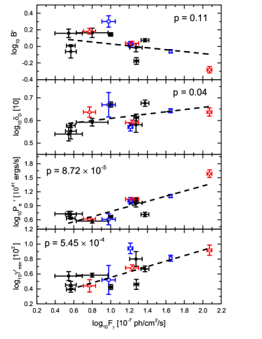
Figure 5: Evolutions of the model parameters ($B^{\prime}$, $\delta_{D}$, $\gamma_{\rm min}^{\prime}$, and $P_{e}^{\prime}$) as a function of the observed $\gamma$-ray flux $F_{\gamma}$. The black-dashed line is the linear best-fitting to the data. The red triangles, blue open squares and black filled squares are the results derived by fitting the three SEDs in Hayashida et al.(2015), the three SEDs in Paliya et al.(2015), and the eight SEDs in Hayashida et al.(2012), respectively.

3.5 Jet powers

Using the model parameters, we can derived the powers carried by the jet in the form of radiation ($L_{r}$), magnetic field ($L_{B}$), electrons ($L_{e}$) and protons ($L_{p}$) (e.g., Celotti & Fabian, 1993). However, the poorly constrained $\gamma^{\prime}_{\rm c}$ leads to large uncertainties on $L_{e}$ and $L_{p}$. Here, we calculate $L_{r}$ and $L_{B}$ using our well constrained parameters (Table 3). One can find $L_{r}\sim L_{B}$ except for the Period D in Hayashida et al. (2015).

The jet power $L_{\rm kin}$ can also be estimated by the $L_{\rm kin}-L_{151}$ relation obtained by Godfrey & Shabala (2013),

$$L_{\rm kin}=3\times 10^{44}\left(\frac{L_{151}}{10^{25}\rm W/Hz/sr}\right)^{0.67}~{}\rm erg/s,$$ (13)

where $L_{151}$ is the 151 MHz radio luminosity from the extended jet. The scaling relationship is roughly consistent with the theoretical relation presented in Willott et al. (1999). This approach is widely used to estimate the jet kinetic energy in AGNs.

Using the relation $L_{151}=d_{L}^{2}F^{151}$, we have $L_{\rm kin}=3\times 10^{44}(9.23F^{151})^{0.67}$ erg/s, where $F^{151}$ is in the units of Jy. With $F^{151}=22.08$ Jy (Arshakian et al., 2010), we obtain $L_{\rm kin}=1.05\times 10^{46}$ erg/s, which is dozens times of $L_{r}$.

4 Discussions

At first, we would like to stress that our model implicitly assumes a small acceleration zone which cannot contribute significant photons to the observed radiations.

4.1 On the acceleration mechanism

Obviously, the values of $n$ significantly depart from the canonical $n\simeq 2$ predicted by the non-relativistic shock acceleration, and also differ from $n\simeq 2.2$ expected by the classic relativistic shock acceleration (e.g., Kirk et al., 2000; Baring et al., 1999; Achterberg et al., 2001; Ellison & Double, 2004). Although a steeper distribution ($n\simeq 2.5$) can be produced considering the modification of shock by the back-reaction of the accelerated particles (e.g., Kirk et al., 1996), it still fails to account for the large values of $n$ we obtained.

Note that the above discussions are given in the frame of (quasi-)parallel shocks. Relativistic oblique shocks could produce much softer injection EED with $n>2.5$ (Ellison & Double, 2004; Niemiec & Ostrowski, 2004; Sironi & Spitkovsky, 2009; Summerlin & Baring, 2012). In relativistic shocks, Summerlin & Baring (2012) showed that the spectral index $n$ varies dramatically from 1 to $>3$ with the changes of obliquity and magnetic turbulence. Steep electron distribution with $n\sim 3$ can be produced in relativistic shocks with large obliquity and low turbulence. Therefore, our results indicate that the relativistic shocks with large obliquity and low turbulence may be responsible for the acceleration of electrons in 3C 279.

In relativistic shocks, the minimum Lorentz factor of the distribution is (e.g., Sari et al., 1998; Piran, 1999)

$$\gamma_{\rm min}^{\prime}\simeq\frac{m_{p}}{m_{e}}\frac{n-2}{n-1}\epsilon_{e}\Gamma_{\rm sh},~{}n>2$$ (14)

where $\Gamma_{\rm sh}$ is the bulk Lorentz factor across the shock front, and $\epsilon_{e}$ is the fraction of shock energy that goes into the electrons. From our results, we use $n=3.4$, $\gamma^{\prime}_{\rm min}=300$, and assume $\Gamma_{\rm sh}=10$ (Ushio et al., 2010), then we obtain $\epsilon_{e}\simeq 0.03$. This indicates that the acceleration is low-efficiency, which is consistent with the numerical simulation result in Sironi & Spitkovsky (2009).

The strongest evidence for an oblique shock can be found in the polarization maps of the jet emissions (Lind & Blandford, 1985; Cawthorne & Cobb, 1990; Cawthorne, 2006; Nalewajko, 2009; Nalewajko & Sikora, 2012). Abdo et al. (2010) discovered a dramatic change in the optical polarization associated with the $\gamma$-ray flare in Period D in Hayashida et al. (2012). They suggested that the observed polarization behavior may be the result of the jet bending. Jet bending has been observed in a number of AGNs (e.g., Graham & Tingay, 2014). In this scenario, an oblique shock could be formed due to the interaction of the jet with the external medium. Denn et al. (2000) have organized an extensive VLBI monitoring. They revealed the existent of the oblique shocks in the knots through the observed linear polarization behavior. Lister & Homan (2005) have shown that the distribution of the electric vector position angles (EVPA) offsets is similar to that predicted by an ensemble of oblique shocks with random orientations (Lister et al., 1998). Dulwich et al. (2009) have shown that the high-resolution data from the Very Large Array, Hubble Space Telescope and Chandra observatories support the presence of an oblique shock in the kiloparsec-scale jet of the powerful radio galaxy 3C 346. Very recently, some authors proposed that radio-to-$\gamma$-ray variabilities may be caused by the oblique shocks in AGN jets (Hughes et al., 2011; Hovatta et al., 2014; Aller et al., 2014; Hughes et al., 2015). In particular, Using a relativistic oblique shock acceleration + radiation-transfer model, Böttcher & Baring (2019) successfully explained the SEDs and variabilities of 3C 279 during flaring activity in the period December 2013 - April 2014 reported in Hayashida et al. (2015).

Our results show that the $\gamma$-ray activities strongly correlated with the injection of electrons. This indicates that the $\gamma$-ray activities could be caused by the acceleration of the electrons in the relativistic oblique shock.

4.2 On the Magnetization and Radiative Efficiency

The most promising scenario for launching blazar powerful jets involves the central accumulation of large magnetic flux and the formation of magnetically arrested/choked accretion flows (MACF) (Narayan et al., 2003; Igumenshchev, 2008; Tchekhovskoy et al., 2009, 2011; McKinney et al., 2012; Chen, 2018). In this scenario, the jet is powered by the Blandford-Znajek (BZ) mechanism that extracts BH rotational energy, and the jet production efficiency for maximal BH spin is estimated by $\eta_{j}\simeq 1.9(\phi_{\rm BH}/50)^{2}$ where $\phi_{\rm BH}$ is the dimensionless magnetic flux threading the BH (Blandford & Znajek, 1970; Tchekhovskoy et al., 2010; Sikora & Begelman, 2013; Sikora et al., 2013). The value of $\phi_{\rm BH}$ is typically on the order of 50 according to the numerical simulations by McKinney et al. (2012), although it depends on the details of the model.

Assuming $L_{\rm jet}=L_{\rm kin}$, one can find $\eta_{j}\equiv\epsilon L_{\rm jet}/L_{d}\simeq 1.6$ for $\epsilon=0.3$ (Thorne, 1974) and $L_{d}\sim 2\times 10^{45}$ erg/s (Pian, 1999). It is in good agreement with $\eta_{j}=1.9$ in the MCAF scenario for a typical value of $\phi_{\rm BH}=50$. Therefore, our result supports the BZ mechanism for jet launching

The magnetization and radiative efficiency are usually considered to be the indicator of acceleration mechanism occurring in blazar jets. We derive the magnetization parameter $\sigma_{B}$ and radiative efficiency $\eta_{r}$ (Kang et al., 2014; Sikora, 2016; Fan et al., 2018),

$$\sigma_{B} = L_{B}/(L_{\rm kin}-L_{B}),$$ (15)

$$\eta_{r} = L_{r}/(L_{\rm kin}+L_{r}).$$ (16)

Since $L_{\rm kin}$ is the time-averaged kinetic power of a source with the radio flux $F^{151}$, we use the average values of $L_{B}$ and $L_{r}$ and get $\sigma_{B}\simeq\eta_{r}\simeq 0.02$. Baring et al (2017) showed that electrons would be efficiently accelerated by relativistic shocks in blazar jets with $\sigma_{B}$ changing from $\sim 10^{-4}$ to 0.06.

5 Summary

Using a time-dependent one-zone SSC+EC model and the MCMC fitting technique, we analyzed 14 high-quality SEDs of 3C 279. We assume that the $\gamma$-ray emission region is either in the BLR or in the DT. The results show that the SEDs are better fitted in the latter case. The injected EED is well constrained in each state. The index of the injected EED is large, ranging from 2.7 to 3.8, which cannot be produced in (quasi-)parallel shocks. We argue that the steep injected EED may be the result of the acceleration of relativistic oblique shocks. According to the correlations of $F_{\gamma}$ and $\gamma_{\rm min}^{\prime}$, $P^{\prime}_{e}$, the $\gamma$-ray flares are caused by the acceleration.

Appendix A One-dimensional probability distributions of the free model parameters

Appendix B One-dimensional probability distributions of the derived parameters obtained from SED fittings with the DT photons

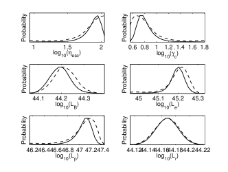
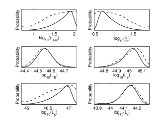
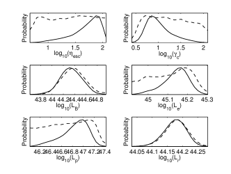
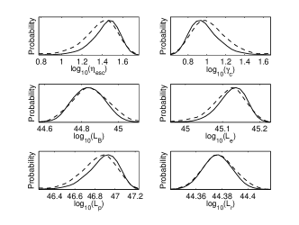
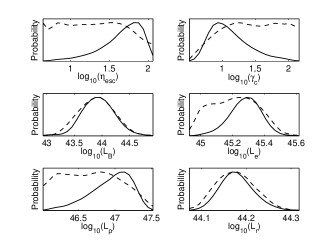
Figure 11: 1D probability distributions of the derived parameters in the EC-DT model. In the left panel, the plots from top to bottom are arranged in the following order Periods A, B, C and D reported in Hayashida et al.(2012), and Periods E, F, G and H are shown in the right panel.

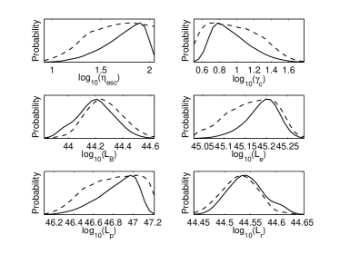
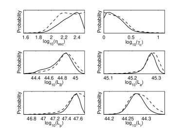
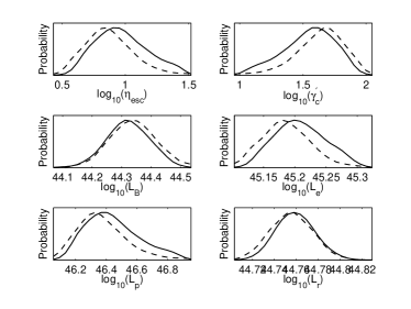
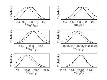
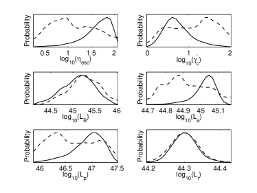
Figure 12: Same as Figure 11, but for the SEDs reported by Paliya et al.(2015) (Left) and the SEDs reported by Hayashida et al.(2015) (Right). In the left panel, the plots from top to bottom are Flare1, Flare2 and Post-Flare, respectively. In the right panel, the plots from top to bottom are Periods A, C and D, respectively.

References

- Abdo et al. (2010) Abdo A. A., Ackermann M., Ajello M., et al., 2010, Natur, 463, 919
- Abdo et al. (2011) Abdo A. A., Ackermann M., Ajello M., et al., 2011, ApJ, 736, 131
- Achterberg et al. (2001) Achterberg A., Gallant Y. A., Kirk J. G., Guthmann A. W., 2001, MNRAS, 328, 393
- Aller et al. (2014) Aller M. F., Hughes P. A., Aller H. D., Latimer G. E., Hovatta T., 2014, ApJ, 791, 53A
- Aleksic et al. (2015) Aleksić J. et al., 2015, A&A, 578, 22
- Arshakian et al. (2010) Arshakian T. G., Torrealba J., et al., 2010, A&A, 520A, 62A
- Baring et al. (1999) Baring M. G., Ellison D. C., Reynolds S. P., Grenier I. A., Goret P., 1999, ApJ, 513, 311
- Baring et al (2017) Baring M. G., Böttcher M., Summerlin E. J., 2017, MNRAS, 464, 4875
- Blumenthal & Gould (1970) Blumenthal G. R. Gould R. J., 1970, RvMP, 42, 237
- Blandford & Znajek (1970) Blandford R. D., Znajek R. L., 1977, MNRAS, 179, 433
- Blazejowski et al. (2000) Blazejowski M., Sikora M., Moderski R., Madejski G. M., 2000, ApJ, 545, 107
- Böttcher & Chiang (2002) Böttcher M. Chiang J., 2002, ApJ, 581, 127
- Böttcher et al. (2007) Böttcher M., Basu, S. Joshi, M. et al., 2007, ApJ, 670, 968
- Böttcher et al. (2013) Böttcher M., Reimer A., Sweeney K., Prakash A., 2013, ApJ, 768, 54
- Böttcher & Baring (2019) Böttcher M., Baring M. G., 2019, ApJ, 887, 133.
- Cawthorne & Cobb (1990) Cawthorne T. V. Cobb W. K., 1990, ApJ, 350, 536C
- Cawthorne (2006) Cawthorne T. V., 2006, MNRAS, 367, 851C
- Celotti & Fabian (1993) Celotti A., Fabian A. C., 1993, MNRAS, 264, 228
- Cerruti et al. (2013) Cerruti M., Dermer C. D., Lott B., Boisson C., Zech A., 2013, ApJL, 771, L4
- Chiaberge & Ghisellini (1999) Chiaberge M. Ghisellini G., 1999, MNRAS, 306, 551
- Chen (2018) Chen L., 2018, ApJS, 235, 39
- Coppi et al (1990) Coppi P. S. Blandford R. D., 1990, MNRAS, 245, 453
- Collmar et al. (2010) Collmar W., Böttcher M., Krichbaum T. P., et al., 2010, A&A, 522, A66
- Denn et al. (2000) Denn G. R., Mutel R. L., Marscher A. P., 2000, ApJS, 129, 61
- Dermer et al. (2009) Dermer C. D., Fink J. D., Krug H., Böttcher M., 2009, ApJ, 692, 32
- Dermer et al. (2014) Dermer C. D., Cerruti M., Lott B., Boisson C., Zech A., 2014, ApJ, 782, 82
- Drury et al. (1983) Drury L. O’C., 1983, Rep. Prog. Phys., 46, 973
- Dulwich et al. (2009) Dulwich F., Worrall D. M., Birkinshaw M., et al., 2009, MNRAS, 398, 1207D
- Ellison et al (1990) Ellison D. C., Jones F. C., Reynolds S. P., 1990, ApJ, 360, 702
- Ellison & Double (2004) Ellison D. C., Double G. P., 2004, Astropart. Phys., 22, 323
- Fan et al. (2018) Fan Xu-Liang, Wu Qingwen, Liao, Neng-Hui, 2018, ApJ, 861, 97
- Finke et al. (2008) Finke J. D., Dermer C. D., Böttcher M., 2008, ApJ, 686, 181
- Ghisellini & Tavecchio (2008) Ghisellini G. Tavecchio F., 2008, MNRAS, 387, 1669
- Ghisellini & Tavecchio (2009) Ghisellini G., Tavecchio F., 2009, MNRAS, 397, 985
- Ghisellini et al. (2010) Ghisellini G., Tavecchio F., Foschini L., et al., 2010, MNRAS, 402, 497
- Godfrey & Shabala (2013) Godfrey L. E. H., Shabala S. S., 2013, ApJ, 767, 12
- Graff et al. (2008) Graff P. B., Georganopoulos M., et al., 2008, ApJ, 689, 68G
- Graham & Tingay (2014) Graham P. J., Tingay S. J., 2014, ApJ, 784, 159
- Guo et al. (2015) Guo F., Liu Y. H., Daughton W., Li H., 2015, ApJ, 806, 167
- Hartman et al. (1996) Hartman R. C., et al., 1996, ApJ, 461, 698
- Hayashida et al. (2012) Hayashida M., Madejski G. M., Nalewajko K. et al., 2012, ApJ, 754, 114
- Hayashida et al. (2015) Hayashida M., Nalewajko K., Madejski G. et al., 2015, ApJ, 807, 79
- Hovatta et al. (2014) Hovatta Talvikki, Aller Margo F., et al., 2014, AJ, 147, 143H
- Hu et al. (2015) Hu W., Fan Z. H., Dai, B. Z., 2015, RAA, 15, 1455
- Hu et al. (2017b) Hu W., Zeng W., Dai B. Z., 2017b, arXiv1711.05494
- Hughes et al. (2011) Hughes Philip A., Aller Margo F., Aller Hugh D., 2011, ApJ, 735, 81H
- Hughes et al. (2015) Hughes Philip A., Aller Margo F., Aller Hugh D., 2015, ApJ, 799, 207H
- Igumenshchev (2008) Igumenshchev I. V., 2008, ApJ, 677, 317
- Jones (1968) Jones F. C., 1968, PhRv, 167, 1159J
- Jones & Ellison (1991) Jones F. C., Ellison D. C., 1991, Space Sci. Rev., 58, 259
- Jorstad et al. (2004) Jorstad S. G., Marscher A. P., Lister M. L., et al., 2004, AJ, 127, 3115
- Kang et al. (2014) Kang S. J., Chen L., Wu Q., 2014, ApJS, 215, 5
- Kirk & Heavens (1989) Kirk J. G., Heavens A. F., 1989, MNRAS, 239, 995
- Kirk et al. (1996) Kirk J. G., Duffy P., Gallant Y. A., 1996, A&A, 314, 1010
- Kirk et al. (2000) Kirk J. G., Guthmann A. W., Gallant Y. A., Achterberg A., 2000, ApJ, 542, 235
- Lewis & Bridle (2002) Lewis A., Bridle, S., 2002, Phys. Rev. D, 66, 103511
- Lind & Blandford (1985) Lind K. R., Blandford R. D., 1985, ApJ, 295, 358
- Lister & Marscher (1997) Lister M. L., Marscher A. P., 1997, ApJ, 476, 572
- Lister et al. (1998) Lister M. L., Marscher A. P., Gear W. K., 1998, ApJ, 504, 702
- Lister & Homan (2005) Lister M. L., Homan D. C., 2005, AJ, 130, 1389L
- Liu et al. (2012) Liu J., Yuan Q., Bi X. J., Li H., Zhang X.M., 2012, Phys. Rev. D, 85, d3507
- Liu & Bai (2006) Liu H. T., Bai J. M., 2006, ApJ, 653, 1089L
- Massaro et al. (2006) Massaro E., Tramacere A., Perri M., Giommi P., Tosti G., 2006, A&A, 448, 861
- McKinney et al. (2012) McKinney J. C., Tchekhovskoy A., Blandford R. D., 2012, MNRAS, 423, 3083
- Narayan et al. (2003) Narayan R., Igumenshchev I. V., Abramowicz M. A., 2003, PASJ, 55, L69
- Nalewajko (2009) Nalewajko K., 2009, MNRAS, 395, 524N
- Nalewajko & Sikora (2012) Nalewajko K., Sikora M., 2012, A&A, 543A, 115N
- Niemiec & Ostrowski (2004) Niemiec J., Ostrowski M., 2004, ApJ, 610, 851
- Pacciani et al. (2014) Pacciani L., Tavecchio F., Donnarumma I., et al., 2014, ApJ, 790, 45
- Paliya et al. (2015) Paliya V. S., Sahayanathan S., Stalin C. S., 2015, ApJ, 803, 15
- Peng et al. (2014) Peng Ya-ping, Yan Da-hai, Zhang Li, 2014, MNRAS, 442, 2357
- Pian (1999) Pian E., Urry C. M., Maraschi L., et al., 1999, ApJ, 521, 112
- Piran (1999) Piran T., 1999, PhR, 314, 575
- Poole et al. (2008) Poole T. S., Breeveld A. A., Page M. J., et al., 2008, MNRAS, 383, 627P
- Sari et al. (1998) Sari R., Piran T., Narayan R., 1998, ApJL, 497, L17
- Sikora et al. (1994) Sikora M., Begelman M. C., Rees M. J., 1994, ApJ, 421, 153
- Sikora & Begelman (2013) Sikora M., Begelman M. C., 2013, ApJL, 764, L24
- Sikora et al. (2013) Sikora M., Stasińska G., Kozieł-Wierzbowska D., Madejski G. M., Asari N. V., 2013, ApJ, 765, 62
- Sikora (2016) Sikora M., 2016, Galax, 4, 12
- Sironi & Spitkovsky (2009) Sironi L., Spitkovsky A., 2009, ApJ, 698, 1523
- Sironi et al. (2015) Sironi L., Keshet U., Lemoine M., 2015, SSRv, 191, 519
- Stickel et al. (1991) Stickel M., Padovani P., Urry C. M., Fried J. W., Kuehr H., 1991, ApJ, 374, 431
- Stocke et al. (1991) Stocke J. T., Morris S. L., Gioia I. M., et al., 1991, ApJS, 76, 813
- Summerlin & Baring (2012) Summerlin E. J., Baring M. G., 2012, ApJ, 745, 63
- Tavecchio & Ghisellini (2008) Tavecchio F., Ghisellini G., 2008, MNRAS, 386, 945T
- Tchekhovskoy et al. (2009) Tchekhovskoy A., McKinney J. C., Narayan R., 2009, ApJ, 699, 1789
- Tchekhovskoy et al. (2010) Tchekhovskoy A., Narayan R., McKinney J. C., 2010, ApJ, 711, 50
- Tchekhovskoy et al. (2011) Tchekhovskoy A., Narayan R., McKinney J. C., 2011, MNRAS, 418, L79
- Thorne (1974) Thorne K. S., 1974, ApJ, 191, 507
- Tramacere et al. (2011) Tramacere A., Massaro E., Taylor A. M., 2011, ApJ, 739, 66
- Ulrich et al. (1997) Ulrich M. H., Maraschi L., Urry C. M., 1997, ARA&A, 35, 445
- Urry & Padovani (1995) Urry C. M., Padovani P., 1995, PASP, 107, 803
- Ushio et al. (2010) Ushio M., Stawarz Ł., Takahashi T., et al., 2010, ApJ, 724, 1509
- Wehrle et al. (1998) Wehrle A. E., et al., 1998, ApJ, 497, 178
- Willott et al. (1999) Willott C. J., Rawlings S., Blundell K. M., Lacy M., 1999, MNRAS, 309, 1017
- Wu et al. (2018) Wu Lin-hui, Wu Qingwen, Yan Da-hai, et al., 2018, ApJ, 852, 45
- Yan et al. (2013) Yan D. H., Zhang L., Yuan Q., Fan Z. H., Zeng H. D., 2013, ApJ, 765, 122
- Yan et al. (2015) Yan D. H., Zhang L., Zhang S. N., 2015, MNRAS, 454, 1310
- Yan et al. (2016a) Yan D. H., He J. J., Liao J. Y. et al., 2016a, MNRAS, 456, 2173
- Yan et al. (2016b) Yan D. H., Zhang L. Zhang S. N., 2016b, MNRAS, 459, 3175
- Yuan et al. (2011) Yuan Q., Liu S., Fan Z., Bi X., Fryer C., 2011, ApJ, 735, 120
- Zhang et al. (2012) Zhang J., Liang E. W., Zhang S. N., Bai J. M., 2012, ApJ, 752, 157
- Zhou et al (2014) Zhou Y., Yan D. H., Dai B. Z., Zhang, L., 2014, PASJ, 66, 12