Abstract

Kronecker Products (KP) have been used to compress IoT RNN Applications by 15-38x compression factors, achieving better results than traditional compression methods. However when KP is applied to large Natural Language Processing tasks, it leads to significant accuracy loss (approx 26%). This paper proposes a way to recover accuracy otherwise lost when applying KP to large NLP tasks, by allowing additional degrees of freedom in the KP matrix. More formally, we propose doping, a process of adding an extremely sparse overlay matrix on top of the pre-defined KP structure. We call this compression method doped kronecker product compression. To train these models, we present a new solution to the phenomenon of co-matrix adaption (CMA), which uses a new regularization scheme called co-matrix dropout regularization (CMR). We present experimental results that demonstrate compression of a large language model with LSTM layers of size 25 MB by 25$\times$ with 1.4% loss in perplexity score. At 25$\times$ compression, an equivalent pruned network leads to 7.9% loss in perplexity score, while HMD and LMF lead to 15% and 27% loss in perplexity score respectively.

1 Introduction

The large size of Natural Language Processing (NLP) applications can make it impossible for them to run on resource constrained devices with limited memory and cache budgets Thakker et al. (2019c); Tao et al. (2019). Fitting these applications into IoT devices requires significant compression. For example, to fit a 25 MB Language Model on an IoT device with 1 MB L2 Cache, requires 25x compression or 96% reduction in the number of parameters. Recently, Kronecker Products (KP) were used to compress IoT applications by 15-38x compression factors Thakker et al. (2019d; b) and achieves better accuracy than pruning Zhu & Gupta (2017), low-rank matrix factorization (LMF) and small baseline (SB). However, when we apply KP to a large language modeling (LM) application, we see a 26% loss in accuracy at 338x compression. Unlike pruning (amount of sparsity) and LMF (rank of the matrix), there is no obvious method to control the amount of compression of the KP compressed network. Thakker et al. (2019b) propose Hybrid KP (HKP) to solve this issue. HKP helps recover the lost accuracy by injecting more parameters in the KP compressed network. However, the compression factor reduces to 5x to bring down the accuracy loss within 1.5% loss in baseline perplexity.

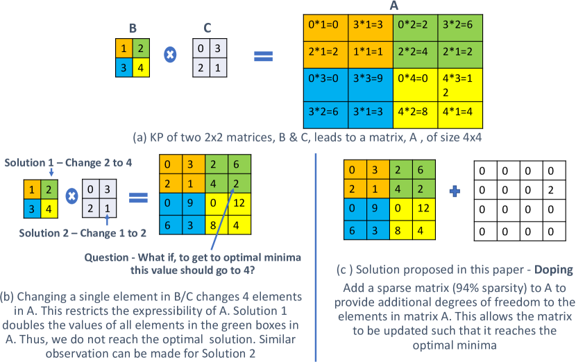
Figure 1: (a) Example of a Kronecker Product of two matrices. (b) Issues with back-propagation through a matrix expressed as a KP of two smaller matrices. (c) Shows how doping solves the issues discussed in (b)

This paper explores another method to inject parameters into a KP compressed network. This method is based on the observations that parameters in the KP space need additional degrees of freedom (Figure 1 a,b). Inspired by robust PCA techniques, we propose adding a sparse matrix to a KP compressed matrix in order to facilitate these additional degrees of freedom (Figure 1 c). Thus, a parameter matrix in an RNN, LSTM, GRU, or Transformer layer is replaced by a sum of two matrices – one expressed as a KP of two smaller matrices ($M_{kp}$) and the other an extremely sparse matrix ($M_{sp}$). During training, $M_{sp}$ starts off with 0% sparsity. Over time, we prune the unimportant weights in the $M_{sp}$ matrix to get to the required amount of sparsity. These pruned values will represent the equivalent values in $M_{kp}$ that did not require the additional degrees of freedom. This methodology of compression is called Doped Kronecker Product (DKP) in this paper. However, training DKP compressed networks is non-trivial and requires overcoming co-matrix adaption (CMA) (Section 3.1) using a specialized regularization scheme (Section 3.3).The preliminary results using this compression scheme are encouraging. We show that we can compress the medium sized LM in Zaremba et al. (2014) by 25$\times$ with 1.2% loss in perplexity score, improving perplexity of pruned Zhu & Gupta (2017) network by to 6.7%, HMD Thakker et al. (2019a) by 13.8% and LMF Kuchaiev & Ginsburg (2017) by 25.8%.

In the rest of the paper, we discuss the CMA issues associated with a general doping mechanism (3.1), some methods to overcome CMA based on popular training techniques (3.2), the technique proposed in this paper to overcome CMA (3.3), results of compressing a medium LM using DKP and comparison against popular compression techniques and previously published work (4)

2 Related Work

The research in NN compression can be broadly categorized under 4 topics - Pruning Han et al. (2016); Zhu & Gupta (2017), structured matrix based techniques Sindhwani et al. (2015); Thakker et al. (2019b; d); Gope et al. (2020a), quantization Hubara et al. (2016); Courbariaux & Bengio (2016); Gope et al. (2020b; 2019) and tensor decomposition Tjandra et al. (2017). DKP combines pruning and structured matrix based techniques and compares the results with pruning, structured matrix and tensor decomposition based compression techniques. The networks compressed using this technique can be further compressed using quantization.

3 Doped Kronecker Product (DKP) Compression

Table 1: Results of compressing using DKP when a matrix is expressed as shown in equation 1

Baseline Perplexity	82.04
Compression Factor	$338\times$	$100\times$
Sparsity of $M_{sp}$	100%	99.93%
DKP Perplexity	104	138.3

DKP expresses a matrix as a sum of a $M_{kp}$ and a sparse matrix -

$$W=B\otimes C+M_{sp}$$ (1)

The sparsity of $M_{sp}$ determines the amount of compression. For example, if W is of size 100$\times$100, B and C are of size 10$\times$10, then 95% sparsity in $M_{sp}$ will lead to 14$\times$ compression and 90% sparsity in $M_{sp}$ will lead to 8.4$\times$ compression. During the initial phase of training, $M_{sp}$ is dense. As training progresses, $M_{sp}$ reaches the required sparsity level. Thus we allow back-propagation to determine which elements of the $M_{kp}$ matrix ($B\otimes C$) require additional degrees of freedom.

3.1 Co-matrix Adaptation (CMA)

Figure 2: Graph of training perplexity vs training epochs and sparsity of $M_{sp}$ matrix vs training epoch for the medium LM at 100$\times$ compression factor. As the sparsity of $M_{sp}$ matrix increases, the training perplexity degrades. This indicates that the NN is too reliant on the $M_{sp}$ matrix during the initial phase of the training process and less reliant on the $M_{kp}$ matrix. We call this phenomenon as co-matrix adaptation.

Equation 1 is one way to implement DKP and represents our initial attempt at compressing using DKP. We compressed the LSTM layers in the medium LM in Zaremba et al. (2014) using this method. The LM has 2 LSTM layers with hidden vector of size 650. This creates matrices of size $2600\times 1300$ amounting to a total size of 25 MB. We compress these layers by 25$\times$ by replacing the matrices in the LSTM layers as shown in equation 1. By adding a $M_{sp}$ with 99% sparsity, the perplexity score degrades by 32.9%. Thus adding 1% more parameters to $M_{kp}$ leads to poorer perplexity score than baseline. Figure 2 shows the graph of training perplexity vs training epochs and sparsity of $M_{sp}$ matrix vs training epoch for the medium LM at 100$\times$ compression factor. As the sparsity of $M_{sp}$ matrix increases, the training perplexity degrades. This indicates that the LM is too reliant on the $M_{sp}$ matrix during the initial phase of the training process when the matrix is dense and less reliant on the $M_{kp}$ matrix. When the $M_{sp}$ becomes extremely sparse, $M_{kp}$ is no longer able to pull the perplexity score back. We suspect that this might be because the model is stuck in a local minima dictated by the dense $M_{sp}$ matrix. We will refer to this phenomena as co-matrix adaptation (CMA).

The phenomenon of CMA is more clearer when we focus on the number of back-propagation updates during the initial phase of training. The $M_{kp}$ matrix is composed of the kronecker product of two matrices of size $13\times 65$ and $50\times 20$ leading to a total of 9980 parameters. While the $M_{sp}$ matrix in its initial dense form has a total of 3382600 parameters. Thus, during back-propagation, $M_{sp}$ matrix receives $339\times$ more updates than the $M_{kp}$ matrix. This might sway the NN to find a minima that is too reliant on the parameters of the $M_{sp}$ matrix. As a result, when the training progresses and the $M_{sp}$ matrix is pruned, the accuracy drops significantly.

3.2 Overcoming CMA

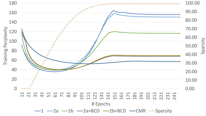
Figure 3: Using the various techniques described in equation 2a - 2b with and without BCD, we see that the reliance on $M_{sp}$ has reduced. The increase in training perplexity that was visible in 2 has been managed considerably.

Table 2: Test Perplexity of DKP compressed medium LM for various training techniques discussed in Section 3.2 and 3.3. CMR techniques leads to the best accuracy for 100$\times$ compression factor.

Compression Factor	Training Method	Sparsity of $M_{sp}$	Test Perplexity
1x	Baseline	NA	82.04
$338\times$	2a	0	104.061
$100\times$	1	99.93	150.737
	2a	99.93	138.31
	2b	99.93	123.835
	2a+BCD	99.93	100.37
	2b+BCD	99.93	101.987
	CMR	99.93	95.382

Table 3: Results of compressing medium LM over multiple compression factors using DKP, HMD, HKP, LMF, Pruning and Small Baseline

Baseline Test Perplexity	82.04
Compression Factor	$338\times$	$100\times$	$92\times$	$75\times$	$50\times$	$25\times$	$20\times$	$10\times$	$5\times$
DopedKP	104.061	95.49	86.576	86.73	85.45	83.24	82.94	82.9	82.53
Prune	115.62	103.219	103.34	91.618	90.314	88.555	85.14	82.551	82.47
HKD	Did not run						99.882	95.12	92.56
HMD							105.43	97.59	95.387
LMF							108.61	103.42	99.29
Small Baseline							115.34	109.78	102.2

The key to overcoming CMA is to reduce the reliance on $M_{sp}$ initially. This paper explored multiple avenues to do so.

$$W =B\otimes C+\beta\times M_{sp},min\left\lVert\beta\right\rVert$$ (2a)

$$\begin{split}W=\alpha\times(B\otimes C)+\beta\times M_{sp},\\ min(\left\lVert\beta\right\rVert+\left\lVert 1/\alpha\right\rVert)\end{split}$$ (2b)

Each of the equations 2a - 2b can be further trained with or without Block Coordinate Descent (BCD). In BCD we alternate between, only training $M_{kp}$, blocking gradient flow to $M_{sp}$, or train $M_{kp}$, blocking gradient flow to $M_{sp}$. The training curves across multiple epochs for these various techniques can be found in Figure 3. As the sparsity increases, the training perplexity does not increase as much as in figure 2 for equations 2a-2b when trained using BCD. However, there is still a small increase in training error with increased sparsity. This can indicate that CMA may have not been completely managed. Table 2 shows the test perplexity at the end of training for the various techniques discussed above. As you can see, these techniques help us bring the perplexity down to 100.37 from 150.737 originally. However, by reducing the compression factor from $338\times$ to $100\times$, we are improving the perplexity by approximately $4$ points only.

3.3 Co-matrix Row Dropout Regularization (CMR)

To better manage CMA, we focused on how a DKP Cell converts input feature vector into an output feature vector. When an input feature vector, $i$, is fed to a LSTM layer, it gets multiplied with the weight matrix,

$$o=W*i.$$ (3)

In the case of DKP, $W$ is composed of two sets of matrices

$$o=(M_{kp}+M_{sp})*i,\mbox{where }M_{kp}=B\otimes C\\$$ (4)

$$o=M_{kp}*i+M_{sp}*i$$ (5)

Thus each element of the output vector is a combination of output of $M_{kp}*I$ and $M_{sp}*I$, i.e.

$$o_{j:}=(M_{kp})_{j:}*i+(M_{sp})_{j:}*i$$ (6)

where $j:$ refers to the $j^{th}$ row of the $M_{kp}$ and $M_{sp}$ matrix. Thus each element (or neuron) of the output feature vector is the sum of elements (or neurons) coming in from the $M_{kp}$ matrix and the $M_{sp}$ matrix.

Our hypothesis is that during CMA, the incoming neurons from the $M_{kp}$ matrix and the $M_{sp}$ matrix learn to co-adapt, leading to lost capacity. Furthermore, because of the dominance of the $M_{sp}$ matrix during the initial phase of the training (Section 3.1), the $M_{kp}$ neurons rely on the $M_{sp}$ neurons heavily. If we introduce a stochastic behavior where either the $M_{kp}$ neuron or the $M_{sp}$ neuron are not available to drive the output neuron, this co-adaptation could be managed. Thus to manage CMA more efficiently, this paper proposes co-matrix row dropout regularization (CMR). This regularization extends the concept of stochastic depth Huang et al. (2016) to regularize the output of each row of the output vector in order to avoid CMA. From a mathematical point of view, we introduce dropout after the output of each $M_{kp}*i$ and $M_{sp}*$ value, i.e. equation 6 is changed to,

$$o_{j:}=((M_{kp})_{j:}*I)bern_{1}+((M_{sp})_{j:}*I)*bern_{2},$$ (7)

where,

$$bern_{1},bern_{2}\sim Bernoulli\{p\}.$$ (8)

As the sparsity of $M_{sp}$ increases, the need for CMR decreases and can be removed entirely. The training methodology described by equation 7 is referred to as CMR in this paper. CMR is an extremely effective technique to manage CMA as evident by the trends in Figure 3 for CMR. The training perplexity during the training phase does not increase as the sparsity of the $M_{sp}$ matrix increases. The benefits in the final Test Perplexity are also evident as shown in the last row of the Table 2.

4 Results

Table 4: Comparing DKP with previous published work targeting the same benchmark

Comparisons with prior art	Compression Factor	Test Perp
Baseline LM	$1\times$	82.04
4-bit quant Park et al. (2017)	$8\times$	83.84
3-bit quant Lee & Kim (2018)	$10.67\times$	83.14
Tensor Train Grachev et al. (2019)	$1.67\times$	168.639
Weight Distortion Lee et al. (2018)	$10\times$	84.64
Weight Distortion Lee et al. (2018)	$20\times$	93.39
DKP (Ours)	$25\times$	83.24

We compress the PTB based medium LM in Zaremba et al. (2014) by multiple compression factors and compare the DKP trained using CMR with pruning (Zhu & Gupta (2017)), LMF (Kuchaiev & Ginsburg (2017)), HMD (Thakker et al. (2019c)) and HKP (Thakker et al. (2019b)). As a baseline, we also train a small baseline by reducing the size of the hidden vector in the LSTM layer.

Table 3 shows the results of compressing the benchmark for various compression factors. As shown, DKP outperforms all compression techniques up to $20\times$ compression factors. Table 4 further compares these results with other recently published work. Again, our compression technique outperforms these recent papers, achieving $2.5\times$ more compression than the best performing technique.

5 Conclusion

This paper presents a new compression technique called Doped Kronecker Product (DKP). However, training DKP is non-trivial and can run into co-matrix adaptation issues. We further propose co-matrix row dropout regularization (CMR) to manage CMA. The preliminary results demonstrate that using DKP with CMR, we can compress a large language model with LSTM layers of size 25 MB by 25$\times$, with 1.2% loss in perplexity score. Our technique outperforms popular compression techniques in previously published work, improving the perplexity scores by 7.9% - 27%.

References

- Courbariaux & Bengio (2016) Courbariaux, M. and Bengio, Y. Binarynet: Training deep neural networks with weights and activations constrained to +1 or -1. CoRR, abs/1602.02830, 2016. URL http://arxiv.org/abs/1602.02830.
- Gope et al. (2019) Gope, D., Dasika, G., and Mattina, M. Ternary hybrid neural-tree networks for highly constrained iot applications. In Proceedings of Machine Learning and Systems 2019, pp. 190–200. 2019.
- Gope et al. (2020a) Gope, D., Beu, J., Thakker, U., and Mattina, M. Ternary mobilenets via per-layer hybrid filter banks. In Proceedings of the IEEE/CVF Conference on Computer Vision and Pattern Recognition (CVPR) Workshops, June 2020a.
- Gope et al. (2020b) Gope, D., Beu, J. G., Thakker, U., and Mattina, M. Aggressive compression of mobilenets using hybrid ternary layers. tinyML Summit, 2020b. URL https://www.tinyml.org/summit/abstracts/Gope_Dibakar_poster_abstract.pdf.
- Grachev et al. (2019) Grachev, A. M., Ignatov, D. I., and Savchenko, A. V. Compression of recurrent neural networks for efficient language modeling. CoRR, abs/1902.02380, 2019. URL http://arxiv.org/abs/1902.02380.
- Han et al. (2016) Han, S., Mao, H., and Dally, W. J. Deep compression: Compressing deep neural networks with pruning, trained quantization and huffman coding. International Conference on Learning Representations (ICLR), 2016.
- Huang et al. (2016) Huang, G., Sun, Y., Liu, Z., Sedra, D., and Weinberger, K. Q. Deep networks with stochastic depth. CoRR, abs/1603.09382, 2016. URL http://arxiv.org/abs/1603.09382.
- Hubara et al. (2016) Hubara, I., Courbariaux, M., Soudry, D., El-Yaniv, R., and Bengio, Y. Quantized neural networks: Training neural networks with low precision weights and activations. CoRR, abs/1609.07061, 2016. URL http://arxiv.org/abs/1609.07061.
- Kuchaiev & Ginsburg (2017) Kuchaiev, O. and Ginsburg, B. Factorization tricks for LSTM networks. CoRR, abs/1703.10722, 2017. URL http://arxiv.org/abs/1703.10722.
- Lee & Kim (2018) Lee, D. and Kim, B. Retraining-based iterative weight quantization for deep neural networks. CoRR, abs/1805.11233, 2018. URL http://arxiv.org/abs/1805.11233.
- Lee et al. (2018) Lee, D., Kapoor, P., and Kim, B. Deeptwist: Learning model compression via occasional weight distortion. CoRR, abs/1810.12823, 2018. URL http://arxiv.org/abs/1810.12823.
- Park et al. (2017) Park, E., Ahn, J., and Yoo, S. Weighted-entropy-based quantization for deep neural networks. In 2017 IEEE Conference on Computer Vision and Pattern Recognition (CVPR), pp. 7197–7205, July 2017. doi: 10.1109/CVPR.2017.761.
- Sindhwani et al. (2015) Sindhwani, V., Sainath, T., and Kumar, S. Structured transforms for small-footprint deep learning. In Cortes, C., Lawrence, N. D., Lee, D. D., Sugiyama, M., and Garnett, R. (eds.), Advances in Neural Information Processing Systems 28, pp. 3088–3096. Curran Associates, Inc., 2015.
- Tao et al. (2019) Tao, J., Thakker, U., Dasika, G., and Beu, J. Skipping rnn state updates without retraining the original model. In Proceedings of the 1st Workshop on Machine Learning on Edge in Sensor Systems, SenSys-ML 2019, pp. 31–36, New York, NY, USA, 2019. Association for Computing Machinery. ISBN 9781450370110. doi: 10.1145/3362743.3362965. URL https://doi.org/10.1145/3362743.3362965.
- Thakker et al. (2019a) Thakker, U., Beu, J. G., Gope, D., Dasika, G., and Mattina, M. Run-time efficient RNN compression for inference on edge devices. CoRR, abs/1906.04886, 2019a. URL http://arxiv.org/abs/1906.04886.
- Thakker et al. (2019b) Thakker, U., Beu, J. G., Gope, D., Zhou, C., Fedorov, I., Dasika, G., and Mattina, M. Compressing rnns for iot devices by 15-38x using kronecker products. CoRR, abs/1906.02876, 2019b. URL http://arxiv.org/abs/1906.02876.
- Thakker et al. (2019c) Thakker, U., Dasika, G., Beu, J. G., and Mattina, M. Measuring scheduling efficiency of rnns for NLP applications. CoRR, abs/1904.03302, 2019c. URL http://arxiv.org/abs/1904.03302.
- Thakker et al. (2019d) Thakker, U., Fedorov, I., Beu, J. G., Gope, D., Zhou, C., Dasika, G., and Mattina, M. Pushing the limits of RNN compression. CoRR, abs/1910.02558, 2019d. URL http://arxiv.org/abs/1910.02558.
- Tjandra et al. (2017) Tjandra, A., Sakti, S., and Nakamura, S. Compressing recurrent neural network with tensor train. In Neural Networks (IJCNN), 2017 International Joint Conference on, pp. 4451–4458. IEEE, 2017.
- Zaremba et al. (2014) Zaremba, W., Sutskever, I., and Vinyals, O. Recurrent neural network regularization. CoRR, abs/1409.2329, 2014. URL http://arxiv.org/abs/1409.2329.
- Zhu & Gupta (2017) Zhu, M. and Gupta, S. To prune, or not to prune: exploring the efficacy of pruning for model compression. arXiv e-prints, art. arXiv:1710.01878, October 2017.