The Hubble Space Telescope UV Legacy Survey of Galactic Globular Clusters. XX. Ages of single and
multiple stellar populations in seven bulge globular clusters

Abstract

In the present work we analyzed seven globular clusters selected from their location in the Galactic bulge and with metallicity values in the range $-1.30\lesssim\rm{[Fe/H]}\lesssim-0.50$. The aim of this work is first to derive cluster ages assuming single stellar populations, and secondly, to identify the stars from first (1G) and second generations (2G) from the main sequence, subgiant and red giant branches, and to derive their age differences. Based on a combination of UV and optical filters used in this project, we apply the Gaussian mixture models to distinguish the multiple stellar populations. Applying statistical isochrone fitting, we derive self-consistent ages, distances, metallicities, and reddening values for the sample clusters. An average age of $12.3\pm 0.4$ Gyr was obtained both using Dartmouth and BaSTI (accounting atomic diffusion effects) isochrones, without a clear distinction between the moderately metal-poor and the more metal-rich bulge clusters, except for NGC 6717 and the inner halo NGC 6362 with $\sim 13.5$ Gyr. We derived a weighted mean age difference between the multiple populations hosted by each globular cluster of $41\pm 170$ Myr adopting canonical He abundances; whereas for higher He in 2G stars, this difference reduces to $17\pm 170$ Myr, but with individual uncertainties of $500$ Myr.

1 Introduction

The early formation and present configuration of the Galactic bulge is complex, and studies of its stellar populations can give hints on its formation and evolution processes (Barbuy et al., 2018a). Globular clusters (GCs) are tracers of the formation and chemodynamical evolution of the Milky Way (MW). In particular, the bulge GCs are witnesses of the earliest stages of the Galaxy formation. As an example, the old age of $\sim 13$ Gyr derived for some of the moderately metal-poor bulge GCs with a blue horizontal branch, in particular NGC 6522, NGC 6626 and HP 1 (Kerber et al., 2018, 2019), suggest that they were formed before the present configuration of the bulge/bar component (Renzini et al., 2018), considering that the Galactic bar was recently estimated to have an age of $8\pm 2$ Gyr (Buck et al., 2018; Bovy et al., 2019).

The Hubble Space Telescope (HST) UV Legacy Survey of Galactic GCs (GO-13297 program, PI G. Piotto; Piotto et al., 2015, hereafter Paper I of this series) allowed to obtain photometry for 56 GCs with the UV/blue filters F275W, F336W and F438W of the Ultraviolet and Visual Channel of the Wide Field Camera 3 (UVIS/WFC3). The main goals of this survey are to identify and investigate the nature of the multiple stellar populations (MPs) in GCs. The bandpasses of this “magic trio” of filters include the OH, NH, CN and CH molecular bands (Paper I), thus showing the C, N and O abundance variations, as detected in spectroscopy (e.g. Gratton et al., 2012). Previous data in optical filters (F606W and F814W), obtained with the Advanced Camera for Surveys (ACS), the Survey of Galactic GCs (GO-10775 program, PI A. Sarajedini; Sarajedini et al., 2007), are also available.

In the present work, we analyze the seven bulge GCs observed in these HST programs that are within the selection of bulge GCs by Bica et al. (2016): NGC 6304, NGC 6352, NGC 6624 and NGC 6637 (M69), with literature metallicities in the range $-0.75\lesssim\rm{[Fe/H]}\lesssim-0.35$; and NGC 6652, NGC 6717 (Pal 9) and NGC 6723, with $-1.25\lesssim\rm{[Fe/H]}\lesssim-0.75$ (Harris, 1996, 2010 edition; Carretta et al. 2009). They are located at Galactic latitudes $|b|\leq 17\mbox{$.\!^{\circ}$}50$ and Galactocentric distances $R_{\rm GC}\leq 3.3$ kpc, therefore within the bulge volume, and they are a representative sample of the moderately metal-rich and moderately metal-poor bulge GCs. In a recent classification from orbital analysis by Pérez-Villegas et al. (2020), the GCs NGC 6304, NGC 6624, NGC 6637 and NGC 6717 are confirmed as bulge members. NGC 6352 has a higher probability to be part of the thick disk for a high bar speed, whereas for the case of slow bar pattern speed it could also have a significant probability to be part of the bulge; NGC 6723 and NGC 6652 would belong to the thick disk. The old inner halo cluster NGC 6362, recently studied by Kerber et al. (2018) in terms of ages, and by Mucciarelli et al. (2016) and Massari et al. (2017) in terms of spectroscopic abundances, was also selected for comparison purposes.

Accurate age determinations for GCs depend on high-precision photometry and are indeed a great challenge, particularly for those in the Galactic bulge, due to the combination of high field stellar contamination, strong total and differential extinction, and also stellar crowding effects normally present in any GC. Recent efforts have been made by using the HST in the visible and near-infrared (NIR), NIR detectors assisted by adaptive optics (AO) systems in $8-10$ m class telescopes and, when possible, proper-motion (PM) cleaning techniques to overcome these obstacles (e.g. Cohen et al., 2014, 2018; Lagioia et al., 2014; Correnti et al., 2016, 2018; Ferraro et al., 2016; Saracino et al., 2016, 2019; Kerber et al., 2018, 2019).

The reliability of age derivations require a statistical and self-consistent analysis to be applied to deep and multiband color-magnitude diagrams (CMDs), such as those provided among the more recent ones, by the HST UV Legacy Survey of Galactic GCs (Piotto et al., 2015), the ACS Survey of Galactic GCs (Sarajedini et al., 2007) and the WFC3/NIR survey of GCs toward the Galactic bulge (Cohen et al., 2018).

Absolute and relative ages were determined for 69 GCs using the ACS Survey of Galactic GCs data (Sarajedini et al., 2007), applying different isochrone fitting methods and theoretical models (Marín-Franch et al., 2009; Dotter et al., 2010; VandenBerg et al., 2013; Wagner-Kaiser et al., 2017). The bulge GC NGC 6352 was analyzed in detail by Nardiello et al. (2015, Paper IV). In the present work we carry out a detailed analysis for the seven sample bulge GCs, including NGC 6352.

As concerns MP analyses, the first detections of anomalous abundances of light elements from proton-capture processes were presented in the 1970s (e.g. Osborn, 1971), but no theories about MPs were developed yet, because the evidence was restricted to evolved giant stars. For a few clusters, in particular M22 and $\omega$ Centauri, evidence on metallicity variations were suggested (e.g. Pilachowski et al., 1982; Hesser et al., 1977) – see also photometric evidence from Lee et al. (1999), but these clusters are considered to be special cases until today. Since the first photometric evidence of MPs among unevolved stars of GCs with HST by Bedin et al. (2004) and Piotto et al. (2005), the observations have been showing that the phenomenon is common to almost all GCs so far studied. Reviews on the evidence revealing chemical abundance anomalies can be found in Kraft (1994) and Gratton et al. (2012). Reviews on photometric evidence of MPs were presented by Piotto (2009), and more recently by Bastian & Lardo (2018, and references therein).

Renzini et al. (2015, Paper V) describe the possible scenarios for 2G formation from the ejected material processed by 1G stars, including massive asymptotic giant branch (AGB) stars, massive interacting binaries and fast-rotating massive stars. These models predict age differences between 1G and 2G going from about zero (for the supermassive star model, e.g. Gieles et al., 2018), to $\lesssim 30$ Myr (for the massive rotating star model, see e.g. Decressin et al., 2007), to about $50-100$ Myr (for the AGB model, e.g. D’Ercole et al., 2008) and possibly up to $\sim 150$ Myr (D’Antona et al., 2016) for the Type II clusters (Paper IX). Although none of the scenarios can reproduce all the observational evidence, a reliable determination of the age differences between MPs might turn out to favor one or some of them. Therefore, an extremely accurate determination of age differences, of less than 1% of the cluster ages, would be needed to constrain the models. This level of precision cannot be reached for old clusters, and it might be feasible by analysing younger clusters, although other problems (e.g. rotation) may arise to hamper accurate determinations (e.g. D’Antona et al., 2017; Milone et al., 2018a).

In this work, the ages, metallicities, distance moduli and reddening values are derived via isochrone fitting following a Bayesian approach, assuming both the single and multiple stellar populations. The MPs are identified from the main sequence (MS) to the red giant branch (RGB). Theoretical stellar evolutionary models with canonical He abundances and $\alpha$-enhancement, from A Bag of Stellar Tracks and Isochrones (BaSTI, Pietrinferni et al., 2006) and Dartmouth Stellar Evolutionary Database (DSED, Dotter et al., 2008) were adopted. The isochrone fitting was carried out in membership probability cleaned CMDs with optical filters.

The high precision in the relative age derivations from our isochrone fitting method allows us to investigate a possible age difference between the MPs, otherwise impossible with higher uncertainties. In Paper IV the relative ages between the MPs in NGC 6352 were derived, obtaining an age difference of $10\pm 110$ Myr and a He abundance variation of $\Delta Y=0.029\pm 0.006$, assuming no difference in $\rm{[Fe/H]}$ and $\rm{[\alpha/Fe]}$. However, adopting a small variation in $\rm{[Fe/H]}$ and $\rm{[\alpha/Fe]}$, the uncertainty in the age difference rises to 280 Myr.

In Section 2, the GO-13297 observations are briefly described. Section 3 presents the statistical methods for isochrone fitting, following a Bayesian approach. In Section 4, the isochrone fits considering the sample GCs as a single stellar population (SSP) are shown. Section 5 presents the separation of their MPs and the age derivation for each generation. In Section 6, conclusions are drawn.

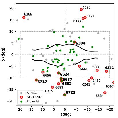
Figure 1: Location in Galactic coordinates of the GCs presented in Harris (1996, 2010 edition) catalog, within $|\ell|<22\arcdeg$ and $|b|<22\arcdeg$. The open red circles correspond to the 56 GCs observed in the GO-13297 program. The black contours correspond to the COBE/DIRBE outline of the peanut bulge (Weiland et al., 1994; Jönsson et al., 2017), and the dashed lines delimit the central region with $|\ell|<20\arcdeg$ and $|b|<10\arcdeg$. The only six clusters with $R_{\rm GC}<3$ kpc and $\rm{[Fe/H]}>-1.5$, classified as bulge GCs in Bica et al. (2016, green circles), were selected for this present analysis. NGC 6352, which is classified as an outer bulge GC, was also selected.

Table 1: Cluster parameters and metallicity from Harris (1996, 2010 edition, H10), other metallicity values from Carretta et al. (2009, C09) and Vásquez et al. (2018, V18), HB color differences from Dotter et al. (2010) and masses from Baumgardt & Hilker (2018). The horizontal lines in the following tables divide the bulge GCs from the inner halo one.

Cluster	$\ell$	$b$	$d_{\odot}$	$R_{\rm GC}$	$E(B-V)$	$\rm{[Fe/H]}_{\rm{H10}}$	$\rm{[Fe/H]}_{\rm{C09}}$	$\rm{[Fe/H]}_{\rm{V18}}$	$\Delta(V-I)$	Mass
	(deg)	(deg)	(kpc)	(kpc)	(mag)	(dex)	(dex)	(dex)	(mag)	($10^{5}$ M⊙)
NGC 6304	355.83	5.38	5.9	2.3	0.54	$-0.45$	$-0.37$	$-0.43\pm 0.05$	$0.105$	2.61
NGC 6352	341.42	$-7.17$	5.6	3.3	0.22	$-0.64$	$-0.62$	$-0.54\pm 0.03$	$0.123$	0.596
NGC 6624	2.79	$-$7.91	7.9	1.2	0.28	$-0.44$	$-0.42$	$-0.37\pm 0.01$	$0.135$	0.930
NGC 6637	1.72	$-$10.27	8.8	1.7	0.18	$-0.64$	$-0.59$	$-0.48\pm 0.02$	$0.138$	1.63
NGC 6652	1.53	$-11.38$	10.0	2.7	0.09	$-0.81$	$-0.76$	$-0.82\pm 0.07$	$0.141$	0.521
NGC 6717	12.88	$-10.90$	7.1	2.4	0.22	$-1.26$	$-1.26$	$-1.17\pm 0.09$	$0.948$	0.181
NGC 6723	0.07	$-17.30$	8.7	2.6	0.05	$-1.10$	$-1.10$	$-1.01\pm 0.06$	$0.371$	1.69
NGC 6362	25.55	$-17.57$	7.6	5.1	0.09	$-0.99$	$-1.07$	$-1.03\pm 0.06$	$0.247$	1.13

Table 2: Metallicity and chemical abundances derived from high-resolution spectroscopy of individual stars from the literature.

Cluster	[Fe/H]	[O/Fe]	[Na/Fe]	[Al/Fe]	[Mg/Fe]	[Si/Fe]	[Ca/Fe]	[Ti/Fe]	[Ba/Fe]	[$\alpha$/Fe]	Ref.
NGC 6352	$-0.55\pm 0.03$	—	$+0.18$	$+0.32$	$+0.47$	$+0.20$	$+0.19$	$+0.15$	—	$+0.20$	F09
NGC 6624	$-0.69\pm 0.02$	$+0.41$	—	$+0.39$	$+0.42$	$+0.38$	$+0.40$	$+0.37$	—	$+0.39$	V11
NGC 6637	$-0.77\pm 0.02$	$+0.20$	$+0.35$	$+0.49$	$+0.28$	$+0.45$	$+0.20$	$+0.24$	$+0.22$	$+0.27^{\dagger}$	L07
NGC 6723	$-0.98\pm 0.08$	$+0.29$	$+0.00$	$+0.31$	$+0.23$	$+0.36$	$+0.30$	$+0.24$	+0.22	$+0.28^{\dagger}$	R16
	—	$+0.39$	$+0.05$	—	$+0.52$	—	—	—	—	$+0.46^{\dagger}$	G15a
	$-1.22\pm 0.01$	$+0.53$	$+0.13$	—	$+0.51$	$+0.60$	$+0.81$	—	$+0.75$	$+0.61^{\dagger}$	G15b
	$-0.93\pm 0.05$	$+0.39$	$+0.14$	$+0.32$	$+0.47$	$+0.52$	$+0.37$	$+0.34$	$+0.36$	$+0.39$	C19
NGC 6362	$-1.09\pm 0.01$	—	+0.00	—	—	—	—	—	—	—	M16a
	$-1.09\pm 0.01$	—	+0.33	—	—	—	—	—	—	—	M16b
	$-1.07\pm 0.01$	—	—	$+0.51$	$+0.54$	$+0.45$	$+0.26$	$+0.24$	+0.61	$+0.32$	M17

Note. — F09: Feltzing et al. (2009);V11: Valenti et al. (2011); L07: Lee (2007); R16: Rojas-Arriagada et al. (2016); G15: Gratton et al. (2015) for blue (G15^a) and red (G15^b) HB stars; C19: Crestani et al. (2019); M16: Mucciarelli et al. (2016) for 1G (M16^a) and 2G (M16^b) stars; M17: Massari et al. (2017). ^†The $\alpha$-element abundances which were not made explicit in the references were computed here as the mean of O, Mg, Si, Ca and Ti abundances, if available. NGC 6304, NGC 6652 and NGC 6717 are not included in any high-resolution spectroscopic study of individual stars.

2 Observations: GO-13297 program

The objective of the GO-13297 program is the identification of MPs in a sample of 56 GCs (the most central of them in the Galaxy are identified in Figure 1), using the WFC3/UVIS UV and blue filters F275W, F336W and F438W. The exposure times were set up to reach a color precision of $0.02$ mag in F275W just below the main-sequence turnoff (MSTO). Paper I presented the exposure times and observing strategies adopted. Previous photometry with the ACS/WFC F606W and F814W optical filters (GO-10775, Sarajedini et al., 2007) was also obtained for this sample.

The $2.6\arcmin\times 2.6\arcmin$ field of view of WFC3 is slightly smaller than that of ACS/WFC ($3.4\arcmin\times 3.4\arcmin$) and therefore GO-13297 data target a more central region of the GCs. The data reduction pipelines (adapted from Anderson et al., 2008) and the astro-photometric catalogs used in this work are described in Paper I and Nardiello et al. (2018, Paper XVII). We adopted the same procedure described in Paper XVII for selecting the well-measured stars, based on the photometric errors and two quality parameters for the five HST filters.

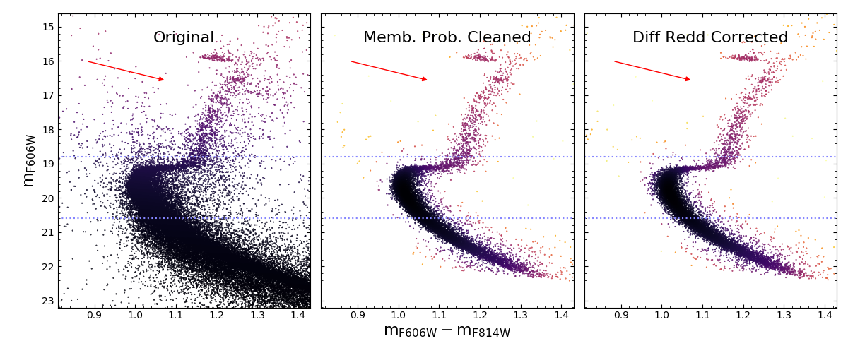
Figure 2: Example of the CMD cleaning process for NGC 6304. The left panel shows the original $m_{\rm F606W}$ vs. $m_{\rm F606W}-m_{\rm F814W}$ CMD, the middle panel shows the membership probability cleaned CMD, and the right panel shows the final CMD after applying also the differential reddening correction. The dotted-blue lines enhance the most age-sensitive region in the CMD, whose stars are actually used in our isochrone fitting method. The relative PMs used to calculate the membership were measured combining GO-10775 and GO-13297 photometry ($\Delta\mathrm{t}=7-8$ yr). A reddening vector of $E(B-V)=0.20$ is given by the red arrow.

The photometry was also corrected for differential reddening (DR) as in Milone et al. (2012a) and decontaminated from field stars via membership-probability cleaning (Paper XVII). The DR correction is crucial for age derivation, since the reddening vector is almost perpendicular to the subgiant branch (SGB) and MSTO. The original CMD and those resulting from the membership-probability and DR-cleaning processes are shown in Figure 2 for the moderately metal-rich cluster NGC 6304, which has the largest reddening in our sample.

2.1 The sample

The GO-10775 and GO-13297 programs covered only a few outer bulge objects (Figure 1), essentially because they focused on nearby GCs with low reddening values, to ensure the feasibility of observations in a few HST orbits. The distribution of the central GCs in Galactic coordinates presented in Figure 1 justifies the sample selection: among the 20 observed clusters within $|b|<22\arcdeg$ and $|\ell|<22\arcdeg$, only six of them have $R_{\rm GC}\lesssim 3$ kpc and $\rm{[Fe/H]}>-1.5$, classified as bulge GCs, in Bica et al. (2016). We also include NGC 6352 which is slightly farther, at 3.3 kpc from the Galactic center.

The twin clusters NGC 6388 and NGC 6441 were not analyzed because they are characterized by an extremely blue horizontal branch morphology despite their quite high metallicity (Rich et al., 1997; Busso et al., 2007). Besides, they are classified as type-II and type-I ambiguous respectively, by Milone et al. (2017, Paper IX), making their stellar populations even more difficult to be disentangled. Bellini et al. (2013) carried out a multicolor analysis with HST filters to detect their MPs.

Table 1 presents the coordinates and photometric parameters of the sample clusters from Harris (1996, 2010 edition) and mass from Baumgardt & Hilker (2018). Literature metallicity values from Carretta et al. (2009) and Vásquez et al. (2018), according to the updated compilation by Dias et al. (2015, 2016), are included. In Table 2 are reported the metallicities and chemical abundances derived from high-resolution spectroscopy, available in the literature. Figures 2 and 3 show the $m_{\rm F606W}$ vs. $m_{\rm F606W}-m_{\rm F814W}$ membership and DR-cleaned CMDs of the sample clusters. Appendix A presents an overview of previous literature work for these GCs.

In a previous work in this series, Milone et al. (2017, Paper IX) provided an atlas of MPs in all the 56 GCs, extracting the so-called “chromosome maps” to perform a uniform analysis and determine the fraction of 1G stars. We have followed the same steps to disentangle the RGB and MS stellar populations, together with the method described in Paper IV to separate the SGB stellar populations. The analysis of the multiple populations in this paper is carried out in Section 5.

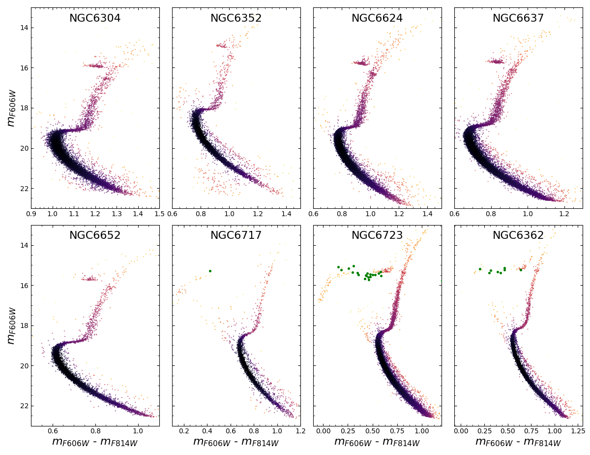
Figure 3: Membership probability and differential reddening cleaned CMDs of the seven bulge GCs and the reference halo one NGC 6362. The upper panels show the moderately metal-rich, and the lower panels show the moderately metal-poor GCs. Green points in the last panels show the cataloged RR Lyrae stars that returned a cross-match with this HST photometry (Section 3.3).

Brown et al. (2016, Paper VII) analyzed the HB morphology of the sample clusters, showing that the four moderately metal-rich GCs are dominated by red clump stars (NGC 6304, NGC 6352, NGC 6624 and NGC 6637), as well as the slightly more metal-poor NGC 6652; the most metal-poor has an extended blue horizontal branch (NGC 6717); and the two remaining have intermediate morphologies (NGC 6362 and NGC 6723). The color difference $\Delta(V-I)$ between the HB and RGB, from Dotter et al. (2010), is listed in Table 1 and agrees with these HB morphologies. Milone et al. (2014) also carried out a similar analysis, but with the F606W and F814W HST filters.

Milone et al. (2018b, Paper XVI) have shown that the average He difference between the 2G and 1G stars does not exceed 0.010 in mass fraction for the sample GCs (and maximum internal variation below 0.030); considering all the 56 GCs, the average enhancement is also of $\sim 0.010$. It is consistent with Lagioia et al. (2018, Paper XII), where an average He enhancement of $0.011\pm 0.002$ in 2G stars was derived from an analysis of the RGB bump in 18 GCs.

3 Isochrone fitting method

The physical parameters of the GCs were determined by statistical comparisons between the observed stars (in a limited magnitude range from the MS to the RGB) and theoretical models. We have followed the basis of analysis previously presented by Kerber et al. (2007). Here, we use the SIRIUS code (Statistical Inference of physical paRameters of sIngle and mUltiple populations in Stellar clusters – Souza et al., 2020), with the aim of having a uniform and self-consistent method for age derivation via statistical isochrone fitting. It follows a Bayesian approach with the Markov chain Monte Carlo (MCMC) sampling method, in order to derive ages, distances, metallicity and reddening values for stellar clusters. In this work, SIRIUS is applied to the sample clusters as a single stellar population, as well as to their 1G and 2G stars separately.

The likelihood function is computed for each star $i$, relative to the $j^{th}$ closest point of each isochrone defined as the combination of four free parameters (age, $\rm{[Fe/H]}$, $E(B-V)$ and $(m-M)_{0}$), through:

$$L\propto\prod_{i=1}^{\rm{N}}\max\left\{\prod_{j=1}^{\rm{M}}\exp{\left(-\chi_{\rm{mag,j,i}}^{2}-\chi_{\rm{col,j,i}}^{2}\right)}\right\}\;,$$ (1)

where $mag$ refers to $m_{\rm F606W}$, $col$ is the color $m_{\rm F606W}-m_{\rm F814W}$ and $\sigma$ correspond to the uncertainties. The chi-squares $\chi_{\rm{mag,j,i}}^{2}$ and $\chi_{\rm{col,j,i}}^{2}$ are given by:

$$\ \chi_{\rm{mag,j,i}}^{2}=\frac{\left(mag_{i}-mag_{j}\right)^{2}}{\sigma_{\rm{mag,i}}^{2}}$$ (2)

$$\ \chi_{\rm{col,j,i}}^{2}=\frac{\left(col_{i}-col_{j}\right)^{2}}{\sigma_{\rm{col,i}}^{2}}\;.$$ (3)

In order to take into account the number of stars in each evolutionary stage, we apply a factor inversely proportional to the star count inside a small region around each star, in the likelihood function. The contribution of all $N$ stars are combined computing the natural logarithm ($\mathcal{L}=\ln L$), relatively to the $j$-th closest point of the isochrone with M points:

$$\mathcal{L}\propto\sum_{i=1}^{\rm{N}}\max\left\{-\sum_{j=1}^{\rm{M}}\left(\chi_{\rm{col,j,i}}^{2}+\chi_{\rm{mag,j,i}}^{2}\right)\right\}\;.$$ (4)

Thus, Gaussian distributions are assumed for the magnitude and color distributions of stars, following the evolutionary path given by the isochrone. The higher is the $\mathcal{L}$ value, the greater is the plausibility that a model represents the observation. The MCMC sampling is carried out using the emcee package (Foreman-Mackey et al., 2013) to simulate stochastic chains according to a number of walkers and steps. Some similar isochrone fitting methods have been applied recently. For instance, Kerber et al. (2018) applied a similar likelihood function, but comparing synthetic and observed fiducial lines instead of considering all stars. SIRIUS was already applied in Kerber et al. (2019) and Ortolani et al. (2019).

3.1 Stellar Evolutionary Models

Two sets of $\alpha$-enhanced isochrones are compared with the membership probability cleaned CMDs of the sample clusters:

• Dartmouth Stellar Evolutionary Database (DSED, Dotter et al., 2008);

• A Bag of Stellar Tracks and Isochrones (BaSTI, Pietrinferni et al., 2006).

All available ages (from 10.0 to 15.0 Gyr, in steps of 0.5 Gyr) and metallicity values were considered. Besides, we downloaded interpolated DSED isochrones in the online interpolator and performed linear interpolations in the original BaSTI isochrones, to build a more complete grid in [Fe/H] (steps of $0.01$ dex) and ages (0.1 Gyr), for the sake of a higher stability in the simulated chains.

Considering the results of Paper XII and Paper XVI, we assume here that the typical helium enhancement between MPs should not exceed $\sim 0.01$. Therefore, in the analysis of CMDs as SSPs, we adopt isochrones with a standard He abundance of $Y\sim 0.25$. See Section 5.3 for calculations with an ad hoc helium content for the MPs hosted by the globular clusters.

The BaSTI $\alpha$-enhanced models adopted in the present investigation do not account for atomic diffusion. Recently the BaSTI database has been updated by also accounting for the effects of atomic diffusion (Hidalgo et al., 2018). However, being this updated library available only for scaled-solar heavy elements distribution and being the updated $\alpha$-enhanced sets of models still under-construction, we have decided for the present investigations to rely on the previous BaSTI database. This notwithstanding, since the updated BaSTI models for the scaled-solar case have been computed for different assumption about the atomic diffusion efficiency (see Hidalgo et al., 2018, for details), we have adopted a subset of these new BaSTI models in order to properly estimate the impact of GC age dating of alternatively using model predictions accounting or not accounting for diffusive processes.

By comparing suitable, self-consistent isochrones we have estimated that using non-diffusive theoretical isochrones implies an overestimate of the cluster age by 0.80 Gyr in the metallicity range of our sample GCs. Therefore, the isochrone fits were carried out with the original BaSTI isochrones (Pietrinferni et al., 2006), and for the sake of clarity the offset of $0.80$ Gyr was included in the BaSTI solutions, represented in the text and tables hereafter by BaSTI*.

We have adopted the UV/optical photometric data (F275W, F336W and F438W filters) to properly tag and separate the individual MPs in the sample GCs, and subsequently we use only the optical bands F606W and F814W to derive ages. This is because UV filters are sensitive to the peculiar abundances of light elements characteristic of 2G stars, while optical bands are only sensitive to the He enhancement via its effect on the stellar effective temperature scale (see Sbordone et al., 2011; Cassisi et al., 2013; Milone et al., 2012b, 2018b). It would be extremely difficult and computing demanding to compute model atmospheres and, hence, suitable bolometric corrections for the relevant photometric passbands, accounting for each individual chemical patterns observed in 2G stars in the selected GC sample.

3.2 T_eff-dependent reddening corrections

Given that the extinction in the sample bulge GCs is rather high ($A_{V}\lesssim 1.60$), a second-order reddening correction must be applied to the isochrones, due to the extinction dependency on the effective temperature (Bedin et al., 2005). Sirianni et al. (2005) described in detail the corrections for HST/ACS CCD detectors, increasingly important for wider and bluer filters.

We apply this correction along the DSED and BaSTI models, by using PAdova and TRieste Stellar Evolution Code (PARSEC, Bressan et al., 2012) isochrones including interstellar extinction. Isochrones with $A_{\rm V}=0.00$ and $1.55$ are compared for each value of $T_{\rm eff}$, and the differences in magnitude between them are fitted to a quadratic function as a function of $T_{\rm eff}$. Figure 4 shows the derived $A_{\lambda}/A_{V}$ variation for the filters F606W ($\sim 5\%$) and F814W ($\sim 3\%$), used in the isochrone fitting. For the sake of completeness, we present the derived functions for the five HST bands, where $x=\log T_{\rm eff}$:

$$A_{\rm F275W}/A_{V}=-9.302x^{2}+70.336x-131.021$$ (5)

$$A_{\rm F336W}/A_{V}=-0.895x^{2}+6.777x-11.165$$ (6)

$$A_{\rm F438W}/A_{V}=-0.065x^{2}+0.590x+0.037$$ (7)

$$A_{\rm F606W}/A_{V}=-0.320x^{2}+2.552x-4.152$$ (8)

$$A_{\rm F814W}/A_{V}=-0.174x^{2}+1.347x-2.008$$ (9)

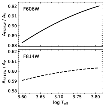
Figure 4: $A_{\rm F606W}/A_{V}$ and $A_{\rm F814W}/A_{V}$ variations as a function of the stellar effective temperature.

In the $m_{\rm F606W}$ versus $m_{\rm F606W}-m_{\rm F814W}$ CMD, these corrections have the effect of steepening the slope of the RGB and MS by $\Delta(m_{\rm F606W}-m_{\rm F814W})\sim 0.02$ and $0.03$ respectively. Kerber et al. (2018) derived a similar value of $\Delta(m_{\rm F435W}-m_{\rm F625W})\sim 0.05$. Assuming this correction is a linear function of the reddening, the coefficients of the derived functions for $A_{V}=1.55$ (Equations 5 to 9) are weighted for the desired $A_{V}$ value.

3.3 Prior distributions

In order to better constrain the free parameters during the isochrone fitting processes, we adopted the following set of prior distributions: canonical He content, non-negative $E(B-V)$, $\rm{[Fe/H]}$ from spectroscopic studies, and apparent distance modulus $(m-M)_{V}$ from RR Lyrae mean magnitudes, when available. The age was the only free parameter with a flat prior distribution.

Table 3 provides the Gaussian prior distributions employed in the metallicity for each cluster. For NGC 6352, NGC 6624, NGC 6637 and NGC 6362, the central values come from high-resolution spectroscopy and we assumed 3$\sigma$ as the uncertainty (see Table 2). Although NGC 6723 has high-resolution spectroscopic studies, the metallicity determinations are discrepant and an average value was adopted as the prior. For NGC 6304 and NGC 6652, the metallicity was derived only from integrated spectra in the literature (Conroy et al., 2018), therefore we used the values given in Table 1 with $\pm 0.15$ dex. There are no high-resolution spectroscopic studies for individual stars for NGC 6717, and we adopted the value from Carretta et al. (2009) with a $\sim 10\%$ uncertainty.

The luminosity-metallicity ($M_{V}-\rm{[Fe/H]}$) relation derived from RR Lyrae stars (RRLs) by Muraveva et al. (2018), together with the mean magnitudes of the cluster RRLs, allow us to obtain a reliable and independent constraint on the apparent distance modulus $(m-M)_{V}$. For each random set of parameters, the $E(B-V)$ value corresponds to a respective prior in the absolute distance modulus $(m-M)_{0}$.

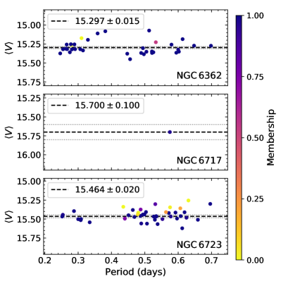
Figure 5: Mean $V$ magnitudes vs. period of the RRLs in the fields that contain NGC 6362, NGC 6717 and NGC 6723. The derived membership probabilities are represented by the color bar and the weighted averages are shown in each panel.

Using the catalogs from Clement et al. (2001, 2017 edition) and OGLE Collection of Variable Stars (OCVS, Soszyński et al., 2014), we retrieved the coordinates and magnitude of the RRLs located in a radius of $10\arcmin$ around the cluster center. NGC 6304 was the only cluster inside the OGLE covered area in the Galactic bulge. The catalogs contain 21 RRLs for NGC 6304, 4 for NGC 6652, 43 for NGC 6723, 35 for NGC 6362 and one RRL for each of the other GCs. Moreover, 3 red variables with unknown type and period are listed for NGC 6352. The Gaia DR2 catalog of RR Lyrae (Gaia Collaboration et al., 2018a) was checked in the fields around the sample GCs, but no new RR Lyrae were found.

The proper motions of all these RRLs were retrieved from Gaia DR2 (Gaia Collaboration et al., 2016, 2018a) data, by cross-matching coordinates. The Gaussian mixture models (GMM) were implemented in order to identify cluster and field stars, adjusting two Gaussian both for the right ascension and declination PMs. A membership probability was computed for each RRL using the equations from Bellini et al. (2009), which consider the measured PMs of this RRL, the cluster and the field, and their respective uncertainties.

The membership information given in the Paper XVII catalogs cannot be applied to the selected RRLs, since many of them are outside the $2.6\arcmin\times 2.6\arcmin$ WFC3 field of view. To illustrate this fact, Figure 3 presents the RRLs that returned a cross-match with the adopted HST catalogs, showing that around half of the original RRLs are located inside the WFC3 covered area. In turn, the RRLs detected in the cross-match populate exactly the instability strip region.

Figure 6: Mean magnitudes versus $(m-M)_{\rm{V}}$ of the RRLs in NGC 6362, NGC 6717 and NGC 6723. The apparent distance moduli (green circles) are given by the intersection of the $M_{\rm{V}}$$-$$\rm{[Fe/H]}$ relation (from Muraveva et al., 2018, M18, red diagonal lines), evaluated for the respective $\rm{[Fe/H]}$, and the average of the RRL mean magnitudes (black horizontal lines). The central values and uncertainties are represented by the solid and the dashed lines. The panels cover the same interval in $x$-axis and have the same scale in $y$-axis.

The membership analysis shows that only NGC 6362, NGC 6717 and NGC 6723 have RR Lyrae member stars. If a limit is set in $P_{i}\geq 75\%$, NGC 6362 contains 32 member RRLs, NGC 6723 contains 35 RRLs and NGC 6717 remains with its unique RRL. Salinas et al. (2019) report the discovery of new variable stars in NGC 6652, but no new RRLs; furthermore, one of the four cataloged RRLs was selected by them as a member, but our membership analysis concluded that its PM is not compatible with the derived values for the cluster stars.

In Figure 5 are shown the RRL mean magnitudes $\langle V\rangle$ versus period for NGC 6362, NGC 6717 and NGC 6723. The dashed line indicates the weighted average and standard deviation of $\langle V\rangle$ and the colors indicate the membership value of the RRLs, according to the color bar. The RRLs with low membership values ($P_{i}\leq 75\%$) were not excluded from the weighted average and standard deviation calculations, since its membership probability was used as the weight ($\overline{\langle V\rangle}=\sum\langle V\rangle_{i}P_{i}/\sum P_{i}$).

Relations $M_{V}-\rm{[Fe/H]}$ with slightly different slopes are found in the literature (e.g. Sandage, 1993; Clementini et al., 2003; Gaia Collaboration et al., 2017). In this work we adopted the recent Bayesian calibration derived by Muraveva et al. (2018), by using 381 local RRLs with accurate Gaia DR2 parallaxes (Gaia Collaboration et al., 2018a) together with photometric data (Dambis et al., 2013):

$$\ M_{V}=(0.34\pm 0.03)\cdot\rm{[Fe/H]}+(1.17\pm 0.04)\;.$$ (10)

Therefore, the absolute magnitude was computed according to the metallicity in Table 3 and, combined with the mean apparent magnitude of the sample RRLs, the apparent distance modulus was estimated and used as a prior. Figure 6 presents the intersection between the average of the observed mean magnitudes and the empirical $M_{V}-\rm{[Fe/H]}$ calibration, providing the expected $(m-M)_{V}$ (green circles, Table 3).

Table 3: Priors on metallicity, based on Table 2, and apparent distance modulus, applied for isochrone fitting.

Cluster	$\rm{[Fe/H]}$	$\langle V\rangle$	$(m-M)_{V}$
NGC 6304	$-0.45\pm 0.15$	—	—
NGC 6352	$-0.55\pm 0.09^{\dagger}$	—	—
NGC 6624	$-0.69\pm 0.06^{\dagger}$	—	—
NGC 6637	$-0.77\pm 0.06^{\dagger}$	—	—
NGC 6652	$-0.85\pm 0.15$	—	—
NGC 6717	$-1.26\pm 0.10$	$15.7\pm 0.1$	$14.96\pm 0.12$
NGC 6723	$-1.10\pm 0.10$	$15.464\pm 0.020$	$14.67\pm 0.07$
NGC 6362	$-1.07\pm 0.03^{\dagger}$	$15.297\pm 0.015$	$14.49\pm 0.05$

Note. — ^†A 3-$\sigma$ deviation from high-resolution measurement uncertainties was adopted in the prior.

Since only three GCs have member RRLs, the prior in $(m-M)_{V}$ was applied only for them. For the other five GCs, the distance modulus $(m-M)_{0}$ was left to vary uniformly between 12.0 and 16.0, within a flat prior distribution. Figure 6 also shows that the He abundances must be canonical, otherwise the RRLs would be much brighter, implying a higher $(m-M)_{V}$, as shown in Kerber et al. (2018, Figure 15). Note that the RR Lyrae are 1G stars (see Section 5.3).

Table 4: Parameters derived from the isochrone fitting to the observed $m_{\rm F606W}$ vs. $m_{\rm F606W}-m_{\rm F814W}$ CMD, for each model (DSED and BaSTI; where BaSTI* refers to BaSTI models corrected by an offset of 0.80 Gyr, due to atomic diffusion effects) and a mean value. The uncertainties of the mean value are a combination of the error propagation and the systematic errors due to the models.

Cluster	Model	Age (Gyr)	[Fe/H]	$E(B-V)$	$(m-M)_{0}$	$(m-M)_{V}$	$d_{\odot}$ (kpc)
NGC 6304†	DSED	$11.60^{+0.90}_{-0.63}$	$-0.49^{+0.03}_{-0.02}$	$0.49^{+0.02}_{-0.02}$	$14.00^{+0.05}_{-0.05}$	$15.42^{+0.07}_{-0.07}$	$6.28^{+0.09}_{-0.09}$
	BaSTI*	$12.90^{+0.74}_{-0.75}$	$-0.46^{+0.02}_{-0.02}$	$0.50^{+0.02}_{-0.02}$	$13.84^{+0.04}_{-0.04}$	$15.39^{+0.07}_{-0.07}$	$5.86^{+0.08}_{-0.08}$
	Mean	$\mathbf{12.30^{+0.82}_{-0.69}}$	$\mathbf{-0.48^{+0.03}_{-0.02}}$	$\mathbf{0.50^{+0.02}_{-0.02}}$	$\mathbf{13.92^{+0.05}_{-0.05}}$	$\mathbf{15.40^{+0.07}_{-0.07}}$	$\mathbf{6.07^{+0.09}_{-0.09}}$
NGC 6352†	DSED	$12.10^{+0.85}_{-0.73}$	$-0.58^{+0.06}_{-0.06}$	$0.24^{+0.02}_{-0.02}$	$13.60^{+0.05}_{-0.04}$	$14.38^{+0.07}_{-0.07}$	$5.28^{+0.15}_{-0.15}$
	BaSTI*	$12.20^{+0.63}_{-0.66}$	$-0.56^{+0.03}_{-0.03}$	$0.26^{+0.02}_{-0.02}$	$13.58^{+0.04}_{-0.04}$	$14.39^{+0.07}_{-0.07}$	$5.20^{+0.15}_{-0.15}$
	Mean	$\mathbf{12.20^{+0.75}_{-0.70}}$	$\mathbf{-0.57^{+0.05}_{-0.05}}$	$\mathbf{0.25^{+0.02}_{-0.02}}$	$\mathbf{13.59^{+0.05}_{-0.04}}$	$\mathbf{14.39^{+0.07}_{-0.07}}$	$\mathbf{5.24^{+0.15}_{-0.15}}$
NGC 6624	DSED	$12.00^{+0.51}_{-0.56}$	$-0.74^{+0.02}_{-0.02}$	$0.25^{+0.02}_{-0.02}$	$14.56^{+0.04}_{-0.04}$	$15.34^{+0.05}_{-0.05}$	$8.17^{+0.15}_{-0.15}$
	BaSTI*	$11.30^{+0.64}_{-0.73}$	$-0.72^{+0.02}_{-0.02}$	$0.26^{+0.02}_{-0.02}$	$14.57^{+0.04}_{-0.04}$	$15.38^{+0.05}_{-0.05}$	$8.20^{+0.15}_{-0.15}$
	Mean	$\mathbf{11.70^{+0.58}_{-0.65}}$	$\mathbf{-0.73^{+0.02}_{-0.02}}$	$\mathbf{0.26^{+0.02}_{-0.02}}$	$\mathbf{14.57^{+0.04}_{-0.04}}$	$\mathbf{15.36^{+0.05}_{-0.05}}$	$\mathbf{8.19^{+0.15}_{-0.15}}$
NGC 6637	DSED	$12.30^{+0.78}_{-0.36}$	$-0.82^{+0.02}_{-0.02}$	$0.16^{+0.01}_{-0.02}$	$14.71^{+0.03}_{-0.04}$	$15.21^{+0.03}_{-0.05}$	$8.75^{+0.12}_{-0.16}$
	BaSTI*	$12.20^{+0.51}_{-0.45}$	$-0.81^{+0.02}_{-0.02}$	$0.16^{+0.01}_{-0.01}$	$14.71^{+0.03}_{-0.03}$	$15.21^{+0.03}_{-0.03}$	$8.75^{+0.12}_{-0.12}$
	Mean	$\mathbf{12.30^{+0.67}_{-0.41}}$	$\mathbf{-0.82^{+0.02}_{-0.02}}$	$\mathbf{0.16^{+0.01}_{-0.02}}$	$\mathbf{14.71^{+0.03}_{-0.04}}$	$\mathbf{15.21^{+0.03}_{-0.04}}$	$\mathbf{8.75^{+0.12}_{-0.12}}$
NGC 6652	DSED	$12.80^{+0.60}_{-0.52}$	$-0.94^{+0.05}_{-0.05}$	$0.11^{+0.02}_{-0.02}$	$14.87^{+0.04}_{-0.04}$	$15.21^{+0.05}_{-0.05}$	$9.42^{+0.18}_{-0.18}$
	BaSTI*	$12.50^{+0.69}_{-0.64}$	$-0.90^{+0.04}_{-0.04}$	$0.10^{+0.02}_{-0.02}$	$14.83^{+0.04}_{-0.04}$	$15.14^{+0.05}_{-0.05}$	$9.25^{+0.17}_{-0.17}$
	Mean	$\mathbf{12.70^{+0.65}_{-0.58}}$	$\mathbf{-0.92^{+0.05}_{-0.05}}$	$\mathbf{0.11^{+0.02}_{-0.02}}$	$\mathbf{14.85^{+0.04}_{-0.04}}$	$\mathbf{15.18^{+0.05}_{-0.05}}$	$\mathbf{9.34^{+0.18}_{-0.18}}$
NGC 6717	DSED	$13.70^{+0.73}_{-0.84}$	$-1.29^{+0.07}_{-0.06}$	$0.18^{+0.02}_{-0.02}$	$14.32^{+0.04}_{-0.04}$	$14.88^{+0.05}_{-0.05}$	$7.31^{+0.14}_{-0.14}$
	BaSTI*	$13.20^{+0.60}_{-0.68}$	$-1.28^{+0.04}_{-0.04}$	$0.19^{+0.02}_{-0.01}$	$14.33^{+0.03}_{-0.03}$	$14.92^{+0.05}_{-0.03}$	$7.35^{+0.10}_{-0.10}$
	Mean	$\mathbf{13.50^{+0.67}_{-0.76}}$	$\mathbf{-1.29^{+0.07}_{-0.06}}$	$\mathbf{0.19^{+0.02}_{-0.02}}$	$\mathbf{14.33^{+0.04}_{-0.04}}$	$\mathbf{14.90^{+0.05}_{-0.05}}$	$\mathbf{7.33^{+0.12}_{-0.12}}$
NGC 6723	DSED	$12.50^{+0.69}_{-0.55}$	$-1.09^{+0.06}_{-0.07}$	$0.05^{+0.01}_{-0.01}$	$14.54^{+0.03}_{-0.03}$	$14.69^{+0.03}_{-0.03}$	$8.09^{+0.11}_{-0.11}$
	BaSTI*	$12.60^{+0.48}_{-0.50}$	$-1.15^{+0.04}_{-0.03}$	$0.06^{+0.01}_{-0.01}$	$14.54^{+0.03}_{-0.03}$	$14.73^{+0.03}_{-0.03}$	$8.09^{+0.11}_{-0.11}$
	Mean	$\mathbf{12.60^{+0.59}_{-0.53}}$	$\mathbf{-1.12^{+0.06}_{-0.07}}$	$\mathbf{0.06^{+0.01}_{-0.01}}$	$\mathbf{14.54^{+0.03}_{-0.03}}$	$\mathbf{14.71^{+0.03}_{-0.03}}$	$\mathbf{8.09^{+0.11}_{-0.11}}$
NGC 6362	DSED	$13.80^{+0.51}_{-0.56}$	$-1.07^{+0.03}_{-0.03}$	$0.04^{+0.01}_{-0.01}$	$14.38^{+0.03}_{-0.03}$	$14.50^{+0.03}_{-0.03}$	$7.52^{+0.10}_{-0.10}$
	BaSTI*	$13.40^{+0.43}_{-0.48}$	$-1.09^{+0.03}_{-0.02}$	$0.04^{+0.01}_{-0.01}$	$14.36^{+0.03}_{-0.03}$	$14.48^{+0.03}_{-0.03}$	$7.45^{+0.10}_{-0.10}$
	Mean	$\mathbf{13.60^{+0.47}_{-0.52}}$	$\mathbf{-1.08^{+0.03}_{-0.03}}$	$\mathbf{0.04^{+0.01}_{-0.01}}$	$\mathbf{14.37^{+0.03}_{-0.03}}$	$\mathbf{14.49^{+0.03}_{-0.03}}$	$\mathbf{7.49^{+0.10}_{-0.10}}$

Note. — ^† Isochrones with $\rm{[\alpha/Fe]}=+0.2$ were applied, instead of $\rm{[\alpha/Fe]}=+0.4$.

4 Single stellar population analysis

In this work, the ages were derived with the membership probability cleaned $m_{\rm F606W}$ vs. $m_{\rm F606W}-m_{\rm F814W}$ CMDs, first considering the GCs as single stellar populations. These optical filters were chosen due to their low sensitivity to extinction and to variation of C, N, O abundances compared to bluer filters.

We adopted a parameter space with: (i) ages in the $10-15$ Gyr range, with steps of 0.1 Gyr; (ii) [Fe/H] between $-2.00$ and $-0.05$ dex, with steps of 0.01 dex; (iii) reddening $E(B-V)$ between 0.00 and 1.00 mag; and (iv) distance modulus in the $13.0-16.0$ mag range. Although the MCMC sample is composed of continuous values, the parameter space is discrete in ages and [Fe/H]. In these cases, the random value is changed by the nearest one. Two Gaussian prior distributions were applied: one in $\rm{[Fe/H]}$ centered on the literature values and another in the apparent distance modulus $(m-M)_{V}$ derived from the RR Lyrae analysis for three GCs. The adopted uncertainties in these priors are shown in Table 3.

For the isochrone fitting, we computed a fiducial line and, in each magnitude bin, only stars within $3\sigma$ from this fiducial line are selected. Thus, binaries and blue straggler stars are identified and discarded. Besides, a magnitude threshold is selected for the isochrone fitting: stars with magnitude between $0.8$ mag above the MSTO and the completeness limit are considered in the fitting. This is because the CMD region most sensitive to different ages goes from the MSTO to the lower SGB (e.g. Saracino et al., 2016).

We do not include the RGB stars in the isochrone fitting. The reason is that the shape of the isochrone depends on the precise value that the builder of the stellar models has chosen to treat convection (D’Antona et al., 2018). In other words, the color distance between the MSTO and the RGB cannot be trusted to derive a precise age.

As a rule of thumb, a more efficient convection model will provide bluer RGBs, therefore at a fixed age, the distance between MSTO and RGB colors will be smaller. Consequently, a fit taking into consideration the full morphology of the isochrones will tend to attribute a smaller age from models with efficient convection models and a larger age for less efficient convection.

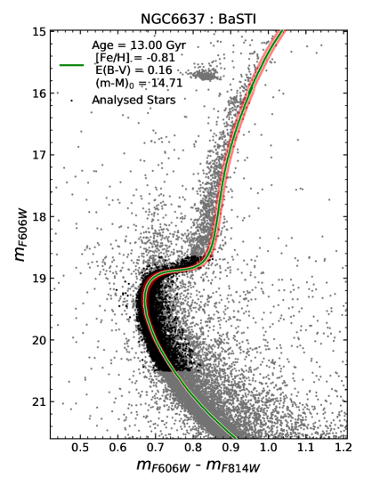
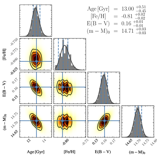
Figure 7: Results of the isochrone fits for NGC 6637 (M69) with BaSTI isochrones. (Left:) CMD with the isochrone representing the parameters of the central solution (green line). The black dots represent the stars used in the isochrone fitting, whereas the red region highlight the $1\sigma$ deviation around the solution (Right:) Corner plots showing the probability distribution function in all the free parameters. The parameters of the solution are shown along with the uncertainties in the upper right.

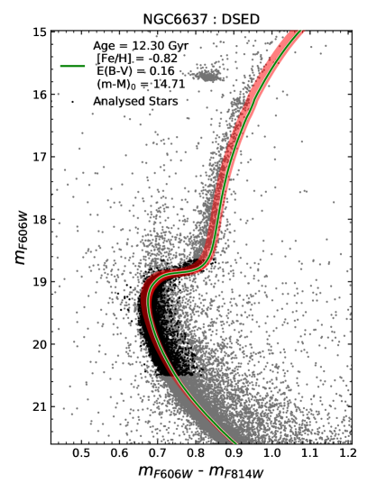
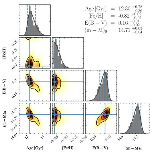
Figure 8: Same as Figure 7 for DSED isochrones.

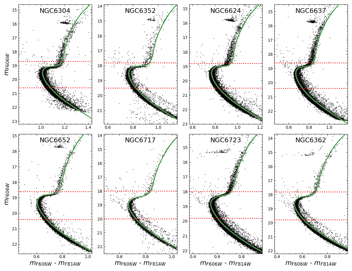
Figure 9: Results of the isochrone fits for all eight clusters with BaSTI isochrones. The red dotted lines represent the magnitude range adopted for the fitting.

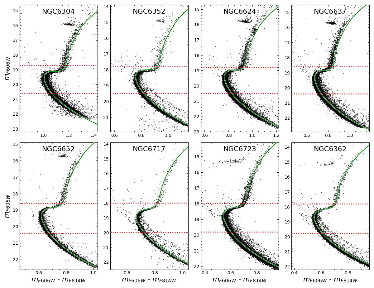
Figure 10: Same as Figure 9 for DSED isochrones.

4.1 Isochrone fitting: DSED and BaSTI

The results from the isochrone fitting considering each GC as a SSP and adopting two sets of isochrones (DSED and BaSTI) are shown in Table 4. The average result for each cluster is calculated as a simple average of the center values for BaSTI and DSED, and the non-symmetric uncertainties are calculated as the quadrature sum of the two model uncertainties.

The adopted free parameters are age, $\rm{[Fe/H]}$, $(m-M)_{0}$ and $E(B-V)$, but the apparent distance modulus $(m-M)_{V}$ and distance are also shown in Table 4. The ages and distance results are discussed in Section 4.2, and compared with previous literature results. The derived ages present a mean absolute error between $\sim 0.4$ and 0.8 Gyr, where the uncertainty propagation and the systematic errors from the comparison of DSED and BaSTI models are considered.

For the most metal-rich GCs, an important ingredient to be considered is the $\alpha$-enhancement. For NGC 6304 and NGC 6352 ($\rm{[Fe/H]}\sim-0.50$), we adopted $\rm{[\alpha/Fe]}=+0.2$, more consistent with the values from Table 2. The reason for this comes from the [$\alpha$/Fe] decrease with increasing metallicity (Barbuy et al., 2018a), such that it would correspond to $\rm{[\alpha/Fe]}\sim+0.2$ for these GCs. In this case, the isochrones were interpolated. Considering $\rm{[\alpha/Fe]}=+0.2$ leads to slightly older ages (relative to adopting $\rm{[\alpha/Fe]}=+0.4$). It suggests that other metal-rich clusters, where enhanced [$\alpha$/Fe] values were considered, may have to be reassessed (e.g. Lagioia et al., 2014). Further spectroscopic derivations of accurate $\alpha$-element abundances are greatly needed.

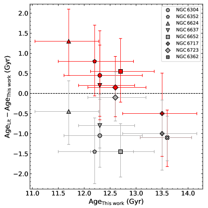
Figure 11: Comparison between the ages derived in Dotter et al. (2010, red symbols) and VandenBerg et al. (2013, gray symbols), and our derived ages. The result for NGC 6362 is the same in both literature works, then its symbol and the error bars overlap.

The best isochrone fits to CMDs and corresponding corner plots for NGC 6637 are presented in Figures 7 (BaSTI isochrones before the correction) and 8 (DSED isochrones). The best fit CMD can be seen in the central solution identified with the solid line, whereas the red area shows the region around the isochrone corresponding to the derived parameters within 1$\sigma$. The black dots correspond to the stars used in the isochrone fitting and the gray ones to all the observed stars. The corner plots present the probability distribution function derived for the free parameters in the diagonal panels and the correlations between two parameters in the other panels.

Figures 9 and 10 show the best isochrone fit to all the sample clusters, employing respectively the BaSTI and DSED isochrones. The fit is carried out to stars between the lower RGB and 1.0 magnitude below the MSTO, as shown by red dotted lines. RGB stars are avoided due to convection issues, as explained above, but even so the fits to the RGBs are very good in most cases.

4.2 Discussion on ages and distances

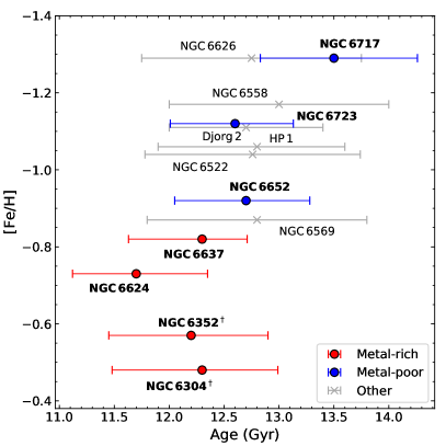
Figure 12: Distribution of the derived ages vs. metallicities in the range $-1.3<\rm{[Fe/H]}<-0.4$. The circles represent the seven sample bulge GCs (four moderately metal-rich in red and three moderately metal-poor in blue). The gray markers correspond to the other bulge GCs that have accurate age measurements in the literature: NGC 6626 and NGC 6522 (Kerber et al., 2018); NGC 6558 (Barbuy et al., 2018b); HP 1 (Kerber et al., 2019); NGC 6569 (Saracino et al., 2019); and Djorg 2 (Ortolani et al., 2019). Those marked with $\dagger$ correspond to $[\alpha\rm{/Fe}]=+0.2$.

Previous determinations of ages, distances and reddening values through isochrone fitting methods for the sample GCs are reported in Table 5, namely from: Dotter et al. (2010), VandenBerg et al. (2013) and O’Malley et al. (2017) adopting ACS photometry (F606W and F814W filters) from the GO-10775 program; Kerber et al. (2018) adopting ACS and WFC3 photometry (F625W and F438W filters) from GO-12008 and GO-13297 programs; and Saracino et al. (2016) with Gemini near-infrared data (GeMS+GSAOI).

Dotter et al. (2010) used an isochrone fitting method that consists in measuring the MSTO absolute magnitude and then interpolating an isochrone grid of the MSTO as a function of age and metallicity, with fixed $E(B-V)$ and absolute distance modulus $(m-M)_{0}$, applying DSED isochrones.

VandenBerg et al. (2013) derived the ages for 55 GCs from $\Delta_{\rm TO}^{\rm HB}$ measurement, with the Victoria-Regina models. They report that the ages derived for NGC 6304, NGC 6624 and NGC 6637 are the least reliable ones because their CMDs are strongly affected by differential reddening and field-star contamination.

Table 5: Literature ages, reddening and distance modulus derived for a given $\rm{[Fe/H]}$ and $\rm{[\alpha/Fe]}$.

Cluster	[Fe/H]	[$\alpha$/Fe]	$Y$	Age (Gyr)	$E(B-V)$	$d_{\odot}$ (kpc)	Model	Ref.
NGC 6304	$-0.50$	$+0.20$	0.25	$12.75\pm 0.75$	$0.482$	$6.21$	DSED	D10
	$-0.37$	$+0.22$	0.264	$11.25\pm 0.38$	$0.500$	$6.28$	V-R	VdB13
NGC 6352	$-0.80$	$+0.40$	0.25	$13.00\pm 0.50$	$0.258$	$5.29$	DSED	D10
	$-0.62$	$+0.37$	0.259	$10.75\pm 0.38$	$0.27$	$5.44$	V-R	VdB13
NGC 6624	$-0.50$	$+0.00$	0.25	$13.00\pm 0.55$	$0.258$	$8.19$	DSED	D10
	$-0.42$	$+0.25$	0.263	$11.25\pm 0.50$	$0.268$	$7.99$	V-R	VdB13
	$-0.60$	$+0.40$	$\sim 0.26$	$12.50\pm 0.50$	$0.28$	$7.91$	DSED, BaSTI, V-R	S16
NGC 6637	$-0.70$	$+0.20$	0.25	$12.50\pm 0.75$	$0.166$	$8.86$	DSED	D10
	$-0.59$	$+0.35$	0.260	$11.00\pm 0.38$	$0.163$	$8.97$	V-R	VdB13
NGC 6652	$-0.75$	$+0.20$	0.25	$13.25\pm 0.50$	$0.115$	$9.26$	DSED	D10
	$-0.76$	$+0.46$	0.257	$11.25\pm 0.25$	$0.116$	$9.59$	V-R	VdB13
	$-0.76$	$+0.40$	—	$11.4\pm 2.0$	$0.11$	$9.68$	DSED	OM17
NGC 6717	$-1.10$	$+0.20$	0.25	$13.00\pm 0.75$	$0.207$	$7.55$	DSED	D10
	$-1.26$	$+0.46$	0.250	$12.50\pm 0.50$	$0.225$	$7.27$	V-R	VdB13
NGC 6723	$-1.00$	$+0.20$	0.25	$12.75\pm 0.50$	$0.074$	$8.06$	DSED	D10
	$-1.10$	$+0.46$	0.250	$12.50\pm 0.25$	$0.07$	$8.05$	V-R	VdB13
	$-1.10$	$+0.40$	—	$11.9\pm 2.0$	$0.05$	$8.75$	DSED	OM17
NGC 6362	$-1.10$	$+0.40$	0.25	$12.50\pm 0.50$	$0.071$	$7.64$	DSED	D10
	$-1.07$	$+0.46$	0.25	$12.50\pm 0.25$	$0.076$	$7.46$	V-R	VdB13
	$-1.07$	$+0.40$	—	$11.4\pm 2.0$	$0.07$	$8.09$	DSED	OM17
	$-1.08$	$+0.40$	0.25	$13.7\pm 1.0$	$0.053$	$7.69$	DSED, BaSTI	K18

Note. — D10: Dotter et al. (2010); VdB13: VandenBerg et al. (2013, where V-R refers to the Victoria-Regina models); S16: Saracino et al. (2016); OM17: O’Malley et al. (2017); and K18: Kerber et al. (2018). The color excess $E(m_{\rm{F606W}}-m_{\rm{F814W}})$ and apparent distance moduli were transformed using the extinction coefficients from the PARSEC database and the transformation given in Campos et al. (2013).

Saracino et al. (2016) and Kerber et al. (2018) applied $\chi^{2}$ calculation in the isochrone fitting for NGC 6624 and NGC 6362 respectively. Saracino et al. (2016) kept the age as the only free parameter and assumed the minimum value of $\chi^{2}$ as the solution. On the other hand, Kerber et al. (2018) considered the age, distance modulus and reddening as the free parameters and also applied the emcee code to sample their posterior probabilities. O’Malley et al. (2017) applied a Monte Carlo analysis to carry out a MS-fitting to derive the ages and distances for 22 GCs, resulting in higher uncertainties.

Figure 11 compares the ages from Dotter et al. (2010, red symbols) and VandenBerg et al. (2013, gray symbols) with our results (Table 4). In general, the results from Dotter et al. (2010) are around 0.5 Gyr older than our results, whereas those from VandenBerg et al. (2013) point systematically toward $1.0-1.5$ Gyr younger ages, showing a disagreement larger than the error bars. Most of the Dotter et al. (2010) derived ages are compatible within 1$\sigma$ with the present results.

Figure 12 shows the distribution of derived ages vs. metallicities, updating an interesting plot presented in Saracino et al. (2019, their Figure 16). The moderately metal-poor GCs ($\rm{[Fe/H]}\lesssim-0.85$) appear to be slightly older than the metal-rich ones, with average ages of $12.86\pm 0.36$ Gyr and $12.12\pm 0.32$ Gyr respectively. The very low statistics of objects, the individual age uncertainties of $\sim 0.50$ Gyr and the probability that several of the metal-rich ones might be assigned to a thick disk population, (Pérez-Villegas et al., 2020), prevent any further conclusion on systematic age difference as a function of $\rm{[Fe/H]}$ for bulge clusters. It is worth noting that some clusters analyzed here (NGC 6717 and NGC 6362) and in previous works (e.g. Kerber et al., 2018, 2019) are revealed to be among the oldest GCs in the Galaxy.

For all clusters the ages from DSED and BaSTI are compatible within 1$\sigma$. The clusters NGC 6304 and NGC 6624 show the largest age differences between the derivations based on DSED and BaSTI, amounting to 1.3 Gyr and 0.7 Gyr respectively. This is due to their larger reddening, and consequently a larger uncertainty in the distances – see discussion in Pérez-Villegas et al. (2020). As a matter of fact, the uncertainty in distances is a major difficulty for establishing precise ages and orbits.

The derived metallicities are in very good agreement within 1$\sigma$ with the adopted values in the Gaussian priors (Table 3). For the GCs that presented at least one member RRL (NGC 6717, NGC 6723 and NGC 6362), the derived apparent distance moduli $(m-M)_{V}$ are also compatible with those given by RRL mean magnitudes (Figure 6). The derived distances and reddening values (Table 4) are also consistent with those from Dotter et al. (2010), VandenBerg et al. (2013), Saracino et al. (2016) and Kerber et al. (2018), as shown in Table 5.

Comparing our derived distances with those obtained from the Gaia DR2 parallaxes (Gaia Collaboration et al., 2018b), given in Pérez-Villegas et al. (2020) for bulge GCs, a rather large discrepancy from $20$ to $65$ per cent is observed for NGC 6304, NGC 6352, NGC 6637 and NGC 6723. For NGC 6624, NGC 6652 and NGC 6717, this discrepancy remains below $10\%$. For these large distances the Gaia DR2 parallaxes are often not suitable (see Pérez-Villegas et al., 2020).

5 Multiple Stellar Population Analysis

In Milone et al. (2017, Paper IX), the identification of the multiple stellar populations, with the “chromosome map” diagram, was described in detail and applied to the RGB stars for the 56 GCs from the GO-13297 program. Previously, Milone et al. (2015, Paper III) performed the identification of the MPs in both the MS and RGB of NGC 2808, also using this diagram.

In this work, we distinguish the MPs from the MS to the RGB, including the SGB, to carry out the isochrone fitting both to the first (1G) and second generation (2G) stars simultaneously, and to check whether there occurs any detectable age difference.

Note that, in the pseudo-color $C_{\rm F275W,F336W,F438W}=(m_{\rm F275W}-m_{\rm F336W})-(m_{\rm F336W}-m_{\rm F438W})$, F275W, F336W, and F438W are dominated by OH, NH and CN bands respectively. C, O are anticorrelated with respect to N in 2G stars. In particular, a 2G star is fainter than 1G stars in F336W because it is N and Na-richer, and brighter than 1G stars in F275W and F438W filters because they are O- and C-poorer, compared to 1G stars. The filter F336W is counted twice in the pseudo-color, thus enhancing the contrast (Paper I).

In some combinations of colors and magnitudes in different CMDs, the MPs seem to be entangled in the SGB region, as they are not horizontally separated from each other (Section 5.2). The chromosome map basically rectifies a distribution of stars, and shows whether it follows a bimodal (or multimodal) horizontal distribution. Therefore, it cannot be applied to SGB stars, since this region is typically horizontal in CMDs.

5.1 Stellar population separation in RGB and MS: Chromosome maps

The original chromosome map analysis was presented in Paper IX. Here we apply the same method, but improved in terms of a more accurate separation of MPs. This is obtained by applying GMM algorithms (for details see Souza et al., 2020). We also compute the fractions of stars from first (N₁/N_TOT) and second generations and compare our results to those from Paper IX in Table 6, showing a good agreement.

Paper IX concluded that the seven GCs of the present sample are type-I clusters, meaning that their chromosome maps do not present additional sequences and that their 1G and 2G stars can be separated more clearly for some clusters such as NGC 6352, and less so for cases as NGC 6304. These patterns are also observed in the present analysis, where we use an automatic approach allowing to separate satisfactorily the MPs, even for NGC 6304 (Figure 13).

Table 6: Comparison between the fractions of 1G stars over the total number of RGB stars from Milone et al. (2017, M17) and the values derived in the present work.

Cluster	($N_{1}$/$N_{\rm TOT}$)M17	$N_{1}$/$N_{\rm TOT}$
NGC 6304	—	$0.362\pm 0.059$
NGC 6352	$0.474\pm 0.035$	$0.426\pm 0.041$
NGC 6624	$0.279\pm 0.020$	$0.462\pm 0.103$
NGC 6637	$0.425\pm 0.017$	$0.481\pm 0.036$
NGC 6652	$0.344\pm 0.026$	$0.371\pm 0.041$
NGC 6717	$0.637\pm 0.039$	$0.635\pm 0.052$
NGC 6723	$0.363\pm 0.017$	$0.377\pm 0.029$
NGC 6362	$0.574\pm 0.035$	$0.584\pm 0.041$

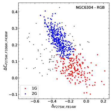
Figure 13: Chromosome map of RGB stars in NGC 6304. The 1G and 2G were separated using GMM techniques.

Note that the fraction of 1G stars for NGC 6717 ([Fe/H] $=-1.26$) is 0.635, which is among the three largest 1G fractions presented in Paper IX, together with NGC 6101 and NGC 6496. The chromosome maps applied to the RGB (top panel) and MS (bottom panel) stars of NGC 6637 are presented in Figure 14. For the MS stars, where the chromosome map is much more populated, we have excluded from the analysis the stars (grey points) outside the $3\sigma$ level of the fitted Gaussian models.

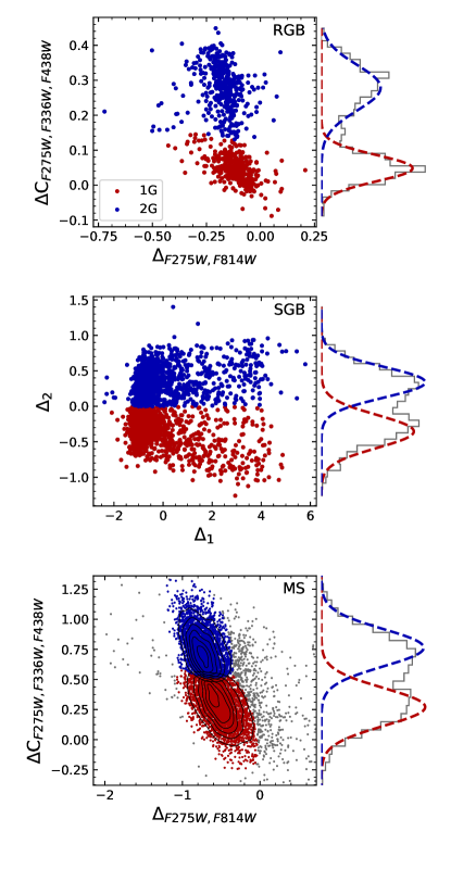
Figure 14: Chromosome maps with the derived Gaussian distributions showing the MPs separation for NGC 6637, considering the RGB (top panel), MS (bottom panel), and the two-color diagram applied to SGB (middle panel) stars. In the middle panel, $\Delta_{1}$ and $\Delta_{2}$ are the coordinates obtained by rotating the original two-color diagram counterclockwise by an angle $\theta=45^{\circ}$. Since the MS is much more populated, we overplot the contour lines relative to the two stellar generations.

5.2 Stellar population separation in the SGB: Two-color diagrams

The SGB morphology is a function of metallicity and of the choice of magnitude in the CMD. In general terms, the chromosome map is not effective to separate the stellar generations among these stars. Here, we apply the conventional two-color diagram $m_{\rm F336W}-m_{\rm F438W}$ vs. $m_{\rm F275W}-m_{\rm F336W}$, as described in Nardiello et al. (2015, Paper IV), with the implementation of the GMM algorithm (Souza et al., 2020).

The result for the SGB stars of NGC 6637 is presented in the middle panel of Figure 14 with a counterclockwise rotation of $45^{\circ}$, showing an evident separation of the MPs in the horizontal direction and a clear bimodality in the histogram.

Gathering the results from the MS to the RGB, several combinations of CMDs can be tested. An example is shown in Figure 15 (similar to Figure 2 from Paper I), where the panels have the same magnitude $m_{\rm F336W}$, but adopting colors such that the pseudo-color (left panel) is defined by the subtraction of the two subsequent colors. As shown in Paper I, the 2G stars (N-rich and C-poor) are bluer in the color $m_{\rm F275W}-m_{\rm F336W}$ than the 1G stars, but redder in $m_{\rm F336W}-m_{\rm F438W}$. This is the reason why $C_{\rm F275,F336W,F438W}$ maximizes the MP separation, combining the “magic trio” of WFC3 filters.

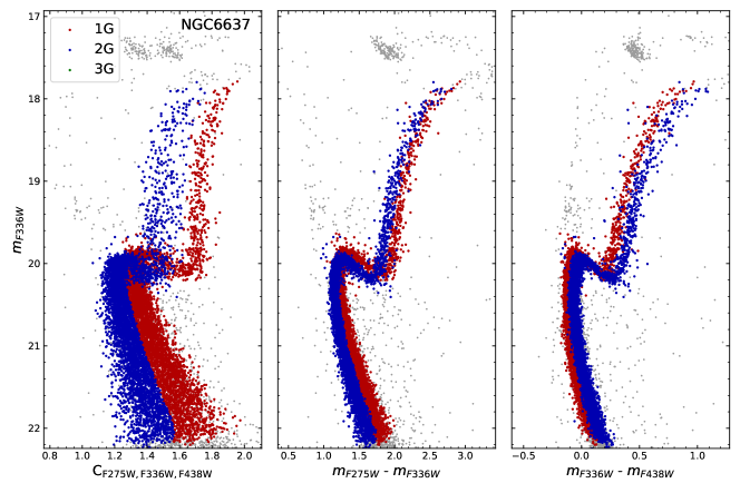
Figure 15: MS-to-RGB MPs separation in CMD of NGC 6637, from UV magnitudes, colors, and pseudo-colors.

5.3 Multiple stellar populations: age differences

Derivations of age differences between stellar generations in a cluster were carried out previously by Milone et al. (2008) and Cassisi et al. (2008) for NGC 1851; Roh et al. (2011) for NGC 288; Marino et al. (2012a) and Villanova et al. (2014) for $\omega$ Cen; Marino et al. (2012b) for NGC 6656; Joo & Lee (2013) for $\omega$ Cen, M22 and NGC 1851; Lee et al. (2013) for NGC 2419; and Souza et al. (2020) for NGC 6752. In this collaboration, Nardiello et al. (2015, Paper IV) obtained age differences for NGC 6352, applying $\chi^{2}$ calculations for the isochrone fitting over synthetic CMDs. They infer a helium abundance variation of $\Delta Y=0.029\pm 0.006$, and estimate an age difference of $10\pm 110$ Myr assuming no difference in $\rm{[Fe/H]}$ and $\rm{[\alpha/Fe]}$, with this uncertainty rising to $\sim 300$ Myr if a difference of 0.02 is considered in both.

In this work, the age derivation was achieved from the 1G and 2G ($m_{\rm F606W}$ vs. $m_{\rm F606W}-m_{\rm F814W}$) CMDs simultaneously. The analysis was carried out first considering the canonical helium for both populations. As described in Souza et al. (2020), the likelihood function for MPs assumes that the two stellar populations have the same distributions of $E(B-V)$ and $(m-M)_{0}$ to perform the isochrone fitting, whereas [Fe/H] is fixed. In that way, the best fit represents the best result for 1G and 2G at the same time. After that, both generations are fitted assuming for 2G the values of helium enhancement derived by Milone et al. (2018b, Paper XVI).

We derive a weighted mean age difference ($\left\langle\delta\tau_{\rm{1G,2G}}\right\rangle$) of $41\pm 170$ Myr, for the eight sample clusters considering the canonical helium for both populations, as shown in Table 7. This value reduces to $17\pm 170$ Myr when the helium enhancement is taken into account. Recalling that the individual age differences present an uncertainty of $\sim 500$ Myr, these smaller uncertainties were obtained by weighting the uncertainties of the eight individual measurements. Figure 16 shows the isochrone fitting for the MPs of NGC 6637. In the case of canonical He for 2G stars (top panels), a negative age difference was derived for this cluster. The derived age difference vanishes with the He enhancement in 2G (bottom panels), and shows a better fit for 2G stars.

It is interesting to compare the age difference obtained for NGC 6352, with the results by Nardiello et al. (2015). We adopted $\rm{[Fe/H]}=-0.59$, $[\alpha\rm{/Fe]}=+0.2$, canonical He abundance and $\Delta$Y = 0.027 for the 2G. Nardiello et al. (2015) adopted $\rm{[Fe/H]}=-0.67$, $[\alpha\rm{/Fe]}=+0.4$, He abundance and $\Delta$Y = 0.029 for the 2G. An age difference of $10\pm 110$ Myr was derived by Nardiello et al. (2015), which is compatible within errors with the age difference derived by us, of $500\pm 480$ Myr.

Table 7: Age differences derived for the MPs, adopting both primordial and enhanced helium abundances.

Cluster	$\delta Y_{\rm max}$	$\delta\tau_{\rm 1G,2G}$	$\delta\tau_{\rm 1G,2G}^{\dagger}$
		(Gyr)	(Gyr)
NGC 6304‡	$0.025\pm 0.006$	$-0.10^{+0.42}_{-0.46}$	$-0.10^{+0.49}_{-0.45}$
NGC 6352‡	$0.027\pm 0.006$	$0.40^{+0.49}_{-0.48}$	$0.50^{+0.47}_{-0.48}$
NGC 6624	$0.023\pm 0.003$	$-0.10^{+0.46}_{-0.45}$	$0.00^{+0.43}_{-0.50}$
NGC 6637	$0.012\pm 0.005$	$-0.20^{+0.58}_{-0.41}$	$0.00^{+0.41}_{-0.36}$
NGC 6652	$0.017\pm 0.011$	$-0.10^{+0.53}_{-0.41}$	$0.00^{+0.55}_{-0.49}$
NGC 6717	$0.003\pm 0.009$	$0.70^{+0.68}_{-0.70}$	$0.30^{+0.70}_{-0.72}$
NGC 6723	$0.025\pm 0.007$	$0.00^{+0.51}_{-0.39}$	$-0.10^{+0.51}_{-0.39}$
NGC 6362	$0.004\pm 0.011$	$0.10^{+0.44}_{-0.42}$	$-0.20^{+0.40}_{-0.41}$

Note. — ^† Results with helium enhancement in 2G stars, according with Paper XVI. ^‡ $\rm{[\alpha/Fe]}=+0.2$.

Systematic uncertainties in low-mass stellar models, affecting the cluster age dating process, are mainly dominated by the treatment of superadiabatic convection, diffusive process efficiency and low-temperature opacity; to these sources of uncertainty one has to also add the error associated with the still-present shortcomings in the bolometric corrections and effective temperature - color relations. To firmly assess how much these systematics contribute in the error budget of the GC age determination is difficult because it depends on the metallicity range and adopted photometric systems. Data listed in Table 4 show that two independent, recent sets of isochrones predict GC ages with a difference ranging between 0.1 and 1.0 Gyr; when also accounting for the errors in the photometry and binary star contamination in the MSTO region, it is safe to assume a realistic error on the derived age of $\sim 0.5-0.8$ Gyr.

In the case of relative ages such as the comparison between 1G and 2G, most of these error sources are cancelled (all the zero points both of the photometry and the models), but an additional source is added due to the effects of the individual element abundance variation, in particular C, N, O and He. It is well known that the helium, carbon, nitrogen and oxygen play an important role. The chemical abundance uncertainties have an effect on the models and on the opacities. In conclusion, a conservative uncertainty of $\pm$0.5 Gyr in the ages can be adopted, and therefore, although the 2G generation is, as expected, younger than 1G, the age difference between 1G and 2G are within errors, and the quantitative difference cannot be specified.

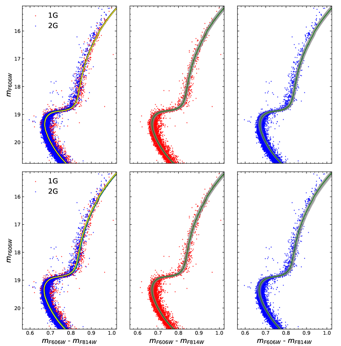
Figure 16: Isochrone fitting of MPs for NGC 6637, considering canonical helium for both stellar populations (top panels), and considering helium enhancement for 2G stars (bottom panels). The dark region represents the result within 3$\sigma$.

6 Conclusions

The primary aim of the HST UV Legacy Survey of Galactic GCs collaboration was the identification of multiple stellar populations in globular clusters. In Milone et al. (2017, Paper IX) and Milone et al. (2015, Paper III), a method of stellar population separation was applied to the RGB and MS of the sample clusters. Milone et al. (2012b) and Nardiello et al. (2015, Paper IV) analyzed the SGB stars based on two-color diagrams. We applied the methods described in the above cited papers to separate the stellar populations from the MS to the RGB, with the fraction of 1G and 2G stars given in Table 6.

In the present work we derive ages for the seven bulge globular clusters included in Piotto et al. (2015), both for a single stellar population as well as for the first and second stellar generations. For the derivation of age, distance, and reddening, we employed our new code SIRIUS (Souza et al., 2020), that uses Markov chain Monte Carlo algorithm for the fitting of the isochrones to the observed CMDs. The $\alpha$-enhanced Dartmouth and BaSTI isochrones were used for all clusters, for the analysis of single stellar populations (Table 4).

As shown in Figure 12 (updated from Saracino et al., 2019), we derived a weighted average age of $12.86\pm 0.36$ Gyr and $12.12\pm 0.32$ Gyr for the moderately metal-poor and for the more metal-rich bulge clusters respectively. We cannot conclude that this corresponds to systematic age difference as a function of $\rm{[Fe/H]}$ among bulge clusters, due to a low statistics of objects, the individual age uncertainties of 500 Myr, and moreover, given that 3 of the metal-rich clusters appear to belong to a thick disk (and not bulge) population. The clusters NGC 6717 and NGC 6362 (the latter being a reference halo cluster) are revealed to be among the oldest MW clusters with $\sim 13.5$ Gyr (Kerber et al., 2018, 2019). Adopting lower $\rm{[\alpha/Fe]}$ values for the more metal-rich GCs can influence their ages, as applied here for NGC 6304 and NGC 6352, and further detailed studies using original (not interpolated) sets of isochrones are needed. Also, accurate $\alpha$-element abundances from high-resolution spectroscopy are of great interest for further improving the precision in the age derivation.

We also derived age differences between 1G and 2G populations. A weighted mean difference produced by our statistical fitting procedure, results to be of $41\pm 170$ Myr adopting canonical He for both and smaller for enhanced helium, reaching $17\pm 170$ Myr. For each individual cluster, the typical uncertainty of the age difference between 1G and 2G is around $500$ Myr (Table 7), being of the same order as the assumed error on ages of $\pm$0.5 Gyr.

In the derivation of relative ages of 1G and 2G stellar populations, most of the sources of errors on absolute ages are cancelled (zero points in the photometry and the models), but the effects of the element abundance variations in C, N, O and in particular in He are added instead. Therefore, adopting a conservative uncertainty of $\pm$0.5 Gyr in the individual age differences, these quantitative values cannot be used to constrain models on the formation of 2G stars (see Renzini et al., 2015; D’Antona et al., 2016; Bastian & Lardo, 2018).

Models for the formation of multiple populations predict age differences between first and second generations, from about zero up to 150 Myr (Gieles et al., 2018; Decressin et al., 2007; D’Ercole et al., 2008; D’Antona et al., 2016; Milone et al., 2017). An uncertainty of 0.5 Gyr is typical for the age of each individual cluster, whereas the weighted uncertainty from the eight studied clusters results to be of $0.17$ Gyr. Within these uncertainties in the present age derivations, we cannot discriminate between the different formation scenarios. This is due to the intrinsic uncertainties inherent to detailed physics processes taken into account in stellar evolution models.

The present results add to the previous literature regarding the age of the moderately metal-poor bulge globular clusters. This has an impact on the epoch of bulge and globular cluster formation (e. g. Barbuy et al., 2018a). The verification that the bulge clusters are older than 11 Gyr is an important information with respect to the time of bar formation. According to Buck et al. (2018), from cosmological simulations, the bar should have formed at about $8\pm 2$ Gyr ago. Also Bovy et al. (2019) estimated that the Galactic bar formed $\sim 8$ Gyr ago, from an analysis of chemical abundances of field stars, from the Apache Point Observatory Galactic Evolution Experiment (APOGEE) survey, combined with kinematical information from the Gaia collaboration. From this age difference, we can conclude that the globular clusters were formed early in the Galaxy, before the bar formation, and were later trapped by the bar (see also Renzini et al., 2018). Therefore, scenarios of bar/bulge formation have to take into account the old ages of the bulge globular clusters. It would be interesting to extend the analysis to the other clusters of the UV Legacy Survey of Globular Clusters.

Appendix A Literature information on the sample clusters

This appendix contains a bibliographic review on the sample GCs, regarding the photometry and age derivations by isochrone fitting. We follow here the examples and references given in Alonso-García et al. (2012) and Roediger et al. (2014).

A.1 NGC 6304

Ortolani et al. (2000) obtained B and V photometry of NGC 6304 and derived $E(B-V)\approx 0.5$, $d_{\odot}\approx 6$ kpc and [Fe/H] $\approx-0.6$, and provides a review of previous results. Valenti et al. (2005) observed this GC and NGC 6637 in the JHK filters from ESO/NTT telescope, and estimated $\rm{[Fe/H]}=-0.70$, $E(B-V)=0.58$ and absolute distance modulus of $(m-M)_{0}=13.88$, i.e. a distance of $\sim 6.0$ kpc.

NGC 6304 contains X-ray sources, and has been extensively observed in the study of quiescent low-mass X-ray binaries and radio pulsars (Guillot et al., 2009, 2013, and references therein).

A.2 NGC 6352

This cluster has several photometric studies on the literature. The most recent is Pulone et al. (2003), with the F606W and F814W HST filters (WFPC2), estimating an age of 14 Gyr, a distance modulus of $(m-M)_{0}=13.6$ and $E(B-V)=0.25$. Faria & Feltzing (2002) analyzed older HST data in the F555W and F814W filters, and derived an age of 12.6 Gyr, $(m-M)_{0}=13.58$ and $E(B-V)=0.26$. They also compared this cluster with NGC 6624 and NGC 6637 (studied by Heasley et al., 2000), presenting similar ages and metallicities. Previous photometry from ground-based (Rosenberg et al., 2000; Sarajedini & Norris, 1994) and space-based (Fullton et al., 1995) telescopes were obtained, but no precise age derivation was carried out.

Pancino et al. (2010) first showed the presence of MPs in this outer bulge/disk cluster, detecting a bimodal CN and CH anticorrelation analyzing low-resolution spectra of MS stars. Feltzing et al. (2009) derived the metallicity ($\rm{[Fe/H]}=-0.55\pm 0.03$) and abundances for $\alpha$- and iron-peak elements, from high-resolution UVES/VLT spectra of HB stars, as reported in Table 2. Previously, Gratton (1987) derived $\rm{[Fe/H]}=-0.79\pm 0.06$ and the other abundances, but we adopted the Feltzing et al. (2009) results in the prior.

Inside this HST collaboration, two works were focused on the NGC 6352 MPs: Nardiello et al. (2015, Paper IV) study the age and helium differences between them, and Libralato et al. (2019, Paper XVIII) analyze their radial distribution and kinematics.

A.3 NGC 6624

Heasley et al. (2000) present the $V$ vs. $V-I$ observed CMD based on WFPC2/HST photometry, deriving an apparent distance modulus of $(m-M)_{V}=15.42$ and $E(V-I)=0.42$. Valenti et al. (2011) obtained infrared spectra for 5 stars with NIRSPEC at Keck II, deriving a metallicity [Fe/H] $=-0.69$ and abundance ratios as shown in Table 2, with a mean $\alpha$-element enhancement of [$\alpha$/Fe] $=+0.39$. They also determine a radial velocity of $-$47 km s^-1.

This cluster hosts the low-mass X-ray binary 4U/1820-30, source of X-rays and gamma-rays, that is extensively observed (Peuten et al., 2014). It also contains 6 millisecond pulsars (Biggs et al., 1994; Lynch et al., 2012).

A.4 NGC 6637 (M69)

Heasley et al. (2000) derive an apparent distance modulus $(m-M)_{V}=15.29$ and reddening $E(V-I)=0.24$ from WFPC2/HST data for NGC 6637. Valenti et al. (2005) obtained near-infrared photometry with SOFI@NTT/ESO, deriving a metallicity [Fe/H] $=-0.68$, $E(B-V)=0.14$ and $(m-M)_{0}=14.87$, i.e. an heliocentric distance of $d_{\odot}=9.42$ kpc.

A.5 NGC 6652

Ortolani et al. (1994) obtained CMDs in BVRIz, and estimated a metallicity of $\rm{[Fe/H]}=-0.9$, and a distance to the Sun of d_⊙ = 9.3 kpc. From HST CMDs in filters F555W and F814W, Chaboyer et al. (2000) obtained a distance to the Galactic center of $R_{\rm GC}=2$ kpc, and $\rm{[Fe/H]}=-0.85$. This cluster has several X-ray binaries, and pulsars (Stacey et al., 2012; DeCesar et al., 2015, and references therein).

A.6 NGC 6717 (Palomar 9)

Brocato et al. (1996) observed the first deep $V$ vs. $B-V$ CMD for this cluster, identifying a moderately blue extended HB and estimated $E(B-V)=0.22$ and $\rm{[Fe/H]}=-1.26\pm 0.10$. Ortolani et al. (1999) obtained B,V CMDs, deriving $E(B-V)=0.23$, and a distance of d${}_{\odot}=7.1$ kpc, placing the cluster in the outskirts of the Galactic bulge. A metallicity of $\rm{[Fe/H]}\sim-1.3$ was estimated, and a blue horizontal branch was also identified. Goranskii (1979) identified the only catalogued RR Lyrae in the cluster field so far, obtaining $V=15.7$, which was used in the present RR Lyrae analysis (Figure 5). X-ray sources were recently detected in this cluster (Morris & Mitchel, 2015).

A.7 NGC 6723

Alcaíno et al. (1999) obtained CCD CMDs in B, V, I, and deduced $E(B-V)=0.11$, and estimated a metallicity of $\rm{[Fe/H]}=-1.22$. Gratton et al. (2015) obtained a metallicity of $\rm{[Fe/H]}=-1.22$, and derived abundances of O, N, Na, Mg, Ca, Ni, and Ba. These authors studied in detail the Na-O anticorrelation, indicative of a second generation stellar population, and were able to identify their location in the horizontal branch. Rojas-Arriagada et al. (2016) carried out a detailed abundance analysis of 7 red giants, yielding $\rm{[Fe/H]}=-0.98$, and radial velocity of $-96\pm 3.6$ km.s^-1. Abundances of O, Mg, Si, Ca, Ti, Na, Al and Ba are reported in Table 2.

It is interesting to note that NGC 6717 and NGC 6723 are similar to other bulge clusters with blue HBs: HP 1, NGC 6522, NGC 6558, AL 3, Terzan 10 within the inner $6^{\circ}$, and NGC 6325, NGC 6355, NGC 6453, NGC 6626, NGC 6642 in the outer bulge within $12^{\circ}$ of the Galactic center.

A.8 NGC 6362

NGC 6362 is an inner halo globular cluster, located at $\ell=-34.45^{\circ}$ and $b=-17.57^{\circ}$, with a reddening of $E(B-V)=0.11$. High-resolution abundance analyses by Mucciarelli et al. (2016) and Massari et al. (2017) indicate metallicity values of $\rm{[Fe/H]}=-1.09\pm 0.01$ and $\rm{[Fe/H]}=-1.07\pm 0.01$, respectively. Mucciarelli et al. (2016) found evidence of multiple stellar populations, through a Na-O anticorrelation, and suggest that this is the lowest mass globular cluster with multiple populations. The age of NGC 6362 has been extensively analyzed in the literature, e.g. De Angeli et al. (2005), Meissner & Weiss (2006), Marín-Franch et al. (2009), Dotter et al. (2010), Paust et al. (2010), VandenBerg et al. (2013), Wagner-Kaiser et al. (2017) and Kerber et al. (2018). The latter authors deduce an age of $\sim 13$ Gyr for this cluster.

References

- Alcaíno et al. (1999) Alcaíno, G., Liller, W., Alvarado, F., et al. 1999, A&AS, 136, 461
- Alonso-García et al. (2012) Alonso-García, J., Mateo, M., Sen, B., et al. 2012, AJ, 143, 70
- Anderson et al. (2008) Anderson, J., Sarajedini, A., Bedin, L. R., et al. 2008, AJ, 135, 2055
- Barbuy et al. (2018a) Barbuy, B., Chiappini, C., & Gerhard, O. 2018a, ARA&A, 56, 223
- Barbuy et al. (2018b) Barbuy, B., Muniz, L., Ortolani, S., et al. 2018b, A&A, 619, A178
- Bastian & Lardo (2018) Bastian, N., & Lardo, C. 2018, ARA&A, 56, 83
- Baumgardt & Hilker (2018) Baumgardt, H., & Hilker, M. 2018, MNRAS, 478, 1520
- Bedin et al. (2005) Bedin, L. R., Cassisi, S., Castelli, F., et al. 2005, MNRAS, 357, 1038
- Bedin et al. (2004) Bedin, L. R., Piotto, G., Anderson, J., et al. 2004, ApJ, 605, L125
- Bellini et al. (2009) Bellini, A., Piotto, G., Bedin, L. R., et al. 2009, A&A, 493, 959
- Bellini et al. (2013) Bellini, A., Piotto, G., Milone, A. P., et al. 2013, ApJ, 765, 32
- Bica et al. (2016) Bica, E., Ortolani, S., & Barbuy, B. 2016, PASA, 33, e028
- Biggs et al. (1994) Biggs, J. D., Bailes, M., Lyne, A. G., Goss, W. M., & Fruchter, A. S. 1994, MNRAS, 267, 125
- Bovy et al. (2019) Bovy, J., Leung, H. W., Hunt, J. A. S., et al. 2019, MNRAS, 490, 4740
- Bressan et al. (2012) Bressan, A., Marigo, P., Girardi, L., et al. 2012, MNRAS, 427, 127
- Brocato et al. (1996) Brocato, E., Buonanno, R., Malakhova, Y., & Piersimoni, A. M. 1996, A&A, 311, 778
- Brown et al. (2016) Brown, T. M., Cassisi, S., D’Antona, F., et al. 2016, ApJ, 822, 44 (Paper VII)
- Buck et al. (2018) Buck, T., Ness, M. K., Macciò, A. V., Obreja, A., & Dutton, A. A. 2018, ApJ, 861, 88
- Busso et al. (2007) Busso, G., Cassisi, S., Piotto, G., et al. 2007, A&A, 474, 105
- Campos et al. (2013) Campos, F., Kepler, S. O., Bonatto, C., & Ducati, J. R. 2013, MNRAS, 433, 243
- Carretta et al. (2009) Carretta, E., Bragaglia, A., Gratton, R., D’Orazi, V., & Lucatello, S. 2009, A&A, 508, 695
- Cassisi et al. (2013) Cassisi, S., Mucciarelli, A., Pietrinferni, A., Salaris, M., & Ferguson, J. 2013, A&A, 554, A19
- Cassisi et al. (2008) Cassisi, S., Salaris, M., Pietrinferni, A., et al. 2008, ApJ, 672, L115
- Chaboyer et al. (2000) Chaboyer, B., Sarajedini, A., & Armandroff, T. E. 2000, AJ, 120, 3102
- Clement et al. (2001) Clement, C. M., Muzzin, A., Dufton, Q., et al. 2001, AJ, 122, 2587
- Clementini et al. (2003) Clementini, G., Gratton, R., Bragaglia, A., et al. 2003, AJ, 125, 1309
- Cohen et al. (2018) Cohen, R. E., Mauro, F., Alonso-García, J., et al. 2018, AJ, 156, 41
- Cohen et al. (2014) Cohen, R. E., Mauro, F., Geisler, D., et al. 2014, AJ, 148, 18
- Conroy et al. (2018) Conroy, C., Villaume, A., van Dokkum, P. G., & Lind, K. 2018, ApJ, 854, 139
- Correnti et al. (2016) Correnti, M., Gennaro, M., Kalirai, J. S., Brown, T. M., & Calamida, A. 2016, ApJ, 823, 18
- Correnti et al. (2018) Correnti, M., Gennaro, M., Kalirai, J. S., Cohen, R. E., & Brown, T. M. 2018, ApJ, 864, 147
- Crestani et al. (2019) Crestani, J., Alves-Brito, A., Bono, G., Puls, A. A., & Alonso-García, J. 2019, MNRAS, 1639
- Dambis et al. (2013) Dambis, A. K., Berdnikov, L. N., Kniazev, A. Y., et al. 2013, MNRAS, 435, 3206
- D’Antona et al. (2018) D’Antona, F., Caloi, V., & Tailo, M. 2018, Nature Astronomy, 2, 270
- D’Antona et al. (2017) D’Antona, F., Milone, A. P., Tailo, M., et al. 2017, Nature Astronomy, 1, 0186
- D’Antona et al. (2016) D’Antona, F., Vesperini, E., D’Ercole, A., et al. 2016, MNRAS, 458, 2122
- De Angeli et al. (2005) De Angeli, F., Piotto, G., Cassisi, S., et al. 2005, AJ, 130, 116
- DeCesar et al. (2015) DeCesar, M. E., Ransom, S. M., Kaplan, D. L., Ray, P. S., & Geller, A. M. 2015, ApJ, 807, L23
- Decressin et al. (2007) Decressin, T., Meynet, G., Charbonnel, C., Prantzos, N., & Ekström, S. 2007, A&A, 464, 1029
- D’Ercole et al. (2008) D’Ercole, A., Vesperini, E., D’Antona, F., McMillan, S. L. W., & Recchi, S. 2008, MNRAS, 391, 825
- Dias et al. (2016) Dias, B., Barbuy, B., Saviane, I., et al. 2016, A&A, 590, A9
- Dias et al. (2015) —. 2015, A&A, 573, A13
- Dotter et al. (2008) Dotter, A., Chaboyer, B., Jevremović, D., et al. 2008, ApJS, 178, 89
- Dotter et al. (2010) Dotter, A., Sarajedini, A., Anderson, J., et al. 2010, ApJ, 708, 698
- Faria & Feltzing (2002) Faria, D., & Feltzing, S. 2002, in Astronomical Society of the Pacific Conference Series, Vol. 274, Observed HR Diagrams and Stellar Evolution, ed. T. Lejeune & J. Fernandes, 373
- Feltzing et al. (2009) Feltzing, S., Primas, F., & Johnson, R. A. 2009, A&A, 493, 913
- Ferraro et al. (2016) Ferraro, F. R., Massari, D., Dalessandro, E., et al. 2016, ApJ, 828, 75
- Foreman-Mackey et al. (2013) Foreman-Mackey, D., Hogg, D. W., Lang, D., & Goodman, J. 2013, PASP, 125, 306
- Fullton et al. (1995) Fullton, L. K., Carney, B. W., Olszewski, E. W., et al. 1995, AJ, 110, 652
- Gaia Collaboration et al. (2016) Gaia Collaboration, Prusti, T., de Bruijne, J. H. J., et al. 2016, A&A, 595, A1
- Gaia Collaboration et al. (2017) Gaia Collaboration, Clementini, G., Eyer, L., et al. 2017, A&A, 605, A79
- Gaia Collaboration et al. (2018a) Gaia Collaboration, Brown, A. G. A., Vallenari, A., et al. 2018a, A&A, 616, A1
- Gaia Collaboration et al. (2018b) Gaia Collaboration, Helmi, A., van Leeuwen, F., et al. 2018b, A&A, 616, A12
- Gieles et al. (2018) Gieles, M., Charbonnel, C., Krause, M. G. H., et al. 2018, MNRAS, 478, 2461
- Goranskii (1979) Goranskii, V. P. 1979, Soviet Ast., 23, 510
- Gratton (1987) Gratton, R. C. 1987, A&A, 177, 177
- Gratton et al. (2012) Gratton, R. G., Carretta, E., & Bragaglia, A. 2012, A&A Rev., 20, 50
- Gratton et al. (2015) Gratton, R. G., Lucatello, S., Sollima, A., et al. 2015, A&A, 573, A92
- Guillot et al. (2009) Guillot, S., Rutledge, R. E., Brown, E. F., Pavlov, G. G., & Zavlin, V. E. 2009, ApJ, 699, 1418
- Guillot et al. (2013) Guillot, S., Servillat, M., Webb, N. A., & Rutledge, R. E. 2013, ApJ, 772, 7
- Harris (1996) Harris, W. E. 1996, AJ, 112, 1487
- Heasley et al. (2000) Heasley, J. N., Janes, K. A., Zinn, R., et al. 2000, AJ, 120, 879
- Hesser et al. (1977) Hesser, J. E., Hartwick, F. D. A., & McClure, R. D. 1977, ApJS, 33, 471
- Hidalgo et al. (2018) Hidalgo, S. L., Pietrinferni, A., Cassisi, S., et al. 2018, ApJ, 856, 125
- Jönsson et al. (2017) Jönsson, H., Ryde, N., Schultheis, M., & Zoccali, M. 2017, A&A, 598, A101
- Joo & Lee (2013) Joo, S. J., & Lee, Y. W. 2013, ApJ, 762, 36
- Kerber et al. (2018) Kerber, L. O., Nardiello, D., Ortolani, S., et al. 2018, ApJ, 853, 15
- Kerber et al. (2007) Kerber, L. O., Santiago, B. X., & Brocato, E. 2007, A&A, 462, 139
- Kerber et al. (2019) Kerber, L. O., Libralato, M., Souza, S. O., et al. 2019, MNRAS, 484, 5530
- Kraft (1994) Kraft, R. P. 1994, PASP, 106, 553
- Lagioia et al. (2014) Lagioia, E. P., Milone, A. P., Stetson, P. B., et al. 2014, ApJ, 782, 50
- Lagioia et al. (2018) Lagioia, E. P., Milone, A. P., Marino, A. F., et al. 2018, MNRAS, 475, 4088 (Paper XII)
- Lee (2007) Lee, J.-W. 2007, in Revista Mexicana de Astronomia y Astrofisica Conference Series, Vol. 28, Revista Mexicana de Astronomia y Astrofisica Conference Series, ed. S. Kurtz, 120–124
- Lee et al. (1999) Lee, Y. W., Joo, J. M., Sohn, Y. J., et al. 1999, Nature, 402, 55
- Lee et al. (2013) Lee, Y.-W., Han, S.-I., Joo, S.-J., et al. 2013, ApJ, 778, L13
- Libralato et al. (2019) Libralato, M., Bellini, A., Piotto, G., et al. 2019, ApJ, 873, 109 (Paper XVIII)
- Lynch et al. (2012) Lynch, R. S., Freire, P. C. C., Ransom, S. M., & Jacoby, B. A. 2012, ApJ, 745, 109
- Marín-Franch et al. (2009) Marín-Franch, A., Aparicio, A., Piotto, G., et al. 2009, ApJ, 694, 1498
- Marino et al. (2012a) Marino, A. F., Milone, A. P., Piotto, G., et al. 2012a, ApJ, 746, 14
- Marino et al. (2012b) Marino, A. F., Milone, A. P., Sneden, C., et al. 2012b, A&A, 541, A15
- Massari et al. (2017) Massari, D., Mucciarelli, A., Dalessandro, E., et al. 2017, MNRAS, 468, 1249
- Meissner & Weiss (2006) Meissner, F., & Weiss, A. 2006, A&A, 456, 1085
- Milone et al. (2008) Milone, A. P., Bedin, L. R., Piotto, G., et al. 2008, ApJ, 673, 241
- Milone et al. (2012a) Milone, A. P., Piotto, G., Bedin, L. R., et al. 2012a, A&A, 540, A16
- Milone et al. (2012b) —. 2012b, ApJ, 744, 58
- Milone et al. (2014) Milone, A. P., Marino, A. F., Dotter, A., et al. 2014, ApJ, 785, 21
- Milone et al. (2015) Milone, A. P., Marino, A. F., Piotto, G., et al. 2015, ApJ, 808, 51 (Paper III)
- Milone et al. (2017) Milone, A. P., Piotto, G., Renzini, A., et al. 2017, MNRAS, 464, 3636 (Paper IX)
- Milone et al. (2018a) Milone, A. P., Marino, A. F., Di Criscienzo, M., et al. 2018a, MNRAS, 477, 2640
- Milone et al. (2018b) Milone, A. P., Marino, A. F., Renzini, A., et al. 2018b, MNRAS, 481, 5098 (Paper XVI)
- Morris & Mitchel (2015) Morris, D. C., & Mitchel, R. 2015, in American Astronomical Society Meeting Abstracts, Vol. 225, American Astronomical Society Meeting Abstracts #225, 345.23
- Mucciarelli et al. (2016) Mucciarelli, A., Dalessandro, E., Massari, D., et al. 2016, ApJ, 824, 73
- Muraveva et al. (2018) Muraveva, T., Delgado, H. E., Clementini, G., Sarro, L. M., & Garofalo, A. 2018, MNRAS, 481, 1195
- Nardiello et al. (2015) Nardiello, D., Piotto, G., Milone, A. P., et al. 2015, MNRAS, 451, 312 (Paper IV)
- Nardiello et al. (2018) Nardiello, D., Libralato, M., Piotto, G., et al. 2018, MNRAS, 481, 3382 (Paper XVII)
- O’Malley et al. (2017) O’Malley, E. M., Gilligan, C., & Chaboyer, B. 2017, ApJ, 838, 162
- Ortolani et al. (1999) Ortolani, S., Barbuy, B., & Bica, E. 1999, A&AS, 136, 237
- Ortolani et al. (1994) Ortolani, S., Bica, E., & Barbuy, B. 1994, A&A, 286, 444
- Ortolani et al. (2000) Ortolani, S., Momany, Y., Bica, E., & Barbuy, B. 2000, A&A, 357, 495
- Ortolani et al. (2019) Ortolani, S., Held, E. V., Nardiello, D., et al. 2019, A&A, 627, A145
- Osborn (1971) Osborn, W. 1971, The Observatory, 91, 223
- Pancino et al. (2010) Pancino, E., Rejkuba, M., Zoccali, M., & Carrera, R. 2010, A&A, 524, A44
- Paust et al. (2010) Paust, N. E. Q., Reid, I. N., Piotto, G., et al. 2010, AJ, 139, 476
- Pérez-Villegas et al. (2020) Pérez-Villegas, A., Barbuy, B., Kerber, L., et al. 2020, MNRAS, 491, 3251
- Peuten et al. (2014) Peuten, M., Brockamp, M., Küpper, A. H. W., & Kroupa, P. 2014, ApJ, 795, 116
- Pietrinferni et al. (2006) Pietrinferni, A., Cassisi, S., Salaris, M., & Castelli, F. 2006, ApJ, 642, 797
- Pilachowski et al. (1982) Pilachowski, C., Leep, E. M., Wallerstein, G., & Peterson, R. C. 1982, ApJ, 263, 187
- Piotto (2009) Piotto, G. 2009, in IAU Symposium, Vol. 258, The Ages of Stars, ed. E. E. Mamajek, D. R. Soderblom, & R. F. G. Wyse, 233–244
- Piotto et al. (2005) Piotto, G., Villanova, S., Bedin, L. R., et al. 2005, ApJ, 621, 777
- Piotto et al. (2015) Piotto, G., Milone, A. P., Bedin, L. R., et al. 2015, AJ, 149, 91 (Paper I)
- Pulone et al. (2003) Pulone, L., De Marchi, G., Covino, S., & Paresce, F. 2003, A&A, 399, 121
- Renzini et al. (2015) Renzini, A., D’Antona, F., Cassisi, S., et al. 2015, MNRAS, 454, 4197 (Paper V)
- Renzini et al. (2018) Renzini, A., Gennaro, M., Zoccali, M., et al. 2018, ApJ, 863, 16
- Rich et al. (1997) Rich, R. M., Sosin, C., Djorgovski, S. G., et al. 1997, ApJ, 484, L25
- Roediger et al. (2014) Roediger, J. C., Courteau, S., Graves, G., & Schiavon, R. P. 2014, ApJS, 210, 10
- Roh et al. (2011) Roh, D.-G., Lee, Y.-W., Joo, S.-J., et al. 2011, ApJ, 733, L45
- Rojas-Arriagada et al. (2016) Rojas-Arriagada, A., Zoccali, M., Vásquez, S., et al. 2016, A&A, 587, A95
- Rosenberg et al. (2000) Rosenberg, A., Piotto, G., Saviane, I., & Aparicio, A. 2000, A&AS, 144, 5
- Salinas et al. (2019) Salinas, R., Vivas, A. K., & Contreras Ramos, R. 2019, AJ, 157, 47
- Sandage (1993) Sandage, A. 1993, AJ, 106, 703
- Saracino et al. (2016) Saracino, S., Dalessandro, E., Ferraro, F. R., et al. 2016, ApJ, 832, 48
- Saracino et al. (2019) —. 2019, ApJ, 874, 86
- Sarajedini & Norris (1994) Sarajedini, A., & Norris, J. E. 1994, ApJS, 93, 161
- Sarajedini et al. (2007) Sarajedini, A., Bedin, L. R., Chaboyer, B., et al. 2007, AJ, 133, 1658
- Sbordone et al. (2011) Sbordone, L., Salaris, M., Weiss, A., & Cassisi, S. 2011, A&A, 534, A9
- Sirianni et al. (2005) Sirianni, M., Jee, M. J., Benítez, N., et al. 2005, PASP, 117, 1049
- Soszyński et al. (2014) Soszyński, I., Udalski, A., Szymański, M. K., et al. 2014, Acta Astron., 64, 177
- Souza et al. (2020) Souza, S. O., Kerber, L. O., Barbuy, B., et al. 2020, arXiv e-prints, arXiv:2001.02697
- Stacey et al. (2012) Stacey, W. S., Heinke, C. O., Cohn, H. N., Lugger, P. M., & Bahramian, A. 2012, ApJ, 751, 62
- Valenti et al. (2005) Valenti, E., Origlia, L., & Ferraro, F. R. 2005, MNRAS, 361, 272
- Valenti et al. (2011) Valenti, E., Origlia, L., & Rich, R. M. 2011, MNRAS, 414, 2690
- VandenBerg et al. (2013) VandenBerg, D. A., Brogaard, K., Leaman, R., & Casagrande, L. 2013, ApJ, 775, 134
- Vásquez et al. (2018) Vásquez, S., Saviane, I., Held, E. V., et al. 2018, A&A, 619, A13
- Villanova et al. (2014) Villanova, S., Geisler, D., Gratton, R. G., & Cassisi, S. 2014, ApJ, 791, 107
- Wagner-Kaiser et al. (2017) Wagner-Kaiser, R., Sarajedini, A., von Hippel, T., et al. 2017, MNRAS, 468, 1038
- Weiland et al. (1994) Weiland, J. L., Arendt, R. G., Berriman, G. B., et al. 1994, ApJ, 425, L81