Locking free and gradient robust $H(\operatorname{\operatorname{div}})$-conforming HDG methods for linear elasticity

Abstract.

Robust discretization methods for (nearly-incompressible) linear elasticity are free of volume-locking and gradient-robust. While volume-locking is a well-known problem that can be dealt with in many different discretization approaches, the concept of gradient-robustness for linear elasticity is new. We discuss both aspects and propose novel Hybrid Discontinuous Galerkin (HDG) methods for linear elasticity. The starting point for these methods is a divergence-conforming discretization. As a consequence of its well-behaved Stokes limit the method is gradient-robust and free of volume-locking. To improve computational efficiency, we additionally consider discretizations with relaxed divergence-conformity and a modification which re-enables gradient-robustness, yielding a robust and quasi-optimal discretization also in the sense of HDG superconvergence.

1. Introduction

Let $\Omega\subset\mathbb{R}^{d}$, $d=2,3$, be a bounded polygonal/polyhedral domain. We consider the numerical solution of the isotropic linear elasticity problem

$$-\operatorname{\operatorname{div}}\left(2\mu\nabla_{s}\boldsymbol{u}\right)-{\nabla}\left(\lambda\,\operatorname{\operatorname{div}}\boldsymbol{u}\right) =\boldsymbol{f}\qquad \Omega$$ in , (1a)

$$\boldsymbol{u} =\boldsymbol{0} \partial\Omega$$ on , (1b)

where $\mu,\lambda$ are the (constant) Lamé parameters, $\boldsymbol{u}$ is the displacement, $\nabla_{s}\boldsymbol{u}={({\nabla}\boldsymbol{u}+{\nabla}^{T}\boldsymbol{u})}/{2}$ is the symmetric gradient operator, and $\boldsymbol{f}$ is an external force. We consider homogeneous boundary condition for simplicity and focus on issues that are connected to the fact that (1) is a vector-valued PDE, and which arise in the nearly-incompressible limit $\lambda\to\infty$. Indeed, the vector-valued displacements allow for a natural, orthogonal splitting

$$\boldsymbol{u}=\boldsymbol{u}^{0}+\boldsymbol{u}^{\perp}$$ (2)

in a divergence-free part $\boldsymbol{u}^{0}\in\boldsymbol{V}^{0}$ and a perpendicular part $\boldsymbol{u}^{\perp}\in\boldsymbol{V}^{\perp}$ with

$$\boldsymbol{V}^{0} :=\left\{\boldsymbol{v}\in\boldsymbol{H}^{1}_{0}(\Omega):\operatorname{\operatorname{div}}\,\boldsymbol{v}=0\right\},$$ (3a)

$$\boldsymbol{V}^{\perp} :=\left\{\boldsymbol{v}\in\boldsymbol{H}^{1}_{0}(\Omega):\,(\nabla_{s}\boldsymbol{v},\nabla_{s}\boldsymbol{v}^{0})=0\quad\text{for all $\boldsymbol{v}^{0}\in\boldsymbol{V}^{0}$}\right\}$$ (3b)

and the divergence-free part $\boldsymbol{u}^{0}$ can be easily shown to fulfill the (formal) incompressible Stokes system

$$-\operatorname{\operatorname{div}}\left(2\mu\nabla_{s}\boldsymbol{u}^{0}\right)+\nabla p^{0} =\boldsymbol{f}\qquad \Omega$$ in , (4a)

$$\operatorname{\operatorname{div}}\boldsymbol{u}^{0} =0\qquad \Omega$$ in , (4b)

$$\boldsymbol{u}^{0} =\boldsymbol{0} \partial\Omega$$ on , (4c)

where $p^{0}$ denotes a (formal) Stokes pressure, which serves as the Lagrange multiplier for the divergence constraint $\operatorname{\operatorname{div}}\boldsymbol{u}^{0}=0$. Moreover, we will construct structure-preserving discretizations for (1), which allow for a reasonable discrete, orthogonal splitting

$$\boldsymbol{u}_{h}=\boldsymbol{u}^{0}_{h}+\boldsymbol{u}^{\perp}_{h},$$ (5)

where also $\boldsymbol{u}^{0}_{h}$ is a discrete solution of a discrete inf-sup stable and pressure-robust space discretization of the incompressible Stokes problem (4) [38]. It is important to emphasize that the discrete splitting (5) is orthogonal, since numerical errors in $\boldsymbol{u}^{0}_{h}$ cannot be compensated by contributions in $\boldsymbol{u}^{\perp}_{h}$. Discrete inf-sup stability prevents — which is well-known — the notorious Poisson (volume-) locking phenomenon, which is a lack of optimal approximibility of divergence-free vector fields by discretely divergence-free vector fields [8]. On the other hand, pressure-robustness [38, 29] for the Stokes part (4) of problem (1) avoids that gradient-fields in the force balance incite numerical errors in the displacements $\boldsymbol{u}$ due to an imperfect $\boldsymbol{L}^{2}$ orthogonality between gradient-fields and discretely divergence-free vector fields. For the incompressible Stokes problem (4), it was recently recognized as similarly fundamental as inf-sup stability [29, 21], and it implies that only the divergence-free part of $\boldsymbol{f}$, its so-called Helmholtz projector $\mathbb{P}(\boldsymbol{f})$ [29], determines $\boldsymbol{u}^{0}$ — and so $\boldsymbol{u}^{0}_{h}$ should be determined by $\mathbb{P}(\boldsymbol{f})$ only, as well. In fact, recent investigations show that pressure-robustness becomes most important for multi-physics [37] and non-trivial high Reynolds number problems [21]. To put it simply, pressure-robustness guarantees that a spatial discretization of the incompressible Navier–Stokes equations in primitive variables possesses an accurate, implicitly defined discrete vorticity equation [29].

Similarly, the novel concept of gradient-robustness for (nearly incompressible) linear elasticity wants to assure good accuracy properties of (an implicitly defined) discrete vorticity equation for the vorticity $\boldsymbol{\omega}:={{{\boldsymbol{\mathrm{curl}}}}}~{}\boldsymbol{u}$. The key idea to achieve this is that the discrete $\boldsymbol{L}^{2}$ orthogonality between gradient-fields and discretely divergence-free (test) vector fields is the weak equivalent of the vector calculus identity ${{{\boldsymbol{\mathrm{curl}}}}}~{}\nabla\psi=\boldsymbol{0}$ [29], which holds for arbitrary smooth potentials $\psi$. We mention that this concept of gradient-robustness can be introduced for quite a few vector PDEs. Recently, it has already been introduced for the compressible barotropic Stokes equations in primitive variables [2].

Concerning robustness of classical space discretizations for nearly-incompressible linear elasticity, it is well-known that the classical low-order pure displacement-based conforming finite element methods suffer from (Poisson) volume-locking, i.e., a deterioration in performance in some cases as the material becomes incompressible. Various techniques have been introduced in the literature to avoid volume-locking. This includes, for example, the high-order $p$-version conforming methods [46, 44], the technique of reduced and selective integration [47, 30] for low-order conforming methods, the nonconforming methods [19], the discontinous Galerkin methods [25, 16], various mixed methods [3, 4, 6, 7, 5, 22, 41, 23], the virtual element methods [9], the hybrid high-order methods [18], and the hybridizable discontinuous Galerkin (HDG) methods [45, 17, 43, 14]. However, none of the above cited references discusses about the property of gradient-robustness. It turns out that all of the above cited references, except the $p$-version conforming methods [46, 44] are not gradient-robust (see Definition 2 below).

Nevertheless, we conjecture that gradient-robustness for (nearly-incompressible) elasticity becomes important, whenever strong and complicated forces of gradient type appear in the momentum balance. In this contribution, we only want to discuss one possible application coming from a multi-physics context, i.e., we want to show how complicated gradient forces may develop in elasticity problems: In linear-thermoelastic solids the constitutive equation for the stress tensor reads as

$$\sigma=\boldsymbol{C}\left\{\varepsilon-\varepsilon^{\mathrm{th}}\right\}$$

with $\varepsilon(\boldsymbol{u})=\nabla_{s}\boldsymbol{u}$ and with

$$\varepsilon^{\mathrm{th}}=\alpha(\theta-\theta_{0})\boldsymbol{I},$$

where $\boldsymbol{C}$ and $\varepsilon$ denote the elasticity tensor and the linearized strain tensor. Further, $\alpha$ denotes the (scalar) coefficient of linear expansion and $\theta_{0}$ denotes a (spatially and temporally) constant reference temperature. For isotropic materials, this reduces to

$$\sigma^{\mathrm{el}} =\boldsymbol{C}\varepsilon=2\mu\varepsilon+\lambda\mathrm{tr}(\varepsilon)\boldsymbol{I}$$

$$\sigma^{\mathrm{th}} =\boldsymbol{C}\varepsilon^{\mathrm{th}}=(2\mu+3\lambda)\alpha(\theta-\theta_{0})\boldsymbol{I}$$

$$\sigma=\sigma^{\mathrm{el}}-\sigma^{\mathrm{th}} =2\mu\varepsilon+\lambda\mathrm{tr}(\varepsilon)\boldsymbol{I}-(2\mu+3\lambda)\alpha(\theta-\theta_{0})\boldsymbol{I}$$

with Lamé coefficients $\mu$, $\lambda$, see [26, pp. 528–529]. Thus, we finally obtain a momentum balance

$$-\operatorname{\operatorname{div}}\left(2\mu\nabla_{s}\boldsymbol{u}\right)-{\nabla}\left(\lambda\,\operatorname{\operatorname{div}}\boldsymbol{u}\right)=-(2\mu+3\lambda)\alpha\operatorname{\operatorname{div}}\left(\theta\boldsymbol{I}\right)=-(2\mu+3\lambda)\alpha\nabla\theta,$$ (6)

where $-(2\mu+3\lambda)\alpha\theta$ denotes the potential of a gradient force. For complicated and large temperature profiles $\theta$ this gradient force can be made arbitrarily complicated, in principle, and gradient-robustness should be important in practice. However, in this contribution we only want to study gradient-robustness from the point of numerical analysis. Its (possible) importance in applications will be investigated in subsequent contributions.

In this paper, we consider the discretization to (1) with divergence-conforming HDG methods [34, 35], which are both volume-locking-free and gradient-robust.

The rest of the paper is organized as follows: In Section 2, we introduce the concepts of volume-locking and gradient-robustness by considering very basic discretization ideas for (1). Then, in Section 3 we present and analyze the divergence-conforming HDG scheme, in particular, we prove that the scheme is both locking-free and gradient-robust. In Section 4 we consider and analyze two (more efficient) modified HDG schemes. We conclude in Section 5.

2. Motivation: Volume-locking and gradient-robustness

In this section we introduce the concepts of volume-locking and gradient-robustness. To illustrate these we consider very basic discretization ideas for (1) in this section and give a definition of volume-locking and gradient-robustness. Only later, in the subsequent sections we turn our attention to our proposed discretization, an $H(\operatorname{\operatorname{div}})$-conforming HDG method and analyse it.

2.1. A basic method

Let us start with a very basic method. Let $\mathcal{T}_{h}=\{T\}$ be a conforming simplicial triangulation of $\Omega$. We use a standard vectorial $H^{1}$-conforming piecewise polynomial finite element space for the displacement function $\boldsymbol{u}$ in (1):

$$\boldsymbol{P}_{\!h,0}^{k}:=[P_{\!h,0}^{k}]^{d}\quad\text{with}\quad P_{\!h}^{k}:=\prod_{T\in\mathcal{T}_{h}}\mathbb{P}^{k}(T)\cap H^{1}(\Omega),\text{ and }P_{\!h,0}^{k}:=P_{\!h}^{k}\cap H^{1}_{0}(\Omega)$$

where $\mathbb{P}^{k}(T)$ is the space of polynomials up to degree $k$. The numerical scheme is: Find $\boldsymbol{u}_{h}\in\boldsymbol{P}_{\!h,0}^{k}$ s.t. for all $\boldsymbol{v}_{h}\in\boldsymbol{P}_{\!h,0}^{k}$ there holds

$$a(\boldsymbol{u}_{h},\boldsymbol{v}_{h})\!:=\!\!\int_{\Omega}2\mu\,\nabla_{s}(\boldsymbol{u}_{h})\!:\!\!\nabla_{s}(\boldsymbol{v}_{h})\,\mathrm{d}\boldsymbol{x}+\int_{\Omega}\lambda\,\operatorname{\operatorname{div}}(\boldsymbol{u}_{h})\operatorname{\operatorname{div}}(\boldsymbol{v}_{h})\,\mathrm{d}\boldsymbol{x}=\int_{\Omega}\!\!\boldsymbol{f}\!\cdot\!\boldsymbol{v}_{h}\,\,\mathrm{d}\boldsymbol{x}$$ (M1)

We choose a simple numerical example to investigate the performance of the method.

Example 1.

We consider the domain $(0,1)^{2}$ and a uniform triangulation into right triangles. For the right hand side we choose

$$\boldsymbol{f}=2\mu\pi^{2}(\sin(\pi x)\sin(\pi y),\cos(\pi x)\cos(\pi y))$$

and Dirichlet boundary conditions such that

$$\boldsymbol{u}=(\sin(\pi x)\sin(\pi y),\cos(\pi x)\cos(\pi y))$$

is the unique solution.

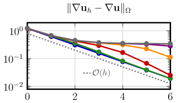
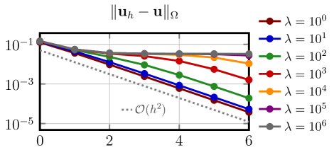
Figure 1. Discretization errors for the method (M1), $k=1$, under mesh refinement ($x$-axis: refinement level $L$) and different values of $\lambda$ for Example 1.

For successively refined meshes with smallest edge length $h=2^{-(L+2)}$, fixed polynomial degree $k=1$ and levels $L=0,..,6$ we compute the error $\boldsymbol{u}-\boldsymbol{u}_{h}$ in the $L^{2}$ norm and the $H^{1}$ semi-norm for different values of $\lambda$. The absolute errors are displayed in Figure 1. Let us emphasize that the solution $\boldsymbol{u}$ is independent of $\lambda$. For fixed and moderate $\lambda$ we observed the expected convergence rates, i.e. second order in the $L^{2}$ norm and first order in the $H^{1}$ norm. However, we observe that the error is severely depending on $\lambda$. Especially for larger values of $\lambda$ the asymptotic convergence rates for $h\to 0$ are shifted to finer resolutions; for instance, for $\lambda=10^{5}$ convergence can not yet be observed on the chosen meshes. Overall, we observe an error behavior of the form $\mathcal{O}(\lambda\cdot h^{k})$ for the $H^{1}$ semi-norm and $\mathcal{O}(\lambda\cdot h^{k+1})$ for the $L^{2}$ norm. From the discretization (M1) we directly see that with increasing $\lambda$ we enforce that $\operatorname{\operatorname{div}}\boldsymbol{u}$ tends to zero (pointwise). For piecewise linear functions, however, the only divergence-free function that can be represented is the constant function. This leads to the observed effect which is known as volume-locking. We give a brief definition here:

Volume-locking is a structural property of the discrete finite element spaces involved. In the limit case $\lambda\to\infty$, one expects that the limit displacement $\boldsymbol{u}$ is divergence-free. Recalling (3a) and introducing the discrete counterpart

$$\boldsymbol{V}^{0}_{h}:=\left\{\boldsymbol{v}_{h}\in\boldsymbol{P}_{\!h,0}^{k}:\operatorname{\operatorname{div}}_{h}\,\boldsymbol{v}_{h}=0\right\},$$ (7)

where $\operatorname{\operatorname{div}}_{h}$ is a discretized $\operatorname{\operatorname{div}}$ operator, one is ready for a precise definition of volume-locking:

Definition 1.

Volume-locking means that the discrete subspace of discretely divergence-free vector fields of $\boldsymbol{V}^{0}_{h}$ does not have optimal approximation properties versus smooth, divergence-free vector fields $\boldsymbol{v}\in\boldsymbol{V}^{0}\cap\boldsymbol{H}^{k+1}(\Omega)$

$$\inf_{\boldsymbol{v}_{h}\in\boldsymbol{V}^{0}_{h}}\|\nabla\boldsymbol{v}-\nabla\boldsymbol{v}_{h}\|_{\Omega}\not\leq Ch^{k}|\boldsymbol{v}|_{k+1},$$ (8a)

although the entire vector-valued finite element space $$\boldsymbol{P}_{\!h,0}^{k}$$ possesses optimal approximation properties of the form

$$\inf_{\boldsymbol{v}_{h}\in\boldsymbol{P}_{\!h,0}^{k}}\|\nabla\boldsymbol{v}-\nabla\boldsymbol{v}_{h}\|_{\Omega}\leq Ch^{k}|\boldsymbol{v}|_{k+1}.$$ (8b)

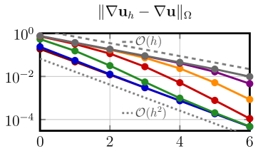
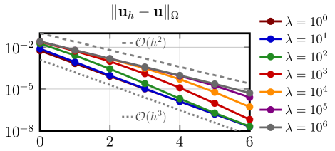
Figure 2. Discretization errors for the method (M1), $k=2$, under mesh refinement ($x$-axis: refinement level $L$) and different values of $\lambda$ for Example 1.

In the sense of Definition 1 the discretization (M1) with $k=1$ is obviously not free of volume-locking. The problem can be alleviated by going to higher order, cf. Figure 2 for the same problem and discretization but with order $k=2$. We observe that convergence is secured in this case also for the highest values of $\lambda$. However, the discretization error still depends strongly on $\lambda$ and for large $\lambda$ and insufficiently fine mesh sizes $h$ an order drop can be observed. The overall convergence behaves like $\mathcal{O}(\min\{h^{k-1},\lambda h^{k}\})$ for the $H^{1}$ semi-norm and $\mathcal{O}(\min\{h^{k},\lambda h^{k+1}\})$ for the $L^{2}$ norm. Hence, even for $k=2$ the discretization (M1) is not free of volume-locking.

2.2. A volume-locking-free discretization through mixed formulation

To get rid of the locking-effect one often reformulates the grad-div term in (1) by rewriting the problem in mixed form as

$$-\operatorname{\operatorname{div}}\left(2\mu\nabla_{s}\boldsymbol{u}\right)-\nabla p =\boldsymbol{f}\qquad \Omega$$ in , (9a)

$$\operatorname{\operatorname{div}}\boldsymbol{u}+\lambda^{-1}p =0\qquad \Omega$$ in , (9b)

Here, the auxiliary variable $p$ approximating $\lambda\operatorname{\operatorname{div}}\boldsymbol{u}$ is introduced. In the limit $\lambda\to\infty$ this yields an incompressible Stokes problem. With the intention to avoid volume-locking we now consider a discretization that is known to be stable in the Stokes limit. Here, we take the well-known Taylor-Hood velocity-pressure pair: Find $(\boldsymbol{u}_{h},p_{h})\in\boldsymbol{P}_{\!h,0}^{k}\times P_{\!h}^{k-1}$, s.t.

$$\int_{\Omega}2\mu\,\nabla_{s}(\boldsymbol{u}_{h}):\nabla_{s}(\boldsymbol{v}_{h})\,\mathrm{d}\boldsymbol{x}+\int_{\Omega}\operatorname{\operatorname{div}}(\boldsymbol{v}_{h})p_{h}\,\mathrm{d}\boldsymbol{x} =\int_{\Omega}\boldsymbol{f}\!\cdot\!\boldsymbol{v}\,\,\mathrm{d}\boldsymbol{x}\quad \forall~{}v_{h}\in\boldsymbol{P}_{\!h,0}^{k},$$ (M2a)

$$\int_{\Omega}\operatorname{\operatorname{div}}(\boldsymbol{u}_{h})q_{h}\,\mathrm{d}\boldsymbol{x}-\int_{\Omega}\lambda^{-1}p_{h}q_{h}\,\mathrm{d}\boldsymbol{x} =0\quad \forall~{}q_{h}\in P_{\!h}^{k-1}.$$ (M2b)

It is well-known that for every LBB-stable Stokes discretization the mixed formulation of linear elasticity guarantees that the discretization is free of volume-locking in the sense of Definition 1, cf. [11, Chapter VI.3].

Let us note that we can interprete (M2b) as $p_{h}=\lambda\Pi_{P_{\!h}}\operatorname{\operatorname{div}}(\boldsymbol{u}_{h})$ where $\Pi_{P_{\!h}}$ is the $L^{2}(\Omega)$ projection into $P_{\!h}^{k-1}$. Hence, we can formally rewrite (M2) as: Find $\boldsymbol{u}_{h}\in\boldsymbol{P}_{\!h,0}^{k}$ s.t.

$$\int_{\Omega}2\mu\,\nabla_{s}(\boldsymbol{u}_{h}):\nabla_{s}(\boldsymbol{v}_{h})\,\mathrm{d}\boldsymbol{x}+\int_{\Omega}\lambda\,\Pi_{P_{\!h}}\operatorname{\operatorname{div}}(\boldsymbol{u}_{h})\operatorname{\operatorname{div}}(\boldsymbol{v}_{h})\,\mathrm{d}\boldsymbol{x}=\int_{\Omega}\boldsymbol{f}\cdot\boldsymbol{v}\,\,\mathrm{d}\boldsymbol{x}.$$ (M2*)

We note that the only difference between (M2*) and (M1) is in the projection $\Pi_{P_{\!h}}$. Hence, the $\operatorname{\operatorname{div}}_{h}$ in a corresponding subspace $\boldsymbol{V}^{0}_{h}$ is different,

$$\boldsymbol{V}^{0}_{h}:=\left\{\boldsymbol{v}_{h}\in\boldsymbol{P}_{\!h,0}^{k}:\Pi_{P_{\!h}}\operatorname{\operatorname{div}}\left(\boldsymbol{v}_{h}\right)=0\right\},$$

yielding a much richer space $\boldsymbol{V}^{0}_{h}$ to approximate with. The scheme (M2*) can be considered as an improvement over the plain scheme (M1) using a reduced integration [30] for the grad-div term to avoid volume-locking. See [39] for a discussion of the equivalence of certain mixed finite element methods with displacement methods which use the reduced and selective integration technique.

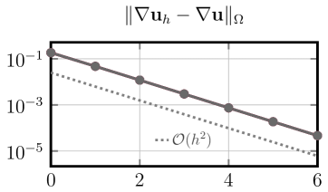
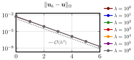
Figure 3. Discretization errors for the method (10), $k=2$, under mesh refinement ($x$-axis: refinement level $L$) and different values of $\lambda$ for Example 1.

In Figure 3 we display the results of the previous numerical experiment with the method in (M2a)–(M2b). We observe that indeed, the discretization error is essentially independent of $\lambda$ and optimally convergent.

2.3. Gradient-robustness

In the previous subsection we considered a divergence-free force field. As a result of the Helmholtz decomposition we can decompose every $L^{2}$ force field into a divergence-free and an irrotational part. In this section we now consider the case where the force field is irrotational, i.e. a gradient of an $H^{1}$ function. This will lead us to the formulation of gradient-robustness. Assume that there is $\phi\in H^{1}(\Omega)$ with $\int\phi\,\mathit{dx}=0$ so that $\boldsymbol{f}=\nabla\phi$. With $\lambda\to\infty$ we have $p\to\phi$ and $\boldsymbol{u}\to\boldsymbol{0}$ , i.e. in the Stokes limit gradients in the force field are solely balanced by the pressure and have no impact on the displacement. In the next subsection, this reasoning will be made more precise by deriving an asymptotic result in the limit $\lambda\to\infty$.

2.4. A definition of gradient-robustness

First, we introduce the orthogonal complement of the weakly-differential divergence-free vector fields (3a) with respect to the inner-product $a(\cdot,\cdot)$ defined in (M1):

$$\boldsymbol{V}^{\perp}:=\{\boldsymbol{u}\in\boldsymbol{H}^{1}_{0}(\Omega):a(\boldsymbol{u},\boldsymbol{v})=0,\forall\boldsymbol{v}\in\boldsymbol{V}^{0}\}.$$ (11)

Then, the solution of the linear elasticity equation can be decomposed as

$$\boldsymbol{u}=\boldsymbol{u}^{0}+\boldsymbol{u}^{\perp},\qquad\boldsymbol{u}^{0}\in\boldsymbol{V}^{0},\quad\boldsymbol{u}^{\perp}\in\boldsymbol{V}^{\perp},$$ (12)

where $\boldsymbol{u}^{0}$ satisfies

$$a(\boldsymbol{u}^{0},\boldsymbol{v}^{0})=a(\boldsymbol{u},\boldsymbol{v}^{0})=(\boldsymbol{f},\boldsymbol{v}^{0}),\quad\forall\boldsymbol{v}^{0}\in\boldsymbol{V}^{0}.$$ (13)

The following lemma characterizes a robustness property of exact solutions to linear elasticity problems.

Theorem 1 (Gradient-robustness of nearly incompressible materials).

If the right hand side $\boldsymbol{f}\in H^{-1}(\Omega)$ in (1a) is a gradient field, i.e. $\boldsymbol{f}=\nabla\phi$, $\phi\in L^{2}(\Omega)$, then it holds for the solution $\boldsymbol{u}=\boldsymbol{u}^{0}+\boldsymbol{u}^{\perp}$ of (1) (under homogeneous Dirichlet boundary conditions)

$$\boldsymbol{u}^{0}=0,\qquad\boldsymbol{u}^{\perp}=\mathcal{O}(\lambda^{-1}),$$

i.e., for $\lambda\to\infty$ one gets $\boldsymbol{u}=\boldsymbol{u}^{\perp}\to\boldsymbol{0}$.

Proof.

Taking $\boldsymbol{v}^{0}=\boldsymbol{u}^{0}$ in equation (13), we get

$$a(\boldsymbol{u}^{0},\boldsymbol{u}^{0})=(\boldsymbol{f},\boldsymbol{u}^{0})=(\nabla\phi,\boldsymbol{u}^{0})=(-\phi,\operatorname{\operatorname{div}}(\boldsymbol{u}^{0}))=0.$$

Hence, $\boldsymbol{u}^{0}=0$.

On the other hand we obtain

$$(2\mu\,\nabla_{s}(\boldsymbol{u}^{\perp}),\nabla_{s}(\boldsymbol{u}^{\perp}))+(\lambda\,\operatorname{\operatorname{div}}\boldsymbol{u}^{\perp},\operatorname{\operatorname{div}}\boldsymbol{u}^{\perp}) =\boldsymbol{f}(\boldsymbol{u}^{\perp})$$

$$=-(\phi,\operatorname{\operatorname{div}}\boldsymbol{u}^{\perp}) \leq\|\phi\|_{L^{2}(\Omega)}\|\boldsymbol{u}^{\perp}\|_{H^{1}(\Omega)}.$$

From Korn’s inequality $\|\boldsymbol{u}^{\perp}\|_{H^{1}(\Omega)}^{2}\leq C(2\nabla_{s}(\boldsymbol{u}^{\perp}),\nabla_{s}(\boldsymbol{u}^{\perp})),$ and an estimate on the $H^{1}$ norm of functions in $\boldsymbol{V}^{\perp}$, $\|\boldsymbol{u}^{\perp}\|_{H^{1}(\Omega)}\leq\beta\|\operatorname{\operatorname{div}}\boldsymbol{u}^{\perp}\|_{L^{2}(\Omega)}$, where $C$ is the constant for the Korn’s inequality and $\beta$ is the inf-sup constant of a corresponding Stokes problem, cf. [28, Corollary 3.47], we hence have

$$(\frac{\mu}{C}+\frac{\lambda}{\beta})\|\boldsymbol{u}^{\perp}\|_{H^{1}(\Omega)}\leq\|\phi\|_{L^{2}(\Omega)},$$

from which we conclude the statement. ∎

The previous characterization does not automatically carry over to discretization schemes.

Definition 2.

We denote a space discretization for the linear elasticity equation which fulfills an analogue to Theorem 1 also discretely as gradient-robust, i.e., gradient-robustness means for a discretization of (1) that in the limit $\lambda\to\infty$ it holds $\boldsymbol{u}_{h}=\mathcal{O}(\lambda^{-1})$.

Remark 1 (Gradient robustness for the Stokes limit).

Gradient-robustness is directly related to the concept of pressure robustness in the Stokes case. Actually, a gradient-robust discretization for the linear elasticity problem (1) is asymptotic preserving (AP) in the sense of [27] such that for $\lambda\to\infty$ the space discretization converges on every (fixed) grid to a pressure-robust space discretization of the (formal) Stokes problem (4).

It is known that the standard Taylor-Hood discretization is not pressure-robust. However, several discretizations for the Stokes problem exists that are pressure-robust [29] or can be made pressure-robust by a suitable modification [36]. We demonstrate the consequences for the linear elasticity problem in the following, where the forcing $\boldsymbol{f}$ is a gradient field.

Example 2.

We take $\boldsymbol{f}=\nabla\phi$ with $\phi=x^{6}+y^{6}$. and (homogeneous) Dirichlet boundary conditions so that it holds $\boldsymbol{u}\to\boldsymbol{0}$ in the asymptotic limit $\lambda\to\infty$.

We now compare the different methods on a fixed grid (or a couple of fixed grids) and we investigate the norm of the solution $\boldsymbol{u}$ with respect to $\lambda\to\infty$. For gradient-robust methods this norm should vanish as $\mathcal{O}(\lambda^{-1})$ independent of $h$. For methods that are not gradient-robust the limit will be $\mathcal{O}(h^{k})$ for $\lambda\to\infty$ depending on the mesh size $h$ and the order $k$. The results for the methods (M1) and (M2a)–(M2b) for Example 2, are shown in Fig. 4. While (M1) behaves well as $\|\nabla\boldsymbol{u}_{h}\|_{\Omega}$ goes to zero with $\lambda^{-1}$ essentially independent of $h$, for the method in (M2a)–(M2b) we observe a lower bound for $\|\nabla\boldsymbol{u}_{h}\|_{\Omega}$ that depends on the mesh.

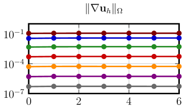
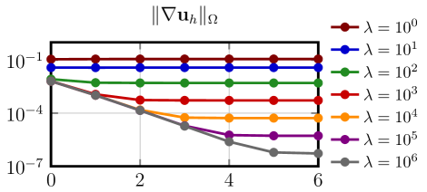
Figure 4. Norm of discrete solution for methods in (M1) (left) and (M2a)–(M2b) (right), $k=2$, under mesh refinement ($x$-axis: refinement level $L$) and different values of $\lambda$ for Example 2.

As a conclusion of the numerical examples, let us summarize that both basic methods that we considered here, the discretization (M1) and the Taylor-Hood based method in (M2a)–(M2b) are not satisfactory. While (M1) seems to be gradient-robust it is not free of volumetric locking while the behavior of the Taylor-Hood based method in (M2a)–(M2b) has the exact opposite properties.

Remark 2.

In the first example we considered a divergence-free forcing. The observations stay essentially the same if more general forcings are considered there, e.g. if the solutions of both examples are superimposed.

2.5. The basic method on barycentric refined meshes

A comparably simple discretization scheme that is known to be pressure robust for the Stokes limit is the Scott-Vogelius element [44, 46], which is the classical Taylor-Hood discretization with a discontinuous pressure space. However, this discretization is known to be LBB-stable (and hence free of volume-locking) only for special triangulations or sufficiently high orders. Applications of this element to linear elasticity have been made for example in [40]. Let us consider the last two examples again, but on every level we apply a barycentrical refinement of the original mesh by connecting all vertices of the mesh cell with the barycenter of this mesh cell, cf. Figure 5.

Figure 5. Barycentric-refined triangular mesh on the unit square with refinement level $L=0$.

If we apply the basic method (M1) in this case with $k\geq 2$ we have a gradient-robust scheme which at the same time has a sufficiently large discretely divergence-free subspace $\boldsymbol{V}_{h}^{0}$ to be volume-locking free. The results are given in Figure 6 and are consistent with these expectations.

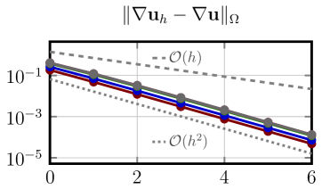
Figure 6. Discretizaton error for Example 1 (left) and norm of discrete error for Example 2 (right) for the method (M1), $k=2$, on a barycentric-refined mesh under mesh refinement ($x$-axis: refinement level $L$) and different values of $\lambda$ for Example 2.

3. $H(\operatorname{\operatorname{div}})$-conforming HDG Discretization and Analysis

In the remainder of this paper we consider a special class of discretizations for linear elasticity: $H(\operatorname{\operatorname{div}})$-conforming HDG discretizations where we also keep track of the volume-locking and gradient-robustness property of the method. In Subsections 3.1 – 3.3 we introduce preliminaries, notation and the numerical method and analyse it with respect to quasi-optimal error estimates and volume-locking in Subsection 3.4. The prove of gradient-robustness is carried out in Subsection 3.5. Numerical results support these theoretical findings in Subsection 3.6. In the subsequent section, Section 4, we consider a (more efficient) modified scheme which is volume-locking free, but is gradient-robust only after a simple modification.

3.1. Preliminaries

Let $\mathcal{F}_{h}=\{F\}$ be the collection of facets (edges in 2D, faces in 3D) in $\mathcal{T}_{h}$. We distinguish functions with support only on facets indicated by a subscript $F$ and those with support also on the volume elements which is indicated by a subscript $T$. Compositions of both types are used for the HDG discretization of the displacement and indicated by underlining, $\underline{\boldsymbol{u}}=(\boldsymbol{u}_{T},\boldsymbol{u}_{F})$. On each simplex $T$, we denote the tangential component of a vector $\boldsymbol{v}_{T}$ on a facet $F$ by $(\boldsymbol{v}_{T})^{t}=\boldsymbol{v}_{T}-(\boldsymbol{v}_{T}\cdot\boldsymbol{n})\boldsymbol{n}$, where $\boldsymbol{n}$ is the unit normal vector on $F$. Furthermore, we denote the compound exact solution as $\underline{\boldsymbol{u}}:=(\boldsymbol{u},\boldsymbol{u}^{t})$, and introduce the composite space of sufficiently smooth functions

$$\underline{\boldsymbol{U}\!}(h):=[H^{2}_{0}(\Omega)]^{d}\times[H^{1}_{0}(\mathcal{F}_{h})]^{d}.$$ (14)

3.2. Finite elements

We consider an HDG method which approximates the displacement on the mesh $\mathcal{T}_{h}$ using an $H(\operatorname{\operatorname{div}})$-conforming space and the tangential component of the displacement on the mesh skeleton $\mathcal{F}_{h}$ with a DG facet space given as follows:

$$\boldsymbol{V}_{\!h}:= \;\{\boldsymbol{v}_{T}\in\prod_{T\in\mathcal{T}_{h}}[\mathbb{P}^{k}(T)]^{d}:\;\;[\![\boldsymbol{v}_{T}\cdot\boldsymbol{n}]\!]_{F}=0\,\forall F\in\mathcal{F}_{h}\}\subset H_{0}(\operatorname{\operatorname{div}},\Omega),$$ (15a)

$$M_{h}:= \;\{\boldsymbol{v}_{F}\in\prod_{F\in\mathcal{F}_{h}}M_{k}(F):\;\;\boldsymbol{v}_{F}\cdot\boldsymbol{n}=0\,\forall F\in\mathcal{F}_{h},\;\;\boldsymbol{v}_{F}=0\,\;\;\forall F\subset\partial\Omega\},$$ (15b)

where $$[\![\cdot]\!] \mathbb{P}^{k} k$$ is the usual jump operator, the space of polynomials up to degree , and

$$M_{k}(F):=\left\{\begin{tabular}[]{l l}$[\mathbb{P}^{0}(F)]^{3}\oplus\boldsymbol{x}\times[\mathbb{P}^{0}(F)]^{3}$&if $k=1$ and $d=3$,\vspace{.2cm}\\ $[\mathbb{P}^{k-1}(F)]^{d}$&else.\end{tabular}\right.$$

Note that functions in $$M_{h}$$ are defined only on the mesh skeleton and have normal component zero.

To further simplify notation, we denote the composite space as

$$\underline{\boldsymbol{U}\!}_{h}:=\boldsymbol{V}_{\!h}\times{M}_{h}.$$

3.3. The numerical scheme

We introduce the $L^{2}$ projection onto $M_{k}(F)$ $\Pi_{M}$:

$$\Pi_{M}:[L^{2}(F)]^{d}\rightarrow M_{k}(F),\quad\int_{F}(\Pi_{M}f)v\,\mathrm{ds}=\int_{F}f\,v\,\mathrm{ds}\quad\forall v\in M_{k}(F).$$

Then, for all $\underline{\boldsymbol{u}},\underline{\boldsymbol{v}}\in\underline{\boldsymbol{U}\!}_{h}$, we introduce the bilinear and linear forms

$$a_{h}(\underline{\boldsymbol{u}},\underline{\boldsymbol{v}}):= \;a_{h}^{\mu}(\underline{\boldsymbol{u}},\underline{\boldsymbol{v}})+a_{h}^{\lambda}(\underline{\boldsymbol{u}},\underline{\boldsymbol{v}})$$ (16a)

$$a_{h}^{\mu}(\underline{\boldsymbol{u}},\underline{\boldsymbol{v}}):= \;\sum_{T\in\mathcal{T}_{h}}\int_{T}2\mu\,\nabla_{s}(\boldsymbol{u}_{T}):\nabla_{s}(\boldsymbol{v}_{T})\,\mathrm{d}\boldsymbol{x}$$ (16b)

$$\;-\int_{\partial T}2\mu\,\nabla_{s}(\boldsymbol{u}_{T})\boldsymbol{n}\cdot[\![\underline{\boldsymbol{v}}^{t}]\!]\,\mathrm{d}\boldsymbol{s}-\int_{\partial T}2\mu\,\nabla_{s}(\boldsymbol{v}_{T})\boldsymbol{n}\cdot[\![\underline{\boldsymbol{u}}^{t}]\!]\,\mathrm{d}\boldsymbol{s}$$

$$\;+\int_{\partial T}\mu\frac{\alpha}{h}\Pi_{M}[\![\underline{\boldsymbol{u}}^{t}]\!]\cdot\Pi_{M}[\![\underline{\boldsymbol{v}}^{t}]\!]\,\mathrm{d}\boldsymbol{s},$$

$$a_{h}^{\lambda}(\underline{\boldsymbol{u}},\underline{\boldsymbol{v}}):= \;\sum_{T\in\mathcal{T}_{h}}\int_{T}\lambda\,\operatorname{\operatorname{div}}(\boldsymbol{u}_{T})\operatorname{\operatorname{div}}(\boldsymbol{v}_{T})\,\mathrm{d}\boldsymbol{x},$$ (16c)

$$f(\underline{\boldsymbol{v}}):= \;\sum_{T\in\mathcal{T}_{h}}\int_{T}\boldsymbol{f}\cdot\boldsymbol{v}_{T}\,\mathrm{d}\boldsymbol{x}.$$ (16d)

where $$[\![\underline{\boldsymbol{u}}^{t}]\!]=(\boldsymbol{u}_{T})^{t}-\boldsymbol{u}_{F} \alpha=\alpha_{0}k^{2} \alpha_{0}$$ is the (tangential) jump between element interior and facet unknowns, and with a sufficiently large positive constant.

The numerical scheme then reads: Find $\underline{\boldsymbol{u}}_{h}\in\underline{\boldsymbol{U}\!}_{h}$ such that

$$a_{h}(\underline{\boldsymbol{u}}_{h},\underline{\boldsymbol{v}}_{h})=f(\underline{\boldsymbol{v}}_{h}),\quad\forall\underline{\boldsymbol{v}}_{h}\in\underline{\boldsymbol{U}\!}_{h}.$$ (S1)

3.4. Error estimates

We write

$$A\preceq B$$

to indicate that there exists a constant $C$, independent of the mesh size $h$, the Lamé parameters $\mu$ and $\lambda$, and the numerical solution, such that $A\leq CB.$

Denote the space of rigid motions

$$RM(T)=\{\boldsymbol{a}+B\,\boldsymbol{x}:\;\;\boldsymbol{a}\in\mathbb{R}^{d},B\in S_{d}\},$$

where $S_{d}$ is the space of anti-symmetric $d\times d$ matrices. We observe that the tangential trace on a facet $F$ of any function in $RM(T)$ is a constant in 2D, and lies in the space $M_{1}(F)$ in 3D. Hence, there holds

$$\boldsymbol{v}^{t}|_{F}\in M_{k}(F),\quad\quad\forall\boldsymbol{v}\in RM(T).$$ (17)

The above property is the key to prove coercivity of the bilinear form (16a).

We use the following projection $\Pi_{RM}$ from $[H^{1}(T)]^{d}$ onto $RM(T)$ [12]:

$$\int_{T}\Pi_{RM}\boldsymbol{u}\,\mathrm{d}\boldsymbol{x}= \;\int_{T}\boldsymbol{u}\,\mathrm{d}\boldsymbol{x},$$

$$\int_{T}{{{\boldsymbol{\mathrm{curl}}}}}\,(\Pi_{RM}\boldsymbol{u})\,\mathrm{d}\boldsymbol{x}= \;\int_{T}{{{\boldsymbol{\mathrm{curl}}}}}\,\boldsymbol{u}\,\mathrm{d}\boldsymbol{x},$$

where ${{{\boldsymbol{\mathrm{curl}}}}}\,\boldsymbol{u}$ is the anti-symmetric part of the gradient of $\boldsymbol{u}$. Following [12] this projection operator has the approximation properties

$$||{\nabla}(\boldsymbol{u}-\Pi_{RM}\boldsymbol{u})||_{T}\preceq \;||\nabla_{s}(\boldsymbol{u})||_{T},$$ (18a)

$$||\boldsymbol{u}-\Pi_{RM}\boldsymbol{u}||_{T}\preceq \;h_{T}||{\nabla}(\boldsymbol{u}-\Pi_{RM}\boldsymbol{u})||_{T}.$$ (18b)

Denoting the following (semi)norms

$$\|\underline{\boldsymbol{v}}\|_{\mu,h}:=\mu^{\frac{1}{2}}\|\underline{\boldsymbol{v}}\|_{1,h},\quad\|\underline{\boldsymbol{v}}\|_{\mu,*,h}:=\mu^{\frac{1}{2}}\|\underline{\boldsymbol{v}}\|_{1,*,h},\quad\|\underline{\boldsymbol{v}}\|_{\mu,**,h}:=\mu^{\frac{1}{2}}\|\underline{\boldsymbol{v}}\|_{1,**,h},$$

$$\|\underline{\boldsymbol{v}}\|_{1,h}:= \;\left(\sum_{T\in\mathcal{T}_{h}}2\|\nabla_{s}\boldsymbol{v}_{T}\|^{2}_{T}+\frac{2}{h}\|\Pi_{M}[\![\underline{\boldsymbol{v}}^{t}]\!]\|^{2}_{\partial T}\right)^{1/2},$$ (19a)

$$\|\underline{\boldsymbol{v}}\|_{1,*,h}:= \;\Big{(}\|\underline{\boldsymbol{v}}\|_{1,h}^{2}+\sum_{T\in\mathcal{T}_{h}}2h\|\nabla_{s}(\boldsymbol{v}_{T})\boldsymbol{n}\|^{2}_{\partial T}\Big{)}^{1/2},$$ (19b)

$$\|\underline{\boldsymbol{v}}\|_{1,**,h}:= \;\Big{(}\|\underline{\boldsymbol{v}}\|_{1,*,h}^{2}+\sum_{T\in\mathcal{T}_{h}}\frac{2}{h}\|[\![\underline{\boldsymbol{v}}^{t}]\!]\|^{2}_{\partial T}\Big{)}^{1/2}.$$ (19c)

We also denote the $H^{s}$-norm on $\Omega$ as $\|\cdot\|_{s}$, and when $s=0$, we simply denote $\|\cdot\|$ as the $L^{2}$-norm on $\Omega$.

To derive optimal $L^{2}$ error estimates, we shall assume the following full $H^{2}$-regularity

$$\mu\|\boldsymbol{\phi}\|_{2}+\lambda\|\operatorname{\operatorname{div}}\,\boldsymbol{\phi}\|_{1}\preceq\|\boldsymbol{\theta}\|$$ (20)

for the dual problem with any source term $\boldsymbol{\theta}\in[L^{2}(\Omega)]^{d}$:

$$-\operatorname{\operatorname{div}}\left(2\mu\nabla_{s}\boldsymbol{\phi}\right)-{\nabla}\left(\lambda\,\operatorname{\operatorname{div}}\boldsymbol{\phi}\right)= \;\boldsymbol{\theta}\quad\text{ in }\Omega,$$ (21a)

$$\boldsymbol{\phi}= \;\boldsymbol{0}\quad\text{ on }\partial\Omega.$$ (21b)

The estimate (20) holds on convex polygons [13].

We have the following estimates.

Theorem 2.

Assume $k\geq 1$ and the regularity $\boldsymbol{u}\in[H^{k+1}(\Omega)]^{d}$. Let $\underline{\boldsymbol{u}}_{h}\in\underline{\boldsymbol{U}\!}_{h}$ be the numerical solution to the scheme (S1). Then, for sufficiently large stabilization parameter $\alpha_{0}$, the following estimate holds

$$\|\underline{\boldsymbol{u}}-\underline{\boldsymbol{u}}_{h}\|_{\mu,h}\preceq \;\mu^{1/2}h^{k}\|\boldsymbol{u}\|_{k+1},$$ (22a)

$$\|\operatorname{\operatorname{div}}(\boldsymbol{u}-\boldsymbol{u}_{T})\|\preceq \;(\mu/\lambda)^{1/2}h^{k}\|\boldsymbol{u}\|_{k+1}+h^{k}\|\operatorname{\operatorname{div}}\,\boldsymbol{u}\|_{k}.$$ (22b)

Moreover, under the regularity assumption (20), the following estimate holds

$$\|\boldsymbol{u}-\boldsymbol{u}_{T}\|\preceq h^{k+1}\|\boldsymbol{u}\|_{k+1}.$$ (22c)

Remark 3 (Volume-locking-free estimates).

From the energy estimates (22a), we get that

$$\sum_{T\in\mathcal{T}_{h}}\|\nabla_{s}(\boldsymbol{u}-\boldsymbol{u}_{h,T})\|^{2}_{T}+\frac{1}{h}\|\Pi_{M}[\![(\underline{\boldsymbol{u}}-\underline{\boldsymbol{u}}_{h})^{t}]\!]\|^{2}_{\partial T}\preceq h^{2k}\|\boldsymbol{u}\|_{k+1}^{2},$$

with the hidden constant independent of the Lamé constants $\lambda$ and $\mu$. This observation also holds for the $L^{2}$-norm estimate (22c). Hence, the estimates are free of volume-locking when $\lambda\rightarrow+\infty$.

Proof.

We proceed in the following five steps.

Step 1 (Coercivity): Observing the definition (16a) for the bilinear form $a_{h}^{\mu}(\cdot,\cdot)$, and applying the Cauchy-Schwarz inequality combined with trace-inverse inequalities, we obtain, cf. [20, Lemma 2], for sufficiently large $\alpha$,

$$\|\underline{\boldsymbol{v}}_{h}\|_{\mu,h}^{2}\preceq a_{h}^{\mu}(\underline{\boldsymbol{v}}_{h},\underline{\boldsymbol{v}}_{h})\quad\forall\underline{\boldsymbol{v}}_{h}\in\underline{\boldsymbol{U}\!}_{h}.$$ (23)

Step 2 (Norm equivalence): By property (17), we have $\Pi_{M}(\Pi_{RM}\boldsymbol{v}_{T})^{t}=(\Pi_{RM}\boldsymbol{v}_{T})^{t}$. Hence, for any interior facet $F\in\mathcal{F}_{h}\backslash\partial\Omega$ and any function $\underline{\boldsymbol{v}}\in\underline{\boldsymbol{U}\!}(h)+\underline{\boldsymbol{U}\!}_{h}$, we have

$$\|[\![\underline{\boldsymbol{v}}^{t}]\!]\|_{F}\leq \;\|\Pi_{M}[\![\underline{\boldsymbol{v}}^{t}]\!]\|_{F}+\|\boldsymbol{v}_{T}^{t}-\Pi_{M}\boldsymbol{v}_{T}^{t}\|_{F}$$

$$\leq \;\|\Pi_{M}[\![\underline{\boldsymbol{v}}^{t}]\!]\|_{F}+\|(\boldsymbol{v}_{T}-\Pi_{RM}\boldsymbol{v}_{T})^{t}-\Pi_{M}(\boldsymbol{v}_{T}-\Pi_{RM}\boldsymbol{v}_{T})^{t}\|_{F}$$

$$\preceq \;\|\Pi_{M}[\![\underline{\boldsymbol{v}}^{t}]\!]\|_{F}+\|\boldsymbol{v}_{T}-\Pi_{RM}\boldsymbol{v}_{T}\|_{F}.$$

Using the trace theorem and approximation properties (18) of the projector $\Pi_{RM}$, we get

$$\|\boldsymbol{v}_{T}-\Pi_{RM}\boldsymbol{v}_{T}\|_{F}^{2}\preceq \;\sum_{T\in\mathcal{T}(F)}(h|\boldsymbol{v}_{T}-\Pi_{RM}\boldsymbol{v}_{T}|^{2}_{1,T}+h^{-1}\|\boldsymbol{v}_{T}-\Pi_{RM}\boldsymbol{v}_{T}\|^{2}_{T})$$

$$\preceq \;h\,\|\nabla_{s}\boldsymbol{v}_{T}\|^{2}_{\mathcal{T}(F)},$$

where $\mathcal{T}(F)$ is the set of the two simplexes meeting $F$. Hence,

$$\|[\![\underline{\boldsymbol{v}}^{t}]\!]\|_{F}\leq \;\|\Pi_{M}[\![\underline{\boldsymbol{v}}^{t}]\!]\|_{F}+h^{1/2}\,\|\nabla_{s}\boldsymbol{v}_{T}\|_{\mathcal{T}(F)}\quad\quad\forall\underline{\boldsymbol{v}}\in\underline{\boldsymbol{U}\!}(h)+\underline{\boldsymbol{U}\!}_{h}.$$ (24)

Recally the norms defined in (19), this directly implies

$$\|\underline{\boldsymbol{v}}\|_{\mu,**,h}\preceq\|\underline{\boldsymbol{v}}\|_{\mu,*,h}\quad\quad\forall\underline{\boldsymbol{v}}\in\underline{\boldsymbol{U}\!}(h)+\underline{\boldsymbol{U}\!}_{h}.$$ (25a)

On the other hand, by trace and inverse inequalities, we have, cf. [20, Lemma 1],

$$\|\underline{\boldsymbol{v}}_{h}\|_{\mu,*,h}\preceq\|\underline{\boldsymbol{v}}_{h}\|_{\mu,h}\quad\quad\forall\underline{\boldsymbol{v}}_{h}\in\underline{\boldsymbol{U}\!}_{h}.$$ (25b)

Step 3 (Boundedness): Applying the Cauchy-Schwarz inequality on the bilinear form $a_{h}(\cdot,\cdot)$, we obtain using the estimate (24)

$$a_{h}^{\mu}(\underline{\boldsymbol{v}},\underline{\boldsymbol{w}})\leq \;\|\underline{\boldsymbol{v}}\|_{\mu,**,h}\|\underline{\boldsymbol{w}}\|_{\mu,**,h}\preceq\;\|\underline{\boldsymbol{v}}\|_{\mu,*,h}\|\underline{\boldsymbol{w}}\|_{\mu,*,h}\quad\quad\forall\underline{\boldsymbol{v}},\underline{\boldsymbol{w}}\in\underline{\boldsymbol{U}\!}(h)+\underline{\boldsymbol{U}\!}_{h}.$$ (26)

Step 4 (Galerkin orthogonality, BDM interpolation): Galerkin orthogonality yields $a_{h}(\underline{\boldsymbol{u}},\underline{\boldsymbol{v}}_{h})=f(\underline{\boldsymbol{v}}_{h})$ for all $\underline{\boldsymbol{v}}_{h}\in\underline{\boldsymbol{U}\!}_{h}$. Hence, $a_{h}(\underline{\boldsymbol{u}}-\underline{\boldsymbol{u}}_{h},\underline{\boldsymbol{v}}_{h})=f(\underline{\boldsymbol{v}}_{h})$. We estimate the error by first applying a triangle inequality to split

$$\|\underline{\boldsymbol{u}}-\underline{\boldsymbol{u}}_{h}\|_{\mu,h}\leq\|\underline{\boldsymbol{v}}_{h}-\underline{\boldsymbol{u}}\|_{\mu,h}+\|\underline{\boldsymbol{u}}_{h}-\underline{\boldsymbol{u}}\|_{\mu,h},$$

where we choose $\underline{\boldsymbol{v}}_{h}=(\Pi_{V}\boldsymbol{u},\Pi_{M}\boldsymbol{u})$ where $\Pi_{V}$ is the classical BDM interpolator, [10, Proposition 2.3.2]. We note that the interpolation operator $\Pi_{V}$ has, as a consequence of its commuting diagram property, that

$$\int_{\Omega}\operatorname{\operatorname{div}}(\Pi_{V}\boldsymbol{u}-\boldsymbol{u})q_{h}\,\mathrm{d}\boldsymbol{x}=\int_{\Omega}(\Pi_{Q}\operatorname{\operatorname{div}}\boldsymbol{u}-\operatorname{\operatorname{div}}\boldsymbol{u})q_{h}\,\mathrm{d}\boldsymbol{x}=0\quad\forall~{}q_{h}\in Q_{h},$$

where $\Pi_{Q}$ is the $L^{2}$ projection into $Q_{h}=\prod_{T\in\mathcal{T}_{h}}\mathbb{P}^{k-1}(T)=\operatorname{\operatorname{div}}\boldsymbol{V}_{\!h}$. Hence,

$$\|\underline{\boldsymbol{u}}_{h}-\underline{\boldsymbol{v}}_{h}\|_{\mu,h}^{2}+\lambda\|\operatorname{\operatorname{div}}(\boldsymbol{u}_{T}-\boldsymbol{v}_{T})\|^{2}$$

$$\preceq a_{h}^{\mu}(\underline{\boldsymbol{u}}_{h}-\underline{\boldsymbol{v}}_{h},\underline{\boldsymbol{u}}_{h}-\underline{\boldsymbol{v}}_{h})+\lambda\|\operatorname{\operatorname{div}}(\boldsymbol{u}_{T}-\boldsymbol{v}_{T})\|^{2}$$

$$=a_{h}(\underline{\boldsymbol{u}}_{h}-\underline{\boldsymbol{v}}_{h},\underline{\boldsymbol{u}}_{h}-\underline{\boldsymbol{v}}_{h})=a_{h}(\underline{\boldsymbol{u}}-\underline{\boldsymbol{v}}_{h},\underline{\boldsymbol{u}}_{h}-\underline{\boldsymbol{v}}_{h})$$

$$=a_{h}^{\mu}(\underline{\boldsymbol{u}}-\underline{\boldsymbol{v}}_{h},\;\underline{\boldsymbol{u}}_{h}-\underline{\boldsymbol{v}}_{h})+\underbrace{a_{h}^{\lambda}(\underline{\boldsymbol{u}}-\underline{\boldsymbol{v}}_{h},\;\underline{\boldsymbol{u}}_{h}-\underline{\boldsymbol{v}}_{h})}_{=0}$$

$$\preceq\|\underline{\boldsymbol{u}}-\underline{\boldsymbol{v}}_{h}\|_{\mu,\ast,h}\|\underline{\boldsymbol{u}}_{h}-\underline{\boldsymbol{v}}_{h}\|_{\mu,\ast,h}\preceq\|\underline{\boldsymbol{u}}-\underline{\boldsymbol{v}}_{h}\|_{\mu,\ast,h}\|\underline{\boldsymbol{u}}_{h}-\underline{\boldsymbol{v}}_{h}\|_{\mu,h}.$$

This implies

$$\|\underline{\boldsymbol{u}}-\underline{\boldsymbol{u}}_{h}\|_{\mu,h}+\lambda^{1/2}\|\operatorname{\operatorname{div}}(\boldsymbol{u}_{T}-\boldsymbol{v}_{T})\|\preceq\|\underline{\boldsymbol{u}}-\underline{\boldsymbol{v}}_{h}\|_{\mu,\ast,h}\preceq\mu^{1/2}h^{k}\|\boldsymbol{u}\|_{k+1},$$ (27)

where the last estimate follows from usual Bramble-Hilbert-type arguments, cf. [34, Proposition 2.3.8] for a proof in an almost identical setting. The estimate (22a) follows directly from (27), and the estimate (22b) follows from (27) and the triangle inequality:

$$\|\operatorname{\operatorname{div}}(\boldsymbol{u}-\boldsymbol{u}_{T})\|\leq \;\|\operatorname{\operatorname{div}}(\boldsymbol{u}_{T}-\boldsymbol{v}_{T})\|+\underbrace{\|\operatorname{\operatorname{div}}(\boldsymbol{u}-\boldsymbol{v}_{T})\|}_{=\|(I-\Pi_{Q})\operatorname{\operatorname{div}}\,\boldsymbol{u}\|}$$

$$\preceq \;(\mu/\lambda)^{1/2}h^{k}\|\boldsymbol{u}\|_{k+1}+h^{k}\|\operatorname{\operatorname{div}}\,\boldsymbol{u}\|_{k}.$$

Step 5 (Duality): Let $\boldsymbol{\phi}$ be the solution to the dual problem (21) with $\boldsymbol{\theta}=\boldsymbol{u}-\boldsymbol{u}_{T}$ and $\underline{\boldsymbol{\phi}}=(\boldsymbol{\phi},\boldsymbol{\phi}^{t})\in\underline{\boldsymbol{U}\!}(h)$. By symmetry of the bilinear form $a_{h}(\cdot,\cdot)$ and consistency of the numerical scheme (S1), we have with $\underline{\boldsymbol{\phi}}_{h}=(\Pi_{V}\boldsymbol{\phi},\Pi_{M}\boldsymbol{\phi})\in\underline{\boldsymbol{U}\!}_{h}$

$$\|\boldsymbol{u}-\boldsymbol{u}_{T}\|_{\Omega}^{2} =a_{h}(\underline{\boldsymbol{\phi}},\underline{\boldsymbol{u}}-\underline{\boldsymbol{u}}_{h})=a_{h}(\underline{\boldsymbol{\phi}}-\underline{\boldsymbol{\phi}}_{h},\underline{\boldsymbol{u}}-\underline{\boldsymbol{u}}_{h})$$

$$=a_{h}^{\mu}(\underline{\boldsymbol{\phi}}-\underline{\boldsymbol{\phi}}_{h},\underline{\boldsymbol{u}}-\underline{\boldsymbol{u}}_{h})+a_{h}^{\lambda}(\underline{\boldsymbol{\phi}}-\underline{\boldsymbol{\phi}}_{h},\underline{\boldsymbol{u}}-\underline{\boldsymbol{u}}_{h})$$

$$=a_{h}^{\mu}(\underline{\boldsymbol{\phi}}-\underline{\boldsymbol{\phi}}_{h},\underline{\boldsymbol{u}}-\underline{\boldsymbol{u}}_{h})+\lambda\sum_{T\in\mathcal{T}_{h}}\int_{T}\underbrace{\operatorname{\operatorname{div}}(\boldsymbol{\phi}-\Pi_{V}\boldsymbol{\phi})\operatorname{\operatorname{div}}(\boldsymbol{u}-\Pi_{V}\boldsymbol{u})}_{=(I-\Pi_{Q})\operatorname{\operatorname{div}}\boldsymbol{\phi}\,(I-\Pi_{Q})\operatorname{\operatorname{div}}\boldsymbol{u}}\,\mathrm{d}\boldsymbol{x}$$

$$\preceq\|\underline{\boldsymbol{\phi}}-\underline{\boldsymbol{\phi}}_{h}\|_{\mu,*,h}\|\underline{\boldsymbol{u}}_{h}-\underline{\boldsymbol{u}}\|_{\mu,*,h}+\lambda\|(I-\Pi_{Q})\operatorname{\operatorname{div}}\boldsymbol{\phi}\|\cdot\|(I-\Pi_{Q})\operatorname{\operatorname{div}}\boldsymbol{u}\|$$

$$\preceq\mu h^{k+1}\|\boldsymbol{\phi}\|_{2}\|\boldsymbol{u}\|_{k+1}+\lambda h^{k+1}\|\operatorname{\operatorname{div}}\boldsymbol{\phi}\|_{1}\|\operatorname{\operatorname{div}}\boldsymbol{u}\|_{k}$$

$$\preceq h^{k+1}\|\boldsymbol{u}-\boldsymbol{u}_{T}\|_{\Omega}\|\boldsymbol{u}\|_{k+1},$$

In the last step we invoked the regularity assumption (20). This completes the proof of (22c). ∎

3.5. Gradient-robustness

In this subsection we want to show that the $H(\operatorname{\operatorname{div}})$-conforming HDG method in (S1) is gradient-robust. In this section a splitting into a discretely divergence-free subspace and an orthogonal complement is crucial. To proceed, it seems more natural to work with a DG-equivalent reformulation of the HDG scheme (S1) by eliminating the facet unknowns (for analysis purposes only). In Remark 4 below we explain how this translate to the HDG setting.

We introduce the lifting $\mathcal{L}_{h}:\boldsymbol{V}_{\!h}+[H^{2}_{0}(\Omega)]^{d}\to M_{h}$ where $\mathcal{L}_{h}(\boldsymbol{w}_{T})$ is the unique function in $M_{h}$ such that

$$a_{h}((\boldsymbol{w}_{T},\mathcal{L}_{h}(\boldsymbol{w}_{T}),(0,\boldsymbol{v}_{F}))=0,\quad\forall\boldsymbol{v}_{F}\in M_{h}.$$

For the case of a uniform mesh size $h$, an explicit formula can easily derived yielding

$$\mathcal{L}_{h}(\boldsymbol{w}_{T})=\{\!\!\{\Pi_{M}\boldsymbol{w}_{T}\}\!\!\}_{*}-\frac{h}{2\alpha}[\![\nabla_{s}\boldsymbol{w}_{T}\cdot\boldsymbol{n}]\!]_{*},$$

where $\{\!\!\{\cdot\}\!\!\}_{*}$ and $[\![\cdot]\!]_{*}$ are the usual DG average and jump operators. Then the solution $\underline{\boldsymbol{u}}_{h}=(\boldsymbol{u}_{T},\boldsymbol{u}_{F})\in\underline{\boldsymbol{U}\!}_{h}$ to the scheme (S1) satisfies $\boldsymbol{u}_{F}=\mathcal{L}_{h}(\boldsymbol{u}_{T})$, with $\boldsymbol{u}_{T}\in\boldsymbol{V}_{\!h}$ being the unique function such that

$$\hat{a}_{h}(\boldsymbol{u}_{T},\boldsymbol{v}_{T})=\hat{f}(\boldsymbol{v}_{T})\quad\forall\boldsymbol{v}_{T}\in\boldsymbol{V}_{\!h},$$ (S1-DG)

where $\hat{a}_{h}(\cdot,\cdot)$ and $\hat{f}$ are defined on $\boldsymbol{V}_{\!h}$ as follows:

$$\hat{a}_{h}(\boldsymbol{v}_{T},\boldsymbol{w}_{T}):=a_{h}\left((\boldsymbol{v}_{T},\mathcal{L}_{h}(\boldsymbol{v}_{T})),(\boldsymbol{w}_{T},0)\right),\quad\hat{f}(\boldsymbol{w}_{T}):=f((\boldsymbol{w}_{T},0)),~{}\boldsymbol{v}_{T},\boldsymbol{w}_{T}\in\boldsymbol{V}_{\!h}.$$

Analogously (with slight abuse of notation) we define a norm on $\boldsymbol{V}_{\!h}$ with

$$\|\boldsymbol{u}_{T}\|_{1,h}:=\|(\boldsymbol{u}_{T},\mathcal{L}_{h}(\boldsymbol{u}_{T}))\|_{1,h}.$$

Introducing the spaces

$$\boldsymbol{V}_{\!h}^{0}:=\{\boldsymbol{v}_{T}\in\boldsymbol{V}_{\!h}:\operatorname{\operatorname{div}}\boldsymbol{v}_{T}=0,\quad\forall T\in\mathcal{T}_{h}\},$$ (28a)

and

$$\boldsymbol{V}_{\!h}^{\perp}:=\{\boldsymbol{v}_{T}\in\boldsymbol{V}_{\!h}:\hat{a}_{h}(\boldsymbol{v}_{T},\boldsymbol{w}_{T})=0,\quad\forall\boldsymbol{w}_{T}\in\boldsymbol{V}_{\!h}\}.$$ (28b)

We then split the solution $\boldsymbol{u}_{T}\in\boldsymbol{V}_{\!h}$ to the scheme (S1-DG) as $\boldsymbol{u}_{T}=\boldsymbol{u}_{T}^{0}+\boldsymbol{u}_{T}^{\perp}$ where $\boldsymbol{u}_{T}^{0},\boldsymbol{u}_{T}^{\perp}\in\boldsymbol{V}_{\!h}$ are the unique solutions to the following equations:

$$\hat{a}_{h}(\boldsymbol{u}_{T}^{0},\boldsymbol{v}_{T}^{0}) =\hat{f}(\boldsymbol{v}_{T}^{0})\quad\forall~{}\boldsymbol{v}_{T}^{0}\in\boldsymbol{V}_{\!h}^{0},$$ (29a)

$$\hat{a}_{h}(\boldsymbol{u}_{T}^{\perp},\boldsymbol{v}_{T}^{\perp}) =\hat{f}(\boldsymbol{v}_{T}^{\perp})\quad\forall~{}\boldsymbol{v}_{T}^{\perp}\in\boldsymbol{V}_{\!h}^{\perp}.$$ (29b)

We are now ready to state the following gradient-robustness property of the schemes (S1-DG) and(S1) analogously to the continuous case in Theorem 1.

Theorem 3 (Gradient-robustness of (S1-DG)).

The scheme (S1-DG) (and hence scheme (S1)) is gradient-robust, i.e. for $\boldsymbol{f}=\nabla\phi$, $\phi\in H^{1}(\Omega)$, the solution $\boldsymbol{u}_{T}=\boldsymbol{u}_{T}^{0}+\boldsymbol{u}_{T}^{\perp}\in\boldsymbol{V}_{\!h}$ satisfies

$$\boldsymbol{u}_{T}^{0}=0,\quad\boldsymbol{u}_{T}^{\perp}=\mathcal{O}(\lambda^{-1}).$$

In particular, for $\lambda\to\infty$ one gets $\boldsymbol{u}_{T}\to\boldsymbol{0}$.

To prove Theorem 3, we shall first recall the following inf-sup stability result.

Lemma 1 (inf-sup stability).

The following properties hold:
There holds the discrete LBB condition:

$$\sup_{\boldsymbol{u}_{T}\in\boldsymbol{V}_{\!h}}(\operatorname{\operatorname{div}}\boldsymbol{u}_{T},q_{h})\geq\beta\|q_{h}\|_{L^{2}(\Omega)}\|\boldsymbol{u}_{T}\|_{1,h}\quad\text{for all }q_{h}\in Q_{h}.$$ (30a)

for $$\beta \mu,~{}h,~{}k q_{h}\in Q_{h} \boldsymbol{u}_{T}^{\perp}\in\boldsymbol{V}_{\!h}^{\perp}$$ independent of . Moreover, for all there exists a unique , s.t.

$$\operatorname{\operatorname{div}}(\boldsymbol{u}_{T}^{\perp})=q_{h}\quad\text{ and }\quad\|\boldsymbol{u}_{T}^{\perp}\|_{1,h}\leq\beta^{-1}\|q_{h}\|_{L^{2}(\Omega)}.$$ (30b)

Proof.

For (30a) we refer to [33] where (30b) is a direct consequence of (30a) as it implies the existence of an isomorphism between $\boldsymbol{V}_{\!h}^{\perp}$ and $Q_{h}$ related to $(\operatorname{\operatorname{div}}(\cdot),\cdot)$, cf. e.g. [28, Lemma 3.58]. ∎

We now prove Theorem 3.

Proof of Theorem 3.

With $\hat{f}(\cdot)=(\nabla\phi,\cdot)_{\Omega}$ there holds after partial integration

$$\hat{f}(\boldsymbol{v}_{T}^{0})=-\sum_{T\in\mathcal{T}_{h}}(\phi,\operatorname{\operatorname{div}}\boldsymbol{v}^{0}_{T})_{T}+\sum_{F\in\mathcal{F}_{h}}(\phi,[\![\boldsymbol{v}^{0}_{T}\cdot\boldsymbol{n}]\!]_{F})=0\quad\forall~{}\boldsymbol{v}_{T}^{0}\in\boldsymbol{V}_{\!h}^{0}.$$ (31)

From the decomposition in (29) we hence have $\boldsymbol{u}_{T}^{0}=0$. Taking $\boldsymbol{v}_{T}^{\perp}:=\boldsymbol{u}_{T}^{\perp}$ in (29b) we get

$$\mu\|\boldsymbol{u}_{T}^{\perp}\|_{1,h}^{2}+\lambda\|\operatorname{\operatorname{div}}({{\boldsymbol{u}}}_{T}^{\perp})\|^{2}\preceq\hat{a}_{h}(\boldsymbol{u}_{T}^{\perp},\boldsymbol{u}_{T}^{\perp})=\hat{f}(\boldsymbol{u}_{T}^{\perp})\preceq\|\phi\|_{H^{1}(\Omega)}\|\boldsymbol{u}_{T}^{\perp}\|_{1,h}.$$

Since Lemma 1 implies that

$$\|\boldsymbol{u}_{T}^{\perp}\|_{1,h}\leq\beta^{-1}\|\operatorname{\operatorname{div}}(\boldsymbol{u}_{T}^{\perp})\|,$$

we finally obtain

$$\|\boldsymbol{u}_{T}^{\perp}\|_{1,h}\preceq\frac{1}{\mu+\lambda}\|\phi\|_{1}\quad\stackrel{{\scriptstyle\lambda\to\infty}}{{\longrightarrow}}0.$$

∎

Remark 4.

The splitting into a divergence-free subspace and its $a_{h}$-orthogonal complement can also be done for $\underline{\boldsymbol{U}\!}_{h}$. Let us relate the splitting of $\boldsymbol{V}_{\!h}$ to a corresponding splitting of $\underline{\boldsymbol{U}\!}_{h}$. First, there holds $\underline{\boldsymbol{U}\!}_{h}^{0}=\boldsymbol{V}_{\!h}^{0}\times M_{h}$ and $\underline{\boldsymbol{U}\!}_{h}^{\perp}=\{(\boldsymbol{v}_{T},\boldsymbol{v}_{F})\in\underline{\boldsymbol{U}\!}_{h}\mid\boldsymbol{v}_{T}\in\boldsymbol{V}_{\!h}^{\perp},\boldsymbol{v}_{F}=\mathcal{L}_{h}(\boldsymbol{v}_{T})\}$. Second, the solution $\underline{\boldsymbol{u}}_{h}$ of (S1) then has the splitting $\underline{\boldsymbol{u}}_{h}=\underline{\boldsymbol{u}}_{h}^{0}+\underline{\boldsymbol{u}}_{h}^{\perp}$ with $\underline{\boldsymbol{u}}_{h}^{0}=(\boldsymbol{u}_{T}^{0},\mathcal{L}_{h}(\boldsymbol{u}_{T}^{0}))\in\underline{\boldsymbol{U}\!}_{h}^{0}$ and $\underline{\boldsymbol{u}}_{h}^{\perp}=(\boldsymbol{u}_{T}^{\perp},\mathcal{L}_{h}(\boldsymbol{u}_{T}^{\perp}))\in\underline{\boldsymbol{U}\!}_{h}^{\perp}$ and for $\boldsymbol{f}=\nabla\phi,~{}\phi\in H^{1}(\Omega)$ there holds $\underline{\boldsymbol{u}}_{h}^{0}=0$ and $\underline{\boldsymbol{u}}_{h}^{\perp}=\mathcal{O}(\lambda^{-1})$.

3.6. Numerical results

The numerical results for the two examples in Section 2 for the scheme (S1) are given in Figure 7 and are consistent with the results in Theorem 2 and Theorem 3.

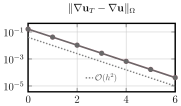
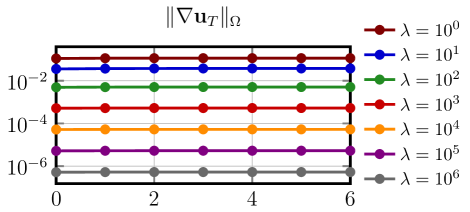
Figure 7. Discretizaton error for Example 1 (left) and norm of discrete error for Example 2 (right) for the method (S1), $k=2$, on a barycentric-refined mesh under mesh refinement ($x$-axis: refinement level $L$) and different values of $\lambda$ for Example 2.

4. Relaxed $H(\operatorname{\operatorname{div}})-$conforming HDG discretization

The results in Theorem 2 provide optimal error estimates for the method (S1). However, for the approximation of the displacement with a polynomial degree $k$ it requires unknowns of degree $k$ for the normal component of the displacement on every facet of the mesh. In view of the superconvergence property of other HDG methods [42, 14], where only unknowns of polynomial degree $k-1$ on the facets are required to obtain an accurate polynomial approximation of order $k$ (possibly after a local post-processing) this is sub-optimal. Here we follow [31] to slightly relax the $H(\operatorname{\operatorname{div}})$-conformity so that only unknowns of polynomial degree $k-1$ are involved for normal-continuity. This allows for optimality of the method also in the sense of superconvergent HDG methods. The resulting method is still volume-locking-free. We assume the polynomial degree $k\geq 2$ in the following discussion.

4.1. The relaxed $H(\operatorname{\operatorname{div}})$-conforming HDG scheme

We introduce the modified vector space

$$\boldsymbol{V}_{\!h}^{-}:= \;\{\boldsymbol{v}_{T}\in\prod_{T\in\mathcal{T}_{h}}[\mathbb{P}^{k}(T)]^{d}:\;\;\Pi_{F}^{k-1}[\![\boldsymbol{v}_{T}\cdot\boldsymbol{n}]\!]_{F}=0,\;\,\forall F\in\mathcal{F}_{h}\},$$ (32)

where $\Pi_{F}^{k-1}:L^{2}(F)\rightarrow P^{k-1}(F)$ is the $L^{2}(F)$-projection:

$$\int_{F}(\Pi_{F}^{k-1}w)v\,\mathrm{ds}=\int_{F}w\,v\,\mathrm{ds},\quad\forall v\in P^{k-1}(F).$$ (33)

Details of the construction of the finite element space $\boldsymbol{V}_{\!h}^{-}$ can be found in [31, Section 3]. Functions in $\boldsymbol{V}_{\!h}^{-}$ are only “almost normal-continuous”, but can be normal-discontinuous in the highest orders.

Denoting the compound finite element space

$$\underline{\boldsymbol{U}\!}_{h}^{\,-}:=\boldsymbol{V}_{\!h}^{-}\times M_{h},$$

then the relaxed $H(\operatorname{\operatorname{div}})$-conforming HDG scheme reads: Find $\underline{\boldsymbol{u}}_{h}\in\underline{\boldsymbol{U}\!}_{h}^{\,-}$ such that

$$a_{h}(\underline{\boldsymbol{u}}_{h},\underline{\boldsymbol{v}}_{h})=f(\underline{\boldsymbol{v}}_{h}),\quad\forall\underline{\boldsymbol{v}}_{h}\in\underline{\boldsymbol{U}\!}_{h}^{\,-}.$$ (S2)

Remark 5.

Notice that the globally coupled degrees of freedom for the above relaxed $H(\operatorname{\operatorname{div}})$-conforming scheme are polynomials of degree $k-1$ per facet for both tangential and normal component of the displacement, while that for the original $H(\operatorname{\operatorname{div}})$-conforming scheme (S1) are polynomials of degree $k-1$ per facet for the tangential component of the displacement, and polynomials of degree $k$ per facet for the normal component. This relaxation reduces the globally coupled degrees of freedom which improves the sparsity pattern of the linear systems.

4.2. Error estimates

The error analysis of the relaxed scheme (S2) follows closely from that for the original scheme (S1) in Theorem 2.

Due to the violation of $H(\operatorname{\operatorname{div}})$-conformity of $\boldsymbol{V}_{\!h}^{-}$, we have a consistency term to take care of.

Lemma 2.

Let $\boldsymbol{u}\in[H_{0}^{2}(\Omega)]^{d}$ be the solution to the equations (1) and define the splitting $\boldsymbol{f}=\boldsymbol{f}^{\mu}+\boldsymbol{f}^{\lambda}$ with $\boldsymbol{f}^{\mu}=-\operatorname{\operatorname{div}}\left(2\mu\nabla_{s}\boldsymbol{u}\right)$ and $\boldsymbol{f}^{\lambda}=-{\nabla}\left(\lambda\,\operatorname{\operatorname{div}}\boldsymbol{u}\right)$ and $f(\cdot)=f^{\mu}(\cdot)+f^{\lambda}(\cdot)$ correspondingly. Denote $\underline{\boldsymbol{u}}:=(\boldsymbol{u},\boldsymbol{u}^{t})\in\underline{\boldsymbol{U}\!}(h)$. There holds for all $\underline{\boldsymbol{v}}=(\boldsymbol{v}_{T},\boldsymbol{v}_{F})\in\underline{\boldsymbol{U}\!}_{h}^{\,-}+\underline{\boldsymbol{U}\!}(h)$

$$a_{h}^{\mu}(\underline{\boldsymbol{u}},\underline{\boldsymbol{v}}) =f^{\mu}(\underline{\boldsymbol{v}})+\mathcal{E}_{c}^{\mu}(\boldsymbol{u},\underline{\boldsymbol{v}}),$$ (34a)

$$a_{h}^{\lambda}(\underline{\boldsymbol{u}},\underline{\boldsymbol{v}}) =f^{\lambda}(\underline{\boldsymbol{v}})+\mathcal{E}_{c}^{\lambda}(\boldsymbol{u},\underline{\boldsymbol{v}}),$$ (34b)

$$a_{h}(\underline{\boldsymbol{u}},\underline{\boldsymbol{v}}) =f(\underline{\boldsymbol{v}})+\mathcal{E}_{c}(\boldsymbol{u},\underline{\boldsymbol{v}}),$$ (34c)

with

$$\mathcal{E}_{c}^{\mu}(\boldsymbol{u},\underline{\boldsymbol{v}}) =\sum_{T\in\mathcal{T}_{h}}\int_{\partial T}\left(2\mu(\nabla_{s}(\boldsymbol{u})\boldsymbol{n})\cdot\boldsymbol{n}\right)(id-\Pi_{F}^{k-1})(\boldsymbol{v}_{T}\cdot\boldsymbol{n}).$$ (34d)

$$\mathcal{E}_{c}^{\lambda}(\boldsymbol{u},\underline{\boldsymbol{v}}) =\sum_{T\in\mathcal{T}_{h}}\int_{\partial T}\left(\lambda\operatorname{\operatorname{div}}\boldsymbol{u}\right)(id-\Pi_{F}^{k-1})(\boldsymbol{v}_{T}\cdot\boldsymbol{n}),$$ (34e)

$$\mathcal{E}_{c}(\boldsymbol{u},\underline{\boldsymbol{v}}) =\mathcal{E}_{c}^{\mu}(\boldsymbol{u},\underline{\boldsymbol{v}})+\mathcal{E}_{c}^{\lambda}(\boldsymbol{u},\underline{\boldsymbol{v}}).$$ (34f)

Moreover, for $\boldsymbol{u}\in[H_{0}^{\ell}(\Omega)]^{d}$, $\ell\geq 2$ and $1\leq m\leq\min(k,\ell-1)$ we have

$$\mathcal{E}_{c}^{\mu}(\boldsymbol{u},\underline{\boldsymbol{v}}) \preceq h^{m}\mu^{1/2}\|\boldsymbol{u}\|_{m+1}\|\underline{\boldsymbol{v}}\|_{\mu,h},\quad\mathcal{E}_{c}^{\lambda}(\boldsymbol{u},\underline{\boldsymbol{v}})\preceq h^{m}\frac{\lambda}{\mu^{1/2}}\|\operatorname{\operatorname{div}}\boldsymbol{u}\|_{m}\|\underline{\boldsymbol{v}}\|_{\mu,h}.$$ (35a)

$$\mathcal{E}_{c}(\boldsymbol{u},\underline{\boldsymbol{v}}) \preceq h^{m}\left(\mu^{1/2}\|\boldsymbol{u}\|_{m+1}+\frac{\lambda}{\mu^{1/2}}\|\operatorname{\operatorname{div}}\boldsymbol{u}\|_{m}\right)\|\underline{\boldsymbol{v}}\|_{\mu,h}.$$ (35b)

Proof.

By continuity of $\boldsymbol{u}$ and integration by parts, we get

$$a_{h}^{\mu}(\underline{\boldsymbol{u}},\underline{\boldsymbol{v}})-f^{\mu}(\underline{\boldsymbol{v}})= \;\sum_{T\in\mathcal{T}_{h}}\int_{\partial T}2\mu\,\nabla_{s}(\boldsymbol{u})\boldsymbol{n}\cdot(\boldsymbol{v}_{T}-\boldsymbol{v}_{T}^{t})\,\mathrm{d}\boldsymbol{s}$$

$$= \;\sum_{T\in\mathcal{T}_{h}}\int_{\partial T}2\mu(\nabla_{s}(\boldsymbol{u})\boldsymbol{n}\cdot\boldsymbol{n}(\boldsymbol{v}_{T}\cdot\boldsymbol{n})\,\,\mathrm{d}\boldsymbol{s}$$

$$= \;\sum_{T\in\mathcal{T}_{h}}\int_{\partial T}(2\mu(\nabla_{s}(\boldsymbol{u})\boldsymbol{n})\cdot\boldsymbol{n})(id-\Pi_{F}^{k-1})(\boldsymbol{v}_{T}\cdot\boldsymbol{n})\,\,\mathrm{d}\boldsymbol{s}$$

$$= \;\mathcal{E}_{c}^{\mu}(\boldsymbol{u},\underline{\boldsymbol{v}}),$$

where the third equality follows from the fact that $\Pi_{F}^{k-1}[\![\boldsymbol{v}\cdot\boldsymbol{n}]\!]_{F}=0$ for all $\boldsymbol{v}\in\boldsymbol{V}_{\!h}^{-}$. Analogously we obtain $a_{h}^{\lambda}(\underline{\boldsymbol{u}},\underline{\boldsymbol{v}})-f^{\lambda}(\underline{\boldsymbol{v}})=\mathcal{E}_{c}^{\lambda}(\boldsymbol{u},\underline{\boldsymbol{v}})$.

Applying the Cauchy-Schwarz inequality and properties of the $L^{2}$-projection, we have

$$\mathcal{E}_{c}^{\mu}(\boldsymbol{u},\underline{\boldsymbol{v}})= \int_{\partial T}(id-\Pi_{F}^{k-1})\left(2\mu(\nabla_{s}(\boldsymbol{u})\boldsymbol{n})\cdot\boldsymbol{n}\right)(id-\Pi_{F}^{k-1})(\boldsymbol{v}_{T}\cdot\boldsymbol{n})$$

$$\;\leq\left(2\mu\|(id-\Pi_{F}^{k-1})\nabla_{s}(\boldsymbol{u})\|_{\partial T}\right)\|(id-\Pi_{F}^{k-1})(\boldsymbol{v}_{T}\cdot\boldsymbol{n})\|_{\partial T}$$

$$\;\preceq h^{m-1/2}\mu\|\nabla_{s}(\boldsymbol{u})\|_{H^{m}(T)}\|(id-\Pi_{F}^{k-1})(\boldsymbol{v}_{T}\cdot\boldsymbol{n})\|_{\partial T}$$

$$\;\preceq h^{m}\mu\|\boldsymbol{u}\|_{H^{m+1}(T)}\|(id-\Pi_{RM})\boldsymbol{v}_{T}\|_{\partial T}\;\preceq h^{m}\mu\|\boldsymbol{u}\|_{H^{m+1}(T)}\|\nabla_{s}\boldsymbol{v}_{T}\|_{T},$$

where the last inequality follows from the trace theorem and the approximation properties (18). Similarly,

$$\mathcal{E}_{c}^{\lambda}(\boldsymbol{u},\underline{\boldsymbol{v}})= \int_{\partial T}(id-\Pi_{F}^{k-1})\lambda\operatorname{\operatorname{div}}\boldsymbol{u}(id-\Pi_{F}^{k-1})(\boldsymbol{v}_{T}\cdot\boldsymbol{n})$$

$$\;\leq\lambda\|(id-\Pi_{F}^{k-1})\operatorname{\operatorname{div}}\boldsymbol{u}\|_{\partial T}\|(id-\Pi_{F}^{k-1})(\boldsymbol{v}_{T}\cdot\boldsymbol{n})\|_{\partial T}$$

$$\;\preceq h^{m}{\lambda}\|\operatorname{\operatorname{div}}\boldsymbol{u}\|_{H^{m}(T)}\|\nabla_{s}\boldsymbol{v}_{T}\|_{T}.$$

Summing over all elements concludes the proof. ∎

We have the following error estimates, whose proof follows closed from that for Theorem 2. We only sketch the proof with a focus on the modification needed from the proof for Theorem 2.

Theorem 4.

Assume $k\geq 2$ and the regularity $\boldsymbol{u}\in[H^{k+1}(\Omega)]^{d}$. Let $\underline{\boldsymbol{u}}_{h}\in\underline{\boldsymbol{U}\!}_{h}^{\,-}$ be the numerical solution to the scheme (S2). Then, for sufficiently large stabilization parameter $\alpha_{0}$, the following estimate holds

$$\|\underline{\boldsymbol{u}}-\underline{\boldsymbol{u}}_{h}\|_{\mu,h}\preceq \;h^{k}(\mu^{1/2}\|\boldsymbol{u}\|_{k+1}+\frac{\lambda}{\mu^{1/2}}\|\operatorname{\operatorname{div}}\boldsymbol{u}\|_{k}),$$ (36a)

$$\|\operatorname{\operatorname{div}}(\boldsymbol{u}-\boldsymbol{u}_{T})\|\preceq \;(\mu/\lambda)^{1/2}h^{k}\|\boldsymbol{u}\|_{k+1}+\left(\frac{\lambda^{1/2}}{\mu^{1/2}}+1\right)h^{k}\|\operatorname{\operatorname{div}}\,\boldsymbol{u}\|_{k}.$$ (36b)

Moreover, under the regularity assumption (20), the following estimate holds

$$\|\boldsymbol{u}-\boldsymbol{u}_{T}\|\preceq h^{k+1}\left(\|\boldsymbol{u}\|_{k+1}+(\frac{\lambda}{\mu}+1)\|\operatorname{\operatorname{div}}\boldsymbol{u}\|_{k}\right).$$ (36c)

Remark 6 (Volume-locking-free estimates).

For convex polygonal domain $\Omega$, it is proven [13] that

$$\mu\|\boldsymbol{u}\|_{2}+\lambda\|\operatorname{\operatorname{div}}\boldsymbol{u}\|_{1}\preceq\|\boldsymbol{f}\|.$$

If we have the regularity shift, for $k\geq 2$,

$$\mu\|\boldsymbol{u}\|_{k+1}+\lambda\|\operatorname{\operatorname{div}}\boldsymbol{u}\|_{k}\preceq\|\boldsymbol{f}\|_{k},$$

the above estimates are free of volume-locking when $\lambda\rightarrow+\infty$.

Proof.

To prove the energy estimates (36a) and (36b), we still take $\underline{\boldsymbol{v}}_{h}=(\Pi_{V}\boldsymbol{u},\Pi_{M}\boldsymbol{u})\in\underline{\boldsymbol{U}\!}_{h}\subset\underline{\boldsymbol{U}\!}_{h}^{\,-}$ as in the proof of Theorem 2. By coercivity,

$$\|\underline{\boldsymbol{u}}_{h}-\underline{\boldsymbol{v}}_{h}\|_{\mu,h}^{2}+\lambda\|\operatorname{\operatorname{div}}(\boldsymbol{u}_{T}-\boldsymbol{v}_{T})\|^{2}$$

$$\preceq a_{h}^{\mu}(\underline{\boldsymbol{u}}_{h}-\underline{\boldsymbol{v}}_{h},\underline{\boldsymbol{u}}_{h}-\underline{\boldsymbol{v}}_{h})+\lambda\|\operatorname{\operatorname{div}}(\boldsymbol{u}_{T}-\boldsymbol{v}_{T})\|^{2}$$

$$=a_{h}(\underline{\boldsymbol{u}}_{h}-\underline{\boldsymbol{v}}_{h},\underline{\boldsymbol{u}}_{h}-\underline{\boldsymbol{v}}_{h})=a_{h}(\underline{\boldsymbol{u}}-\underline{\boldsymbol{v}}_{h},\underline{\boldsymbol{u}}_{h}-\underline{\boldsymbol{v}}_{h})-\mathcal{E}_{c}(\boldsymbol{u},\underline{\boldsymbol{u}}_{h}-\underline{\boldsymbol{v}}_{h})$$

$$=a_{h}^{\mu}(\underline{\boldsymbol{u}}-\underline{\boldsymbol{v}}_{h},\;\underline{\boldsymbol{u}}_{h}-\underline{\boldsymbol{v}}_{h})-\mathcal{E}_{c}(\boldsymbol{u},\underline{\boldsymbol{u}}_{h}-\underline{\boldsymbol{v}}_{h})$$

$$\preceq\left(\|\underline{\boldsymbol{u}}-\underline{\boldsymbol{v}}_{h}\|_{\mu,\ast,h}+\mu^{1/2}h^{k}\|\boldsymbol{u}\|_{k+1}+\frac{\lambda}{\mu^{1/2}}h^{k}\|\operatorname{\operatorname{div}}\boldsymbol{u}\|_{k}\right)\|\underline{\boldsymbol{u}}_{h}-\underline{\boldsymbol{v}}_{h}\|_{\mu,h}$$

This implies

$$\|\underline{\boldsymbol{u}}-\underline{\boldsymbol{u}}_{h}\|_{\mu,h}+\lambda^{1/2}\|\operatorname{\operatorname{div}}(\boldsymbol{u}_{T}-\boldsymbol{v}_{T})\|\preceq h^{k}\left(\mu^{1/2}\|\boldsymbol{u}\|_{k+1}+\frac{\lambda}{\mu^{1/2}}\|\operatorname{\operatorname{div}}\boldsymbol{u}\|_{k}\right).$$

Then, the estimates (36a) and (36b) follows from (27) and the triangle inequality.

To prove the $L^{2}$-estimate, let $\boldsymbol{\phi}$ be the solution to the dual problem (21) with $\boldsymbol{\theta}=\boldsymbol{u}-\boldsymbol{u}_{T}$ and $\underline{\boldsymbol{\phi}}=(\boldsymbol{\phi},\boldsymbol{\phi}^{t})\in\underline{\boldsymbol{U}\!}(h)$. By symmetry of the bilinear form $a_{h}(\cdot,\cdot)$ and Lemma 2, we have, with $\underline{\boldsymbol{\phi}}_{h}=(\Pi_{V}\boldsymbol{\phi},\Pi_{M}\boldsymbol{\phi})\in\underline{\boldsymbol{U}\!}_{h}$

$$\|\boldsymbol{u}-\boldsymbol{u}_{T}\|_{\Omega}^{2} =a_{h}(\underline{\boldsymbol{\phi}},\underline{\boldsymbol{u}}-\underline{\boldsymbol{u}}_{h})-\mathcal{E}_{c}(\boldsymbol{\phi},\underline{\boldsymbol{u}}-\underline{\boldsymbol{u}}_{h})$$

$$=a_{h}(\underline{\boldsymbol{\phi}}-\underline{\boldsymbol{\phi}}_{h},\underline{\boldsymbol{u}}-\underline{\boldsymbol{u}}_{h})-\mathcal{E}_{c}(\boldsymbol{\phi},\underline{\boldsymbol{u}}-\underline{\boldsymbol{u}}_{h})+\underbrace{\mathcal{E}_{c}(\boldsymbol{u},\underline{\boldsymbol{\phi}}_{h})}_{=0}$$

$$\preceq h(\mu\|\boldsymbol{\phi}\|_{2}+\lambda\|\operatorname{\operatorname{div}}\boldsymbol{\phi}\|_{1})(\mu^{-1/2}\|\underline{\boldsymbol{u}}-\underline{\boldsymbol{u}}_{h}\|_{\mu,*,h}+\|(I-\Pi_{Q})\operatorname{\operatorname{div}}\boldsymbol{u}\|)$$

$$\preceq h^{k+1}\|\boldsymbol{u}-\boldsymbol{u}_{T}\|_{\Omega}\left(\|\boldsymbol{u}\|_{k+1}+(\frac{\lambda}{\mu}+1)\|\operatorname{\operatorname{div}}\boldsymbol{u}\|_{k}\right).$$

In the last step we invoked the regularity assumption (20). This completes the proof of (36c). ∎

Remark 7 (Lack of gradient-robustness as a locking phenomenon).

Although, the scheme (S2) is free of volume-locking, it is not free of another locking phenomenon, though. Indeed, the explicit dependence of the right side of the error estimate (36c) on $\lambda$ indicates a classical locking phenomenon in the sense of Babuška and Suri [8], where they write in the abstract: “A numerical scheme for the approximation of a parameter-dependent problem is said to exhibit locking if the accuracy of the approximations deteriorates as the parameter tends to a limiting value.” Comparing with the error estimate (22c) for the gradient-robust scheme (S1), we recognize that schemes for nearly-incompressible linear elasticity are only locking-free in the sense of [8], if they are gradient-robust and free of volume-locking, simultaneously. The situation is very similar to the incompressible Stokes problem. Only schemes, which are pressure-robust and discretely inf-sup stable simultaneously [1], are really locking-free in the sense of Babuška and Suri [8].

4.3. Numerical results for the scheme (S2)

The numerical results for the two examples in Section 2 for the scheme (S2) are given in Figure 8. We observe from Figure 8 (left) that the errors for the scheme (S2) are independent of $\lambda$ for Example 1, which are similar to those for the scheme (S1). This is consistent with the volume-locking-free estimates in Theorem 4. However, the norm of the discrete solution for the scheme (S2) for Example 2 shows an upper bound depending on $h$ which indicates that it is not gradient-robust. In the next subsection, we slightly modify the scheme (S2) to make it gradient-robust.

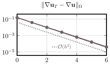
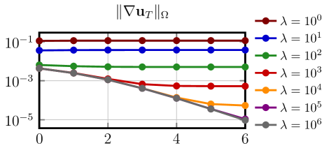
Figure 8. Discretizaton error for Example 1 (left) and norm of discrete error for Example 2 (right) for the method (S2), $k=2$, on a barycentric-refined mesh under mesh refinement ($x$-axis: refinement level $L$) and different values of $\lambda$ for Example 2.

4.4. Gradient-robust relaxed $H(\operatorname{\operatorname{div}})$-conforming HDG scheme

As in Section 3.5 we consider the equivalent DG formulation

$$\hat{a}_{h}(\boldsymbol{u}_{T},\boldsymbol{v}_{T})=\hat{f}(\boldsymbol{v}_{T})\quad\forall\boldsymbol{v}_{T}\in\boldsymbol{V}_{\!h}^{-},$$ (S2-DG)

If we consider a splitting as in (28) with

$$\boldsymbol{V}_{\!h}^{\,-,0}:=\{\boldsymbol{v}_{T}\in\boldsymbol{V}_{\!h}^{\,-}:\operatorname{\operatorname{div}}\boldsymbol{v}_{T}=0,\ \forall T\in\mathcal{T}_{h}\}$$ (37a)

and

$$\boldsymbol{V}_{\!h}^{\,-,\perp}:=\{\boldsymbol{v}_{T}\in\boldsymbol{V}_{\!h}^{\,-}:\hat{a}_{h}(\boldsymbol{v}_{T},\boldsymbol{w}_{T})=0,\forall\boldsymbol{w}_{T}\in\boldsymbol{V}_{\!h}^{\,-,0}\},$$ (37b)

we can again decompose every discrete function $\boldsymbol{v}_{T}\in\boldsymbol{V}_{\!h}^{\,-}$ as $\boldsymbol{v}_{T}=\boldsymbol{v}_{T}^{0}+\boldsymbol{v}_{T}^{\perp}$ with $\boldsymbol{v}_{T}^{0}\in\boldsymbol{V}_{\!h}^{\,-,0},\boldsymbol{v}_{T}^{\perp}\in\boldsymbol{V}_{\!h}^{\,-,\perp}$.

$$\hat{a}_{h}(\boldsymbol{u}_{T}^{0},\boldsymbol{v}_{T}^{0}) =\hat{f}(\boldsymbol{v}_{T}^{0})\quad\forall~{}\boldsymbol{v}_{T}^{0}\in\boldsymbol{V}_{\!h}^{\,-,0},$$ (38a)

$$\hat{a}_{h}(\boldsymbol{u}_{T}^{\perp},\boldsymbol{v}_{T}^{\perp}) =\hat{f}(\boldsymbol{v}_{T}^{\perp})\quad\forall~{}\boldsymbol{v}_{T}^{\perp}\in\boldsymbol{V}_{\!h}^{\,-,\perp}.$$ (38b)

Note that Theorem 3 does not directly translate to the relaxed $H(\operatorname{\operatorname{div}})$-conforming case only because (31) does not hold as the facet normal jumps do not vanish. However, we can introduce a modification in the treatment of the right hand side that re-enables gradient-robustness. The modified scheme is: Find $\underline{\boldsymbol{u}}_{h}\in\underline{\boldsymbol{U}\!}_{h}^{\,-}$ such that

$$a_{h}(\underline{\boldsymbol{u}}_{h},\underline{\boldsymbol{v}}_{h})=f((\Pi_{V}\boldsymbol{v}_{T},0)),\quad\forall\underline{\boldsymbol{v}}_{h}\in\underline{\boldsymbol{U}\!}_{h}^{\,-}.$$ (S3)

or in the equivalent DG formulation: Find $\boldsymbol{u}_{T}\in\boldsymbol{V}_{\!h}^{\,-}$ such that

$$\hat{a}_{h}(\boldsymbol{u}_{T},\boldsymbol{v}_{T})=\hat{f}(\Pi_{V}\boldsymbol{v}_{T}),\quad\forall\boldsymbol{v}_{T}\in\boldsymbol{V}_{\!h}^{\,-}.$$ (S3-DG)

Here, $\Pi_{V}$ is a generalization of the BDM interpolator, [10, Proposition 2.3.2], which can deal with only element-wise smooth functions by averaging, cf. the appendix for a definition.

Remark 8.

Let us note that the BDM interpolator is not mandatory here. In [31] and [32] several conditions on a suitable reconstruction operator are formulated. A much simpler version of the BDM interpolation operator is suggested that exploits the knowledge on the pre-image $\boldsymbol{V}_{\!h}^{\,-}$ and a proper basis for the relaxed $H(\operatorname{\operatorname{div}})$-conforming finite element space. The reconstruction operation can then be realized by a simple averaging of a few unknowns which makes it computationally very cheap. In the numerical examples below we make use of this operator.

Lemma 3.

The scheme (S3-DG) is gradient-robust, i.e. for $\boldsymbol{f}=\nabla\phi$, $\phi\in H^{1}(\Omega)$, the solution $\boldsymbol{u}_{T}=\boldsymbol{u}_{T}^{0}+\boldsymbol{u}_{T}^{\perp}\in\boldsymbol{V}_{\!h}^{\,-}$ has $\boldsymbol{u}_{T}^{0}=\boldsymbol{0},~{}\boldsymbol{u}_{T}^{\perp}=\mathcal{O}(\lambda^{-1}).$

Proof.

With $\hat{f}(\cdot)=(\nabla\phi,\Pi_{V}\cdot)_{\Omega}$ there holds after partial integration

$$\hat{f}(\boldsymbol{v}_{T}^{0})=-\sum_{T\in\mathcal{T}_{h}}(\phi,\operatorname{\operatorname{div}}\Pi_{V}\boldsymbol{v}^{0}_{T})_{T}+\sum_{F\in\mathcal{F}_{h}}(\phi,[\![\Pi_{V}\boldsymbol{v}^{0}_{T}\cdot\boldsymbol{n}]\!]_{F})=0~{}\forall~{}\boldsymbol{v}_{T}^{0}\in\boldsymbol{V}_{\!h}^{\,-,0}.$$ (39)

where we used $\operatorname{\operatorname{div}}\Pi_{V}\boldsymbol{v}^{0}_{T}=0$ cf. [31, Lemma 4.8] and $[\![\Pi_{V}\boldsymbol{v}^{0}_{T}\cdot\boldsymbol{n}]\!]_{F}=0$. The remainder of the proof follows from the proof of Theorem 3. ∎

For the robustness of the scheme we give the following improved version of Lemma 2 (in the DG setting).

Lemma 4.

Let $\boldsymbol{u}\in[H_{0}^{2}(\Omega)]^{d}$ be the solution to the equations (1) and define the splitting $\boldsymbol{f}=\boldsymbol{f}^{\mu}+\boldsymbol{f}^{\lambda}$ with $\boldsymbol{f}^{\mu}=-\operatorname{\operatorname{div}}\left(2\mu\nabla_{s}\boldsymbol{u}\right)$ and $\boldsymbol{f}^{\lambda}=-{\nabla}\left(\lambda\,\operatorname{\operatorname{div}}\boldsymbol{u}\right)$ and $f(\cdot)=f^{\mu}(\cdot)+f^{\lambda}(\cdot)$ and $\hat{f}(\cdot)=\hat{f}^{\mu}(\cdot)+\hat{f}^{\lambda}(\cdot)$ correspondingly. Denote $\underline{\boldsymbol{u}}:=(\boldsymbol{u},\boldsymbol{u}^{t})\in\underline{\boldsymbol{U}\!}(h)$. There holds for all $\underline{\boldsymbol{v}}=(\boldsymbol{v}_{T},\boldsymbol{v}_{F})\in\underline{\boldsymbol{U}\!}_{h}^{\,-}$

$$a_{h}^{\mu}(\underline{\boldsymbol{u}},\underline{\boldsymbol{v}}) =\hat{f}^{\mu}(\Pi_{V}\boldsymbol{v}_{T})+\widetilde{\mathcal{E}}_{c}^{\mu}(\boldsymbol{u},\underline{\boldsymbol{v}}),$$ (40a)

$$a_{h}^{\lambda}(\underline{\boldsymbol{u}},\underline{\boldsymbol{v}}) =\hat{f}^{\lambda}(\Pi_{V}\boldsymbol{v}_{T}),$$ (40b)

$$a_{h}(\underline{\boldsymbol{u}},\underline{\boldsymbol{v}}) =\hat{f}(\Pi_{V}\boldsymbol{v}_{T})+\widetilde{\mathcal{E}}_{c}^{\mu}(\boldsymbol{u},\underline{\boldsymbol{v}}),$$ (40c)

$$\text{with }\qquad\widetilde{\mathcal{E}}_{c}^{\mu}(\boldsymbol{u},\underline{\boldsymbol{v}}) =\mathcal{E}_{c}^{\mu}(\boldsymbol{u},\underline{\boldsymbol{v}})+\hat{f}^{\mu}(\boldsymbol{v}_{T}-\Pi_{V}\boldsymbol{v}_{T}).$$ (40d)

Moreover, for $\boldsymbol{u}\in[H_{0}^{\ell}(\Omega)]^{d}$, $\ell\geq 2$ and $1\leq m\leq\min(k,\ell-1)$ we have

$$\widetilde{\mathcal{E}}_{c}^{\mu}(\boldsymbol{u},\underline{\boldsymbol{v}}) \preceq h^{m}\mu^{1/2}\|\boldsymbol{u}\|_{m+1}\|\underline{\boldsymbol{v}}\|_{\mu,h}.$$ (41)

Proof.

From (34a) the result (40a) follows directly. Next, we note that $\operatorname{\operatorname{div}}\Pi_{V}\boldsymbol{v}_{T}=\operatorname{\operatorname{div}}\boldsymbol{v}_{T}$ for $\boldsymbol{v}_{T}\in\boldsymbol{V}_{\!h}^{-}$. This, we can see from the following observation. Let $q\in\mathbb{P}^{k-1}(T)$ and $T\in\mathcal{T}_{h}$. Then, we have

$$\int_{T}\operatorname{\operatorname{div}}(\Pi_{V}\boldsymbol{v}_{T})q\,dx =-\int_{T}\Pi_{V}\boldsymbol{v}_{T}\cdot\nabla q\,dx+\int_{\partial T}\Pi_{V}\boldsymbol{v}_{T}\cdot n\,q\,ds$$

$$=-\int_{T}\boldsymbol{v}_{T}\cdot\nabla q\,dx+\int_{\partial T}\boldsymbol{v}_{T}\cdot n\,q\,ds=\int_{T}\operatorname{\operatorname{div}}(\boldsymbol{v}_{T})q\,dx$$

where we exploited (43a) and (43b) of the BDM interpolation. As $\operatorname{\operatorname{div}}(\boldsymbol{v}_{T}),\operatorname{\operatorname{div}}(\Pi_{V}\boldsymbol{v}_{T})\in\mathbb{P}^{k-1}(T)$ we obtain $\operatorname{\operatorname{div}}(\boldsymbol{v}_{T})=\operatorname{\operatorname{div}}(\Pi_{V}\boldsymbol{v}_{T})$ pointwise. Then, (40b) follows from partial integration:

$$\hat{f}^{\lambda}(\Pi_{V}\boldsymbol{v}_{T}) =\sum_{T\in\mathcal{T}_{h}}\int_{T}-\nabla(\lambda\operatorname{\operatorname{div}}\boldsymbol{u})\Pi_{V}\boldsymbol{v}_{T}\,\mathrm{d}\boldsymbol{x}$$

$$=\sum_{T\in\mathcal{T}_{h}}\int_{T}\lambda\operatorname{\operatorname{div}}\boldsymbol{u}\underbrace{\operatorname{\operatorname{div}}(\Pi_{V}\boldsymbol{v}_{T})}_{=\operatorname{\operatorname{div}}\boldsymbol{v}_{T}}\,\mathrm{d}\boldsymbol{x}-\int_{\partial T}\lambda\operatorname{\operatorname{div}}\boldsymbol{u}\Pi_{V}\boldsymbol{v}_{T}\cdot\boldsymbol{n}\,\mathrm{d}\boldsymbol{s}$$

$$=a_{h}^{\lambda}(\underline{\boldsymbol{u}},\underline{\boldsymbol{v}})-\sum_{F\in\mathcal{F}_{h}\setminus\partial\Omega}\int_{F}\lambda\operatorname{\operatorname{div}}\boldsymbol{u}\underbrace{[\![\Pi_{V}\boldsymbol{v}_{T}]\!]_{\ast}}_{=0}\cdot\boldsymbol{n}\,\mathrm{d}\boldsymbol{s}=a_{h}^{\lambda}(\underline{\boldsymbol{u}},\underline{\boldsymbol{v}}).$$

Next, we note that for $T\in\mathcal{T}_{h}$ there holds with standard Bramble-Hilbert arguments ($\boldsymbol{v}_{T}\in H^{1}(T)$)

$$\|(\operatorname{\operatorname{id}}-\Pi_{V})\boldsymbol{v}_{T}\|_{T}^{2}\preceq h\|\nabla\boldsymbol{v}_{T}\|_{T}$$ (42)

as constants are in the kernel of $\operatorname{\operatorname{id}}-\Pi_{V}$. Let further $\mathcal{P}^{m-2}\boldsymbol{f}$ be the element-wise $L^{2}$ projection into $[\Pi^{m-2}(T)]^{d},~{}T\in\mathcal{T}_{h}$. Then, we have

$$(\boldsymbol{f}^{\mu}, \boldsymbol{v}_{T}-\Pi_{V}\boldsymbol{v}_{T})=(\boldsymbol{f}^{\mu}-\mathcal{P}^{m-2}\boldsymbol{f}^{\mu},\boldsymbol{v}_{T}-\Pi_{V}\boldsymbol{v}_{T})\leq\|\boldsymbol{f}^{\mu}-\mathcal{P}^{m-2}\boldsymbol{f}^{\mu}\|\|\boldsymbol{v}_{T}-\Pi_{V}\boldsymbol{v}_{T}\|$$

$$\preceq h^{m-1}\|\boldsymbol{f}^{\mu}\|_{m-1}~{}h\|\boldsymbol{v}_{T}\|_{1,h}\preceq h^{m}\mu\|\boldsymbol{u}\|_{m+1}~{}\|\underline{\boldsymbol{v}}\|_{1,h}\preceq h^{m}\mu^{\frac{1}{2}}\|\boldsymbol{u}\|_{m+1}~{}\|\underline{\boldsymbol{v}}\|_{\mu,h}.$$

Here, we made use of (43b) in the last step. ∎

Finally, the locking-free error estimates for the scheme (S3) is given below.

Theorem 5.

Assume $k\geq 2$ and the regularity $\boldsymbol{u}\in[H^{k+1}(\Omega)]^{d}$. Let $\boldsymbol{u}_{T}\in\boldsymbol{V}_{\!h}^{\,-}$ be the numerical solution to the scheme (S3-DG) (or equivalently $\underline{\boldsymbol{u}}_{h}=(\boldsymbol{u}_{T},\mathcal{L}_{h}(\boldsymbol{u}_{T}))\in\underline{\boldsymbol{U}\!}_{h}^{\,-}$ the numerical solution to (S3)). Then, for sufficiently large stabilization parameter $\alpha_{0}$, the estimates (22a)–(22c) hold.

Proof.

Proceeding as in the proof of Theorem 4 (and hence using the equivalent HDG-version again) with $\underline{\boldsymbol{v}}_{h}=(\Pi_{V}\boldsymbol{u},\Pi_{M}\boldsymbol{u})\in\underline{\boldsymbol{U}\!}_{h}\subset\underline{\boldsymbol{U}\!}_{h}^{\,-}$ and $\underline{\boldsymbol{w}}_{h}:=\underline{\boldsymbol{u}}_{h}-\underline{\boldsymbol{v}}_{h}\in\underline{\boldsymbol{U}\!}_{h}^{\,-}$, we obtain

$$\|\underline{\boldsymbol{w}}_{h}\|_{\mu,h}^{2}+\lambda\|\operatorname{\operatorname{div}}(\boldsymbol{w}_{T})\|^{2}$$

$$\preceq a_{h}(\underline{\boldsymbol{w}}_{h},\underline{\boldsymbol{w}}_{h})=a_{h}(\underline{\boldsymbol{u}}-\underline{\boldsymbol{v}}_{h},\underline{\boldsymbol{w}}_{h})-\widetilde{\mathcal{E}}_{c}^{\mu}(\boldsymbol{u},\underline{\boldsymbol{w}}_{h})$$

$$=a_{h}^{\mu}(\underline{\boldsymbol{u}}-\underline{\boldsymbol{v}}_{h},\;\underline{\boldsymbol{w}}_{h})+\underbrace{a_{h}^{\lambda}(\underline{\boldsymbol{u}}-\underline{\boldsymbol{v}}_{h},\;\underline{\boldsymbol{w}}_{h})}_{=0}-\widetilde{\mathcal{E}}_{c}^{\mu}(\boldsymbol{u},\underline{\boldsymbol{w}}_{h})$$

$$\preceq\left(\|\underline{\boldsymbol{u}}-\underline{\boldsymbol{v}}_{h}\|_{\mu,\ast,h}+\mu^{\frac{1}{2}}h^{k}\|\boldsymbol{u}\|_{k+1}\right)\|\underline{\boldsymbol{w}}_{h}\|_{\mu,h}.$$

With interpolation estimates for $\|\underline{\boldsymbol{u}}-\underline{\boldsymbol{v}}_{h}\|_{\mu,\ast,h}$ this implies

$$\|\underline{\boldsymbol{u}}_{h}-\underline{\boldsymbol{v}}_{h}\|_{\mu,h}+\lambda^{\frac{1}{2}}\|\operatorname{\operatorname{div}}(\boldsymbol{u}_{T}-\boldsymbol{v}_{T})\|\preceq\mu^{\frac{1}{2}}h^{k}\|\boldsymbol{u}\|_{k+1}.$$

Then, the estimates (22a) and (22b) follow from triangle inequalities.

For the $L^{2}$-estimate, let $\boldsymbol{\phi}$ be the solution to the dual problem (21) with $\boldsymbol{\theta}=\Pi_{V}(\boldsymbol{u}-\boldsymbol{u}_{T})$ and $\underline{\boldsymbol{\phi}}_{h}\in\underline{\boldsymbol{U}\!}_{h}$ the corresponding interpolation as before. Noting that $\widetilde{\mathcal{E}}_{c}^{\mu}(\cdot,\underline{\boldsymbol{w}}_{h})$ does not depend on $\boldsymbol{w}_{F}=\boldsymbol{u}_{F}-\Pi_{M}\boldsymbol{u}$, cf. Lemma 2 and Lemma 4, and $\underline{\boldsymbol{\phi}}=(\boldsymbol{\phi},\boldsymbol{\phi}^{t})$ we get for $\Pi\underline{\boldsymbol{v}}=\Pi(\boldsymbol{v}_{T},\boldsymbol{v}_{F})=(\Pi_{V}\boldsymbol{v}_{T},\Pi_{M}\boldsymbol{v}_{F})$, $\underline{\boldsymbol{v}}=(\boldsymbol{v}_{T},\boldsymbol{v}_{F})\in\underline{\boldsymbol{U}\!}(h)$

$$\|\Pi_{V}(\boldsymbol{u}-\boldsymbol{u}_{T})\|_{\Omega}^{2} =a_{h}(\underline{\boldsymbol{\phi}},\Pi(\underline{\boldsymbol{u}}-\underline{\boldsymbol{u}}_{h}))-\overbrace{\widetilde{\mathcal{E}}_{c}^{\mu}(\boldsymbol{\phi},\Pi(\underline{\boldsymbol{u}}-\underline{\boldsymbol{u}}_{h}))}^{=0}$$

$$=a_{h}(\underline{\boldsymbol{\phi}},\underline{\boldsymbol{u}}-\underline{\boldsymbol{u}}_{h})-a_{h}(\underline{\boldsymbol{\phi}},(\operatorname{\operatorname{id}}-\Pi)(\underline{\boldsymbol{u}}-\underline{\boldsymbol{u}}_{h}))$$

$$=a_{h}(\underline{\boldsymbol{\phi}}-\underline{\boldsymbol{\phi}}_{h},\underline{\boldsymbol{u}}-\underline{\boldsymbol{u}}_{h})-a_{h}(\underline{\boldsymbol{\phi}},(\operatorname{\operatorname{id}}-\Pi)(\underline{\boldsymbol{u}}-\underline{\boldsymbol{u}}_{h}))+\overbrace{\widetilde{\mathcal{E}}^{\mu}_{c}(\boldsymbol{u},\underline{\boldsymbol{\phi}}_{h})}^{=0}$$

$$=a_{h}(\underline{\boldsymbol{\phi}}-\underline{\boldsymbol{\phi}}_{h},\underline{\boldsymbol{u}}-\underline{\boldsymbol{u}}_{h})-\underbrace{(\boldsymbol{\theta},(\operatorname{\operatorname{id}}-\Pi_{V})(\boldsymbol{u}-\boldsymbol{u}_{T}))}_{(\Pi_{V}(\boldsymbol{u}-\boldsymbol{u}_{T}),(\operatorname{\operatorname{id}}-\Pi_{V})(\boldsymbol{u}-\boldsymbol{u}_{T}))=0}$$

$$\preceq h(\mu\|\boldsymbol{\phi}\|_{2}+\lambda\|\operatorname{\operatorname{div}}\boldsymbol{\phi}\|_{1})(\mu^{-\tfrac{1}{2}}\|\underline{\boldsymbol{u}}-\underline{\boldsymbol{u}}_{h}\|_{\mu,\ast,h}+\|(\operatorname{\operatorname{id}}-\Pi_{Q})\operatorname{\operatorname{div}}\boldsymbol{u}_{T}\|)$$

$$\preceq\|\Pi_{V}(\boldsymbol{u}-\boldsymbol{u}_{T})\|_{\Omega}\cdot\left(h\left(\mu^{-\tfrac{1}{2}}\|\underline{\boldsymbol{u}}-\underline{\boldsymbol{u}}_{h}\|_{\mu,\ast,h}+\|(\operatorname{\operatorname{id}}-\Pi_{Q})\operatorname{\operatorname{div}}\boldsymbol{u}\|\right)\right)$$

Dividing by $\|\Pi_{V}(\boldsymbol{u}-\boldsymbol{u}_{T})\|_{\Omega}$ and applying the triangle inequality:

$$\|\boldsymbol{u}-\boldsymbol{u}_{T}\|_{\Omega}\leq\|\Pi_{V}(\boldsymbol{u}-\boldsymbol{u}_{T})\|_{\Omega}+\underbrace{\|(\operatorname{\operatorname{id}}-\Pi_{V})(\boldsymbol{u}-\boldsymbol{u}_{T})\|_{\Omega}}_{\preceq h\|\underline{\boldsymbol{u}}-\underline{\boldsymbol{u}}_{h}\|_{1,h}}$$

yields

$$\|\boldsymbol{u}-\boldsymbol{u}_{T}\|_{\Omega}\preceq h\left(\mu^{-\tfrac{1}{2}}\|\underline{\boldsymbol{u}}-\underline{\boldsymbol{u}}_{h}\|_{\mu,\ast,h}+\|(\operatorname{\operatorname{id}}-\Pi_{Q})\operatorname{\operatorname{div}}\boldsymbol{u}\|\right)$$

and hence the claim. ∎

With this result we conclude that method (S3) has quasi-optimal a-priori error bounds and is free of locking, i.e. it is volume-locking free and gradient-robust.

4.5. Numerical results for the scheme (S3)

The numerical results for the two examples in Section 2 for the scheme (S3) are given in Figure 9. The results are essentially similar to those for the scheme (S1). In particular, we observe that the discrete norms in Example 2 are essentially independent of $h$.

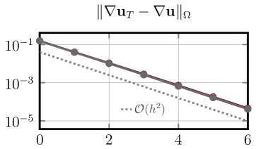
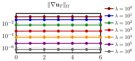
Figure 9. Discretizaton error for Example 1 (left) and norm of discrete error for Example 2 (right) for the method (S3), $k=2$, on a barycentric-refined mesh under mesh refinement ($x$-axis: refinement level $L$) and different values of $\lambda$ for Example 2.

5. Conclusion

The concept of gradient-robustness for numerical methods for linear elasticity is introduced in this paper. The class of divergence-conforming HDG methods are presented and analyzed as an example of volume-locking-free and gradient-robust finite element methods for linear elasticity. Two efficient variants of the base divergece-conforming HDG scheme with reduced globally coupled degrees of freedom are also discussed and analyzed.

Appendix. The BDM interpolator for discontinuous functions

The BDM interpolator for discontinuous functions is defined element-by-element for $\boldsymbol{v}_{T}\in H^{1}(T)$ through

$$(\Pi_{V}\boldsymbol{v}_{T}\!\cdot\!\boldsymbol{n},\varphi)_{F} =(\{\!\!\{\boldsymbol{v}_{T}\!\cdot\!\boldsymbol{n}\}\!\!\}_{*},\varphi)_{F} \forall~{}\varphi\!\in\!\mathcal{P}^{k}\!(F),F\!\in\!\partial T,$$ (43a)

$$(\Pi_{V}\boldsymbol{v}_{T},\varphi)_{T} =(\boldsymbol{v}_{T},\varphi)_{T} \forall~{}\varphi\in[\mathcal{N}^{k-2}(T)]^{d},$$ (43b)

with $\mathcal{N}^{k-2}:=[\mathcal{P}^{k-2}(T)]^{d}+[\mathcal{P}^{k-2}(T)]^{d}\times x$ and $\{\!\!\{\cdot\}\!\!\}_{*}$ the usual DG average operator, cf. [15, 24].

References

- [1] N. Ahmed, A. Linke, and C. Merdon, On really locking-free mixed finite element methods for the transient incompressible Stokes equations, SIAM J. Numer. Anal., 56 (2018), pp. 185–209.
- [2] M. Akbas, T. Gallouet, A. Gassmann, A. Linke, and C. Merdon, A gradient-robust well-balanced scheme for the compressible isothermal stokes problem, 2019.
- [3] D. N. Arnold, F. Brezzi, and J. Douglas, Jr., PEERS: a new mixed finite element for plane elasticity, Japan J. Appl. Math., 1 (1984), pp. 347–367.
- [4] D. N. Arnold, J. Douglas, Jr., and C. P. Gupta, A family of higher order mixed finite element methods for plane elasticity, Numer. Math., 45 (1984), pp. 1–22.
- [5] D. N. Arnold, R. S. Falk, and R. Winther, Mixed finite element methods for linear elasticity with weakly imposed symmetry, Math. Comp., 76 (2007), pp. 1699–1723.
- [6] D. N. Arnold and R. Winther, Mixed finite elements for elasticity, Numer. Math., 92 (2002), pp. 401–419.
- [7] D. N. Arnold and R. Winther, Nonconforming mixed elements for elasticity, Math. Models Methods Appl. Sci., 13 (2003), pp. 295–307. Dedicated to Jim Douglas, Jr. on the occasion of his 75th birthday.
- [8] I. Babuška and M. Suri, Locking effects in the finite element approximation of elasticity problems, Numer. Math., 62 (1992), pp. 439–463.
- [9] L. Beirão da Veiga, F. Brezzi, and L. D. Marini, Virtual elements for linear elasticity problems, SIAM J. Numer. Anal., 51 (2013), pp. 794–812.
- [10] D. Boffi, F. Brezzi, and M. Fortin, Mixed finite element methods and applications, vol. 44 of Springer Series in Computational Mathematics, Springer, Heidelberg, 2013.
- [11] D. Braess, Finite Elemente: Theorie, schnelle Löser und Anwendungen in der Elastizitätstheorie, Springer-Verlag, 2013.
- [12] S. C. Brenner, Korn’s inequalities for piecewise vector fields, Math. Comp., 73 (2004), pp. 1067–1087.
- [13] S. C. Brenner and L.-Y. Sung, Linear finite element methods for planar linear elasticity, Math. Comp., 59 (1992), pp. 321–338.
- [14] B. Cockburn and G. Fu, Devising superconvergent HDG methods with symmetric approximate stresses for linear elasticity by -decompositions, IMA J. Numer. Anal., 38 (2018), pp. 566–604.
- [15] B. Cockburn, G. Kanschat, and D. Schotzau, A locally conservative LDG method for the incompressible Navier-Stokes equations, Math. Comp., 74 (2005), pp. 1067–1095 (electronic).
- [16] B. Cockburn, D. Schötzau, and J. Wang, Discontinuous Galerkin methods for incompressible elastic materials, Comput. Methods Appl. Mech. Engrg., 195 (2006), pp. 3184–3204.
- [17] B. Cockburn and K. Shi, Superconvergent HDG methods for linear elasticity with weakly symmetric stresses, IMA J. Numer. Anal., 33 (2013), pp. 747–770.
- [18] D. A. Di Pietro and A. Ern, A hybrid high-order locking-free method for linear elasticity on general meshes, Comput. Methods Appl. Mech. Engrg., 283 (2015), pp. 1–21.
- [19] R. S. Falk, Nonconforming finite element methods for the equations of linear elasticity, Math. Comp., 57 (1991), pp. 529–550.
- [20] G. Fu and C. Lehrenfeld, A strongly conservative hybrid DG/mixed FEM for the coupling of Stokes and Darcy flow, Journal of Scientific Computing, 77, pp. 1605–1620.
- [21] N. R. Gauger, A. Linke, and P. W. Schroeder, On high-order pressure-robust space discretisations, their advantages for incompressible high Reynolds number generalised Beltrami flows and beyond, SMAI J. Comput. Math., 5 (2019), pp. 89–129.
- [22] J. Gopalakrishnan and J. Guzmán, Symmetric nonconforming mixed finite elements for linear elasticity, SIAM J. Numer. Anal., 49 (2011), pp. 1504–1520.
- [23] J. Guzmán and M. Neilan, Symmetric and conforming mixed finite elements for plane elasticity using rational bubble functions, Numer. Math., 126 (2014), pp. 153–171.
- [24] J. Guzmán, C.-W. Shu, and F. A. Sequeira, H (div) conforming and dg methods for incompressible euler’s equations, IMA Journal of Numerical Analysis, (2016), p. drw054.
- [25] P. Hansbo and M. G. Larson, Discontinuous Galerkin methods for incompressible and nearly incompressible elasticity by Nitsche’s method, Comput. Methods Appl. Mech. Engrg., 191 (2002), pp. 1895–1908.
- [26] P. Haupt, Continuum Mechanics and Theory of Materials, Springer Berlin, 2 ed., 2002.
- [27] S. Jin, Efficient asymptotic-preserving (AP) schemes for some multiscale kinetic equations, SIAM J. Sci. Comput., 21 (1999), pp. 441–454.
- [28] V. John, Finite element methods for incompressible flow problems, Springer, 2016.
- [29] V. John, A. Linke, C. Merdon, M. Neilan, and L. G. Rebholz, On the divergence constraint in mixed finite element methods for incompressible flows, SIAM Rev., 59 (2017), pp. 492–544.
- [30] H. T. J.R., M. Cohen, and M. Haroun, Reduced and selective integration techniques in the finite element analysis of plates, Nuclear Engineering and Design, 46 (1978), pp. 203–222.
- [31] P. L. Lederer, C. Lehrenfeld, and J. Schöberl, Hybrid discontinuous galerkin methods with relaxed h(div)-conformity for incompressible flows. part i, arXiv preprint arXiv:1707.02782, (2017).
- [32] , Hybrid discontinuous Galerkin methods with relaxed H(div)-conformity for incompressible flows. part ii, arXiv preprint arXiv:1805.06787, (2018).
- [33] P. L. Lederer and J. Schöberl, Polynomial robust stability analysis for (div)-conforming finite elements for the stokes equations, IMA Journal of Numerical Analysis, (2017).
- [34] C. Lehrenfeld, Hybrid Discontinuous Galerkin methods for solving incompressible flow problems, 2010. Diploma Thesis, MathCCES/IGPM, RWTH Aachen.
- [35] C. Lehrenfeld and J. Schöberl, High order exactly divergence-free hybrid discontinuous galerkin methods for unsteady incompressible flows, Computer Methods in Applied Mechanics and Engineering, 307 (2016), pp. 339–361.
- [36] A. Linke, On the role of the Helmholtz decomposition in mixed methods for incompressible flows and a new variational crime, Comput. Methods Appl. Mech. Engrg., 268 (2014), pp. 782–800.
- [37] A. Linke and C. Merdon, On velocity errors due to irrotational forces in the Navier-Stokes momentum balance, J. Comput. Phys., 313 (2016), pp. 654–661.
- [38] , Pressure-robustness and discrete Helmholtz projectors in mixed finite element methods for the incompressible Navier-Stokes equations, Comput. Methods Appl. Mech. Engrg., 311 (2016), pp. 304–326.
- [39] D. S. Malkus and H. T. J.R., Mixed finite element methods — reduced and selective integration techniques: A unification of concepts, Comput. Methods Appl. Mech. Engrg., 15 (1978), pp. 63–81.
- [40] M. A. Olshanskii and L. G. Rebholz, Application of barycenter refined meshes in linear elasticity and incompressible fluid dynamics, Electron. Trans. Numer. Anal., 38 (2011), pp. 258–274.
- [41] A. Pechstein and J. Schöberl, Tangential-displacement and normal-normal-stress continuous mixed finite elements for elasticity, Math. Models Methods Appl. Sci., 21 (2011), pp. 1761–1782.
- [42] W. Qiu, J. Shen, and K. Shi, An HDG method for linear elasticity with strong symmetric stresses, Math. Comp., 87 (2018), pp. 69–93.
- [43] W. Qiu and K. Shi, An HDG Method for Convection Diffusion Equation, J. Sci. Comput., 66 (2016), pp. 346–357.
- [44] L. R. Scott and M. Vogelius, Norm estimates for a maximal right inverse of the divergence operator in spaces of piecewise polynomials, RAIRO Modél. Math. Anal. Numér., 19 (1985), pp. 111–143.
- [45] S.-C. Soon, B. Cockburn, and H. Stolarski, A hybridizable discontinuous Galerkin method for linear elasticity, Internat. J. Numer. Methods Engrg., 80 (2009), pp. 1058–1092.
- [46] M. Vogelius, An analysis of the -version of the finite element method for nearly incompressible materials. Uniformly valid, optimal error estimates, Numer. Math., 41 (1983), pp. 39–53.
- [47] O. C. Zienkiewics, R. L. Taylor, and J. M. Too, Reduced integration techniques in general analysis of plates and shells, Internat. J. Numer. Meth. Engng., 5 (1971), pp. 275–290.