Collisional time and shear relaxation time for interacting QGP

We have estimated two different time scales of interacting quark gluon plasma (QGP) system. One is collisional time scale $\tau_{c}$, which carry microscopic interaction of quarks and gluons in medium. Another is shear relaxation time $\tau$, tuning the strength of shear viscosity coefficients QGP. Following the comments of Ref. Muronga , two time scales are different but no general formula linking $\tau$ and $\tau_{c}$ exists; their relationship depends in each case on the system under consideration. The present work has attempted to estimate these two time scales for interacting QGP and to realize their comparative strengths.

Let us first estimate the $\tau_{c}=1/\Gamma_{c}$, where $\Gamma_{c}$ is thermal width of quarks or gluons. We can understand the transition from non-interacting to interacting picture of QGP system as transition from $\Gamma_{c}=0$ to $\Gamma_{c}\neq 0$. It provides a possibility to map interaction of QGP by introducing a finite thermal width of quarks and gluons. This well-standard technique can be found in Ref. Cassing and references therein.

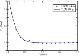
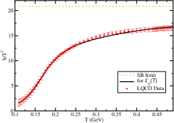
Figure 1: (a) Temperature dependence thermal width $\Gamma_{c}(T)$ parametrization curve (solid line) and LQCD extracted points (stars). (b) Their corresponding $s/T^{3}$ plots, where straight horizontal dotted line indicates SB limits of $s/T^{3}$.

Using spectral function $\rho(M,m_{i})$ of quarks and gluons for finite $\Gamma_{c}$ in interacting picture, we can express entropy density as

$$s = \sum_{i=u,d,s,g}g_{i}\int_{0}^{\infty}dM\rho(M,m_{i})\int_{0}^{\infty}\frac{d^{3}p}{(2\pi)^{3}}$$ (1)

$$\Big{(}\sqrt{p^{2}+M^{2}}+\frac{p^{2}}{3\sqrt{p^{2}+M^{2}}}\Big{)}$$

$$\frac{1}{{\rm exp}(\beta\sqrt{p^{2}+M^{2}})-a_{i}}~{},$$

where $a_{i}=\pm 1$ for fermion ($u$, $d$, $s$ quarks), boson (gluon $g$) respectively, and the spectral functions of constituents of non-interacting and interacting medium are respectively

$$\rho(M,m_{i}) = \delta(M-m_{i})$$

$$\rho(M,m_{i}) = \frac{1}{\pi}\Big{(}\frac{\Gamma_{c}}{\Gamma_{c}^{2}+(M-m_{i})^{2}}\Big{)}~{},$$ (2)

where $M$, $m_{i}$ is off-shell, on-shell mass of constituents. One can get back delta distribution for vanishing thermal width because of relation

$$\delta(M-M_{i})=\lim_{\Gamma_{c}\rightarrow 0}\rho(M,m_{i})~{}.$$ (3)

Hence, in non-interacting picture ($\Gamma_{c}\rightarrow 0$) as well as massless limit, Eq. (1) merges to standard Stephan-Boltzmann (SB) limiting value:

$$s=\Big{[}g_{g}+(g_{u}+g_{s})\Big{(}\frac{7}{8}\Big{)}\Big{]}\frac{4\pi^{2}}{90}T^{3}\approx 20.8~{}T^{3}~{}.$$ (4)

According to lattice Quantum Chromo Dynamics (LQCD) calculation LQCD1 , the numerical values of $s$ for QGP remain always lower than its SB limits. It can be seen from Fig. 1(b). By tuning $\Gamma_{c}$ in Eq. (1), we have match LQCD data LQCD1 , where we get parametrized of $\Gamma_{c}(T)$:

$$\Gamma_{c}(T)=a_{0}-\frac{a_{1}}{e^{a_{2}(T-a_{3})}+a_{4}}$$ (5)

with $a_{0}=6.76802$, $a_{1}=88.6265$, $a_{2}=-37.3715$, $a_{3}=0.170$, $a_{4}=14.0653$. It is plotted in Fig. 1(a).

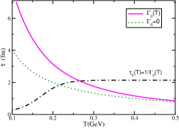
Figure 2: By imposing $\eta/s=1/(4\pi)$, $\tau(T)$ has been found for non-interacting or $\Gamma_{c}=0$ (dotted line) and interacting or $\Gamma_{c}(T)$ (solid line) cases. The $\tau_{c}(T)=1/\Gamma_{c}(T)$ is also plotted to compare with relaxation time scale $\tau$.

Now let us focus on other time scale - shear relaxation time $\tau$, which basically tune the shear viscosity expression

$$\eta = \tau\sum_{i=u,d,s,g}g_{i}\int_{0}^{\infty}dM\rho(M,m_{i})\int_{0}^{\infty}\frac{d^{3}p}{(2\pi)^{3}}$$ (6)

$$\Big{(}\frac{p^{4}}{p^{2}+M^{2}}\Big{)}\frac{{\rm exp}(\beta\sqrt{p^{2}+M^{2}})}{{\rm exp}(\beta\sqrt{p^{2}+M^{2}})-a_{i}}~{},$$

The $\tau$ in $\eta$ can be guessed from experimental data of QGP fluid, which indicates about its perfect fluid nature i.e. $\eta/s$ touch the KSS value $1/(4\pi)$. So imposing $\eta/s=1/(4\pi)$ for non-interacting and interacting picture, based on $\Gamma_{c}(T)$ parametrization, we have generated dotted and solid lines respectively in Fig. 2. Now, drawing collisional time $\tau_{c}=1/\Gamma_{c}$ by dash-dotted line in Fig. 2, we can get a pictorial knowledge of $\tau$ and $\tau_{c}$ in one frame. In kinetic theory approximation, we generally consider $\tau\approx\tau_{c}$, which might be more or less applicable near and above transition temperature at least in order of magnitude ($\tau_{c}\approx 2$ fm, $\tau\approx 1$ fm). It indicates that high temperature QCD interaction time scale, covered by LQCD data is quite well agreement with shear dissipative interaction of QGP. A detail investigation on it can be seen in Ref. LQCD_QGP .

References

- (1) A. Muronga, Causal theories of dissipative relativistic fluid dynamics for nuclear collisions Phys. Rev. C 69, 034903 (2004)
- (2) W. Cassing, QCD thermodynamics and confinement from a dynamical quasi-particle point of view Nucl. Phys. A 791 (2007) 365.
- (3) S. Borsanyi et. al., Full result for the QCD equation of state with 2+1 flavors, Phys. Lett. B 370 (2014) 99, arXiv:1309.5258 [hep-lat].
- (4) S. Satapathy, S. Paul, A. Anand, R. Kumar, S. Ghosh, From Non-interacting to Interacting Picture of Thermodynamics and Transport Coefficients for Quark Gluon Plasma, arXiv:1908.04330 [hep-ph]