Optimal by Design: Model-Driven Synthesis of Adaptation Strategies for Autonomous Systems

Abstract

Many software systems have become too large and complex to be managed efficiently by human administrators, particularly when they operate in uncertain and dynamic environments and require frequent changes. Requirements-driven adaptation techniques have been proposed to endow systems with the necessary means to autonomously decide ways to satisfy their requirements. However, many current approaches rely on general-purpose languages, models and/or frameworks to design, develop and analyze autonomous systems. Unfortunately, these tools are not tailored towards the characteristics of adaptation problems in autonomous systems. In this paper, we present Optimal by Design (ObD ), a framework for model-based requirements-driven synthesis of optimal adaptation strategies for autonomous systems. ObD  proposes a model (and a language) for the high-level description of the basic elements of self-adaptive systems, namely the system, capabilities, requirements and environment. Based on those elements, a Markov Decision Process (MDP) is constructed to compute the optimal strategy or the most rewarding system behavior. Furthermore, this defines a reflex controller that can ensure timely responses to changes. One novel feature of the framework is that it benefits both from goal-oriented techniques, developed for requirement elicitation, refinement and analysis, and synthesis capabilities and extensive research around MDPs, their extensions and tools. Our preliminary evaluation results demonstrate the practicality and advantages of the framework.

I Introduction

Autonomous systems such as unmanned vehicles and robots play an increasingly relevant role in our societies. Many factors contribute to the complexity in the design and development of those systems. First, they typically operate in dynamic and uncontrollable environments [1, 2, 3, 4, 5]. Therefore, they must continuously adapt their configuration in response to changes, both in their operating environment and in themselves. Since the frequency of change cannot be controlled, decision-making must be almost instantaneous to ensure timely responses. From a design and management perspective, it is desirable to minimize the effort needed to design the system and to enable its runtime updating and maintenance.

A promising technique to address those challenges is requirements-driven adaptation that endow systems with the necessary means to autonomously operate based on their requirements. Requirements are prescriptive statements of intent to be satisfied by cooperation of the agents forming the system [6]. They say what the system will do and not how it will do it [7]. Hence, software engineers are relieved from the onerous task of prescribing explicitly how to adapt the system when changes occur. Many current requirements-driven adaptation techniques [8, 9] follow the Monitor-Analyze-Plan-Execute-Knowledge (MAPE-K) paradigm [10], which usually works as follows [11]: the Monitor monitors the managed system and its environment, and updates the content of the Knowledge element accordingly; the Analyse activity uses the up-to-date knowledge to determine whether there is a need for adaptation of the managed element according to the adaptation goals that are available in the knowledge element. If adaptation is required, the Plan activity puts together a plan that consists of one or more adaptation actions. The adaptation plan is then executed by the Execute phase.

This approach has two main limitations in highly-dynamic operational environments. First, it tends to be myopic since the system adapts in response to changes without anticipating what the subsequent adaptation needs will be [5] and, thus, it does not guarantee the optimality of the overall behavior of the autonomous system. This is particularly crucial for systems that have to operate continuously without interruption over long periods of time, e.g., cyber-physical systems. Second, the time to plan adaptations could make timely reaction to changes impossible, particularly in fast changing environments. Therefore, an approach that enables an almost instantaneous reactions to changes is needed.

In this paper, we propose the Optimal by Design (ObD ) framework as a first step towards dealing with the aforementioned challenges. ObD supports a model-based approach to simplify the high-level design and description of autonomous systems, their capabilities, requirements and environment. Based on these high-level models, ObD constructs a Markov Decision Process (MDP) that can then be solved (possibly using state-of-the-art probabilistic model checkers) to produce optimal strategies for the autonomous system. These strategies define optimal reflex controllers that ensure the ability of autonomous systems to behave optimally and almost instantaneously to changes in itself or its environment.

Several previous works [12, 13, 5, 14] encode adaptation problems using general-purpose languages such as those proposed by probabilistic model checkers, e.g., PRISM [15]. Unfortunately, these languages do not offer primitives tailored to the design and analysis of autonomous systems. This makes them unsuitable to adequately describe the software requirements [6] of the autonomous system and the environment in which it operates. Examples of limitations of these languages resolved in this paper through ObD are the Markovian assumption [16] and the implicit-event model [17].

In a nutshell, ObD introduces a novel Domain Specific Modeling Language (DSL) for the description of autonomous systems, its environment and requirements. The semantics of the DSL is then defined in terms of a translation into a Markov Decision Process (MDP) model to enable the synthesis of optimal controllers for the autonomous system. This separation between the model (i.e. the DSL) and its underlying computational paradigm (i.e. MDP), brings several important advantages. First, the level of abstraction at which systems have to be designed is raised, simplifying their modeling by software engineers. Second, requirements become first-class entities, making it possible to elicit them using traditional requirements engineering techniques [6, 18, 19, 20] and to benefit from goal refinement, analysis and verification techniques developed for goal modeling languages. Moreover, this approach clarifies the limitations of the underlying computational model, namely the aforementioned Markovian assumption and the implicit-event model, and permits the identification and implementation of extensions necessary to overcome those limitations and support the required analysis, verification and reasoning tasks.

The remainder of this paper is structured as follows. Section II presents a motivating example, which will be used as a running example throughout the paper. Section III presents an overview of the ObD framework. Section IV introduces the framework’s model and language. Section V provides the semantics of ObD models by presenting their translation into MDPs. Section VIpresents an evaluation of the framework. Section VII discusses limitations and threats to validity. Finally, Section VIII discusses related work and Section IX concludes the paper and presents future work.

II Motivating Example

Our running example, inspired by one of the examples in [21], is the restaurant $FoodX$. Serving at $FoodX$ is $RoboX$, an autonomous mobile robot. The restaurant comprises three separate sections: (1) the kitchen, (2) the dining area and (3) the office. $RoboX$ is equipped with various sensors to monitor its environment and actuators to move around the restaurant and perform different tasks.

Several challenges must be dealt with in order to develop a controller for $RoboX$. First, there are events that occur in the environment beyond $RoboX$’s control. For example, a client may request to order or a weak battery signal may be detected. There is also the uncertainty in action effects caused by imperfect actuators, e.g. moving to the kitchen from the dining room could sometimes fail, possibly due to the movement of customers in the restaurant. $RoboX$ may also have multiple (possibly conflicting) requirements: it may have to serve customers’ food while it is still hot but also has to keep its batteries charged at all times. Thus, $RoboX$ should be able to prioritize the satisfaction of its requirements, taking into account the effects of their satisfaction over the long-term. It is also desirable that $RoboX$ acts proactively. For instance, waiting in the dining area should be preferred to staying in, for example, the kitchen if doing so would increase the likelihood of it getting orders from customers.

Since the time and frequency of change in the environment cannot be controlled, enabling immediate and optimal responses to changes is highly desirable. In reactive approaches, classical planning (e.g., STRIPS [22] and PDDL [23] planners) is often used to determine the best course of action after detection of change. This approach has important limitations. For example, imagine a situation where, while $RoboX$ is moving to serve a customer in the dining room, a weak battery signal is detected. In this case, $RoboX$ can either halt the execution of the current plan until a new plan is computed or continue pursuing serving the customer, having no guarantees that this plan is still the optimal course of action. If the frequency of changes in the environment is high, then the autonomous system may get permanently stuck computing new plans, or be always following sub-optimal plans.

This example highlights the five requirements for the software to control $RoboX$ which we explore in this paper:

1. Handling of uncertainty in event occurrences and effects;

2. Proactive and long-term behavior optimization to consider the possible evolution of the system when determining the best course of action;

3. Fast and optimal response to changes to ensure their ability to operate in highly dynamic environments;

4. Support of requirements trade-offs and prioritisation;

5. Support of requirements-driven adaptation to raise the level of abstraction of system design.

III Framework Overview

ObD is a framework for the model-based requirements-driven synthesis of optimal adaptation strategies for autonomous systems. The model-based approach raises the level of abstraction at which systems need to be described and simplifies model maintenance and update. Adaptation in ObD is requirements-driven, enabling systems to autonomously determine the best way to pursue their objectives. Based on ObD models, Markov Decision Processes (MDPs) are constructed. Solving those MDPs determines the system’s optimal strategy, i.e., the behavior that maximizes the satisfaction of requirements. In a strategy, the best adaptation action that should be taken in every possible (anticipated) future evolution of the system is identified, eliminating the need to re-analyze and re-plan after every change and enabling almost instantaneous reactions. Indeed, an optimal strategy defines a reflex controller that can react optimally and in a timely way.

Figure 1 depicts an overview of the framework, which includes a model (and a language) to describe the basic elements of self-adaptive systems [11]: the environment refers to the part of the external world with which the system interacts and in which the effects of the system will be observed and evaluated; the requirements or adaptation goals are the concerns that need to be satisfied; the managed system represents the application code or capabilities/actuators that can be leveraged to satisfy the requirements. Based on these elements, the controller or the managing system ensures that the adaptation goals are satisfied in the managed system, is synthesized.

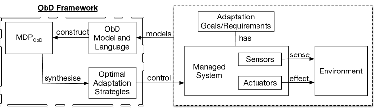
Figure 1: Framework Overview

IV ObD Modeling Language

The computation of optimal strategies is based on a domain model. A domain model specifies the environment, the capabilities of the autonomous system (or agent) and its requirements. Formally, an ObD model ($\mathcal{D}_{r}$) is a tuple $\langle\mathcal{SV},\mathcal{AD},\mathcal{ED},\mathcal{RQ},s_{c}\rangle$ where:

• $\mathcal{SV}$ is a finite set of state variables with finite domains. State variables describe the possible states, i.e., the configuration of the software system and the environment;

• $\mathcal{AD}$ is a finite set of action descriptions representing the means that are available to the agent to change the system state, i.e. update the state variables $\mathcal{SV}$;

• $\mathcal{ED}$ is a finite set of event descriptions to represent the uncontrollable occurrences in the environment, i.e., events that change the state beyond the agent’s control.

• $\mathcal{RQ}$ is a finite set of requirements, i.e., the (operationalisable) goals that the software system should satisfy;

• $s_{c}$ is the initial state of the system determined by the agent’s monitoring components and sensors.

An ObD model has a corresponding textual representation called its domain description. It is formalized in the following using a variant of Backus-Naur Form (BNF): the names enclosed in angular brackets identify non-terminals, names in bold or enclosed within quotation marks are terminals, optional items are enclosed in square brackets, $|$ is ”or”, items repeated one or more times are suffixed with $+$ and parentheses are used to group items together.

IV-A State, Actions and Events

State Variables ($\mathcal{SV}$)

define the possible states, i.e., configurations of the software system and the environment. A variable $x\in\mathcal{X}_{s}$ is a multi-valued variable with a corresponding domain, denoted $dom(x)$. Every value $y\in dom(x)$ is a configuration of $x$. A state variable is defined as follows:

$$\langle SV\rangle::=\textbf{Variable}\textbf{ }\langle ID\rangle\,\textbf{domain}\,``\{"\,\langle VALS\rangle\,``\}"$$

$$\langle VALS\rangle::=\langle ID\rangle\,|\,\langle ID\rangle\,``,"\,\langle VALS\rangle$$

where $\langle ID\rangle$ is text, i.e., a concatenation of letters, digits and symbols. For example, we can represent the location of $RoboX$ and the status of tables at the restaurant using the following variables:

$$\textbf{Variable }location\textbf{ domain }\{atTable_{1},atTable_{2},atTable_{3},$$

$$\hskip 14.22636pt\hskip 14.22636ptatTable_{4},inDining\_room,inKitchen,inOffice\}$$

$$\textbf{Variable }table_{i}\hskip 28.45274pt(\forall\,1\leq i\leq 4)$$

$$\hskip 14.22636pt\textbf{ domain }\{empty,occupied,requested,received,$$

$$\hskip 14.22636pt\hskip 14.22636ptin\_preparation,ready,collected,delivered,paid\}$$

The variable $location$ defines the possible locations of $RoboX$. The variables $table_{i}$ represent the status of tables: when there are no customers at $table_{i}$, then $table_{i}\text{=}empty$. When a customer arrives and sits at the table, $table_{i}$ becomes $occupied$. Figure 2 depicts the update of the value of $table_{i}$ with the occurrence of the robot actions {get_order, give_order, collect_order, deliver_ order, clean_table} and the exogenous events {customer_arrives, customer_orders, kitchen_notification, customer_pays}. In contrast to actions, exogenous events have an occurrence probability denoting their likelihood in a given situation. Actions, on the other hand, have a cost that represent the effort or price of their execution. Both exogenous events and actions do not have to be deterministic, i.e., their execution can have various effects, each with a different probability (in pink in the figure).

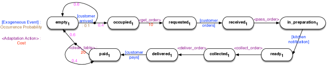
Figure 2: A simplified model of serving a table at restaurant $FoodX$.

Variables which are not explicitly defined are considered to be boolean, i.e., their domain is $\{tt,\textit{ff}\}$. The notations $id$ and $!id$ are used as shortcuts for $id\text{=}tt$ and $id\text{=}\textsl{ff}$, respectively. The following declaration defines a boolean variable to represent that customers sitting at a table had looked at the menu.

$$\textbf{Variable }looked_{i} (\forall\,1\leq i\leq 4)$$

Actions ($\mathcal{AD}$)

are means that are available to the agent to change the system state. An action description is an expression $\langle AD\rangle$ that is defined as follows:

$$\langle AD\rangle::=\textbf{Action}\,\langle ID\rangle\,\langle PEFFS\rangle^{+}\,[\textbf{cost}\,\langle\mathds{N}\rangle]$$

$$\langle PEFFS\rangle::=\textbf{ if }\langle CND\rangle\textbf{ effects }\langle EFFS\rangle^{+}$$

$$\langle EFFS\rangle::=``\langle"\langle EFF\rangle^{+}\,[\textbf{prob }\langle P\rangle]``\rangle"$$

$$\langle CND\rangle::=\langle ATOM\rangle\,|\,\langle BL\rangle\,|\,``!"\langle CND\rangle\,|\,\langle CND\rangle$$

$$\hskip 14.22636pt\,``{\bf\&}"\,\langle CND\rangle\,|\,\langle CND\rangle\,``{\bf||}"\,\langle CND\rangle\,|\,``("\langle CND\rangle``)"$$

$$\langle EFF\rangle::=\langle ID\rangle``{\bf=}"\langle ID\rangle$$

$$\langle ATOM\rangle::=\langle ID\rangle\,|\,``!"\langle ID\rangle\,|\,\langle ID\rangle``{\bf=}"\langle ID\rangle$$

$$\langle BL\rangle::=``true"\,|\,``false"$$

Actions can have a cost representing the difficulty level or effort necessary to execute it. Action costs are useful to trade-off the satisfaction of requirements with the required effort and, when not specified, are set to zero. In the following example, the cost of moving to $table_{i}$ is set to $10$.

$$\textbf{Action }move\_to\_kitchen\textbf{ if }location\text{=}inDining\_room$$

$$\hskip 14.22636pt\textbf{ effects }\langle location\text{=}inKitchen\textbf{ prob }0.8\rangle$$

$$\hskip 28.45274pt\langle location\text{=}inDining\_room\textbf{ prob }0.2\rangle\hskip 14.22636pt\textbf{ cost }10$$

Note that an expression $\langle AD\rangle$ is well-formed only if (1) its various $\langle CND\rangle$ are disjoint, i.e., they cannot be satisfied at the same time and (2) for every $\langle PEFFS\rangle$, the sum of the probabilities $\langle P\rangle$ of its subexpressions $\langle EFFS\rangle$ is one, i.e., $\sum_{i=1}^{|\langle EFFS\rangle|}\langle P\rangle=1$. Note that we allow $\sum_{i=1}^{|\langle EFFS\rangle|}\langle P\rangle$ to be less than one. In this case, action execution has no effect with a probability of $1-\sum_{i=1}^{|\langle EFFS\rangle|}\langle P\rangle$. For example, this makes it possible to remove the second effect, $\langle location=inDining\_room\textbf{ prob }0.2\rangle$, from the previous action description without affecting the action semantics.

Events ($\mathcal{EV}$)

represent occurrences that are not controlled by the agent. They may happen in the environment at any moment. An event description is expressed as follows:

$$\langle EV\rangle::=\textbf{Event}\,\langle ID\rangle\,\langle PEFFS\rangle^{+}$$

$$\langle PEFFS\rangle::=\textbf{ if }\langle CND\rangle\,[\textbf{occur prob}\,\langle P\rangle]\,\textbf{ effects }\langle EFFS\rangle^{+}$$

Events are conditional and can occur with a different probability depending on the situation. For instance, we can represent that customers may order with a higher probability if they had looked at the menu as follows:

$$\textbf{Event }request\_to\_order_{i}\hskip 28.45274pt(\forall\,1\leq i\leq 4)$$

$$\hskip 14.22636pt\textbf{ if }table_{i}\text{=}occupied\,\&\,looked_{i}\textbf{ occur prob }0.9$$

$$\hskip 28.45274pt\textbf{ effects }\langle table_{i}\text{=}requested\rangle$$

$$\hskip 14.22636pt\textbf{ if }table_{i}\text{=}occupied\,\&\,!looked_{i}\textbf{ occur prob }0.2$$

$$\hskip 28.45274pt\textbf{ effects }\langle table_{i}\text{=}requested\rangle$$

IV-B Requirements

Requirements represent the objectives of the autonomous system. Every requirement is associated with a reward denoting its importance. ObD currently supports fourteen requirement types, which build upon and extend the goal patterns of the KAOS goal taxonomy [24]. Requirements are expressions:

$$\langle RE\rangle::=\textbf{ ReqID }\langle ID\rangle\,\langle REP\rangle$$

$$\langle REP\rangle::=((\langle UA\rangle\,|\,\langle UM\rangle\,|\,\langle CA\rangle\,|\,\langle DEA\rangle\,|\,\langle DFA\rangle\,|\,\langle CM\rangle\,|$$

$$\hskip 14.22636pt\,\langle DEM\rangle\,|\,\langle DFM\rangle\,\langle PM\rangle\,|\,\langle PDEM\rangle\,|\,\langle PDFM\rangle)\,[\textbf{reward }\mathds{N}])\,|\,$$

$$\hskip 14.22636pt((\langle RPM\rangle\,|\,\langle RPDEM\rangle\,|\,\langle RPDFM\rangle)\,[\textbf{reward\_once }\mathds{N}])$$

A requirement’s type is determined based on whether it: is conditional (C) or unconditional (U); is a maintain (M) or achieve (A) requirement: duration of maintain requirements can be time-limited and its compliance can be best-effort (P) or strict (PR), i.e., during its duration the requirement does not have to be “always” satisfied; has a deadline (D), which can be exact (E), i.e., the requirement has to be satisfied at the deadline, or flexible (F), the requirement has to be satisfied within the deadline. Due to space limitations, we only present unconditional, conditional and achieve deadline requirements.

Unconditional Requirements: denote conditions that have to be always maintained or (repeatedly) achieved.

$$\langle UA\rangle::=\textbf{achieve}\,\langle CND\rangle \langle UM\rangle::=\textbf{maintain}\,\langle CND\rangle$$

For example, a $\langle UM\rangle$ requirement to remain in the dining room or an $\langle UA\rangle$ to ensure that $table_{1}$ repeatedly pays.

$$\textbf{ReqID }req_{1}\textbf{ maintain }location\text{=}inDining\_room$$

$$\textbf{ReqID }req_{2}\textbf{ achieve }table_{1}\text{=}paid$$

Conditional Requirements: should be satisfied only after some given conditions are true. They can have a cancellation condition after which their satisfaction is no longer required.

$$\langle CA\rangle::\text{=}\textbf{achieve}\,\langle CND\rangle\,\textbf{if}\,\langle CND\rangle\,[\textbf{unless}\,\langle CND\rangle]$$

$$\langle CM\rangle::\text{=}\textbf{maintain}\langle CND\rangle\textbf{if}\langle CND\rangle\,[\textbf{unless}\,\langle CND\rangle]$$

For example, $RoboX$ may have to get the order from $table_{i}$ only if $table_{i}$ requests to order, or it should remain in the dining room after it gets $table_{1}$ until $table_{1}$’s order is served.

$$\textbf{ReqID }req_{3}\textbf{ achieve }table_{i}\text{=}received$$

$$\hskip 14.22636pt\textbf{ if }table_{1}=requested\textbf{ reward }100$$

$$\textbf{ReqID }req_{4}\textbf{ maintain }location=inDining\_room$$

$$\hskip 2.84544pt\textbf{ if }table_{1}\text{=}requested\textbf{ unless }table_{1}\text{=}received\textbf{ reward }100$$

Deadline Requirements: must be satisfied after an exact number of time instants or within a period of time:

$$\langle DEA\rangle::=\textbf{achieve}\,\langle CND\rangle\,\textbf{after}\,\mathds{N}_{+}\,\textbf{if}\,\langle CND\rangle\,[\textbf{unless}\,\langle CND\rangle]$$

$$\langle DFA\rangle::=\textbf{achieve}\,\langle CND\rangle\,\textbf{within}\,\mathds{N}_{+}\,\textbf{if}\,\langle CND\rangle\,[\textbf{unless}\,\langle CND\rangle]$$

For example, $RoboX$ may have to be at $table_{1}$ within at most 4 time units after $table_{1}$ requests to place an order, or it may have to be at the kitchen after exactly 4 time units after it receives a notification that food is ready.

$$\textbf{ReqID }req_{5}\textbf{ achieve }location\text{=}atTable_{1}\textbf{ within }4$$

$$\hskip 14.22636pt\textbf{ if }table_{1}\text{=}requested\textbf{ reward }100$$

$$\textbf{ReqID }req_{6}\textbf{ achieve }location\text{=}inKitchen\textbf{ after }4$$

$$\hskip 14.22636pt\textbf{ if }table_{1}\text{=}ready\textbf{ reward }100$$

In the following, we use the terms name, required condition, activation condition, cancellation condition and deadline to refer to the parts of a requirement expression that come after $`\text{ReqID'}$, $`\text{achieve'}$ or $`\text{maintain'}$, $`\text{if'}$, $`\text{unless'}$ and $`\text{after'}$ or $`\text{within'}$ parts of the requirement expression respectively.

V Controller Synthesis

Markov Decision Processes (MDPs) are mathematical frameworks for modeling and controlling stochastic dynamical systems [17]. Informally, MDPs may be viewed as Labeled Transition Systems (LTSs) where transitions are probabilistic and can be associated to rewards. Intuitively, solving an MDP means finding an optimal strategy, i.e., determining the actions to execute in every state in order to maximize the total expected rewards. In the following, we first introduce MDPs (Section V-A), then we discuss the main steps needed to construct an MDP starting from an ObD domain model (Section V-B).

V-A Introduction to MDPs with Rewards

A reward $MDP$ is a tuple $\langle\mathcal{S},\mathcal{A},\mathcal{T},\mathcal{R},\gamma\rangle$, where:

• $\mathcal{S}$ is the finite set of all possible states of the system, also called the state space;

• $\mathcal{A}$ is a finite set of actions;

• $\mathcal{T}:\mathcal{S}\times\mathcal{A}\times D(\mathcal{S})$ where $D(\mathcal{S})$ is the set of probability distributions over states $S$. A distribution $d(S)\in D(S):S\rightarrow[0,1]$ is a function such that $\Sigma_{s\in S}d(s)=1$. The transition relation $\mathcal{T}(s_{i},a,d)$ specifies the probabilities $d(s_{j})$ of going from state $s_{i}$ after execution of action $a$ to states $s_{j}$. In the following, we will use the (matrix) notation $Pr_{a}(s_{i},s_{j})$ to represent the probability $d(s_{j})$ of going to $s_{j}$ after execution of $a$ in $s_{i}$;

• $\mathcal{R}:\mathcal{S}\times\mathcal{A}\times\mathcal{S}\rightarrow\mathds{R}$ is a reward function specifying a finite numeric reward value $\mathcal{R}(s_{i},a,s_{j})$ when the system goes from state $s_{i}$ to state $s_{j}$ as a result of executing action $a$. Thus, rewards may be viewed as incentives for executing actions. We will use $R_{a}(s_{i},s_{j})$ to represent $\mathcal{R}(s_{i},a,s_{j})$.

Formally, a (memoryless) strategy is a mapping $\pi:\mathcal{S}\rightarrow\mathcal{A}$ from states to actions. An optimal strategy, denoted $\pi^{*}$, is the one which maximizes the expected linear additive utility, formally defined as $V^{\pi}(s)=\mathds{E}[\sum_{t^{\prime}=0}^{\infty}\gamma^{t^{\prime}}R^{\pi_{s}}_{t+t^{\prime}}]$. Intuitively, this utility states that a strategy is as good as the amount of discounted reward it is expected to yield [25]. Setting $\gamma=1$ expresses indifference of the agent to the time in which a particular reward arrives; setting it to a value $0\leq\gamma<1$ reflects various degrees of preference to rewards earned sooner.

MDPs have a key property: solving an MDP finds an optimal strategy $\pi^{*}$, which is deterministic, Markovian and stationary. This means that computed strategies are independent of both past actions/states and time, which ensures their compactness and practicality. Furthermore, there exist practical algorithms for solving MDPs, e.g., value iteration and policy iteration. Both of these algorithms can be shown to perform in polynomial time for fixed $\gamma$ [26].

MDPs with memoryless strategies, depicted in Figure 5 (rounds are states and rounded squares are events), have however the following restrictions:

The implicit-event action model [17]

MDPs do not support an explicit representation of exogenous events. Figure 5 shows exogenous events (in non-rounded squares connected with pointed line to states) that can occur with certain occurrence probabilities (in green in the figure) in every state. Exogenous events are an essential element to model aspects of the environment that are not controllable by the agent. They are the means to represent, for example, that customers can arrive at the restaurant or that they may request to order.

The Markovian assumption [16, 27]

in MDP, reward and transition functions have to be Markovian, i.e., they can not refer to the history of previous states or transitions. Figure 5 shows an example of a non-Markovian reward (described on the dashed transition), i.e., one that is entailed only if certain conditions are satisfied on the history of states and transitions. The support of non-Markovian rewards is necessary to associate transitions that satisfy requirements [6], which are often conditional and can have deadlines, with rewards.

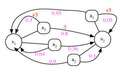
Figure 3: Basic MDP model

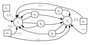
Figure 4: Support of Exogenous Events

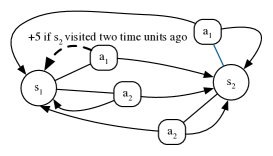
Figure 5: Support of Non-Markovian Rewards

V-B Overview of the Construction of MDPs from ObD Models

The construction of MDPs based on ObD models relies on the following intuitions:

• the states and the (probabilistic) transitions of the LTS behind the MDP are constructed based on the variables, actions and events in the ObD domain model;

• the rewards in the MDP are associated with transitions that lead to the satisfaction of requirements.

Dealing with the Markovian assumption

Building an MDP from an ObD model requires the satisfaction of the Markovian assumption. In the context of this work, determining the satisfaction of requirements, with the exception of unconditional requirements, requires to keep track of history. To solve this issue, we extend the state space to store information that is relevant to determine the status of requirements in every state. This is done by associating every requirement with a state variable, whose value reflects the status of the requirement in the state. The value of those variables, called requirements variables, are updated whenever their corresponding requirement is activated, canceled, satisfied, etc.

Requirements Variables $\mathcal{RV}$ are special variables whose domain represents all the possible statuses of their corresponding requirement. The statuses of requirements and their update after requirement activation, cancellation, satisfaction, etc are defined in the transitions part of Figures 8 and 9. On the other hand, the rewards part defines transitions that satisfy requirements and, consequently, entail a reward.

For example, consider a conditional achieve requirement $CA$ of the form $\textbf{ReqID}\,m\,\textbf{achieve}\,S\,\textbf{if}\,A\,\textbf{unless}\,Z\,\textbf{reward}\,r$. This requirement is associated with a requirement variable $m$ whose domain includes the requirement’s possible statutes $\{I,R\}$. The transitions part of Figure 9 shows the evolution of $CA$ requirements when their activation, cancellation and required conditions occur. It is to be read as follows: when the status is $I$ and the activation condition $A$ is true, then the status is updated to $R$. Analogously, if the status is $R$ and the cancellation condition $Z$ or the required condition $S$ is true, then the status is updated to $I$. The updating of a state variable as just described enables the definition of a Markovian reward when requirements are satisfied. The rewards part of Figure 9 shows transitions of $CA$ requirements that entail rewards. This figure should be read as follows: a requirement $m$ of type $CA$ induces a reward $r$ on a transition from a state $i$ to a state $j$ iff, in $i$, the required condition of $m$ does not hold and the status of $m$ is $R$; while $S$ holds in $j$.

Dealing with the absence of exogenous events

ObD models have explicit-event models whereas MDPs impose an implicit-event action model. To overcome this limitation, we exploit the technique proposed in [17] which enables computation of implicit-event action transition matrices from explicit-event models. The use of this technique assumes the following rules: 1) the action in which exogenous events are folded, always occurs before it and 2) events are commutative, i.e., their order of occurrence from an initial state produces the same final state. Under those assumptions, which are satisfied in our running example, the implicit-event transition matrix $Pr_{a}(s_{i},s_{j})$ of an action $a$ is computed in two steps: first, the transition matrix of $a$ (without exogenous events) and the transition matrix and occurrence vector of every event $e$ are computed separately; then, those elements are used to construct the implicit-event matrix of every action $a$. This process is illustrated in the following section using an example. Note that it is possible to integrate other (more complex) interleaving semantics into the framework if necessary by changing the technique used to compute the implicit-event transition matrix [17].

V-C MDP Construction Process

An ObD MDP $MDP_{r}=\langle\mathcal{S},\mathcal{A},\mathcal{T},\mathcal{R},\gamma\rangle$ is constructed from a model $\mathcal{D}_{r}=\langle\mathcal{SV},\mathcal{AV},\mathcal{ED},\mathcal{RQ},s_{0}\rangle$ as follows.

States $\mathcal{S}$: represent all possible configurations of the system and the environment. A state is a specific configuration, i.e., an assignment of every state variable in $\mathcal{SV}$ and requirement variable in $\mathcal{RV}$ a value from their domain.

For example, consider a domain model $\mathcal{D}_{r}$ comprising of two boolean variables $x$ and $y$ and one requirement $m$ of type $CA$. The set of states $\mathcal{S}$ constructed from $\mathcal{D}_{r}$ comprises all possible configurations of its state and requirement variables. Thus, $\mathcal{S}$ includes the eight states in Figure 6.

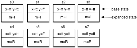
Figure 6: Constructed States

Actions $\mathcal{A}$: are all the actions appearing in $\mathcal{AV}$ of the domain model $\mathcal{D}_{r}$ extended with the empty action $noop$, which produces no effects and has no cost, i.e., $\mathcal{A}=\mathcal{AV}\cup\{noop\}$.

The transition matrix $\mathcal{T}$: is computed in two steps: first, the transition matrix of $a$ (without exogenous events) and the transition matrix and occurrence vector of every event $e$ are computed separately; then, those elements are used to construct the implicit-event matrix of every action $a$.

For example, consider that our domain model $\mathcal{D}_{r}$ includes one probabilistic action $a$, one deterministic action $b$ and one requirement $m$, which are defined as follows:

$$\textbf{Action }a\textbf{ if }!x\textbf{ effects }\langle x\textbf{ prob }0.8\rangle\langle y\textbf{ prob }0.2\rangle\;\textbf{ cost }10$$

$$\textbf{Action }b\textbf{ if }x\textbf{ effects }\langle!x\rangle\;\textbf{ cost }5$$

$$\textbf{ReqID }m\textbf{ achieve }x\textbf{ if }!x\textbf{ reward }100$$

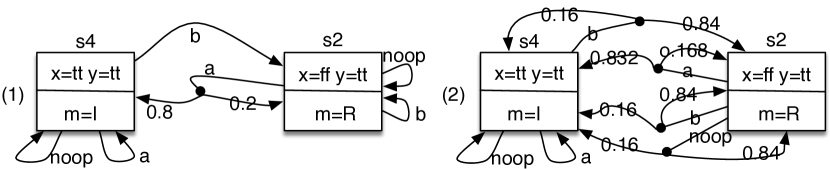
Figure 7: (1) action transitions, (2) implicit-event action transitions.

Figure 7(1) shows the transitions caused by the execution of actions in the states $s_{2}$ and $s_{4}$. For example, since the condition $!x$ is satisfied in $s_{2}$, the execution of $a$ in $s_{2}$ produces $x$ with a probability of $0.8$ and produces $y$ with a probability of $0.2$. Notice that after the execution of $a$, the base state of both $s_{0}$ and $s_{4}$ could be the result of executing action $a$ in $s_{2}$. However, since the execution of $a$ satisfies the requirement $m$, i.e., makes $x$ true, only the expanded state of $s_{4}$ satisfies the state transition model of the $CA$ requirement $m$ shown in Figure 9 since $m=I$. Thus, the execution of $a$ in state $s_{2}$ leads to $s_{0}$ with a probability $0.8$, i.e., $Pr_{a}(s_{2},s_{4})=0.8$. The execution of $b$ and $noop$ do not change the state.

Events are similar to actions with the exception that they have occurrence probabilities, do not have a cost and do not advance time since they occur concurrently with actions. Let $e$ be an event defined similarly to $a$ as follows:

$$\textbf{Event }e\textbf{ if }!x\textbf{ occur prob }0.2\textbf{ effects }\langle x\textbf{ prob }0.8\rangle\langle y\textbf{ prob }0.2\rangle$$

In this case, the transition matrix of $e$ is similar to that of $a$, i.e., $Pr_{e}=Pr_{a}$. The occurrence vector $O_{e}$ of $e$ represents the probability of occurrence of $e$ in every state. Since the condition $\neg x$ is satisfied in the states $s_{2}$, $s_{3}$, $s_{6}$ and $s_{7}$, $O_{e}(s_{2})=O_{e}(s_{3})=O_{e}(s_{6})=O_{e}(s_{7})=0.2$. Figure 7(2) shows the implicit-event transitions for the states $s_{2}$ and $s_{4}$: in $s_{2}$, event $e$ may occur with a probability of $0.2$, thus its effects are factored in action transitions as shown in Figure 7(2); in $s_{4}$, the condition of $e$ is not satisfied and, therefore, it does not affect the computed transitions for the actions $noop$ and $a$. Due to the interleaving semantics where exogenous events (may) occur after action execution, the transition caused by $b$ in $s_{4}$ is affected due to the possibility that $e$ occurs after $b$.

Construction of the reward matrix $\mathcal{R}$:

Transition rewards are affected by: (1) action costs and (2) satisfaction of requirements. In particular, a transition reward $R_{a}(s_{i},s_{j})$ is the sum of rewards obtained due to satisfaction of requirements on the transition from $s_{i}$ to $s_{j}$ minus the cost of $a$. For example, consider the transition from $s_{2}$ to $s_{4}$ caused by the execution of $a$ in $s_{2}$. On this transition, the requirement $m$ is satisfied. Since the cost of executing $a$ is $10$, this transition will be associated with a reward of $100-10=90$, i.e., $R_{a}(s_{2},s_{4})=90$.

V-D Requirements Transitions and Rewards

This section explains the key intuitions behind the modeling of requirements in ObD and their semantics.

Unconditional Achieve and Maintain Rewards

A maintain requirement defines a condition that should be kept satisfied. Therefore, a reward is given to the agent whenever this condition holds over two consecutive states, see, e.g., $\langle UM\rangle$ in Figure 8. On the other hand, an achieve requirement defines a condition that should be reached. Therefore, the agent is rewarded when this condition becomes true, i.e., when it does not hold in a state but holds in the next, e.g., see $\langle UA\rangle$.

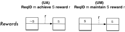
Figure 8: Unconditional Requirements States and Rewards

Conditional Requirements

The satisfaction of requirements is often necessary only after some condition $A$ becomes true, see for instance $\langle CA\rangle$ and $\langle CM\rangle$ in Figure 9. Those requirements are therefore modeled as state machines which are initially in an initial or inactive state $I$. When their activation condition $A$ occurs, a transition to a new state $R$ occurs. In a state $R$, the requirement is said to be in force, i.e., its satisfaction is required. While in $R$, the reward $r$ is obtained whenever the agent manages to comply with the required condition $S$. If the cancellation conditions $Z$ is detected while the requirement is in force, a transition to $I$ occurs, i.e., the requirement is canceled and has no longer to be fulfilled.

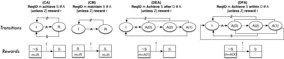
Figure 9: Conditional and Achieve Deadline Requirements States and Rewards

Deadline Achieve Requirements

Requirements are sometimes associated with fixed deadlines. Fixed deadlines can represent either an exact time after which the agent should comply with the requirement, see for example $\langle DEA\rangle$ in Figure 9; or a period of (discrete) time during which the agent may comply at any moment, see for example $\langle DFA\rangle$. In both cases, deadlines are modeled similarly. For example, consider a requirement $m$ having a deadline $D$. After $m$’s activation, a transition to a state $A(D)$ occurs. At every subsequent time unit, a transition from a state $A(X)$ to a state $A(X-1)$ occurs (unless $X=1$). A transition entails the requirement’s reward if the requirement is satisfied on this transition.

VI Evaluation

In this section, we first present an empirical evaluation of the framework by comparing the use of an ObD controller to control $RoboX$ in a simulated software environment of the restaurant $FoodX$ to a generic Monitor Analyze Plan Execute (MAPE) controller (Section VI-A). The MAPE controller relies on a Planning Domain Description Language (PDDL) planner, similarly to state-of-the-art robotic systems such as ROS [28]. Then, we present a qualitative comparison of ObD with state-of-the-art probabilistic model-checkers, PAT [29], PRISM [15] and STORM [30] which have been used in several other previous works [12, 13, 5, 14] to solve adaptation problems (Section VI-B). Finally, we describe the current prototype tool implementation and conduct a performance evaluation (Section VI-C).

VI-A Empirical Evaluation

Figure 12 depicts our simulation environment. It consists of a system state, an agent and an environment. The simulation runs in discrete time steps. At each step, the agent has to choose, based on the current system state, one action to execute from actions whose preconditions are satisfied in the state. On the other hand, some events are selected for execution, according to their occurrence probability, if their preconditions are true. After each time step, the state is updated by applying the effects of the chosen action and events in the current state. Effects of both actions and events are applied probabilistically according to the probabilities specified in their action/event descriptions, i.e. their execution can lead to different states. Experiments are run for one hundred thousands steps.

To select the agent’s actions, two controllers were implemented: an ObD controller and a generic MAPE controller. The design rational of the experiment aims at comparing a ObD controller and generic MAPE controllers with respect to: types of supported requirements, enforcement model, response time, quality of decision-making and problem representation.

Experiment Description

The experiment ran on a MacBook pro with a 2.2GHz Intel Core i7 and 16 GB of DDR3 RAM. At each time step, the agent queries the state (the (M)onitoring activity). The agent determines its action to execute by interacting with its controller. The controller, given the current state, determines the next action of the agent. The ObD controller is implemented in Java and uses the computed ObD strategies to determine the optimal action that the agent should take at each state. The MAPE controller is also implemented in Java. It consists of three components: 1) an analysis component that determines whether planning is needed, 2) PDDL4J, an open source Java library for Automated Planning based on PDDL [31], to compute plans and 3) a plan enforcer which returns one action at each step to the agent. Below is a comparison of the two controllers.

Supported requirements

ObD supports the types of requirements presented in Section IV-B. The MAPE controller, since it relies on a PDDL planer, can naturally encode unconditional and conditional achieve requirements, i.e. $\langle UA,CA\rangle$. The other types of requirements cannot be easily encoded in the form of PDDL planning problems.

Enforcement model

The ObD controller enforces MDP strategies. It has a simple enforcement model: it consults the computed strategy and determines the optimal action that corresponds to the current state at each time step. The MAPE controller enforces requirements as follows: if the activation condition of a conditional requirement is true in the state then a planning problem (Pb) is formulated to satisfy the requirement’s condition. When multiple requirements must be satisfied, then the goal state of the planning problem corresponds to the disjunction of their (satisfaction) conditions, i.e. one requirement should be satisfied. If a plan (P) is found by the PDDL planner, the plan enforcer module selects one action of P to return to the agent at each time step. A plan is pursued until its end, i.e. no re-planning is performed until the plan’s last action is executed unless a plan execution fails. A plan fails if one of its actions cannot be executed because its preconditions are not satisfied in the current state. This situation may occur due to nondeterministic action effects or event occurrences.

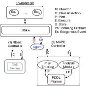
Figure 10: Experiment Description

Figure 11: Decision-making time per time step

Figure 12: Goal satisfaction per time step

Response time

Figure 12 shows the average time of decision making, i.e. the total decision-making time divided by the total number of steps of the experiment. Several domain descriptions differing in their total number of planning goals/requirements and action success rate (100%-50%) are considered. The decision time of an ObD controller is constant and almost instantaneous ($\sim$200ns) as it consists of a simple lookup in the policy (which is stored in the form of an array of Integers) of the optimal action that corresponds to the current state. On the other hand, the analysis and planning activities of the MAPE controller introduce a significant overhead when compared to the ObD controller. The average decision-making time of MAPE controllers also increases with action non-determinism as re-planning is required more frequently due to more frequent plan failures.

Quality of decision-making

Figure 12 shows the number of satisfied goals per time step for MAPE and ObD controllers. It demonstrates that the ObD controllers consistently outperform MAPE controllers for the same domain problems. This is due, on one hand, to their ability to include probabilities of event occurrences into their computation of optimal strategies. For instance, imagine that $RoboX$ has to pass the order of a table to the kitchen but that it estimates that there is a high-likelihood that another table orders. In this case, the ObD controller may delay moving to the kitchen to pass the order and wait until the other table orders first before passing the two orders to the kitchen together. MAPE controllers are incapable of incorporating such intelligence in their decision-making. Another reason explaining this result is that MAPE controllers, once a plan is computed, commit to it unless the plan fails to avoid getting stuck in re-planning without acting, which could happen if the frequency of change in the environment is high. This makes it impossible to guarantee the optimality of plans throughout their execution. On the other hand, ObD strategies are guaranteed to always select the optimal action at each state.

Representation

An important difference is the goal/requirement representation. In MAPE, planning goals have to be satisfiable using solely the actions that are available to the agent. For example, consider a goal to achieve that a table pays as many times as possible. The satisfaction of this goal requires interactions with the environment as described in Figure 2. This requirement cannot therefore be expressed as a single planning goal but has to be decomposed into a set of planning goals, each of which has to be satisfiable by the actions available to the agent. On the other hand, thanks to the folding of events into actions, such requirements can be expressed directly in ObD. Consequently, expression of requirements in ObD can be much more succinct and enable system designers to focus of what should be satisfied rather than how they should be satisfied. In the running example, it was possible to represent four MAPE planning goals in the form of a single ObD requirement.

VI-B Qualitative Comparison of ObD with State-of-the-Art Probabilistic Model-checkers

State-of-the-art probabilistic model-checkers PAT [29], PRISM [15] and STORM [30] support the description of various models using a variety of languages. In this work, we focus on MDP models because they support, as opposed to other models such as for example Discrete-Time Markov Chains, the synthesis of optimal strategies. With respect to the general-purpose languages proposed by probabilistic model-checkers, our model and language support exogenous events and various typical software requirements (Section IV-B), elements that cannot be modeled or expressed using the general-purpose MDP languages of PAT, PRISM or Storm. An extension of PRISM, namely PRISM-games, supports modeling of turn-based multi-player stochastic games. This enables the modeling of the environment as a separate player whose actions represent exogenous events. With respect to modeling of autonomous systems and their requirements, PRISM-games has two main limitations. First, similarly to PRISM, rewards have to be Markovain which means that there is no way to encode typical software requirements [6] such as those presented in Section IV-B using the provided (Markovian) reward structures. Furthermore, modeling of interactions between the agent and its environment in ObD where multiple events occur with each action of the decision maker is more realistic and natural than, in turn-based PRISM-games, where the environment may only be represented in the form of a separate player who selects at most one event to execute after each action of the decision maker.

VI-C Preliminary Experimental Evaluation

We have implemented the ObD framework as a Java-based prototype which uses EMFText [32], the MDPToolBox package [33] and Graphviz [34]. There are at least two main use cases of the framework:

At design-time

the textual editor generated by EMFText can be used to define ObD models. The corresponding MDP models and optimal strategies can be then visualized and inspected by a system designer and/or used to synthesize optimal controllers for the target autonomous systems;

At runtime

the ObD Java API can be used to create instances of the ObD model and the computation of optimal strategies at runtime. At runtime, strategies should be recomputed after change in either 1) requirements or 2) domain descriptions. The former generally denotes a change in system objectives or their priorities. On the other hand, the latter is needed if new information (possibly based on interactions with the environment) shows that model parameters need to be revised. There are some limitations to this use scenario which are discussed in Section VII.

Figures 14 and 14 show the MDP construction and solving time for different state space sizes, respectively. It is clear from the figures that the current implementation suffers from the state explosion problem. However, the support of thousands of states is typically sufficient for a large number of problems. Furthermore, solving an MDP is a one-time effort, i.e. once an MDP is solved (given a set of requirements), the computed strategies can be used until either requirements or the domain model change.The improvement of the performance of our current prototype represents future work.

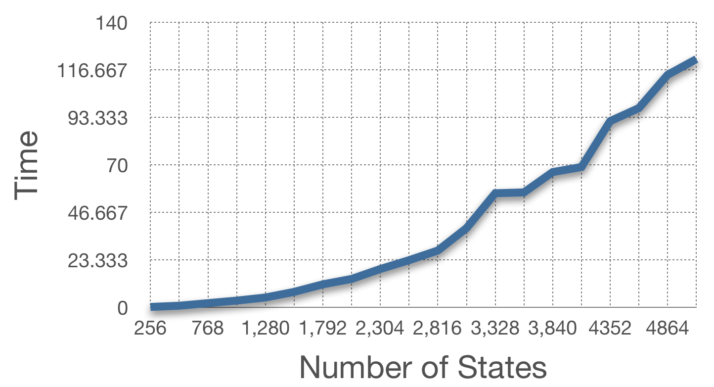
Figure 13: MDP Construction

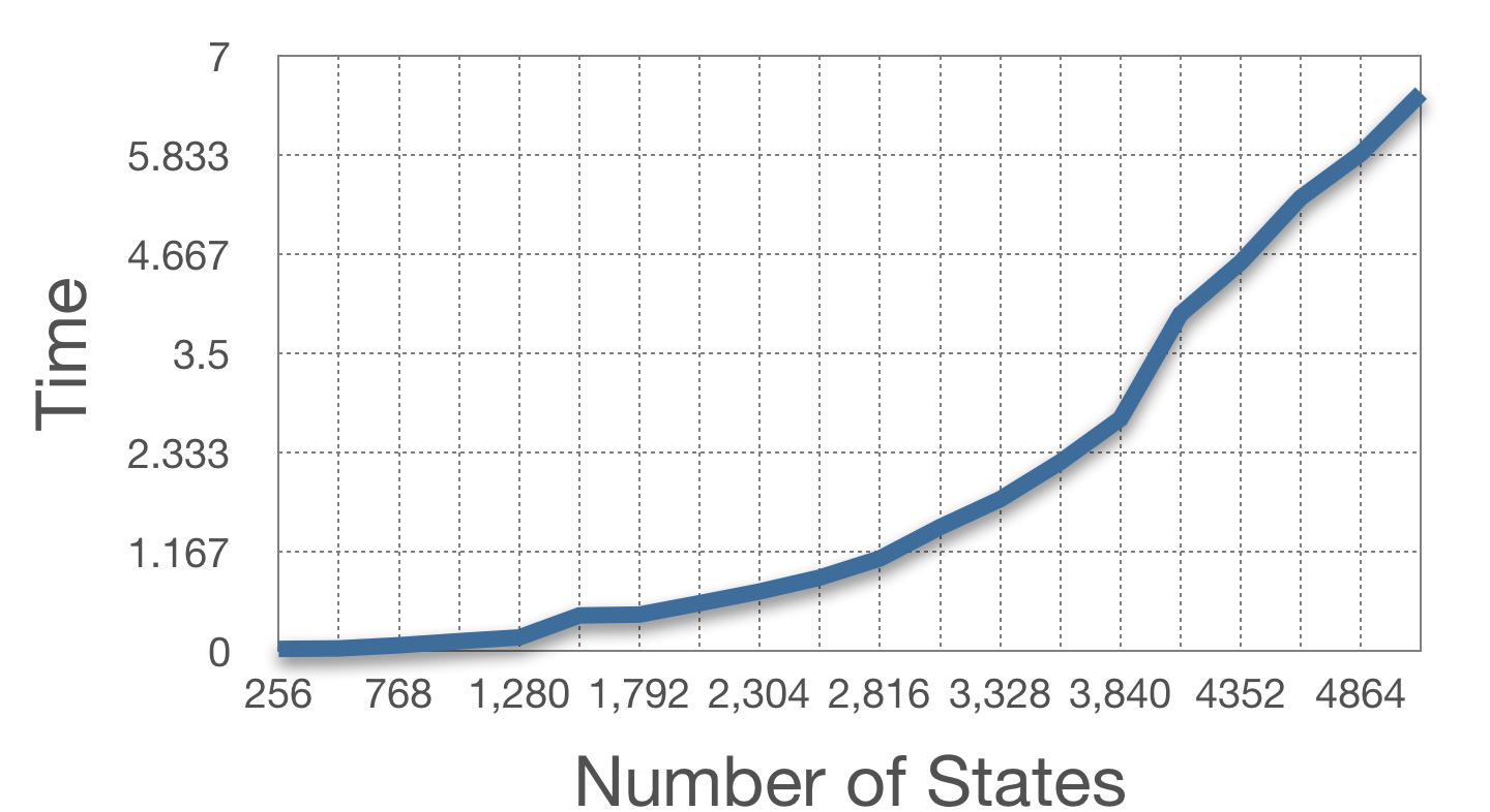
Figure 14: MDP Solution

VII Limitations & Issues

This section discusses the current limitations and issues related to using ObD and means to address them.

Setting of Model parameters

determining probabilities of actions and events can be challenging. We envisage that they shall be computed by adapting existing techniques that enable computation and learning of model parameters at runtime. For example, we could use [35] where Bayesian techniques are used to re-estimate probabilities in formal models such as Markov chains based on real data observed at runtime; or [36] which proposes an on-line learning method that infers and dynamically adjusts probabilities of Markov models from observations of system behaviour. Alternatively, reinforcement learning techniques [37] could be used.

Identification of requirements

strategies are computed according to requirements. It is thus crucial that they be correctly identified. ObD supports traditional goal modeling techniques [38, 39, 40]. Those techniques have been proven reliable over the years in ensuring correct elicitation, refinement, analysis and verification of requirements [38, 39, 40].

Suitability of the Application Domain

it is necessary to identify system conditions under which the framework may be used. Towards answering this question, we first define a predictable (unpredictable) system as one where probabilities of occurrence and effects of events/actions do not (do) change with time. Similarly, we define a dynamic (erratic) system as one where the rate of relevant change in those probabilities is within the order of hours or days (minutes or seconds). Our current prototype implementation computes strategies within minutes. Consequently, we conjecture that it supports the runtime synthesis of controllers in predicable and unpredictable dynamic systems. Erratic systems are not supported. A more precise definition of those limitations represents future work.

VIII Related Work

TABLE I: Comparison of ObD with Related Frameworks

Comp.	Sub-criteria	$F_{1}$	$Q_{1}$	$K_{1}$	$R_{1}$	$K_{2}$	$A_{1}$	$R$
Model	Requirements	$\checkmark$	$\checkmark$	$\checkmark$	$\checkmark$	$\checkmark$	$\checkmark$	$\checkmark$
	Capabilities	$\checkmark$	$\circ$	$\checkmark$	$\circ$	$\circ$	$\circ$	$\checkmark$
	Events	$\times$	$\circ$	$\times$	$\times$	$\circ$	$\times$	$\checkmark$
Uncert.	Occurrence	$\times$	$\circ$	$\times$	$\times$	$\circ$	$\times$	$\checkmark$
	Effects	$\times$	$\circ$	$\times$	$\checkmark$	$\circ$	$\times$	$\checkmark$
Adapt	Explicit	$\checkmark$	$-$	$\checkmark$	$\checkmark$	$-$	$\checkmark$	$-$
	Configuration	$-$	$\checkmark$	$-$	$-$	$\checkmark$	$-$	$-$
	Behavior	$-$	$-$	$-$	$-$	$-$	$-$	$\checkmark$
$\checkmark$: supported                               $\times$: not supported
$\circ$: partially supported (implicit)           $-$: not applicable
$F_{1}$: FLAGS [41]     $Q_{1}$: QoSMOS [8]     $K_{1}$: KAOS [39, 24, 42]
$R_{1}$: Rainbow [43, 44]                    $K_{2}$: KAMI [45]
$A_{1}$: ActivFORMS [46]                    $R$: ObD

Table I compares the features of ObD with some notable requirements-driven adaptation frameworks according to the criteria in Sec. II, divided along the following dimensions.

Modeling compares the frameworks with respect to their support of the explicit modeling and representation of requirements, capabilities and events. Those feature are desirable as they simplify system design, its maintenance and modularity.

Uncertainty compares the support of uncertainty in exogenous event occurrences and effects.

Adaptation compares the type of adaptation strategies, which can be explicitly defined, configuration selection or behavior optimization. Configuration selection is a reactive approach where, after requirements are violated, the alternative system configurations are compared and the best one is selected. Behavior optimization is a proactive approach which takes into account not only the current conditions, but how they are estimated to evolve [12]. Only behavior-based optimization supports the two requirements of (1) proactive and long-term behavior optimization, and (2) fast and optimal response to change. Note that adaptation based on explicitly defined strategies is fast but provides no optimality guarantees.

Table I shows that adaptations in many current frameworks are either explicitly defined [24, 43, 6, 41, 44, 46, 42] or determined based on a comparison of possible system configurations [8, 45], without taking into account future evolutions of the system. It also shows that explicit-event and action models are rarely considered. For example, QosMOS and KAMI consider Markov chains. This is why these frameworks have an implicit models of actions and events in Table I. Similarly, ActivForms rely on Timed Automata and the Execute activity is explicitly defined. Therefore, ActiveForms has explicit adaptation strategies and uncertainty is not handled. In [5], MDP is used to identify optimal adaptations at runtime, taking into account the delay or latency required to bring about the effects of adaptation tactics . In [12, 14], latency-aware adaptation is studied using stochastic multi-player games (SMGs). In [13], SMGs are used to generate optimal adaptation plans for architecture-based self-adaptation. These works exploit PRISM and PRISM-games to solve adaptation problems. So, they have the limitations discussed in Section VI-B.

Several other works [47, 48, 49] studied the optimization of system configurations. In contrast, this paper focuses on behavior optimization. Several recent proposals explored the application of concepts from control theory [50, 51, 52, 53] to perform system adaptation. One main difference with respect to these works is that their focus is on the optimization of quantifiable and measurable non-functional goals, such as response time, as opposed to behavior optimization based on functional requirements, the primary focus here.

IX Conclusion

This paper introduces the ObD framework for the model-based-requirements-driven synthesis of reflex controllers for autonomous systems. The framework introduces a model and a language to describe autonomous systems, their environment and requirements. The semantics of the model is defined in the form of an MDP, which can be solved producing optimal adaptation strategies (reflex controllers) for autonomous systems. In comparison with the general-purpose languages proposed by probabilistic model-checkers, ObD solves two main limitations, namely the Markovian assumption and the implicit-event model. This enables the support of a comprehensive set of software requirements and permits the accurate modeling of the environment in which autonomous systems operate.

Future work consists of extending the framework to support online learning (reinforcement learning) [37]. The study of formal adaptation guarantees and assurances [54, 55, 56, 9], and optimizing the performance of our framework [57, 58] are other future planned extensions.

This appendix presents formally the mapping of ObD model descriptions into an MDP.

A model description is a tuple $\mathcal{D}_{r}=\langle\mathcal{SV},\mathcal{AV},\mathcal{ED},\mathcal{RQ},s_{0}\rangle$, an $MDP_{r}=\langle\mathcal{S},\mathcal{A},\mathcal{T},\mathcal{R},\gamma\rangle$ is the MDP built on the basis of $\mathcal{D}_{r}$ if its various elements are constructed as described below.

State Atoms

Let $\mathcal{SV}=\{x_{1},...,x_{n}\}$ be the set of state variables of $\mathcal{D}_{r}$ and $\{dom(x_{1}),...,dom(x_{n})\}$ be their corresponding domains. An assignment of a value $v_{i}\in dom(x_{i})$ to a state variable $x_{i}$ is called a state atom over $x_{i}$. The set of state atoms $\mathcal{SA}=\{x_{i}$=$v_{j}\,|\,x_{i}\in\mathcal{SV}\textsl{ and }v_{i}\in dom(x_{i})\}$ is called the set of state atoms of $\mathcal{D}_{r}$.

Requirement Variables and Requirement Atoms

Let $\mathcal{RQ}$ be the requirements of $\mathcal{D}_{r}$. Let $r\in\mathcal{RQ}$ be a requirement and $name(r)$, $type(r)$ and $states(r)$ be functions returning the requirement’s identifier, type and its possible states respectively. For example, let $r=\textbf{ReqID }m\textbf{ achieve }S\textbf{ if }A$ $\textbf{ unless }Z\textbf{ reward }r$. In this case, $name(r)=m$, $type(r)=CA$ and $states(r)=\{I,R\}$. The set of requirements variables of $\mathcal{D}_{r}$ is the set $\mathcal{RV}=\{r_{1},...,r_{m}\}$ such that every $r_{i}$ is the name of a different requirement in $\mathcal{RQ}$. The domain of every $r_{i}$ is its set of possible states, i.e., $dom(r_{i})=states(r_{i})$. The set $\mathcal{RA}=\{m=s\,|\,m\in\mathcal{RV}\textsl{ and }s\in dom(m)\}$ is called the set of requirement atoms of $\mathcal{D}_{r}$.

Definition 1 (States $\mathcal{S}$)

Let $\mathcal{V}$ be the set $\mathcal{SV}\cup\mathcal{RV}$. In this case, the set of states generated from $\mathcal{V}$ is the set $\mathcal{S}=\{\bigcup_{i=1}^{|\mathcal{V}|}\{x_{i}=v_{i}\}\,|\,x_{i}\in\mathcal{V}\,and\,v_{i}\in dom(x_{i})\}$.

Intuitively, the previous definition means that every state $s\in\mathcal{S}$ is a set of atoms such that a value is assigned to every variable $x\in\mathcal{V}$. A state $s$ includes both state and requirements atoms. We distinguish between them as follows: state atoms of a state $s$ are referred to as the base state of $s$, denoted $\overline{s}$, and requirement atoms are referred to as the expanded state of $s$, denoted $\dot{s}$. More formally, let $s$ be a state, $\overline{s}=\{at\,|\,at\in s,\,at\in\mathcal{SA}\}$, whereas $\dot{s}=\{at\,|\,at\in s,\,at\in\mathcal{RA}\}$. This distinction is needed as state and requirements are updated differently: state atoms are directly updated by occurrence of actions and events; on the other hand, requirements atoms are indirectly updated if their status need be updated as a result of change in state atoms.

Action Representation

Let an action expression $ad\in\mathcal{AV}$ be a tuple $ad=\langle a,cost,\langle pre_{1},\langle EF^{1}_{1},p^{1}_{1}\rangle,$ $...,\langle EF^{1}_{m},$ $p^{1}_{m}\rangle\rangle,...,\langle pre_{n},$ $\langle EF^{n}_{1},$ $p^{n}_{1}\rangle,...,\langle EF^{n}_{l},p^{n}_{l}\rangle\rangle\rangle$ where $a$ is the action name, $cost$ its cost, $pre_{i}$ is one of its preconditions, every $\langle EF^{i}_{x},p^{i}_{x}\rangle$ is one effect $x$ of the execution of $a$ when the precondition $pre_{i}$ holds and $p^{i}_{x}$ is the probability of producing the effect $x$.

Definition 2 (Actions)

The set of actions $\mathcal{A}$ is the set of action names in $\mathcal{AV}$ and the noop action, i.e., $\mathcal{A}$ is $\{a\,|\,\langle a,cost,\langle pre_{1},\langle EF^{1}_{1},p^{1}_{1}\rangle,$ $...,\langle EF^{1}_{m},$ $p^{1}_{m}\rangle\rangle,...,\langle pre_{n},$ $\langle EF^{n}_{1},$ $p^{n}_{1}\rangle,...,\langle EF^{n}_{l},p^{n}_{l}\rangle\rangle\rangle\in\mathcal{AV}\}\cup\{noop\}$ where $noop$ is an action which execution has no cost and produces no effects.

Formula Satisfaction

Let $f$ be a formula of the form $6$ and $Y$ a set of atoms. The satisfaction of a formula $f$ in $Y$, denoted $Y\models f$, is defined in the usual way as follows:

$$Y\models at \textbf{ iff }at\in Y\textbf{ otherwise }Y\not\models at$$

$$Y\models!f \textbf{ iff }Y\not\models f$$

$$Y\models f_{1}\,\&\,f_{2} \textbf{ iff }Y\models f_{1}\text{ and }Y\models f_{2}$$

$$Y\models f_{1}\,||\,f_{2} \textbf{ iff }Y\models f_{1}\text{ or }Y\models f_{2}$$

Action Execution

Let $s$ be a state and $ad=\langle a,cost,\langle pre_{1},\langle EF^{1}_{1},p^{1}_{1}\rangle,$ $...,\langle EF^{1}_{m},p^{1}_{m}\rangle\rangle,...,\langle pre_{n},$ $\langle EF^{n}_{1},$ $p^{n}_{1}\rangle,...,\langle EF^{n}_{l},p^{n}_{l}\rangle\rangle\rangle\in\mathcal{AV}$ be the action description of $a\in\mathcal{A}$ in $\mathcal{D}_{r}$. The execution of $a$ in $s$ produces a state $r$ with a probability $p$ iff:

• a precondition $pre_{i}$ of the action description $ad$ is satisfied in $s$, i.e., $s\models pre_{i}$,

• one of the effects in $EF^{i}_{j}$ of $pre_{i}$ is $eff=\{l_{1},...,l_{n}\}$,

• the probability $p$ is $p^{i}_{j}$,

• the state $r$ satisfies the following two conditions:

  • its base state is $\overline{s}$ after the update of the value of every state variable in which appears in $EF^{i}_{j}$ with the value specified in $EF^{i}_{j}$. Formally, this is represented as follows: $\overline{r}=(\overline{s}\setminus chg(\overline{s},EF^{i}_{j}))\cup EF^{i}_{j}$ where $chg(\overline{s},EF^{i}_{j})=\{x=v\,|\,x=v^{\prime}\in EF^{i}_{j},x=v\in\overline{s}\}$,

  • its expanded state is $\dot{s}$ after the update of the state of every requirement according the state transition models shown in Fig. (8)(9)(15). Formally, $\dot{r}=\{upd_{T}(m,st,\overline{r})\,|\,m=st\in\dot{s}\text{ and }type(m)=T\}$ where $upd_{T}(m,st,x)$ defines how the requirement $m$ of type $T$ should be updated when its current state is $st$ and the newly computed base state is $x$. This function is defined for every type of requirements according to its state transition model. For example, consider $PM$ requirements of the form $\textbf{ReqId }m\textbf{ maintain }S\textbf{ for }P$ $\textbf{ if }A\textbf{ unless }Z$ $\textbf{reward }r$, the definition of $upd_{PM}(m,st,x)$ is as follows:

    $\displaystyle upd_{PM}(m,st,x)=\left.\begin{cases}m=A,&\text{if }st=I\text{ and }x\models A\\ m=I,&\text{if }st=A\text{ and }x\models Z\\ m=R(P),&\text{if }st=A\text{ and }x\models(S\,\&\,!Z)\\ m=I,&\text{if }st=R(T)\text{ and }x\models Z\\ m=I,&\text{if }st=R(1)\\ m=R(T-1),&\text{if }st=R(T)\text{ and }x\not\models Z\text{ and }T\neq 1\\ m=st,&\text{otherwise }\end{cases}\right.$

• Otherwise, if none of the action preconditions is true in $s$, then $\overline{r}=\overline{s}$, $\dot{r}=\{upd_{T}(m,st,\overline{r})\,|\,(m=st)\in\dot{s}\text{ and }type(m)=T\}$ and $p=1$.

Other functions are similarly defined to describe the update of the state of the other types of requirements as shown in the transitions part of Fig. (8)(9)(15). We define similarly the execution of an event $e$ in a state $s$ as follows.

Event Execution

Let $s$ be a state and $\langle e,\langle pre_{1},op_{1},\langle EF^{1}_{1},p^{1}_{1}\rangle,...,$ $\langle EF^{1}_{m},p^{1}_{m}\rangle\rangle,...,\langle pre_{n},op_{n},$ $\langle EF^{n}_{1},$ $p^{n}_{1}\rangle,...,\langle EF^{n}_{l},p^{n}_{l}\rangle\rangle\rangle\in\mathcal{ED}$ be the event description $ev$ of an event $e$ in $\mathcal{D}_{r}$. The execution of $e$ in $s$ produces a state $r$ with a probability $p$ iff:

• a precondition $pre_{i}$ is satisfied in $s$, i.e., $s\models pre_{i}$,

• one of the effects in $EF^{i}_{j}$ of $pre_{i}$ is $eff=\{l_{1},...,l_{n}\}$,

• the probability $p$ is $p^{i}_{j}$,

• the state $r$ satisfies the following two conditions:

  • its base state is $\overline{s}$ after the update of the value of every state variable in which appears in $EF^{i}_{j}$ with the value specified in $EF^{i}_{j}$. Formally, this is represented as follows: $\overline{r}=(\overline{s}\setminus chg(\overline{s},EF^{i}_{j}))\cup EF^{i}_{j}$ where $chg(\overline{s},EF^{i}_{j})=\{x=v\,|\,x=v^{\prime}\in EF^{i}_{j},x=v\in\overline{s}\}$,

  • its expanded state is $\dot{s}$ after the update of the state of every requirement according the state transition models shown in Fig. (8)(9)(15). Formally, $\dot{r}=\{upd^{e}_{T}(m,st,\overline{r})\,|\,m=st\in\dot{s}\text{ and }type(m)=T\}$ where $upd^{e}_{T}(m,st,x)$ defines how the requirement $m$ of type $T$ should be updated when its current state is $st$ and the newly computed base state is $x$ due to an event occurrence. The function $upd^{e}_{T}(m,st,x)$ is defined similarly to $upd_{T}(m,st,x)$ with the exception that events do not cause time-related transitions in the requirements’ state machines since they occur concurrently with actions. For example, consider $PM$ requirements of the form $\textbf{ReqId }m\textbf{ maintain }S\textbf{ for }P\textbf{ if }$ $A\textbf{ unless }Z\textbf{ reward }r$, the definition of $upd^{e}_{PM}(m,st,x)$ is as follows:

    $\displaystyle upd^{e}_{PM}(m,st,X)=\left.\begin{cases}m=A,&\text{if }st=I\text{ and }x\models A\\ m=I,&\text{if }st=A\text{ and }x\models Z\\ m=R(P),&\text{if }st=A\text{ and }x\models(S\,\&\,!Z)\\ m=I,&\text{if }st=R(T)\text{ and }x\models Z\\ m=I,&\text{if }st=R(1)\\ m=st,&\text{otherwise }\end{cases}\right.$

• Otherwise, if none of the event preconditions is true in $s$, then $\overline{r}=\overline{s}$, $\dot{r}=\{upd^{e}_{T}(m,st,\overline{r})\,|\,(m=st)\in\dot{s}\text{ and }type(m)=T\}$ and $p=1$.

Event Occurrence Vector

Let $s$ be a state and $\langle e,\langle pre_{1},op_{1},\langle EF^{1}_{1},p^{1}_{1}\rangle,$ $...,\langle EF^{1}_{m},p^{1}_{m}\rangle\rangle,$ $...,$ $\langle pre_{n},op_{n},$ $\langle EF^{n}_{1},$ $p^{n}_{1}\rangle,...,\langle EF^{n}_{l},p^{n}_{l}\rangle\rangle\rangle\in\mathcal{ED}$ be an event description $ed$ of an event $e$ in $\mathcal{D}_{r}$. The occurrence vector of $e$ is a vector $O_{e}$ of length $|\mathcal{S}|$ whose entries are defined as follows:

$\displaystyle O_{e}(s)=\left.\begin{cases}op_{i}&\text{if }s\models pre_{i}\\ 0&\text{otherwise }\end{cases}\right.$

Explicit Action Transition Matrix

Let $a\in\mathcal{A}$ be an action and $\mathcal{S}$ be the set states. The explicit transition matrix of $a$, denoted $Pr_{a}$, is a $|\mathcal{S}|\times|\mathcal{S}|$ matrix. If the execution of $a$ in a state $s\in\mathcal{S}$ produces the state $r\in\mathcal{S}$ with a probability $p$, then $Pr_{a}(s,r)=p$.

Explicit Event Transition Matrix

Let $e$ be an event and $\mathcal{S}$ be the set states. The explicit transition matrix of $e$, denoted $Pr_{e}$, is a $|\mathcal{S}|\times|\mathcal{S}|$ matrix. If the execution of $e$ in a state $s\in\mathcal{S}$ produces the state $r\in\mathcal{S}$ with a probability $p$, then $Pr_{e}(s,r)=p$.

Effective Events Transition Matrix

Let $Pr_{e_{1}},...,Pr_{e_{n}}$ be the explicit event transition matrices of events in $\mathcal{D}_{r}$ and $O_{e_{1}},...,O_{e_{n}}$ be their corresponding occurrence vectors. Let $E,\;E^{\prime}$ be the diagonal matrices with entries $E_{kk}=O_{e}(s_{k})$ and $E^{\prime}_{kk}=1-O_{e}(s_{k})$ respectively. The effective transition matrix of an event $e_{i}\in\{e_{1},...,e_{n}\}$, denoted $\hat{TM}_{e}$, is computed as follows:

$$\hat{Pr}_{e_{i}}=(E\times Pr_{e_{i}})+E^{\prime}$$

Given the effective transition matrices of the events $e_{1},..,e_{n}$, the effective events transition matrix, denoted $TM_{ev}$ is computed as follows:

$$Pr_{ev}=\hat{Pr}_{e_{1}}\times...\times\hat{Pr}_{e_{n}}$$

Definition 3 (Action Transition Matrix)

Let $Pr_{a_{1}},...,Pr_{a_{n}}$ be the explicit action transition matrices of actions in $\mathcal{D}_{r}$ and $Pr_{ev}$ be the effective events transition matrix. The (implicit-event) action transition matrix of an action $a_{i}\in\{a_{1},...,a_{n}\}$, denoted $\hat{Pr}_{a_{i}}$, is computed as follows:

$$\hat{Pr_{a_{i}}}=Pr_{a_{i}}\times Pr_{ev}$$

Definition 4 (Action Reward matrix)

Let $a\in\mathcal{A}$ be an action and $\mathcal{S}$ be the set states. The action reward matrix of $a$, denoted $R_{a}$, is a $|\mathcal{S}|\times|\mathcal{S}|$ matrix such that if $s_{i}$ and $s_{j}$ are states in $\mathcal{S}$, then $R_{a}(s_{i},s_{j})$ represents the rewards that are obtained on the transition from the state $s_{i}$ to $s_{j}$ minus the cost of the action $a$. This is expressed as follows: $R_{a}(s_{i},s_{j})=(\sum^{|RS|}RS)-cost(a)$ where $RS=\{rew_{T}(m,s_{i},s_{j})\,|\,type(m)=T\textbf{ and }(m=st_{i})\in\dot{s_{i}}\text{ and }(m=st_{f})\in\dot{s_{j}}\}$. The function $rew_{T}(m,s_{i},s_{j})$ is defined for every requirement according to its type as shown in the rewards part of Fig. (8)(9)(15). For example, consider a $PM$ requirements of the form $\textbf{ReqId }m\textbf{ maintain }S\textbf{ for }P\textbf{ if }A\textbf{ unless }Z$ $\textbf{reward }r$, the definition of $rew_{PM}(m,s_{i},s_{j})$ is as follows:

$\displaystyle rew_{PM}(m,s_{i},s_{j})=\left.\begin{cases}r,&\text{if }s_{i}\models(S\&((m$=$R(X))||...||(m$=$R(1)))\text{ and }\\ &\hskip 28.45274pts_{j}\models(S\&(m$=$R(X)||...||(m=R(1)))\\ 0,&\text{otherwise }\end{cases}\right.$

Reward functions for the other types of requirements are similarly defined.

Definition 5 (The discount factor)

The discount factor $\gamma$ is a value between zero and one, i.e., $0<\gamma<1$.

The discount factor ensures the convergence of the infinite reward series when computing the total expected rewards. It determines how far into the future the satisfaction of requirements affects the computation of optimal strategies. For example, if $\gamma$ be 0.98 and $r$ is the reward defined for requirement $m$. In this case, the actual reward values obtained if this requirement is satisfied after 50, 100 and 150 time steps are 0.364r, 0.1326r and 0.0482r respectively. The discount factor is therefore chosen according to the requirements of the application domain.

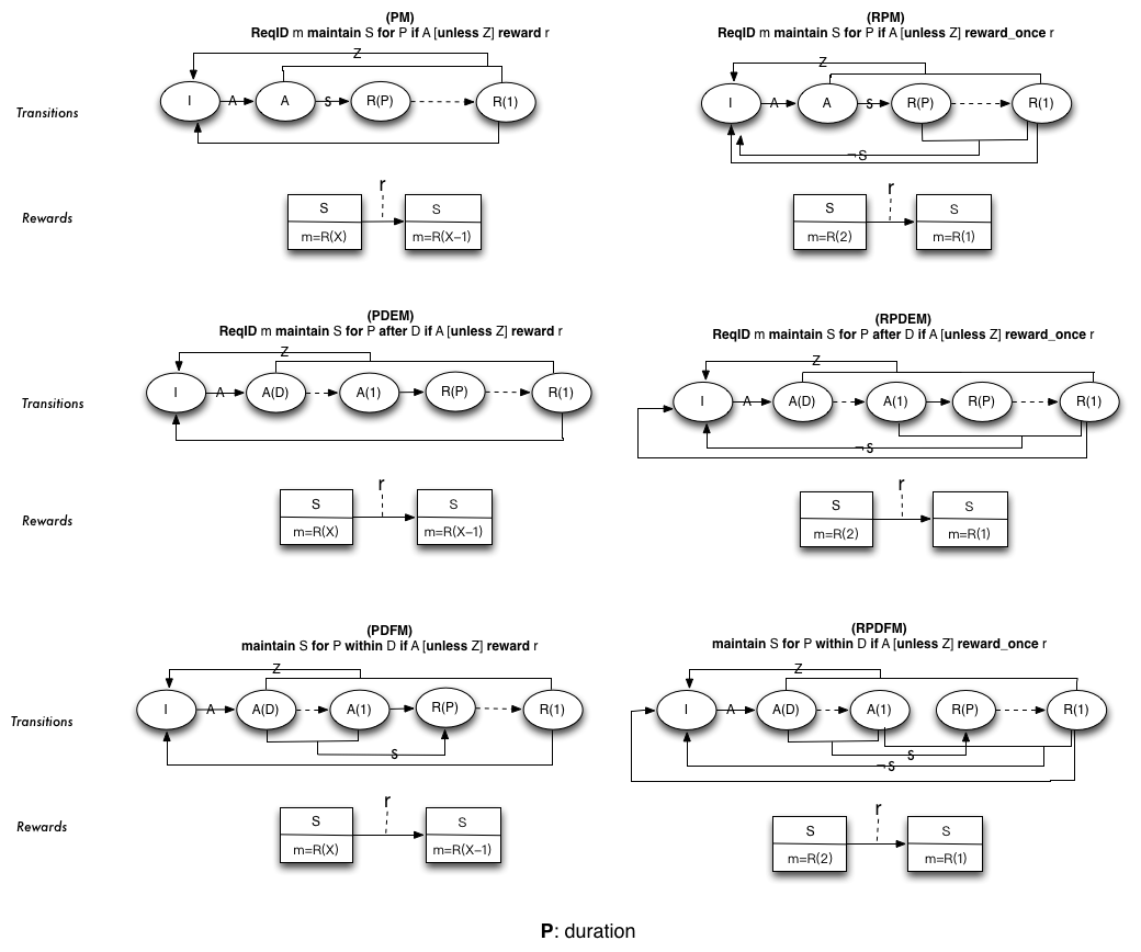
Figure 15: Duration Requirements: Transitions and rewards

References

- [1] M. Salehie and L. Tahvildari, “Self-adaptive software: Landscape and research challenges,” ACM Trans. Auton. Adapt. Syst., vol. 4, no. 2, pp. 1–42, 2009.
- [2] B. H. C. Cheng, R. D. Lemos, H. Giese, P. Inverardi, J. Magee, J. Andersson, B. Becker, N. Bencomo, Y. Brun, B. Cukic, G. D. M. Serugendo, S. Dustdar, A. Finkelstein, C. Gacek, K. Geihs, V. Grassi, G. Karsai, H. M. Kienle, J. Kramer, M. Litoiu, S. Malek, R. Mirandola, H. a. Müller, S. Park, M. Shaw, M. Tichy, M. Tivoli, D. Weyns, J. Whittle, D. Lemos, H. Giese, P. Inverardi, J. Andersson, B. Becker, N. Bencomo, Y. Brun, B. Cukic, G. Di, M. Serugendo, S. Dustdar, A. Finkelstein, C. Gacek, K. Geihs, V. Grassi, G. Karsai, H. M. Kienle, J. Kramer, M. Litoiu, S. Malek, S. Park, M. Shaw, M. Tichy, M. Tivoli, D. Weyns, and J. Whittle, “Software Engineering for Self-Adaptive Systems : A Research Roadmap,” Springer, pp. 1–26, 2009.
- [3] R. D. Lemos, H. Giese, H. a. Müller, M. Shaw, J. Andersson, L. Baresi, B. Becker, N. Bencomo, Y. Brun, B. Cukic, S. Dustdar, G. Engels, K. Geihs, K. M. Goeschka, V. Grassi, P. Inverardi, G. Karsai, J. Kramer, M. Litoiu, J. Magee, S. Malek, S. Mankovskii, R. Mirandola, J. Mylopoulos, O. Nierstrasz, M. Pezzè, C. Prehofer, W. Schäfer, R. Schlichting, D. B. Smith, J. P. Sousa, G. Tamura, L. Tahvildari, M. Norha, T. Vogel, D. Weyns, K. Wong, and J. Wuttke, “Software Engineering for Self-Adaptive Systems : A Second Research Roadmap,” Softw. Eng. Self-Adaptive Syst., no. October 2010, pp. 1–32, 2011.
- [4] N. Esfahani and S. Malek, “Uncertainty in Self-Adaptive Software Systems,” Lect. Notes Comput. Sci., pp. 214–238, 2013.
- [5] G. A. Moreno, J. Cámara, D. Garlan, and B. Schmerl, “Proactive self-adaptation under uncertainty: a probabilistic model checking approach,” ESEC/FSE 2015, pp. 1–12, 2015.
- [6] A. Van Lamsweerde, Requirements engineering : from system goals to UML models to software specifications. John Wiley, 2009.
- [7] P. Zave and M. Jackson, “Four dark corners of requirements engineering,” ACM Trans. Softw. Eng. Methodol., vol. 6, no. 1, pp. 1–30, 1997.
- [8] R. Calinescu, L. Grunske, M. Kwiatkowska, R. Mirandola, and G. Tamburrelli, “Dynamic QoS Management and Optimisation in Service-Based Systems,” TSE, vol. PP, no. 99, p. 1, 2010.
- [9] A. Filieri, G. Tamburrelli, and C. Ghezzi, “Supporting Self-Adaptation via Quantitative Verification and Sensitivity Analysis at Run Time,” IEEE Trans. Softw. Eng., vol. 42, no. 1, pp. 75–99, 2016.
- [10] J. Kephart and D. Chess, “The vision of autonomic computing,” Computer (Long. Beach. Calif)., no. January, pp. 41–50, 2003.
- [11] D. Weyns, “Software Engineering of Self-Adaptive Systems: An Organised Tour and Future Challenges,” Handb. Softw. Eng., pp. 1–41, 2017.
- [12] J. Cámara, G. A. Moreno, and D. Garlan, “Stochastic game analysis and latency awareness for proactive self-adaptation,” SEAMS, no. June, pp. 155–164, 2014.
- [13] J. Cámara, D. Garlan, B. Schmerl, and A. Pandey, “Optimal planning for architecture-based self-adaptation via model checking of stochastic games,” Symp. Appl. Comput., pp. 428–435, 2015.
- [14] J. Cámara, G. A. Moreno, D. Garlan, and B. Schmerl, “Analyzing Latency-Aware Self-Adaptation Using Stochastic Games and Simulations,” ACM Trans. Auton. Adapt. Syst., vol. 10, no. 4, pp. 1–28, 2016.
- [15] M. Kwiatkowska, G. Norman, and D. Parker, “PRISM 4.0: Verification of Probabilistic Real-Time Systems,” in Int. Conf. Comput. Aided Verif., 2011, pp. 585–591.
- [16] F. Bacchus, C. Boutilier, and A. Grove, “Rewarding Behaviors,” in Thirteen. Natl. Conf. Artif. Intell., 1996, pp. 1160–1167.
- [17] C. Boutilier, T. Dean, and S. Hanks, “Decision-Theoretic Planning: Structural Assumptions and Computational Leverage,” J. Artif. Intell. Res., vol. 11, pp. 1–94, 1999.
- [18] P. Sawyer, N. Bencomo, J. Whittle, E. Letie, and A. Finkelstein, “Requirements-aware systems: A research agenda for RE for self-adaptive systems,” RE, pp. 95–103, 2010.
- [19] J. Whittle, P. Sawyer, N. Bencomo, B. H. Cheng, and J. M. Bruel, “RELAX: A language to address uncertainty in self-adaptive systems requirement,” Requir. Eng., vol. 15, no. 2, pp. 177–196, 2010.
- [20] M. Morandini, L. Penserini, A. Perini, and A. Marchetto, “Engineering requirements for adaptive systems,” Requir. Eng., vol. 22, no. 1, pp. 77–103, 2017.
- [21] H. Skubch, “Modelling and Controlling Behaviour of Cooperative Autonomous Mobile Robots,” Ph.D. dissertation, 2012.
- [22] R. E. Fikes and N. J. Nilsson, “STRIPS : A new approach to the Application of theorem proving to problem solving,” vol. 2, no. October, pp. 189–208, 1971.
- [23] D. Mcdermott, M. Ghallab, A. Howe, C. Knoblock, A. Ram, M. Veloso, D. Weld, and D. Wilkins, “PDDL - The Planning Domain Definition Language,” CVC TR-98-003/DCS TR-1165, Yale Center for Computational Vision and Control, Tech. Rep., 1998.
- [24] E. Letier and A. Van Lamsweerde, “Deriving operational software specifications from system goals,” ACM SIGSOFT Softw. Eng. Notes, vol. 27, no. 6, p. 119, 2002.
- [25] Mausam and A. Kolobov, Planning with Markov Decision Processes: An AI Perspective, 2012, vol. 6, no. 1.
- [26] M. L. Littman, T. L. Dean, and L. P. Kaelbling, “On the Complexity of Solving Markov Decision Problems,” Uncertain. Artif. Intell., pp. 394–402, 1995.
- [27] F. Bacchus, C. Boutilier, and A. Grove, “Structured solution methods for non-Markovian decision processes,” AAAI, pp. 112–117, 1997.
- [28] M. Cashmore, M. Fox, D. Long, D. Magazzeni, B. Ridder, A. Carrera, N. Palomeras, N. Hurtos, and M. Carreras, “Rosplan: Planning in the robot operating system.” in ICAPS, 2015, pp. 333–341.
- [29] J. Sun, Y. Liu, J. S. Dong, and J. Pang, “Pat: Towards flexible verification under fairness,” ser. Lecture Notes in Computer Science, vol. 5643. Springer, 2009, pp. 709–714.
- [30] C. Dehnert, S. Junges, J.-P. Katoen, and M. Volk, “A Storm is Coming: A Modern Probabilistic Model Checker,” in Comput. Aided Verif., 2017, vol. 10427, pp. 592–600.
- [31] “PDDL4J library.” [Online]. Available: https://github.com/pellierd/pddl4j
- [32] F. Heidenreich, J. Johannes, S. Karol, M. Seifert, and C. Wende, “Model-Based Language Engineering with EMFText,” 2013, pp. 322–345.
- [33] R. S. Iadine Chades, Guillaume Chapron, Marie-Josee Cros, Frederick Garcia, “Markov Decision Processes Toolbox,” 2017.
- [34] J. Ellson, E. Gansner, L. Koutsofios, S. C. North, and G. Woodhull, “Graphviz - Open Source Graph Drawing Tools,” 2002, pp. 483–484.
- [35] I. Epifani, C. Ghezzi, R. Mirandola, and G. Tamburrelli, “Model Evolution by Run-Time Parameter Adaptation,” Proc. - Int. Conf. Softw. Eng., pp. 111–121, 2009.
- [36] R. Calinescu, Y. Rafiq, K. Johnson, and M. E. Bakır, “Adaptive model learning for continual verification of non-functional properties,” Proc. 5th ACM/SPEC Int. Conf. Perform. Eng. - ICPE ’14, no. May, pp. 87–98, 2014.
- [37] G. Tesauro, “Reinforcement learning in autonomic computing: A manifesto and case studies,” IEEE Internet Computing, vol. 11, 2007.
- [38] A. Lapouchnian, “Goal-oriented requirements engineering: An overview of the current research,” Tech. Rep. 3, 2005.
- [39] A. V. Lamsweerde, Requirements Engineering: From System Goals to UML Models to Software Specifications, 10th ed. Chichester, UK: John Wiley & Sons, 2009.
- [40] E. Yu, “Modelling strategic relationships for process reengineering,” Ph.D. dissertation, University of Toronto, 2011.
- [41] L. Baresi, L. Pasquale, and P. Spoletini, “Fuzzy goals for requirements-driven adaptation,” RE, pp. 125–134, 2010.
- [42] A. Cailliau and A. Van Lamsweerde, “Runtime Monitoring and Resolution of Probabilistic Obstacles to System Goals,” Int. Symp. Softw. Eng. Adapt. Self-Managing Syst., pp. 1–11, 2017.
- [43] D. Garlan, S.-W. Cheng, A.-C. Huang, B. Schmerl, and P. Steenkiste, “Rainbow: Architecture- Based Self-Adaptation with Reusable Infrastructure,” Computer (Long. Beach. Calif)., pp. 46–54, 2004.
- [44] S. W. Cheng and D. Garlan, “Stitch: A language for architecture-based self-adaptation,” J. Syst. Softw., vol. 85, no. 12, pp. 2860–2875, 2012.
- [45] A. Filieri, C. Ghezzi, and G. Tamburrelli, “A formal approach to adaptive software: Continuous assurance of non-functional requirements,” Form. Asp. Comput., vol. 24, no. 2, pp. 163–186, 2012.
- [46] M. U. Iftikhar and D. Weyns, “ActivFORMS: active formal models for self-adaptation,” Proc. 9th Int. Symp. Softw. Eng. Adapt. Self-Managing Syst. - SEAMS 2014, pp. 125–134, 2014.
- [47] N. Esfahani, E. Kouroshfar, and S. Malek, “Taming uncertainty in self-adaptive software,” FSE, pp. 234–244, 2011.
- [48] A. Elkhodary, N. Esfahani, and S. Malek, “FUSION : A Framework for Engineering Self-Tuning Self-Adaptive Software Systems,” FSE, pp. 7–16, 2010.
- [49] N. Bencomo and A. Belaggoun, “Supporting decision-making for self-adaptive systems: From goal models to dynamic decision networks,” REFSQ, vol. 7830 LNCS, pp. 221–236, 2013.
- [50] A. Filieri, H. Hoffmann, and M. Maggio, “Automated design of self-adaptive software with control-theoretical formal guarantees,” in Proc. 36th Int. Conf. Softw. Eng. - ICSE 2014. New York, New York, USA: ACM Press, 2014, pp. 299–310.
- [51] ——, “Automated multi-objective control for self-adaptive software design,” ESEC/FSE 2015, pp. 13–24, 2015.
- [52] S. Shevtsov and D. Weyns, “Keep it SIMPLEX: satisfying multiple goals with guarantees in control-based self-adaptive systems,” FSE, pp. 229–241, 2016.
- [53] A. Filieri, M. Maggio, K. Angelopoulos, N. D’Ippolito, I. Gerostathopoulos, A. B. Hempel, H. Hoffmann, P. Jamshidi, E. Kalyvianaki, C. Klein, F. Krikava, S. Misailovic, A. V. Papadopoulos, S. Ray, A. M. Sharifloo, S. Shevtsov, M. Ujma, and T. Vogel, “Control strategies for self-adaptive software systems,” ACM Trans. Auton. Adapt. Syst., vol. 11, no. 4, 2017.
- [54] R. Calinescu, D. Weyns, S. Gerasimou, M. U. Iftikhar, I. Habli, and T. Kelly, “Engineering Trustworthy Self-Adaptive Software with Dynamic Assurance Cases,” IEEE Trans. Softw. Eng., pp. 1–29, 2017.
- [55] D. Weyns, N. Bencomo, R. Calinescu, J. Cámara, C. Ghezzi, V. Grassi, L. Grunske, P. Inverardi, J.-M. Jezequel, S. Malek, R. Mirandola, M. Mori, and G. Tambrrellii, “Perpetual Assurances for Self-Adaptive Systems,” Softw. Eng. Self-Adaptive Syst. 3, no. 9640, 2017.
- [56] M. U. Iftikhar and D. Weyns, “ActivFORMS: A runtime environment for architecture-based adaptation with guarantees,” Softw. Archit. Work., pp. 278–281, 2017.
- [57] A. Pandey, G. Moreno, J. Cámara, and D. Garlan, “Hybrid Planning for Decision Making in Self-Adaptive Systems,” 10th IEEE Int. Conf. Self-Adaptive Self-Organizing Syst. (SASO 2016), 2016.
- [58] G. A. Moreno, J. Camara, D. Garlan, and B. Schmerl, “Efficient decision-making under uncertainty for proactive self-adaptation,” Proc. - 2016 IEEE Int. Conf. Auton. Comput. ICAC 2016, pp. 147–156, 2016.