Reconfigurable multiport switch in coupled mode devices

Abstract

We consider a coupled mode system where the effective propagation constants of localized modes are amenable to modulation. Starting from an unmodulated system where power transfer is heavily suppressed, we demonstrate that small, periodic modulation of the propagation constants enhance power transfer using a slowly varying envelope approximation for the field mode amplitudes. We calculate an approximate modulation frequency enabling complete transfer between otherwise negligibly coupled elements. The ability to control these modulations by electrical or thermal effects allows for reconfigurable multiport switching. We use an array of coupled silica waveguides and the thermo-optic effect to test our predictions in the telecom C-band. However, this requires a refractive index modulation with period of the order $~{}10^{-3}~{}\mathrm{m}$ and yields total power transfer with a propagation distance of the order of $10^{-1}~{}\mathrm{m}$, which might make it unattractive for integrated photonic applications. Nevertheless, our results are valid for devices described by an equivalent coupled mode matrix for space or time propagation; for example, arrays of microring or terahertz resonators, microwave cavities, radio frequency antennas, or RLC circuits.

I Introduction

Multiport switching is essential in both classical and quantum optics applications. It is useful to route optical signals in photonic devices and provides a technological platform for photon-based programmable quantum computers Matthews et al. (2009); Carolan et al. (2015); Wang et al. (2018). Optical switch design relies on a plethora of physical systems, including micro-electro-mechanical Giles et al. (1999); Borovic et al. (2004); Yano et al. (2005), complementary metal oxide semiconductor Tsybeskov et al. (2009); Rylyakov et al. (2012), and evanescently coupled waveguides. We focus on the latter as it displays a strong similarity with finite dimensional quantum mechanical systems and allows us to exploit optical analogues of quantum mechanical effects Longhi (2009) and abstract symmetries Rodríguez-Lara and Guerrero (2015); Villanueva Vergara and Rodríguez-Lara (2015); Rodríguez-Lara et al. (2018).

In waveguide arrays, switching may be induced by coupling strength modulation while keeping the refractive indices constant. This produces optical analogues, for example, of stimulated Raman adiabatic passage (STIRAP) Longhi (2006); Longhi et al. (2007); Della Valle et al. (2008), where coupling strength modulation occurs along the propagation direction, or optical realizations of $\mathbf{J}_{x}$ Hamiltonians Perez-Leija et al. (2013), where the modulation is constant along the propagation direction but varies from waveguide to waveguide. Other approaches vary the effective refractive indices of individual waveguides while keeping the couplings constant. This produces optical analogues of Anderson localization of light John (1984); De Raedt et al. (1989); Schwartz et al. (2007); Segev et al. (2013); Jaramillo Ávila et al. (2019), where the refractive index of individual waveguides varies randomly, or parity-time symmetry Ruschhaupt et al. (2005); El-Ganainy et al. (2007); Huerta Morales et al. (2016); Nodal Stevens et al. (2018), where refractive indices include gain or loss following a certain structure. Finally, other approaches vary both couplings and refractive indices Rodríguez-Lara et al. (2014a, b); Rodríguez-Walton et al. (2020).

Here, we are interested on the latter and propose a scheme where coupling strengths are constant but vary from waveguide to waveguide following an abstract symmetry plus periodical modulation of individual refractive indices. Our symmetry-based proposal complements grating assisted couplers Marcuse (1987); Huang and Haus (1989); Griffel and Yariv (1991); Alferness et al. (1992); Weisen et al. (2019), where dissimilar waveguides are coupled by resonant periodic variations in the effective refractive index. The coupling allows near complete power transfer between the waveguides. Without the grating, the waveguides would have negligible power transfer due to high effective refractive index differences between them. These gratings can be fixed Marcuse (1987); Huang and Haus (1989) or reconfigurable Alferness et al. (1992). This may also be reminiscent of $\Delta\beta$ switches Kogelnik and Schmidt (1975, 1976); Schmidt and Alferness (1979); Korotky (1986); Findakly and Leonberger (1988), where a switch designed for a given wavelength can work with a different one by adjusting an alternating constant phase shift induced by the electro-optic effect through a series of electrodes.

Our proposal starts from an array where power transfer is negligible due to high refractive index differences between individual waveguides. We use the underlying symmetry and harmonic modulation of refractive indices to induce power transfer in a manner analogous to population inversion due to optical driving in quantum systems Mandel and Wolf (1995). Controlled changes of the refractive index can be induced by electro- Turner (1966); Long et al. (1994) or thermo-optic Gao et al. (2018) effects, for example. The former has applications in building modulators Liu et al. (2015). The latter is widely used to produce controlled phase shifts in directional couplers in quantum photonic circuits Matthews et al. (2009); Carolan et al. (2015); Wang et al. (2018). Electro- and thermo-optic modulation produce small refractive index changes of the order of $10^{-10}$ per volt/meter Turner (1966); Long et al. (1994) and $10^{-5}$ per kelvin Gao et al. (2018), in that order. For such small variations of the refractive index, power transfer, or switching, occurs over long propagation distances. The level of control and the long propagation distances required to produce reconfigurable multiport switching might render our proposal unfeasible for integrated photonic devices. However, we hope that theoretical curiosity and its inherent first principles validity for systems described by coupled mode theory, either in space propagation or time evolution, are enough to motivate the exploration of such an avenue in, for example, microring Liu et al. (2005) or terahertz Preu et al. (2008) resonators, microwave cavities Haus and Huang (1991); Elnaggar et al. (2014, 2015), radio frequency antenna Kim and Ling (2007), or RLC circuits Agarwal et al. (2006).

In the following, first, we present a theoretical model describing an array of waveguides with an underlying $SU(2)$ symmetry where different individual refractive indices strongly limit the power transfer produced by evanescent coupling. Then, we add small, controllable, periodic changes on the refractive index of the waveguides and show that the amplitude and frequency of these changes produce resonant power transfer between the waveguides. We show that it is possible to analytically approximate this power transfer using a slowly varying envelope approximation over long propagation distances. Next, we go beyond the coupled mode theory approximation and use a 2D finite element simulation to demonstrate power transfer between waveguides with our approach. Finally, we discuss the implications and requirements of our proposal.

II Model

Coupled mode theory provides a tractable framework to study light propagation along some spatial or temporal dimension $\zeta$ Snyder (1972); McIntyre and Snyder (1973); Huang (1994); for example, evanescently coupled arrays of waveguides or ring microresonators, in that order. The coupled mode equation,

$$-i\,\frac{\mathrm{d}\vec{\mathcal{E}}(\zeta)}{\mathrm{d}\zeta}=\mathbf{M}(\zeta)\cdot\vec{\mathcal{E}}(\zeta),$$ (1)

describes the dynamics of polarized modes localized within the $d$ elements of the array. The field in the $j$-th element is $\vec{E}_{j}(x,y,\zeta)=\hat{\epsilon}\,\psi(x,y)\,\mathcal{E}_{j}(\zeta)$. There, $\hat{\epsilon}$ gives the polarization and $\psi(x,y)$ gives the spatial mode profile. The $d$-dimensional vector $\vec{\mathcal{E}}(\zeta)$ collects the modal amplitudes $\mathcal{E}_{j}(\zeta)$. The coupled mode matrix $\mathbf{M}(\zeta)$ diagonal and off-diagonal elements contain the effective propagation constants corresponding to each element-localized mode and the coupling between pairs of them, in that order. They may depend on the variable $\zeta$ or not.

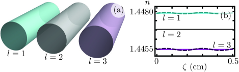
Figure 1: (a) Waveguide array that generates a three-dimensional coupled mode matrix $\mathbf{M}$ and (b) the corresponding refractive indices. The difference in propagation constants, given by $\left[\Delta\beta+f(\zeta)\right]\mathbf{J}_{z}$, is generated by the different refractive indices in (b). The solid lines yield unmodulated propagation constants, $f(\zeta)=0$, while the dashed curves yield a sinusoidal modulation, $f(\zeta)=\delta\sin(\omega\zeta)$. The off-diagonal couplings $2g\,\mathbf{J}_{x}$ are controlled by the separation between the waveguides. The difference between off-diagonal coupling constants in the modulated and unmodulated cases is very small and therefore neglected.

In order to provide multiport switching, we choose an array given in terms of a finite dimensional representation of the angular momentum operators, $\{\hat{J}_{x},\hat{J}_{y},\hat{J}_{z}\}$ Rodríguez-Lara et al. (2014a, b); Villanueva Vergara and Rodríguez-Lara (2015),

$$\mathbf{M}=\beta\,\mathbf{I}+\left[\Delta\beta+f(\zeta)\right]\mathbf{J}_{z}+2g\,\mathbf{J}_{x},$$ (2)

where the propagation constant $\beta$ is common to all elements and the real parameter $\Delta\beta$ characterizes its variation due to the selected $SU(2)$ symmetry. The propagation dependent function $f(\zeta)$ summarizes the effect of controlled, small, periodic variations of individual propagation constants due to changes in refractive indices, resonator lengths, etc, depending on the specific realization. The parameter $g$ characterizes the coupling strength between nearest neighbor element-localized modes. Figure 1 displays an example of a waveguide array that generates the coupled mode matrix $\mathbf{M}$ in the three waveguide case. It is possible to use Wei-Norman factorization to calculate the propagation of modal amplitudes under the dynamics provided by this coupled mode matrix Wei and Norman (1963); Rodríguez-Lara et al. (2018). However, we chose an alternate path of frame transformations for better understanding of the system behavior. In the following, we obviate the baseline constant term $\beta$ as it only induces an overall phase to the modal amplitudes vector.

The base system without periodic variations, $f(\zeta)=0$, constrains power transfer between elements due to the differences on individual effective propagation constants. We can diagonalize the unmodulated coupled mode matrix,

$$\mathbf{M}_{0}=\Delta\beta\,\mathbf{J}_{z}+2g\,\mathbf{J}_{x},$$ (3)

using a rotation of the following form Villanueva Vergara and Rodríguez-Lara (2015),

$$\mathbf{M}_{1}=e^{-i\theta\,\mathbf{J}_{y}}\cdot\mathbf{M}_{0}\cdot e^{i\theta\,\mathbf{J}_{y}}=\Omega\,\mathbf{J}_{z},$$ (4)

in terms of a rotation angle,

$$\tan\theta=-\frac{2g}{\Delta\beta}.$$ (5)

The factor in the diagonal effective coupling matrix, defines an unmodulated device frequency,

$$\Omega=\sqrt{\Delta\beta^{2}+4g^{2}},$$ (6)

such that an array of identical elements, $\Delta\beta=0$, produces complete power transfer between the $l$-th and the $(d-l+1)$-th elements at $\zeta=\pi/\Omega$ Perez-Leija et al. (2013). Differences on the individual refractive indices, $\Delta\beta\neq 0$, suppress power transfer Villanueva Vergara and Rodríguez-Lara (2015).

Under $\zeta$-dependent modulation, this prescription no longer diagonalizes the coupled mode matrix,

$$\mathbf{M}_{2} = e^{-i\theta\,\mathbf{J}_{y}}\cdot\mathbf{M}\cdot e^{i\theta\,\mathbf{J}_{y}}$$ (7)

$$= \left[\Omega+\frac{\Delta\beta\,f(\zeta)}{\Omega}\right]\mathbf{J}_{z}-\left[\frac{2g\,f(\zeta)}{\Omega}\right]\mathbf{J}_{x}.$$

However, we can move to a $\zeta$-dependent frame defined by a rotation $e^{i\omega\,\mathbf{J}_{z}\,\zeta}$ to obtain an effective matrix,

$$\mathbf{M}_{3} = e^{-i\omega\,\mathbf{J}_{z}\,\zeta}\cdot\mathbf{M}_{2}\cdot e^{i\omega\,\mathbf{J}_{z}\,\zeta}-\omega\,\mathbf{J}_{z},$$ (8)

$$= \frac{\Delta\beta\,f(\zeta)}{\Omega}\,\mathbf{J}_{z}+\left(\Omega-\omega\right)\mathbf{J}_{z}$$

$$-\frac{g\,f(\zeta)}{\Omega}\left(\mathbf{J}_{+}\,e^{-i\omega\,\zeta}+\mathbf{J}_{-}\,e^{i\omega\,\zeta}\right),$$

where we used $\mathbf{J}_{x}=\left(\mathbf{J}_{+}+\mathbf{J}_{-}\right)/2$. This suggests the use of harmonic modulation,

$$f(\zeta)=\delta\sin(\omega\,\zeta),$$ (9)

to induce fast and slow frequencies in the system,

$$\mathbf{M}_{3} = \frac{\delta\,\Delta\beta}{\Omega}\sin(\omega\,\zeta)\,\mathbf{J}_{z}+\left(\Omega-\omega\right)\mathbf{J}_{z}$$ (10)

$$+\frac{i\delta g}{2\Omega}\!\left[\left(1-e^{-i2\omega\zeta}\right)\mathbf{J}_{+}-\left(1-e^{i2\omega\zeta}\right)\mathbf{J}_{-}\right]\!\!.$$

Our system now includes five effective frequencies: $\delta\,\Delta\beta/\Omega$, $(\Omega-\omega)$, $\delta\,g/(2\Omega)$, $\omega$ and $2\omega$. Control of the individual propagation constants by electro- or thermo-optic effects usually provides a small amplitude modulation parameter compared to the coupling strength and propagation constant difference, $\delta<g$ and $\delta<\Delta\beta$. In consequence, it is smaller than the unmodulated device frequency $\delta\ll\Omega$. This leads to the following fact. Unless we choose a modulation frequency close to the unmodulated device frequency, $\omega\sim\Omega$, the first and third terms on the right hand of Eq. (10) may become irrelevant. Furthermore, we can set them to be similar $\delta\,\Delta\beta/\Omega\sim\left(\Omega-\omega\right)\sim\delta\,g/(2\Omega)$, leading to an ordered relation $\delta\,\Delta\beta/\Omega\sim\left(\Omega-\omega\right)\sim\delta\,g/(2\Omega)\ll\omega<2\omega$. This suggests using a rotating wave approximation (RWA) to neglect fast oscillating terms Allen and Eberly (1975),

$$\mathbf{M}_{3}\sim\left(\Omega-\omega\right)\mathbf{J}_{z}-\left(\frac{\delta\,g}{\Omega}\right)\mathbf{J}_{y},$$ (11)

and realize that we can diagonalize this effective coupled mode matrix by using a rotation along $\mathbf{J}_{x}$,

$$e^{-i\phi\,\mathbf{J}_{x}}\cdot\mathbf{M}_{3}\cdot e^{i\phi\,\mathbf{J}_{x}}=\Omega_{S}\,\mathbf{J}_{z},$$ (12)

where the rotation angle $\phi$ fulfills the relation,

$$\tan\phi=-\frac{\delta\,g}{\Omega\left(\Omega-\omega\right)}.$$ (13)

This leads to an effective diagonal coupled mode matrix with a device frequency,

$$\Omega_{S}=\sqrt{(\Omega-\omega)^{2}+\left(\frac{\delta g}{\Omega}\right)^{2}}\ll\Omega,\omega,$$ (14)

slower than the frequencies of unmodulated device $\Omega$ and the thermal- or electro-optic modulation $\omega$. The modulated device provides complete power transfer between the $l$-th and the $(d-l+1)$-th waveguides for modulation frequency equal to the unmodulated device frequency, $\omega=\Omega$, at the approximate value $\zeta=\Omega\,\pi/(\delta\,g)$.

The rotating wave approximation, made by neglecting the fast oscillating terms with frequencies $\omega$ and $2\omega$, is equivalent to calculating the dynamics under a slowly varying envelope approximation (SVEA) of the modal field amplitude vector. This can be seen in the solution for the modal amplitudes vector,

$$\vec{\mathcal{E}}(\zeta) \sim e^{i\beta\zeta}\cdot e^{i\theta\,\mathbf{J}_{y}}\cdot e^{i\omega\,\mathbf{J}_{z}\,\zeta}\cdot e^{i\phi\,\mathbf{J}_{x}}\cdot e^{i\Omega_{S}\,\mathbf{J}_{z}\,\zeta}\cdot e^{-i\phi\,\mathbf{J}_{x}}\cdot$$ (15)

$$e^{-i\omega\,\mathbf{J}_{z}\,\zeta}\cdot e^{-i\theta\,\mathbf{J}_{y}}\cdot\vec{\mathcal{E}}(0),$$

where the initial state of the system is $\vec{\mathcal{E}}(0)$. It is straightforward to identify the $\zeta$-dependent terms responsible for the slowly varying envelope $e^{\pm i\Omega_{S}\,\mathbf{J}_{z}\,\zeta}$ and the fast modulation $e^{\pm i\omega\,\mathbf{J}_{z}\,\zeta}$ behaviors.

III Telecom C-band example

Let us consider a realization for telecom C-band, $\lambda=1\,550~{}\mathrm{nm}$, using cylindrical fused silica waveguides. Since all waveguides must have different refractive indices, we use core refractive indices in the range $[1.445\,95,1.447\,90]$ and a cladding index of $1.444\,00$ consistent with laser writing experiments Eaton et al. (2011). We choose a core radius of $4.5~{}\mu\mathrm{m}$ to support a single LP₀₁ mode in each waveguide. For a realization with $d$ waveguides, the data above determines $\beta$ and $\Delta\beta$, fixing the localized single mode propagation constants for each waveguide. The corresponding individual core refractive indices can be numerically calculated from these. The next step is to find a reference value for the coupling parameter $g$. Doing so fixes the couplings between pairs of neighboring waveguides. The corresponding waveguide separations can be numerically extracted from this.

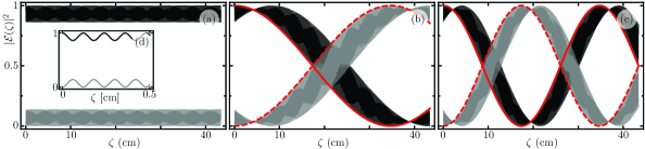
Figure 2: Squared field amplitude as a function of the propagation distance (a) with no refractive index modulation, (b) weak refractive index modulation, and (c) strong refractive index modulation. Inset (d) displays the squared field amplitude on a short propagation distance with limited power transfer oscillations. Black and gray curves display squared amplitudes within waveguides $l=1$ and $l=2$, respectively, provided by numerically solving the $\zeta$-dependent coupled matrix. Red solid and dashed curves are the analytic approximate slowly varying envelopes.

Let us start with the simplest case, two waveguides described by the parameter set $\{\beta,\Delta\beta,g\}=\{5.857\,32\times 10^{6},4\,872.24,974.447\}~{}\mathrm{rad}/\mathrm{m}$. The corresponding center-to-center core separation is $11.02~{}\mu\mathrm{m}$. We will assume thermo-optic effect as the drive behind periodic core refractive index modulation. Silica first-order thermo-optic coefficient $1.090\times 10^{-5}~{}\mathrm{K}^{-1}$ and temperature contrast of the order of 5$~{}\mathrm{K}$ between the cooler and the hotter parts of the waveguides yields an amplitude of the propagation constant modulation of the order $\delta=97.444\,7~{}\mathrm{rad}/\mathrm{m}$. Figure 2(a) displays the suppressed power-transfer between the two waveguides with no refractive index modulation. Figure 2(b) displays power transfer when the modulation period is on resonance, $\omega=\Omega$, and has an intermediate amplitude $\delta=0.05~{}g=48.722\,4~{}\mathrm{rad}/\mathrm{m}$. There, the distance for near complete power transfer is $\Omega\,\pi/(\delta\,g)=34.72~{}\mathrm{cm}$. Figure 2(c) displays power transfer on resonance with stronger modulation $\delta=0.1~{}g=97.444\,7~{}\mathrm{rad}/\mathrm{m}$ where the distance for near complete power transfer is $\Omega\,\pi/(\delta\,g)=17.36~{}\mathrm{cm}$. As the modulation amplitude increases, the near complete transfer length decreases. The results in gray and black are numerical solutions for the full $\zeta$-dependent system without approximations, Eq. (2). The solid and dashed red lines are the evolution of just the approximate slowly varying envelope solution.

Increasing the number of waveguides in the array allows for reconfigurable switching between more ports. As an example, we focus on the three waveguide case exemplified in Fig. 1, which yields a parameter set $\{\beta,\Delta\beta,g\}=\{5.857\,32\times 10^{6},2\,436.12,487.224\}~{}\mathrm{rad}/\mathrm{m}$. The core refractive indices are now modulated to $\{n_{1},n_{2},n_{3}\}=\{1.447\,90,1.447\,02,1.445\,95\}$ and their separation distances $\{d_{12},d_{23}\}=\{12.44,12.19\}~{}\mu\mathrm{m}$ are not equal to maintain a constant effective coupling with different refractive indices. The thermal contrast of 5$~{}\mathrm{K}$ yields a modulation amplitude $\delta=0.1~{}g=48.722\,4~{}\mathrm{rad}/\mathrm{m}$. The amplitude of the modulation $\delta$ is smaller than the one in the two-waveguide case but the maximum absolute change of individual core refractive indices are the same. Figure 3 displays the squared field amplitude when light impinges on the central waveguide, $l=2$. Power transfer from the central core to the external ones occurs at $\Omega\,\pi/(2g\,\delta)=17.36~{}\mathrm{cm}$. This plot contains coupled mode results, where the transversal information is obtained multiplying the coupled mode squared field amplitude results with the mode profiles of the waveguides, which are readily obtained with finite element analysis for the modes.

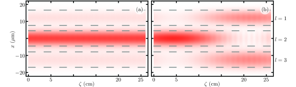
Figure 3: Squared field amplitude of the electric field in a coupled mode theory calculation with cylindrical waveguides. Here, light is impinged on the middle waveguide, $l=2$, (a) with and (b) without resonant, $\omega=\Omega$, refractive index modulation. The vertical axis, $x$, gives the separation between the waveguides and the horizontal axis, $\zeta$, is the propagation distance. More details in text.

To insure the validity of our proposal, we go beyond the coupled mode theory approximation, and use a finite element simulation with COMSOL. In order to keep our simulation tractable in a standard workstation we restrict ourselves to two waveguides in a 2D simulation. This restriction is necessary due to the long propagation distances, of tens of centimeters. Our simulation describes planar silica waveguides in the telecom C-band with $9~{}\mu\mathrm{m}$ thickness and $13.45~{}\mu\mathrm{m}$ center-to-center separation, see Fig. 4. Their refractive indices are $1.44790$ and $1.44722$ for each of the upper and lower waveguides in Fig. 4(a) and (b), additionally the cladding and inter-waveguide refractive index is $1.44400$. The unmodulated case, Fig. 4(a), displays limited power transfer between the waveguides. In contrast, the modulated case, Fig. 4(b), displays almost complete power transfer between the waveguides due to small refractive index changes along the propagation direction. The modulation has spatial frequency $\omega=2624.32~{}\mathrm{rad}/\mathrm{m}$ and amplitude of $3\times 10^{-5}$, consistent with temperature differences $5~{}\mathrm{C}$ between the hottest and coldest parts of a waveguide.

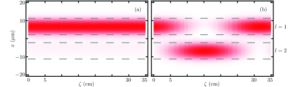
Figure 4: Squared field amplitude of the electric field in a 2D finite element simulation. Here, light is impinged on the upper waveguide, $l=1$, (a) with and (b) without resonant, $\omega=\Omega$, refractive index modulation. The vertical axis, $x$, gives the separation between the waveguides and the horizontal axis, $\zeta$, is the propagation distance. More details in text.

IV Conclusions

We demonstrated reconfigurable power transfer in nearest neighbor coupled mode systems by using periodic modulation of the localized modes effective propagation constant. In our proposal, an unmodulated system, where power transfer is heavily suppressed due to differences between the localized mode propagation constants, can show near complete power transfer if we introduce harmonic modulation with the correct frequency. We provide an approximate effective power transfer frequency using the equivalent of a slowly varying envelope approximation for the modal field amplitudes. In our devices, the required modulation frequency is wavelength dependent through propagation constants and waveguide couplings. Therefore, unlike $\Delta\beta$ switches Kogelnik and Schmidt (1975, 1976); Schmidt and Alferness (1979); Korotky (1986); Findakly and Leonberger (1988); Tsukada (1977); Molter-Orr and Haus (1985), to operate our device at different wavelengths it becomes necessary to adjust not only the modulation amplitude, but also the modulation frequency.

As a practical example, we work with fused silica waveguides and their first-order thermo-optic response in the telecom C-band. We present results using coupled mode theory and 2D finite element simulations. Here, the modulation amplitudes are small and the distances for power transfer become large, of the order of tens of centimeters. While proving the first principles validity of our proposal, this may not be feasible for photonic integrated devices. However, our results are valid for coupled mode systems, propagating in space or time, where the equivalent of localized propagation constants can be modulated in a controlled manner by electrical or thermal effects. For example, microring resonators or terahertz resonators, microwave cavities, radio frequency antennas, or RLC circuits.

References

- Matthews et al. (2009) J. C. F. Matthews, A. Politi, A. Stefanov, and J. L. O’Brien, “Manipulation of multiphoton entanglement in waveguide quantum circuits,” Nat. Photonics 3, 346–350 (2009), arXiv:0911.1257 [quant-ph] .
- Carolan et al. (2015) J. Carolan, C. Harrold, C. Sparrow, E. Martín-López, N. J. Russell, J. W. Silverstone, P. J. Shadbolt, N. Matsuda, M. Oguma, M. Itoh, G. D. Marshall, M. G. Thompson, J. C. F. Matthews, T. Hashimoto, J. L. O’Brien, and A. Laing, “Universal linear optics,” Science 349, 711–716 (2015), arXiv:1505.01182 [quant-ph] .
- Wang et al. (2018) J. Wang, S. Paesani, Y. Ding, R. Santagati, P. Skrzypczyk, A. Salavrakos, J. Tura, R. Augusiak, L. Mančinska, D. Bacco, D. Bonneau, J. W. Silverstone, O. Gong, A. Acín, K. Rottwitt, L. K. Oxenløwe, J. L. O’Brien, A. Laing, and M. G. Thompson, “Multidimensional quantum entanglement with large-scale integrated optics,” Science 360, 285–291 (2018), arXiv:1803.04449 [quant-ph] .
- Giles et al. (1999) C. R. Giles, V. Aksyuk, B. Barber, R. Ruel, L. Stulz, and D. Bishop, “A silicon MEMS optical switch attenuator and its use in lightwave subsystems,” IEEE J. Sel. Top. Quant. 5, 18–25 (1999).
- Borovic et al. (2004) B. Borovic, C. Hong, A. Q. Liu, L. Xie, and F. L. Lewis, “Control of a MEMS optical switch,” in 2004 43rd IEEE Conference on Decision and Control (CDC), Vol. 3 (2004) pp. 3039–3044.
- Yano et al. (2005) M. Yano, F. Yamagishi, and T. Tsuda, “Optical MEMS for photonic switching-compact and stable optical crossconnect switches for simple, fast, and flexible wavelength applications in recent photonic networks,” IEEE J. Sel. Top. Quant. 11, 383–394 (2005).
- Tsybeskov et al. (2009) L. Tsybeskov, D. J. Lockwood, and M. Ichikawa, “Silicon photonics: CMOS going optical [scanning the issue],” Proc. IEEE 97, 1161–1165 (2009).
- Rylyakov et al. (2012) A. V. Rylyakov, C. L. Schow, B. G. Lee, W. M. J. Green, S. Assefa, F. E. Doany, M. Yang, J. Van Campenhout, C. V. Jahnes, J. A. Kash, and Y. A. Vlasov, “Silicon photonic switches hybrid-integrated with CMOS drivers,” IEEE J. Solid-St. Circ. 47, 345–354 (2012).
- Longhi (2009) S. Longhi, “Quantum-optical analogies using photonic structures,” Laser Photonics Rev. 3, 243–261 (2009).
- Rodríguez-Lara and Guerrero (2015) B. M. Rodríguez-Lara and J. Guerrero, “Optical finite representation of the Lorentz group,” Opt. Lett. 40, 5682–5685 (2015), arXiv:1508.05419 [physics.optics] .
- Villanueva Vergara and Rodríguez-Lara (2015) L. Villanueva Vergara and B. M. Rodríguez-Lara, “Gilmore-Perelomov symmetry based approach to photonic lattices,” Opt. Express 23, 22836–22846 (2015), arXiv:1506.02062 [physics.optics] .
- Rodríguez-Lara et al. (2018) B. M. Rodríguez-Lara, R. El-Ganainy, and J. Guerrero, “Symmetry in optics and photonics: a group theory approach,” Sci. Bull. 63, 244–251 (2018), arXiv:1803.00121 [physics.optics] .
- Longhi (2006) S. Longhi, “Adiabatic passage of light in coupled optical waveguides,” Phys. Rev. E 73, 026607 (2006).
- Longhi et al. (2007) S. Longhi, G. Della Valle, M. Ornigotti, and P. Laporta, “Coherent tunneling by adiabatic passage in an optical waveguide system,” Phys. Rev. B 76, 201101(R) (2007), arXiv:0709.3050 [cond-mat.other] .
- Della Valle et al. (2008) G. Della Valle, M. Ornigotti, T. Toney Fernandez, P. Laporta, S. Longhi, A. Coppa, and V. Foglietti, “Adiabatic light transfer via dressed states in optical waveguide arrays,” Appl. Phys. Lett. 92, 011106 (2008).
- Perez-Leija et al. (2013) A. Perez-Leija, R. Keil, A. Kay, H. Moya-Cessa, S. Nolte, L.-C. Kwek, B. M. Rodríguez-Lara, A. Szameit, and D. N. Christodoulides, “Coherent quantum transport in photonic lattices,” Phys. Rev. A 87, 012309 (2013), arXiv:1207.6080 [quant-ph] .
- John (1984) S. John, “Electromagnetic absorption in a disordered medium near a photon mobility edge,” Phys. Rev. Lett. 53, 2169–2172 (1984).
- De Raedt et al. (1989) H. De Raedt, A. Lagendijk, and P. de Vries, “Transverse localization of light,” Phys. Rev. Lett. 62, 47–50 (1989).
- Schwartz et al. (2007) T. Schwartz, G. Bartal, S. Fishman, and M. Segev, “Transport and Anderson localization in disordered two-dimensional photonic lattices,” Nature 446, 52–55 (2007).
- Segev et al. (2013) M. Segev, Y. Silberberg, and D. N. Christodoulides, “Anderson localization of light,” Nat. Photonics 7, 197–204 (2013).
- Jaramillo Ávila et al. (2019) B. Jaramillo Ávila, J. M. Torres, R. de J. León-Montiel, and B. M. Rodríguez-Lara, “Optimal crosstalk suppression in multicore fibers,” Sci. Rep. 9, 15737 (2019), arXiv:1905.09416 [physics.optics] .
- Ruschhaupt et al. (2005) A. Ruschhaupt, F. Delgado, and J. G. Muga, “Physical realization of PT-symmetric potential scattering in a planar slab waveguide,” J. Phys. A: Math. Gen 38, L171–L176 (2005).
- El-Ganainy et al. (2007) R. El-Ganainy, K. G. Makris, D. N. Christodoulides, and Z. H. Musslimani, “Theory of coupled optical PT-symmetric structures,” Opt. Lett. 32, 2632–2634 (2007).
- Huerta Morales et al. (2016) J. D. Huerta Morales, J. Guerrero, S. López-Aguayo, and B. M. Rodríguez-Lara, “Revisiting the optical PT-symmetric dimer,” Symmetry 8, 83 (2016), arXiv:1607.02782 [physics.optics] .
- Nodal Stevens et al. (2018) D. J. Nodal Stevens, B. Jaramillo Ávila, and B. M. Rodríguez-Lara, “Necklaces of PT-symmetric dimers,” Photon. Res. 6, A31–A37 (2018), arXiv:1709.00498 [physics.optics] .
- Rodríguez-Lara et al. (2014a) B. M. Rodríguez-Lara, P. Aleahmad, H. M. Moya-Cessa, and D. N. Christodoulides, “Ermakov-Lewis symmetry in photonic lattices,” Opt. Lett. 39, 2083–2085 (2014a).
- Rodríguez-Lara et al. (2014b) B. M. Rodríguez-Lara, H. M. Moya-Cessa, and D. N. Christodoulides, “Propagation and perfect transmission in three-waveguide axially varying couplers,” Phys. Rev. A 89, 013802 (2014b), arXiv:1310.4754 [physics.optics] .
- Rodríguez-Walton et al. (2020) S. Rodríguez-Walton, B. Jaramillo Ávila, and B. M. Rodríguez-Lara, “Optical non-Hermitian para-Fermi oscillators,” Phys. Rev. A 101, 043840 (2020), arXiv:1911.11044 [physics.optics] .
- Marcuse (1987) D. Marcuse, “Directional couplers made of nonidentical asymmetric slabs. Part II: Grating-assisted couplers,” J. Lightwave Technol. 5, 268–273 (1987).
- Huang and Haus (1989) W. Huang and H. A. Haus, “Power exchange in grating-assisted couplers,” J. Lightwave Technol. 7, 920–924 (1989).
- Griffel and Yariv (1991) G. Griffel and A. Yariv, “Frequency response and tunability of grating-assisted directional couplers,” IEEE J. Quantum Electron. 27, 1115–1118 (1991).
- Alferness et al. (1992) R. C. Alferness, L. L. Buhl, U. Koren, B. I. Miller, M. G. Young, T. L. Koch, C. A. Burrus, and G. Raybon, “Broadly tunable InGaAsP/InP buried rib waveguide vertical coupler filter,” Appl. Phys. Lett. 60, 980–982 (1992).
- Weisen et al. (2019) M. J. Weisen, M. T. Posner, J. C. Gates, C. B. E. Gawith, P. G. R. Smith, and P. Horak, “Low-loss wavelength-selective integrated waveguide coupler based on tilted Bragg gratings,” J. Opt. Soc. Am. B 36, 1783–1791 (2019).
- Kogelnik and Schmidt (1975) H. W. Kogelnik and R. V. Schmidt, U.S. Patent No. 4012113A (1975).
- Kogelnik and Schmidt (1976) H. Kogelnik and R. Schmidt, “Switched directional couplers with alternating ,” IEEE J. Quantum Elect. 12, 396–401 (1976).
- Schmidt and Alferness (1979) R. Schmidt and R. Alferness, “Directional coupler switches, modulators, and filters using alternating techniques,” IEEE T. Circuits Syst. 26, 1099–1108 (1979).
- Korotky (1986) S. Korotky, “Three-space representation of phase-mismatch switching in coupled two-state optical systems,” IEEE J. Quantum Elect. 22, 952–958 (1986).
- Findakly and Leonberger (1988) T. K. Findakly and F. J. Leonberger, “On the crosstalk of reversed delta beta directional coupler switches,” J. Lightwave Technol. 6, 36–40 (1988).
- Mandel and Wolf (1995) L. Mandel and E. Wolf, Optical Coherence and Quantum Optics (Cambridge University Press, 1995).
- Turner (1966) E. H. Turner, “High‐frequency electro-optic coefficients of lithium niobate,” Appl. Phys. Lett. 8, 303–304 (1966).
- Long et al. (1994) X-C. Long, R. A. Myers, and S. R. J. Brueck, “Measurement of the linear electro-optic coefficient in poled amorphous silica,” Opt. Lett. 19, 1819–1821 (1994).
- Gao et al. (2018) H. Gao, Y. Jiang, Y. Cui, L. Zhang, J. Jia, and L. Jiang, “Investigation on the thermo-optic coefficient of silica fiber within a wide temperature range,” J. Lightwave Technol. 36, 5881–5886 (2018).
- Liu et al. (2015) K. Liu, C. R. Ye, S. Khan, and V. J. Sorger, “Review and perspective on ultrafast wavelength-size electro-optic modulators,” Laser Photonics Rev. 9, 172–194 (2015).
- Liu et al. (2005) Y. Liu, T. Chang, and A. E. Craig, “Coupled mode theory for modeling microring resonators,” Opt. Eng. 44, 1–6 (2005).
- Preu et al. (2008) S. Preu, H. G. L. Schwefel, S. Malzer, G. H. Döhler, L. J. Wang, M. Hanson, J. D. Zimmerman, and A. C. Gossard, “Coupled whispering gallery mode resonators in the Terahertz frequency range,” Opt. Express 16, 7336–7343 (2008).
- Haus and Huang (1991) H. A. Haus and W. Huang, “Coupled-mode theory,” Proc. IEEE 79, 1505–1518 (1991).
- Elnaggar et al. (2014) S. Y. Elnaggar, R. Tervo, and S. M. Mattar, “Coupled modes, frequencies and fields of a dielectric resonator and a cavity using coupled mode theory,” J. Magn. Reson. 238, 1–7 (2014).
- Elnaggar et al. (2015) S. Y. Elnaggar, R. J. Tervo, and S. M. Mattar, “Energy coupled mode theory for electromagnetic resonators,” IEEE T. Microw. Theory 63, 2115–2123 (2015), arXiv:1305.6085 [cond-mat.other] .
- Kim and Ling (2007) Y. Kim and H. Ling, “Investigation of coupled mode behaviour of electrically small meander antennas,” Electron. Lett. 43, 1250–1252 (2007).
- Agarwal et al. (2006) K. Agarwal, D. Sylvester, and D. Blaauw, “Modeling and analysis of crosstalk noise in coupled RLC interconnects,” IEEE T. Comput. Aid. D. 25, 892–901 (2006).
- Snyder (1972) A. W. Snyder, “Coupled-mode theory for optical fibers,” J. Opt. Soc. Am. 62, 1267–1277 (1972).
- McIntyre and Snyder (1973) P. D. McIntyre and A. W. Snyder, “Power transfer between optical fibers,” J. Opt. Soc. Am. 63, 1518–1527 (1973).
- Huang (1994) W.-P. Huang, “Coupled-mode theory for optical waveguides: an overview,” J. Opt. Soc. Am. A 11, 963–983 (1994).
- Wei and Norman (1963) J. Wei and E. Norman, “Lie algebraic solution of linear differential equations,” J. Math. Phys. 4, 575–581 (1963).
- Allen and Eberly (1975) L. Allen and J. H. Eberly, Optical resonance and two-level atoms (Wiley, 1975).
- Eaton et al. (2011) S. M. Eaton, M. L. Ng, R. Osellame, and P. R. Herman, “High refractive index contrast in fused silica waveguides by tightly focused, high-repetition rate femtosecond laser,” J. Non-Cryst. Solids 357, 2387–2391 (2011).
- Tsukada (1977) N. Tsukada, “Modification of the coupling coefficient by periodic modulation of the propagation constants,” Opt. Commun. 22, 113–115 (1977).
- Molter-Orr and Haus (1985) L. A. Molter-Orr and H. A. Haus, “Multiple coupled waveguide switches using alternating phase mismatch,” Appl. Opt. 24, 1260–1264 (1985).