New constraints on the structure of the nuclear stellar cluster of the Milky Way from star counts and MIR imaging

Abstract

Context. The Milky Way nuclear star cluster (MWNSC) is a crucial laboratory for studying the galactic nuclei of other galaxies, but its properties have not been determined unambiguously until now.

Aims. We aim to study the size and spatial structure of the MWNSC.

Methods. This study uses data and methods that address potential shortcomings of previous studies on the topic. We use $0.2^{\prime\prime}$ angular resolution $K_{s}$ data to create a stellar density map in the central $86.4$pc x $21$pc at the Galactic center. We include data from selected adaptive-optics-assisted images obtained for the inner parsecs. In addition, we use IRAC/Spitzer mid-infrared (MIR) images. We model the Galactic bulge and the nuclear stellar disk in order to subtract them from the MWNSC. Finally, we fit a Sérsic model to the MWNSC and investigate its symmetry.

Results. Our results are consistent with previous work. The MWNSC is flattened with an axis ratio of $q=0.71\pm 0.10$, an effective radius of $R_{e}=(5.1\pm 1.0)$ pc, and a Sérsic index of $n=2.2\pm 0.7$. Its major axis may be tilted out of the Galactic plane by up to $-10$ degrees. The distribution of the giants brighter than the Red Clump (RC) is found to be significantly flatter than the distribution of the faint stars. We investigate the 3D structure of the central stellar cusp using our results on the MWNSC structure on large scales to constrain the deprojection of the measured stellar surface number density, obtaining a value of the 3D inner power law of $\gamma=1.38\pm 0.06_{sys}\pm 0.01_{stat}$.

Conclusions. The MWNSC shares its main properties with other extragalactic NSCs found in spiral galaxies. The differences in the structure between bright giants and RC stars might be related to the existence of not completely mixed populations of different ages. This may hint at recent growth of the MWNSC through star formation or cluster accretion.

1 Introduction

Nuclear stellar clusters (NSCs) are the densest and most massive star clusters in the universe, with half-light radii of $\sim 2-8$ pc and masses of $\sim 10^{6}-10^{7}$M_⊙ (Böker et al. 2002, 2004; Walcher et al. 2005; Côté et al. 2006; Georgiev & Böker 2014). They follow similar scaling relations to their host galaxies in a similar way to super massive black holes (SMBHs), suggesting a common formation mechanism of NSCs and SMBHs closely linked to galaxy evolution. The formation mechanisms of NSCs are still debated. There are two formation scenarios: infall and subsequent merging of star clusters (e.g., Tremaine et al. 1975; Antonini 2013, 2014; Arca-Sedda & Capuzzo-Dolcetta 2014) and in situ formation of stars at the center of a galaxy (e.g., Milosavljević & Merritt 2001; McLaughlin et al. 2006; Brown et al. 2018). To bring some clarity to this topic we need to study the structure, stellar populations, and kinematics of NSCs. The main limitation for detailed studies of NSCs is their compactness, which makes characterisation of their resolved structure challenging for galaxies at large distances.

However, the center of the Milky Way is located at only $\sim 8$ kpc from Earth (Ghez et al. 2008; Gillessen et al. 2009; Gravity Collaboration et al. 2018). It has a $4\times 10^{6}$ M_⊙ (e.g., Boehle et al. 2016; Gillessen et al. 2017; Gravity Collaboration et al. 2018) massive black hole, Sagittarius A* (Sgr A*), surrounded by a $\sim$ $2.5\times 10^{7}$ M_⊙ nuclear star cluster (Schödel et al. 2014a, b; Feldmeier et al. 2014; Chatzopoulos et al. 2015; Feldmeier-Krause et al. 2017) with a half-light radius or effective radius of $\sim 4.2-7$ pc (Schödel et al. 2014a, b; Fritz et al. 2016). The MWNSC was discovered by Becklin & Neugebauer (1968) as a dense stellar structure with a diameter of a few arcminutes and a mass of a few $10^{7}$ M_⊙. It lies embedded within the nuclear stellar disk (NSD), a flat disk-like structure with a radius of $230$ pc and scale height of $\sim 45$ pc (Launhardt et al. 2002). The MWNSC is the only galactic nucleus where we can resolve the stars observationally on scales of about 2 milliparsecs (mpc), assuming diffraction-limited observations at about $2\,\mu$m with an 8-10m telescope. It is therefore a unique test system to study NSCs and explore the transition regimen between SMBH-dominated or NSC-dominated galaxy cores (Graham & Spitler 2009; Neumayer & Walcher 2012).

Although the MWNSC is so close to us, studies of this cluster must overcome various difficulties. Surrounded by miscellaneous components, such as the Galactic bulge (GB), the NSD, and the Galactic disk (GD), it is a challenge to isolate. The extreme extinction ($A_{v}\geq 30$, $A_{k}\sim 3$) toward the GC (e.g., Nishiyama et al. 2009; Schödel et al. 2010; Fritz et al. 2011) means that it can only be observed at infrared wavelengths, and the strong source crowding requires us to use the highest angular resolution possible. Moreover, the NSC presents a complex formation history (see Pfuhl et al. 2011, and references therein). The observed ages of the stars range from $\sim 12$ Gyr to a few million years. In addition, due to observational difficulties, the typical spectroscopic completeness reaches only around $K_{S}=15.5$ stars, currently limiting any direct spectroscopic measurements to at most a few hundred stars (Do et al. 2009; Bartko et al. 2010; Do et al. 2015; Støstad et al. 2015; Feldmeier-Krause et al. 2015).

The purpose of the present paper is to systematically study the size and spatial structure of the NSC of our Galaxy, building on the works of Schödel et al. (2014a) and Fritz et al. (2014, 2016) but using new and different data, in particular high-angular-resolution near-infrared (NIR) imaging on scales of several tens of parsecs. Schödel et al. (2014a) used data in the central $200$ pc from Spitzer/IRAC data at $3.6\mu$m and $4.5\mu$m with an angular resolution of $2^{\prime\prime}$ that are affected by strong diffuse emission from the mini-spiral and the presence of a few extremely bright sources (e.g., IRS1W or IRS7). The other comparable study is by Fritz et al. (2016), who used three different data sets: data from the adaptive-optics-assisted NIR camera NACO/CONICA (NACO) at the ESO Very Large Telescope (VLT) in the central $20^{\prime\prime}$ ($0.8$ pc) with an angular resolution of $\sim 0.08^{\prime\prime}$; data from the Hubble Space Telescope (HST) Wide Field Camera 3 (WFC3)/IR in the central $68^{\prime\prime}$($2.72$ pc), with angular resolution of $0.15^{\prime\prime}$; and VISTA Variables in the Via Lactea data obtained with VISTA InfraRed CAMera (VIRCAM) in the central $2000^{\prime\prime}$($80$ pc), with an angular resolution of $1.0^{\prime\prime}$.

We use a field of view (FOV) of $86$ pc x $20.2$ pc and we use two different data sets: high resolution data with a point spread function (PSF) of $0.2^{\prime\prime}$ full width at half maximum (FWHM) from the GALACTICNUCLEUS survey (Nogueras-Lara et al. 2018a, 2019a) and even higher resolution data ($0.05^{\prime\prime}$) from Gallego-Cano et al. (2018) for the inner parsecs, the most crowded region near Sgr A*. Moreover, we use a larger field from Nishiyama et al. (2013) of the central $\sim 860$ pc x $280$ pc of our Galaxy to explicitly take into account the influence of the different Galactic components that appear superposed on the line-of-sight toward the NSC. One novel aspect of this work is that we use a GB model to minimize the bias of the GB on the measured properties of the NSD and NSC. We also repeat the work of Schödel et al. (2014a) to obtain independent constraints on the structure of the MWNSC and even improve it by using a larger FOV and including the GB model.

We study the structure of the MWNSC in different stellar brightness ranges to test whether the composition of the stellar population changes with distance from the center of the MWNSC and whether stars of different brightness outline the same structure. We explore in detail the systematic uncertainties that can affect the parameters, taking into account different potential sources of systematic errors. Another important aspect of our work is that we study the symmetry of the NSC assuming that it is aligned with respect the Galactic plane (GP), as previous work did, but we go one step further in exploring it by leaving the tilt angle between the NSC and the GP free in the fits. Finally, we return to the study of the stellar cusp at the Galactic center (GC) originally carried out by Gallego-Cano et al. (2018) and Schödel et al. (2018) by using GALACTICNUCLEUS data for the projected radii $R\gtrsim 2$ pc to recompute the 3D density structure of the stars near the massive black hole, Sgr A*.

The paper is organized as follows: In section 2, we present our data, and in section 3 we describe the methodology to create the stellar number density maps. In section 4 we model the GB and NSD, and we fit Sérsic functions to the stellar density maps of the MWNSC. We also present our improved work on MIR images to study the MWNSC and the NSD in section 4. We discuss our results, and study the implications for the stellar cusp around Sgr A* in section 5. We conclude in section 6. Finally, we explore potential sources of systematic error on the NSC best-fit parameters in Appendix A, and on the inner power-law index $\gamma$ that describes the cusp in Appendix B.

2 Data set

To study the overall large-scale structure of the MWNSC we create stellar density maps using two data sets depending on the distance to Sgr A*. We use HAWK-I data in the central $84.4$ pc x $21$ pc of the Galaxy (see the green rectangle in Fig.  1). Nevertheless, HAWK-I images are not complete due to the crowding in the magnitude ranges that we want to study in the central $\sim 1.5$ pc of the Galaxy. For this reason, we need higher angular resolution data in this region. We use NACO data in the central two parsecs around the SMBH (see the blue square in Fig.  1).

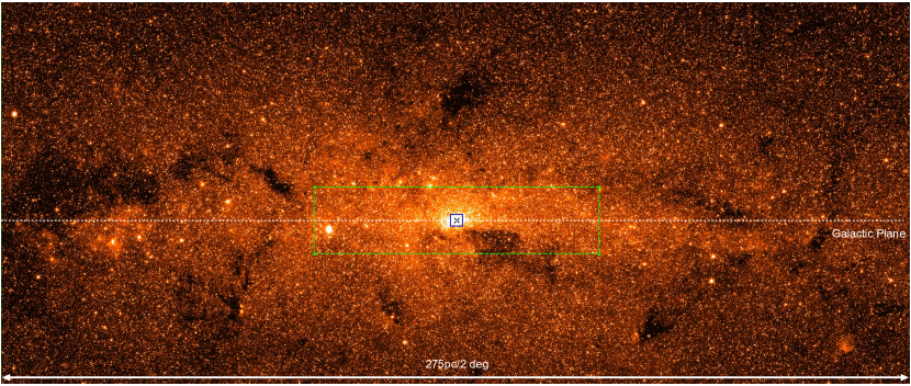
Figure 1: Extinction-corrected $4.5\mu$m Spitzer/ IRAC image of the GC from Schödel et al. (2014a). Galactic north is up and Galactic east is to the left. The blue square outlines the NACO FOV of $\sim$ $1.5^{\prime}\times 1.5^{\prime}$ ($\sim$ $3.6$ pc $\times$ $3.6$ pc) and the green rectangle the HAWK-I FOV of $\sim$ $35.8^{\prime}$ $\times$ $8.4^{\prime}$ ($\sim$ $86$ pc $\times$ $20.2$ pc). Sgr A* is located at the position of the black cross.

2.1 HAWK-I data

We use $Ks$-band data obtained with the near-infrared camera High Acuity Wide field K-band Imager (HAWK-I) at the ESO VLT from the GALACTICNUCLEUS survey, a JHKs imaging survey of the center of the Milky Way (see Nogueras-Lara et al. 2018a, 2019a). We use the central $14$ fields of the survey described in detail in Nogueras-Lara et al. (2019a) that together compose a region of about $84.4$ pc x $21$ pc (see the green rectangle in Fig.  1) around Sgr A*. We do not have field 7 (black rectangle to the northeast in Fig.  2) because the data were obtained under poor observing conditions. Since this field is at a radial distance of more than $11$ pc from Sgr A*, we assume that it is not very significant for studying the NSC (half-light radius $\sim 3-5$ pc).

2.2 NACO data

The data and their reduction are described in detail in Gallego-Cano et al. (2018); they provide an angular resolution of about $0.070^{\prime\prime}$ FWHM over a field of about $1.5^{\prime}x1.5^{\prime}$. In particular, we use $Ks$-band data from 11 May 2011 obtained with the S27 camera ($0.027^{\prime\prime}$ pixel scale) of NACO installed at the ESO VLT. It is the largest field observed by NACO and is therefore the best option for studying the large-scale structure of the NSC. Even though the data are relatively shallow, they are of excellent quality and are well-suited to studying the central parsecs at the GC in the magnitude ranges of stars that we want to analyze ($K_{s}\leq 16$).

3 Stellar number density maps

The steps to create the stellar density maps are the following:

1. Alignment of NACO and HAWK-I data via a two-degree polynomial fit (IDL POLYWARP and POLY_2D procedures). We perform iterative fits using lists of detected stars in the images to compute the parameters.

2. Application of an inner mask to HAWK-I data with the shape of the NACO data FOV in the central $\sim 1.5$ pc.

3. The joining of NACO and HAWK-I data by registering the astrometry of the detected sources in the overlapping region and using NACO in the inner region.

4. Exclusion of all spectroscopically identified early-type stars, that is, massive and young ones, from our sample (using the data of Do et al. 2013).

5. Application of an extinction correction to compute the intrinsic magnitudes for the stars (see section 3.2).

6. Selection of the range of $K_{s}$-magnitude of the stars (see section 3.3).

7. Creation of the maps using 2D density functions (IDL HIST_2D procedure). We assume a bin size of $5^{\prime\prime}\times 5^{\prime\prime}$. (See Appendix A.4 where we study the selection of the bin size).

8. Computation of the mean density in the overlap region between HAWK-I and NACO data.

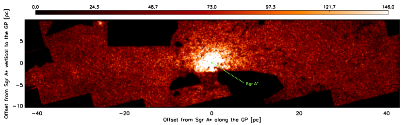
Figure 2: Extinction-corrected stellar number density map of the central $86$ pc $\times$ $20.2$ pc of the Galaxy for stars with $11.0\leq K_{s}\leq 16.0$ ($9.0\leq K_{s,extc}\leq 14.0$). The magnitudes of individual stars were corrected for extinction using the extinction map of Dong et al. (2011). The dark patches in the image correspond to the green polygons in the extinction map (see Fig. 5). Sgr A* is located at the green star. Galactic north is up and Galactic east is to the left. The Galactic plane runs horizontally.

The image in Fig.  2 shows the extinction-corrected density map for stars in the range $9.0\leq K_{s,extc}\leq 14.0$, where $K_{s,extc}$ is the extinction-corrected magnitude.

3.1 Crowding and completeness

For HAWK-I data, we study $14$ fields that have different quality mostly because of the different atmospheric seeing conditions during the observations. We take special care in analyzing the central $10$ parsecs because this is the most crowded region in the whole field and may therefore have a higher incompleteness. Firstly, we create masks to take into account the inhomogeneity of the field, as well as the different crowding in the regions. Figure 2 shows the extinction-corrected density map for stars in the magnitude range of $9.0\leq K_{s,extc}\leq 14.0$ , where we can see regions with different stellar number density. We use the density map in order to create two masks: a global mask, where regions with extremely low (large IR dark clouds to the SW) and high density (H2 regions to the NE, and the Arches and Quintuplet clusters at projected distances of 26–32 pc from the SMBH, respectively) are masked; and a local mask to take into account the different completeness of the fields. For the former, we test four different density thresholds to mask out regions with low density due to high extinction (e.g., the two filaments to the NW). We create four global masks where 30, 40, 50, and 60% of the pixels with low density are excluded (Mask 1 - least restrictive, to Mask 4 - most restrictive). For the latter, we mask positions in the density maps where the values are too low or high by comparing with their neighbors. For each position in the density map, the mean density is computed assuming the values of the density in the closest positions inside a ring with a radius of $15^{\prime\prime}$ ($0.6$ pc), rejecting the points whose values are larger than 1$\sigma$ from the mean. The final masks are obtained by multiplying both local and global masks (see more details in Appendix A.2).

In order to determine the faintest magnitude down to which the counts can be assumed to be complete for all fields, we study the $K_{s}$-luminosity functions (KLFs) of the individual fields after applying Mask 3. Figure  3 shows a comparison between the KLFs determined from our mosaic (the black line) and those from the worst field (the red line), the best field (the blue line), and NACO data (the dashed line). The regions where the KLFs are computed are circular with a radius of $1.5$ pc centered at a distance of $\sim 6$ pc from Sgr A* to the west (the worst field), and a distance of $\sim 29$ pc to the NE (the best field), respectively. The KLF from NACO data is computed in the central $\sim 1.5$ pc around Sgr A*. The faintest magnitude down to which the counts can be assumed complete is $K_{s,extc}=14.0$ ($K_{s}\sim 16.0$) for all fields (the dotted straight line in Fig. 3).

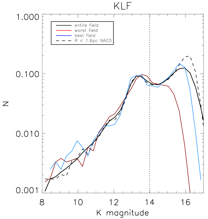
Figure 3: Comparison between the KLFs determined from the entire field (black line) and those from the worst field (red line), the best field ( blue line), and NACO data (dashed line). The KLFs are computed after correcting the magnitude of each star using the extinction map of Dong et al. (2011) and applying Mask 3. The dotted straight line indicates the faintest magnitude down to which the counts can be assumed complete for all fields.

We do not apply a completeness correction for NACO data because the high-angular-resolution data used here are complete in the range of magnitudes that we study ($K_{s}\leq 16.0$, see Gallego-Cano et al. 2018). We do not apply a completeness correction for HAWK-I data either but we apply masking generously to those regions with very low density, as we described above.

We analyze the completeness of HAWK-I in the central $\sim$1.5 pc by comparing with NACO data. We define the completeness of HAWK-I in the central region as the number of stars from HAWK-I data divided by the number of stars from NACO data. Figure  4 shows the completeness maps computed for different magnitude ranges. We can see that in the overlapping region the completeness is greater than 88% for stars brighter than $K_{s,extc}=14.0$. Therefore, we do not apply a factor of overlapping to join the data but take the mean between NACO and HAWK-I data in the overlapping region to ensure a smoothed transition between both data sets.

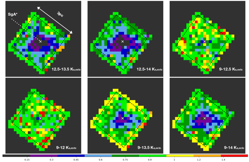
Figure 4: Completeness maps for HAWK-I in the central $\sim 1.5$ pc of the Galaxy by comparing with NACO data. The maps represent the number of stars from HAWK-I data divided by the number of stars from NACO data. The region where only NACO data are used to create the density maps is outlined in the panels by the dashed black square. The outer region is the overlapping region, where we take the mean between both data sets. We can see that the completeness is greater than 88% in the edges in all cases, and therefore we do not apply any scaling factor when we join the data.

3.2 Extinction

We do not correct the effect of extinction on the density of the detected sources because we exclude highly extincted regions. Furthermore, in fields with moderate extinction, differential extinction is $\leq 1$ mag. Since our detection limit is about $K_{s}\sim 18-19$ in all fields, but our completeness cut off (due to data quality and crowding) is $K_{s}=16$, these variations in extinction are not considered to have any significant impact on our results. We correct the magnitudes of the individual stars using the extinction map of Dong et al. (2011). These latter authors created the extinction map using $F187N$ and $F190N$ filters from the Hubble Space Telescope/Near-Infrared Camera and Multi-Object Spectrometer (HST/NICMOS). In order to convert into $K_{s}$ magnitude, we assume that the extinction curve in the NIR can be described by a power law (e.g., Nishiyama et al. 2008; Fritz et al. 2011) and we use the extinction index obtained by Nogueras-Lara et al. (2018a) $\alpha=2.30\pm 0.08$. Figure  5 shows the extinction map of Dong et al. (2011) converted into $K_{s}$ magnitude. We compute the intrinsic $K_{s,extc}$ magnitude for individual stars using the obtained extinction map. Figure 2 shows the extinction-corrected density map for stars with $9.0\leq K_{s,extc}\leq 14.0$. The shape of the FOV of the density map is due to the FOV of the extinction map. Because of dark foreground clouds, the source density in the map of Dong et al. (2011) is very low and the extinction was averaged over large regions. The latter can be easily identified as large patches in the extinction map that hardly show any variation. We mask those regions by hand because they will be heavily contaminated by foreground stars (see green polygons in Fig. 5). The same stars are not necessarily used in the uncorrected density map (without applying extinction correction) and in the extinction-corrected density map because the extinction correction may move stars in and out of the faintest considered bin. In Appendix A.1, we provide further tests to study the systematic uncertainty derived by the extinction-correction, such as considering a less steep value for the extinction index $\alpha$.

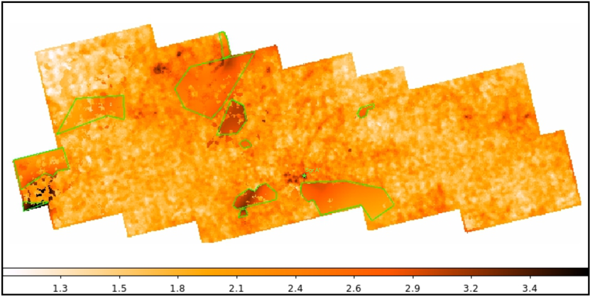
Figure 5: Extinction map $A_{K_{s}}$ from the central $416$ arcmin² ($\sim$1 kpc²) used for the extinction correction. The extinction map is computed by converting the extinction map of Dong et al. (2011) into $K_{s}$ magnitude. We apply masks to some regions (green polygons). The median value of $A_{K_{s}}$ is $1.9$. The spatial resolution is $\sim 9.2$ arcsec. The green star shows the position of Sgr A*.

3.3 Selection of the magnitude ranges for the analyzed stars

In order to test whether the composition of the stellar population in the MWNSC changes with distance from Sgr A*, we study the density maps in the following brightness ranges (in parentheses for extinction-corrected magnitudes):

1. RC stars and bright giants in the ranges: $11.0\leq K_{s}\leq 16.0$ ($9.0\leq K_{s,extc}\leq 14.0$);

2. only bright giants in the ranges: $11.0\leq K_{s}\leq 14.0$ ($9.0\leq K_{s,extc}\leq 12.0$);

3. RC stars in the ranges: $14.5\leq K_{s}\leq 16.0$ ($12.5\leq K_{s,extc}\leq 14.0$).

We selected the magnitude ranges of RC and bright stars so as to avoid mixing different kinds of stars. The magnitude ranges in the uncorrected density maps are selected in order to consider roughly the same number of stars as in the extinction-corrected density maps. We study the brightness ranges (a) in order to compare with previous studies. Although we do not need any precision photometry, we select the brightest magnitude in the range of the stars in order to avoid saturation effects in our sample. Furthermore, in Appendix A.8 we explore the results by considering another brightest magnitude limit.

4 Structure of the nuclear stellar cluster

Our main goal is to study the structure of the MWNSC. Since the MWNSC is not isolated, when we compute the star density toward the GC we have to take into account several superposed components: NSD, GB, and GD (in decreasing order of star density). The GD contributes a negligible contamination within the central $\sim 10$ pc (see the possible contamination by stars in the GD in Appendix A.6). The primary source of systematic uncertainty is due to the NSD, and the secondary one is due to the GB. We apply the term ”background” to both foreground and background contributions that contaminate our sample. We use the stellar density map of the central $6^{\circ}\times 2^{\circ}$ of our Galaxy from Nishiyama et al. (2013) to model the GB and NSD in order to subtract them from the data and isolate the NSC in the stellar density maps (see left panel in Fig. 7). Finally, we fit Sérsic functions to the stellar density maps of the MWNSC. Furthermore, we use MIR Spitzer images to constrain the shape of NSC and NSD, following up the work of Schödel et al. (2014a).

4.1 Galactic bulge

We model the GB as a triaxial ellipsoidal bar with a centrally peaked volume emissivity $\rho$ (Dwek et al. 1995; Stanek et al. 1997; Freudenreich 1998). We assume the best GB parameters computed by Launhardt et al. (2002, see Table 4 in their paper and Table 1 in the present paper). These latter authors found that the best fit for the surface brightness profile of the GB is the one that represents the volume emissivity by an exponential model:

$$\rho(r)\propto exp(-R_{s}).$$ (1)

They selected the shape of the bar as a ”generalized ellipsoid” (Athanassoula et al. 1990; Freudenreich 1998), where $R_{s}$ is the effective radius (see equations 5 and 6 in Launhardt et al. 2002).

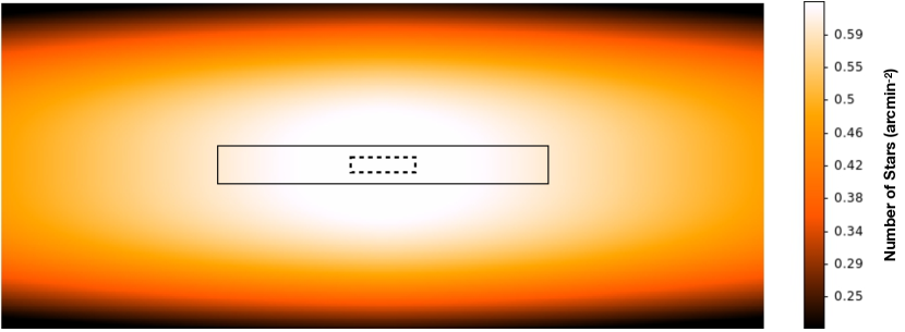
Figure 6: Triaxial ellipsoidal bar model with a centrally peaked volume emissivity $\rho$ for the GB of the central $6^{\circ}\times 2^{\circ}$ ($\sim$ 864 pc $\times$ 288 pc) of our Galaxy. The inner black dotted rectangle indicates the FOV of our data ($\sim$ 86 pc $\times$ 20.2 pc) and the outer black rectangle indicates the region occupied by the NSD ($\sim$ 460 pc $\times$ 40 pc). Sgr A* is located in the middle of the image. Galactic north is up and Galactic east is to the left. The GP runs horizontally through the center.

The intensity of light from the bulge region in the $\{l,b\}$ direction is given by an integral of the volume emissivity $\rho$ along the line of sight $s$ (for more details see equation  1 of Dwek et al. 1995):

$$I(l,b)=2\cdot N_{0}\cdot\int_{0}^{\infty}exp(-R_{s})\cdot ds.$$ (2)

We apply the previous equation to compute the projected stellar number density of the GB. The parameter $N_{0}$ is a normalization constant given in units of stellar number density and is determined by fitting the model $I(l,b)$ to the stellar number density map from Nishiyama et al. (2013). We mask a region of $\sim 500$ $\times$ $72$ pc² centered on Sgr A* occupied by the NSD (Launhardt et al. 2002) and some dark clouds to fit the GB. We assume that its central stellar density can be derived from its outer parts. Figure  7 shows the GB model that fits for the stellar density map. Table 1 summarizes the parameters that we assume in the model and the value of $N_{0}$ that we obtain.

4.2 Nuclear stellar disk

In this section, we analyze the NSD, the component with the overall highest star density and smallest angular scale. We model the NSD using the stellar density map of the central $6^{\circ}\times 2^{\circ}$ of our Galaxy of Nishiyama et al. (2013). We mask regions with low density (see dark clouds in the right-hand image in Fig.  7) and a region of approximately $10$ pc $\times$ $10$ pc centered on Sgr A* occupied by the NSC. The NSD can be modeled by an elliptical model. We use a Sérsic model (Graham 2001) given by

$$I(x,y)=I_{e}exp\bigg{\{}-b_{n}\bigg{[}\bigg{(}\frac{p}{R_{e}}\bigg{)}^{1/n}-1\bigg{]}\bigg{\}},$$ (3)

where $I_{e}$ is the intensity at the effective radius $R_{e}$, which encloses $50\%$ of the light. The factor $b_{n}$ is a function of the Sérsic index $n$. We use the approximation $b_{n}=1.9992n-0.32$ given by Capaccioli (1987) for $1<n<10$. We use the modified projected radius $p$ for elliptical models

$$p=\sqrt{x^{2}+(y/q)^{2}},$$ (4)

where $x$ and $y$ are the 2D coordinates and $q$ is the ratio between minor and major axis. We are interested in studying the star count contribution of the NSD, and therefore we convert the $I(x,y)$ into stellar number density in the $\{x,y\}$ position. Finally, we fit the Sérsic model for the NSD after subtracting the GB model computed in the previous section to the stellar number density map. The best-fit parameters were obtained using a gradient-expansion algorithm to compute a nonlinear least squares fit to the model (IDL CURVEFIT procedure). The value of $\chi^{2}_{reduced}$ is $1.082$. The best-fit parameters are summarized in Table 1.

Table 1: Galactic bulge and nuclear stellar disk Model 1 parameters using the stellar density map of the central $6^{\circ}\times 2^{\circ}$ of our Galaxy of Nishiyama et al. (2013).

Galactic bulge
Parameters	Value
Sun dist. from GC $R_{0}^{\mathrm{a}}$	8.5 kpc
Bar X scale length $a_{x}^{\mathrm{a}}$	1.1 kpc
Bar Y scale length $a_{y}^{\mathrm{a}}$	0.36 kpc
Bar Z scale length $a_{z}^{\mathrm{a}}$	0.22 kpc
Bar face-on parameter $C_{\bot}^{\mathrm{a}}$	1.6
Bar edge-on parameter $C_{\parallel}^{\mathrm{a}}$	3.2
Normalization constant $N_{0}$	($9.90\pm 0.02$) stars/arcmin2
Nuclear stellar disk
Parameters	Value
Stellar number density at $R_{e}$	($19.84\pm 0.16$) stars/arcmin2
Flattening $q$	($0.338\pm 0.002$)
Sérsic index $n$	($0.782\pm 0.008$)
Effective radius $R_{e}$	($116.2\pm 0.6$)pc

• Fixed input parameter from Launhardt et al. (2002).

Although we assume a larger value for the distance of the GC to compute the GB, if we assume a more updated value of 8 kpc (see, e.g., Genzel et al. 2010; Meyer et al. 2012; Gravity Collaboration et al. 2018) the differences between the parameters obtained using both values are negligible ($<0.001\%$).

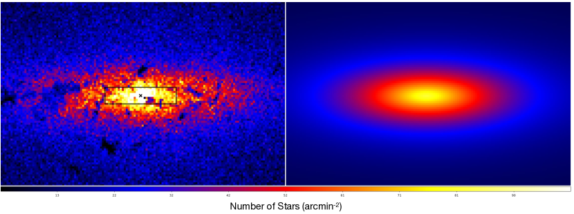
Figure 7: Map of the stellar density in the central 341 pc $\times$ 219 pc of our Galaxy. Both panels use the same color linear scales. Left panel: Stellar number density map from Nishiyama et al. (2013). The black rectangle indicates the FOV of our data ($\sim$ $86$ pc $\times$ $20.2$ pc). Sgr A* is located in the position of the black cross. Right panel: Sérsic plus triaxial ellipsoidal fit to the data after masking the central 10 pc occupied by the NSC and regions with low density.

4.3 Sérsic models

4.3.1 NSC aligned with respect the GP

The Sérsic model gives a good description of the large-scale structure of the NSC (Schödel et al. 2014a). We apply it to the extinction-corrected density maps computed for the different magnitude ranges of the stars (see section 3.3) and use the following steps to fit the models:

1. We apply a mask to take into account the variable completeness across the FOV due to the different observing conditions, extinction, and crowding, as we saw in section 3.1. We study the systematic errors caused by the selection of the masks in Appendix A.2.

2. To avoid biased results in the Sérsic model, which has a central peak, we mask the inner $0.6$ pc. This is due to the fact that in our study, the number counts are dominated by bright stars with $K_{s}<16.0$ that show a flat profile, different from the cusp profile, which is shown by faint stars with $K_{s}>16.0$ (see Buchholz et al. 2009; Bartko et al. 2010; Yusef-Zadeh et al. 2012; Do et al. 2013; Gallego-Cano et al. 2018; Schödel et al. 2018).

3. We fit a Sérsic NSC fit to the stellar density maps for the different magnitude ranges, including the models computed for the GB and the NSD in Sects 4.1 and  4.2, respectively. Only the stellar number density at effective radius for the NSD is scaled to the maps, keeping the ratio GB/NSD constant.

4. We fix the tilt angle between the NSC with respect to the GP to $0$ degrees. In the following section, we leave this angle free.

We found the best-fit solution by using a gradient-expansion algorithm to compute a nonlinear least squares fit to the model with five or six parameters (IDL MPCURVEFIT procedure), depending on whether the inclination angle between NSC and GP is fixed or free, respectively (see the following section). We explored the systematic effects of the different choices of masks and other parameters by changing their values and fitting the data repeatedly. The resulting best-fit values are listed in Table 8. Figure 8 shows the comparison between the density map for stars with $9.0\leq K_{s,extc}\leq 14.0$ (upper panel) and the Sérsic model plus the background model (middle panel) that we obtain in the fit (ID 10 in Table 8). The lower panel shows the residual image given by the difference between the density map and the model divided by the uncertainty map of the density map. The uncertainty map is created by taking the square root of the values in the stellar density map. The residual map is not completely homogeneous, but the differences along the FOV are $<2.5\sigma$ and are concentrated in the inner 1-2 pc, which is probably related to the fact that we have mixed different data sets. These differences are smoothed and the averages of the residuals are smaller when the tilt angle between the NSC and the GP is free in the fits, as we can see in Fig. 10.

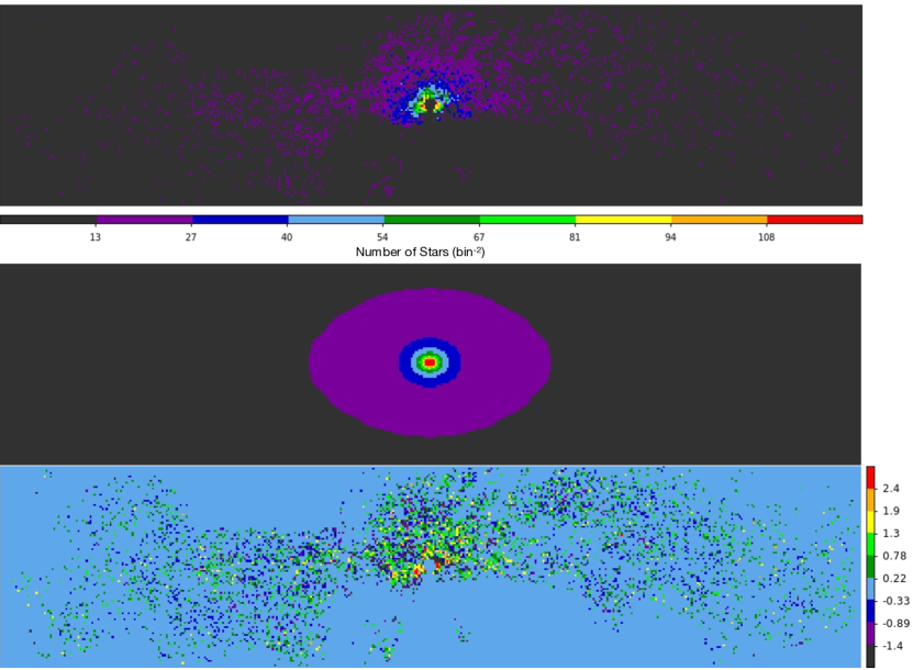
Figure 8: Comparison between the stellar density map of the central $86$ pc $\times$ $20.2$ pc of the Galaxy and the model. Upper: Extinction-corrected stellar density map for stars with $9.0\leq K_{s,extc}\leq 14.0$. The dark regions are masked in the fit. Middle: Sérsic model for the NSC plus the background model (ID 10 in Table 8). Lower: Residual image given by the difference between the upper and middle panels divided by the uncertainty map of the density map. The color bar shown for the lower panel is in units of the standard deviation. The other two panels use the same linear color scale. Galactic north is up and Galactic east is to the left.

As a second approach to the problem, we symmetrize the cluster with respect to the GP and with respect to the Galactic north–south axis through Sgr A*. We obtain the symmetrized image by replacing each pixel in each quadrant with the median of the corresponding pixels in the four image quadrants and ignoring the masked areas. The pixels along the vertical and horizontal symmetry axes are not averaged. The uncertainty for each pixel is computed by taking the standard error of the mean. Figure 9 shows the comparison between the stellar density map (upper panel) and the symmetrized image (middle panel) for stars with $9.0\leq K_{s,extc}\leq 12.0$ (ID 7 for Table 8). We fit the Sérsic model to the symmetrized images corresponding to the different magnitude ranges.

The resulting best-fit values are listed in Table 8. Table 2 shows the final parameters that we obtain taking the mean value of the best-fit parameters from Table 8. The uncertainties are the standard deviations of all the best-fit parameters. We add the statistical errors quadratically to the final uncertainties.

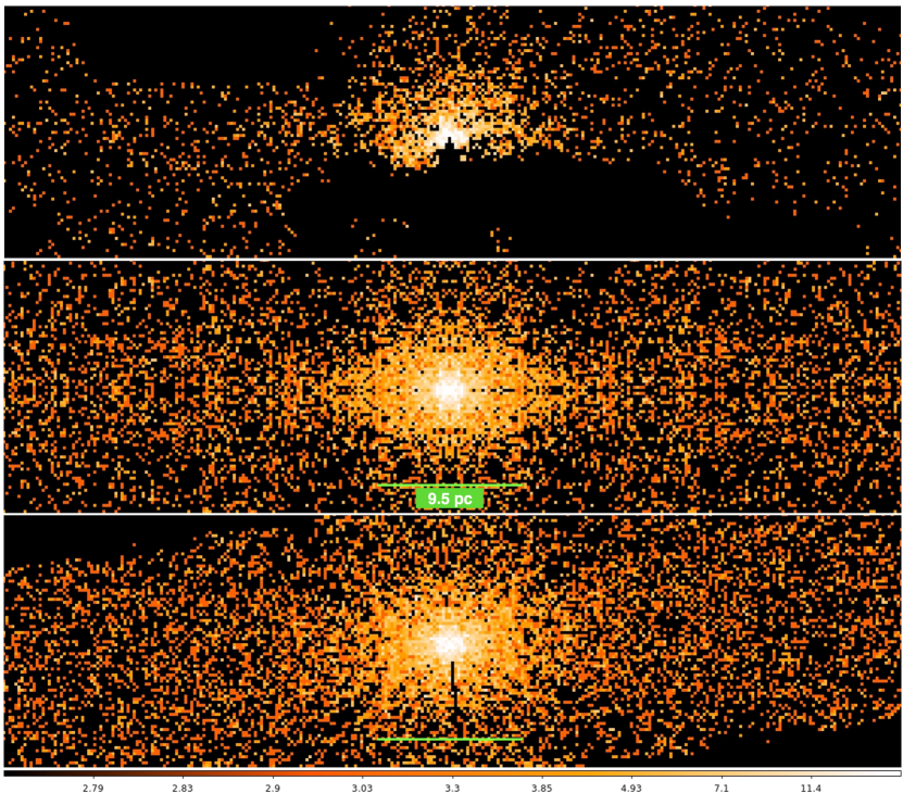
Figure 9: Comparison between the stellar density map of the central $58$ pc $\times$ $16$ pc of the Galaxy and the symmetrized images. Upper: Extinction-corrected density map for stars with $9.0\leq K_{s,extc}\leq 12$. The mask applied is shown (dark regions). Middle: Symmetrized image is obtained from taking the median of the pixels from the four quadrants by assuming symmetry of the cluster with respect to the GP and with respect to the Galactic north–south axis through Sgr A*. Lower: Symmetrized image obtained by assuming symmetry of the cluster with respect to tilted axes through Sgr A* with an angle of $\sim-5.6$ degrees. The three panels use the same color scale. Galactic north is up and Galactic east is to the left.

Table 2: Best-fit model parameters for Sérsic fits to the stellar number density maps. The MWNSC is aligned with respect to GP.

ID	Mag. range	$N^{b}_{e,nsd}$	$N^{c}_{e,nsc}$	$q^{d}$	$n^{e}$	$R^{f}_{e}$
	($K_{s,extc}$)	(stars/bin2,a)	(stars/bin2,a)			(pc)
1	$12.5-14$	$2.45\pm 0.10$	$3.94\pm 0.68$	$0.85\pm 0.05$	$2.59\pm 0.27$	$5.66\pm 0.32$
2	$9-12$	$0.55\pm 0.09$	$1.16\pm 0.26$	$0.60\pm 0.04$	$2.28\pm 0.47$	$4.57\pm 0.78$
3	$9-14$	$3.22\pm 0.19$	$6.55\pm 1.08$	$0.78\pm 0.02$	$2.02\pm 0.46$	$5.38\pm 0.21$

4.3.2 Tilt angle

In this section, we explore the effect of leaving the tilt angle between the NSC and the GP free in the fits without assuming any symmetry of the cluster a priori. First of all, we create different symmetrized maps varying the tilt angle $\theta$ from $\theta=0^{\circ}$ (NSC aligned to the GP) to $\theta=-15^{\circ}$ (NSC is symmetric with respect to an axis rotated $\theta$ with respect to the GP and with respect to an axis perpendicular to GP through Sg A*). We compute the residual images given by the difference between the stellar density map and the symmetrized image. Figure 10 shows the average of the residual maps given by the root mean square of all values for the different magnitude ranges. We can see that there is an improvement in the residual for a tilted symmetrized cluster compared to a nontilted one. For bright stars, we find a minimum value around $\theta=-6^{\circ}$ (middle panel in Fig. 10). For RC stars, we find a minimum around $\theta=-5^{\circ}$ (left panel in the figure). We obtain similar results for stars with $9.0\leq K_{s,ext}\leq 14.0$ (right panel in the figure). For all cases, the average of the residuals are very similar from $\theta=0^{\circ}$ to $\theta=-10^{\circ}$. We also performed a fit of NSC + NSD on the untilted and unsymmetrized map, this time introducing the tilt angle as an additional free parameter. As we can see in Fig. 10, there are local minima for the value of $\theta$, which encouraged us to explore the fits considering different initial values for the angle (see Appendix A.10).

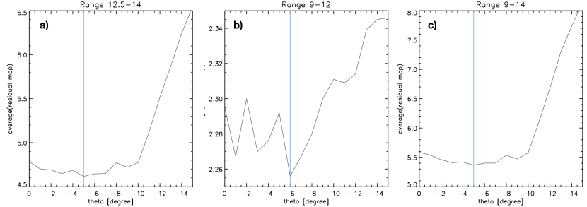
Figure 10: Average of the residuals in the difference image between the original and the symmetrized image of the NSC vs. the value of the tilt angle $\theta$ used to symmetrize the image. a) Average of the residuals for stars with $12.5<K_{s,ext}<14.0$. We find a minimum at $\theta=-5^{\circ}$ that is not very significant. b) Average of the residuals for stars with $9.0<K_{s,ext}<12.0$. We find a minimum for $\theta=-6^{\circ}$. c) Average of the residuals for stars with $9.0<K_{s,ext}<14.0$. In this case, we obtain similar results for stars with $12.5<K_{s,ext}<14.0$. For the three cases, the residuals are similar from $\theta=0^{\circ}$ to $\theta=-10^{\circ}$. The blue lines indicate the value of $\theta$ that minimizes the residuals.

The resulting best-fit values are listed in Table 9. The lower panel of figure 9 shows the symmetrized image corresponding to ID 7 in Table 9. Table 3 shows the final results that we obtain taking the mean value of the best-fit parameters from Table 9 and the uncertainties are the standard deviations of the systematic errors. The statistical errors for the parameters are negligible. In the case of $\theta$, we have to also include the systematic errors associated to the selection of different initial $\theta$ (see Appendix A.10). In this case, we also assume the statistical errors. The value of $\theta$ obtained for bright stars is very consistent with the value that minimizes the residuals. For the other stars, the values are inside the range of the angles that minimize the residuals.

Table 3: Best-fit model parameters for Sérsic fits to the stellar number density maps. The tilt angle between the NSC and the GP is a free parameter in the fits.

ID	Mag. range	$\theta^{a}$	$N_{nsd}$	$N_{nsc}$	$q$	$n$	$R_{e}$
	($K_{s,extc}$)	(degree)	(stars/bin2)	(stars/bin2)			(pc)
1	$12.5-14$	$-8.51\pm 3.15_{sys}\pm 0.66_{stat}$	$2.43\pm 0.10$	$3.38\pm 0.61$	$0.83\pm 0.04$	$3.01\pm 0.39$	$6.19\pm 0.68$
2	$9-12$	$-5.60\pm 1.28_{sys}\pm 0.57_{stat}$	$0.55\pm 0.08$	$1.24\pm 0.25$	$0.64\pm 0.10$	$1.93\pm 0.50$	$4.31\pm 0.52$
3	$9-14$	$-6.98\pm 1.25_{sys}\pm 0.40_{stat}$	$3.21\pm 0.20$	$6.63\pm 1.27$	$0.75\pm 0.01$	$2.26\pm 0.21$	$5.36\pm 0.36$

4.4 Best-fit NSC parameters from MIR imaging

To obtain an independent constraint on the projected structure of the NSD plus NSC, we also fit our models to IRAC/Spitzer $4.5\mu$m images (see Fig. 1). We use the same data and technique as outlined in Schödel et al. (2014a). However, while the latter authors used images no larger than $200$ pc $\times$ $200$ pc in order to avoid the difficulties of the spatial change in the background contributed by the GB and due to large dark clouds, here we fit the NSD to the full images ($\sim$ $300$ pc $\times$ $250$ pc) as delivered by the survey of Stolovy et al. (2006) and include our GB model to take the influence of the latter into account. All large dark clouds were masked. By using the full extent of the images from the Spitzer survey we expect to obtain better constraints on the NSD with its large scale length. We repeat the double Sérsic NSC plus NSD fit of Schödel et al. (2014a), including also our GB emission model based on Launhardt et al. (2002) and leaving the tilt angle free. Tables 4 and 5 show the final results obtained for the NSD (NSD Model 2) and NSC, respectively. Our results are very similar to what was obtained by Schödel et al. (2014a), but should be better constrained because of the larger FOV and the use of a more accurate GB model. Due to the low resolution of the data, we can only approximately compare the results with the values obtained for stars with $9.0\leq K_{s,extc}\leq 12.0$ (ID 2 in Table 3). All the parameters that we obtain in the fits are consistent with the final results at the $1\sigma$ level.

Table 4: Nuclear stellar disk Model 2 using MIR imaging.

Nuclear stellar disk
Parameter	Value
$I_{e}^{\mathrm{a}}$	($0.279\pm 0.003$) mJy arcsec-2
$q$	($0.372\pm 0.005$)
$n$	($1.09\pm 0.03$)
$R_{e}$	($86.9\pm 0.6$)pc

• Flux density at $R_{e}$.

Table 5: Nuclear stellar cluster model parameters using MIR imaging.

Nuclear stellar cluster
Parameter	Value
$\theta^{\mathrm{b}}$	$(-6.9\pm 1.7)$ degree
$I_{e}^{\mathrm{a}}$	($2.64\pm 0.43$) mJy arcsec-2
$q$	($0.66\pm 0.03$)
$n$	($1.8\pm 0.1$)
$R_{e}$	($4.9\pm 0.5$)pc

• Flux density at $R_{e}$.

• Tilt angle defined positive in the direction east of Galactic north.

5 Discussion

5.1 Overall properties of the MWNSC

The present paper fills some of the gaps that may be present in previous studies. We address the study of the MWNSC properties using two independent methods: an improved analysis of IRAC/Spitzer MIR images, which are less affected by interstellar extinction than NIR images (Nishiyama et al. 2009; Fritz et al. 2011), and analyzing star counts and higher-resolution NIR images of NACO and HAWK-I. We aim to build a bridge between the last two comparable studies of Schödel et al. (2014a) and Fritz et al. (2016) and improve on their shortcomings, as described in the following.

Table 6 shows a comparison between the results obtained here and in previous studies. The values inferred in this and in previous studies agree within their $1-2\sigma$ uncertainties, indicating that none of them suffer any major bias. Due to the higher angular resolution achieved in our study, we are able to constrain the range of the stars to investigate the distribution of giants in the RC and at brighter magnitudes, separately. Due to its generally very well defined brightness and mass, the RC is a very well suited tracer to studying stellar structures older than $\sim 2$ Gyr. The RC stars are the most abundant stars at $K_{s}\leq 17$ in the GC and are therefore an important tracer population, but these were not isolated in previous studies because of their low angular resolution, which meant that brighter stars dominated the measurements.

We use the same NIR wavelength and method of star counts as Fritz et al. (2016) but with a more than twice higher angular resolution, which allows us to use the RC as a tracer of structure, limit the influence of crowding, and improve the number statistics. Also, we explicitly model and take into account stellar structures that overlap with the NSC along the line of sight, in particular the Galactic bulge and the nuclear stellar cluster. Finally, Fritz et al. (2016) could not clean their sample of foreground stars across their entire field because they did not have two filter measurements for all regions. Here, we can reliably exclude foreground stars.

Schödel et al. (2014a) use MIR images and study also the contribution of the GB and NSD. The disadvantages are that the resolution is lower than in our study and they only used the central most parts of the images available to them, which may have biased their work. We repeat their study and improve on it by analyzing the images in their entirety and including the GB model.

In order to give the final values of the MWNSC parameters, ID 1 and ID 2 in Table 3 can be taken as independent measurements because the samples that we study in each case are different; they are composed of stars in two different ranges of magnitude. If we add also the results from MIR imaging (Table 5), we can assume that the final values obtained from our work are the mean of the three parameters and the uncertainties are the standard deviations of them. We obtain an effective radius: $R_{e}=(5.1\pm 1.0)$ pc; an axis ratio: $q=0.71\pm 0.10$; a tilt angle: $\theta=(-7.0\pm 1.5)$ degrees ; and a Sérsic index: $n=2.2\pm 0.7$. The ellipticity is $\epsilon=1-q=0.29\pm 0.10$. The effective radius and the ellipticity of the MWNSC are very well constrained (see Fig. 11). Fritz et al. (2016) study the flattening in different ranges of distance from the SMBH. These latter authors report $q=0.80$ at distances smaller than $2.3$ pc, but for larger distances, they obtain larger values of the flattening, very similar to our results. The reason for these somewhat different results is probably linked to the fact that they do not take into account the MWNSC as a separate entity from the GB and NB. The value of the Sérsic index is highly dependent on the distribution in the central parsec. Fritz et al. (2016) consider the central parsec in the fits in the same way that we do in the present work, but we mask the central $0.6$ pc to avoid contamination from young stars and biases results of the fits because of the flat profile showed by bright stars (Gallego-Cano et al. 2018). Schödel et al. (2014a) reported a smaller value for the Sérsic index than ours. The difference comes from the NIR images, because they are forced to mask the central parsec because of the low resolution of the data and the existence of a few extremely bright sources and a strong diffuse emission from the mini spiral. It appears that the Sérsic index is very susceptible to bias and caution is required in its application. Its precise value also depends strongly on the assumptions on, and fit of, any structures overlapping with the NSC.

Both of these latter two studies quote that they may underestimate the systematic errors in component fitting. We give very robust and reliable uncertainties on the best-fit NSC parameters, not only by taking into account different potential sources of systematic error but also by analyzing the MWNSC structure using two completely different approaches: MIR and NIR imaging. We explore in detail the systematic uncertainties that can affect the parameters, taking into account different potential sources of systematic error. We choose to let these uncertainties be reflected in the error bars of the best-fit parameters in order to give robust and reliable values.

Finally, in addition to assuming that the MWNSC is aligned with respect to the GP, as in previous studies (upper panels in Fig. 12), we leave the tilt angle between the NSC and the GP to be free in the Sérsic models (lower panels in Fig. 12). We obtain novel photometric data that suggest that the MWNSC is consistent with a tilt of the major axis out of the Galactic plane by up to -10 degrees. This result corroborates the misalignment of the kinematic position angle of $\sim-9$ degrees found by Feldmeier et al. (2014), which is somewhat smaller but is within the uncertainties. Fritz et al. (2016) also determine the orientation of the major axis in proper motion data, finding that it agrees within 1.2 degrees with the GP, in contrast to line of sight and star distribution data. This latter result suggests that a simple rotation of the cluster is not sufficient to explain all the data. Figure 12 shows a comparison between the symmetrized images of the inner $\sim 42$ pc x $16$ pc of the Galaxy for stars with $12.5\leq K_{s,extc}\leq 14.0$ (left panels) and the Sérsic models (right panels). For upper panels we assume that the MWNSC is aligned with respect to the GP in the fits (ID 3 in Table 8). For lower panels, we leave the tilt angle free in the fits (ID 3 in Table 9).

Table 6: Comparison with previous studies.

Study	Wavelength	Angular resolution	Scales	$q$	$n$	$R_{e}$
	($\mu m$)	(arcsec)	(pc2)			(pc)
Schödel et al. (2014)	$4.5$	$2$	$200\times 200$	$0.71\pm 0.02$	$2\pm 0.2$	$4.2\pm 0.4$
Fritz et al. (2016)	$2.2$	$1$	$80\times 80$	$0.80\pm 0.04$	$1.5\pm 0.1$	$7\pm 2$
Present work NIR	$2.2$	$0.2$	$86\times 20.2$	$0.75\pm 0.01$	$2.26\pm 0.21$	$5.36\pm 0.35$
Present work MIR	$4.5$	$2$	$300\times 250$	$0.66\pm 0.03$	$1.8\pm 0.1$	$4.9\pm 0.5$

Figure 11 shows a comparison between the best-fit parameters for the case when the MWNSC is aligned with the GP and for the case when the tilt angle is left free. The values are consistent with each other inside the uncertainties. Considering also Fig. 10, which shows the average of the residuals obtained by the subtraction of the symmetrized image of the MWNSC from the original image, we can see that it is very difficult to constrain the tilt angle of the system, but out-of-plane tilt of up to $-10^{\circ}$ cannot be excluded.

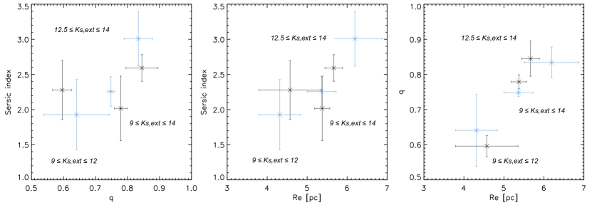
Figure 11: Comparison between the best-fit NSC parameters for a MWNSC that is assumed to be aligned with the GP (black points) or for the case when a small tip-angle is included in the fits (blue points). The magnitude of the stars is indicated in the panels.

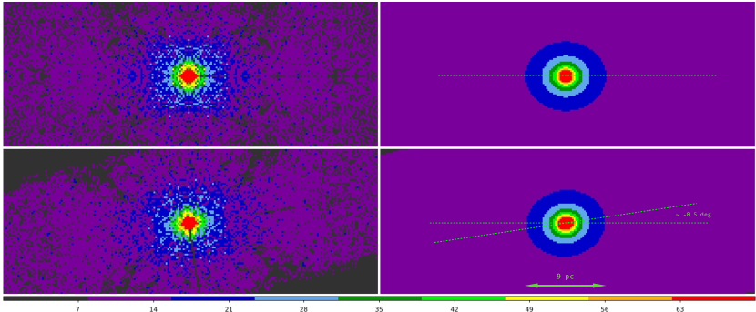
Figure 12: Zoom-in to compare the symmetrized images of the inner $\sim 42$ pc x $16$ pc of the Galaxy for stars with $12.5\leq K_{s,extc}\leq 14.0$ obtained by keeping the angle between the NSC and GP equal to zero (upper panels, ID 3 in Table 8) and leaving the tilt angle free in the fits (lower panels, ID 3 in Table 9). Right panels show the Sérsic model that we obtain from the fits for each case. The color scale is linear and all the images have been scaled identically. Galactic north is up and Galactic east is to the left.

5.2 Distribution of the stars at the Galactic center

The stars in our sample are predominantly giants, mostly in the RC and Asymptotic Giant Branch (AGB) with ages of more than 5 Gyr (Blum et al. 1996; Pfuhl et al. 2011). An overabundance of bright stars has been found in the Nuclear Bulge (NB) formed by the NSD + the MWNSC compared with the stellar population of the GB/Bar (Blum et al. 1996; Philipp et al. 1999). This result is a consequence of different star formation histories of both entities since the GB has not experienced any significant amount of recent star formation, contrary to the NB (see Nogueras-Lara et al. 2018b). The low angular resolution of previous studies made any potential differences between the distribution of RC stars and brighter stars difficult to study. If the ratio between stellar populations of different ages changes, the ratio between the number of bright giants and giants in the RC will change. For example, adding populations of ages $\lesssim 1.5$ Gyr can enhance the number of bright giants in the luminosity function.

In this work we find slightly different best-fit parameters for the MWNSC, depending on whether we fit our models to the star counts of RC stars or those of brighter giants. The $R_{e}$ for RC stars appears somewhat larger than for bright stars, and the distribution of the latter is more flattened. Furthermore, we study the projected radius profiles for both distributions (see Fig. 13). Although the differences between both distributions are not very significant, they may suggest that the distributions of the stellar populations within the MWNSC are not homogeneous, as a result of distinct star formation histories at different distances from the SMBH. The flat distribution of the bright stars may indicate that some of the stars belong to a star formation event or a dissolved star cluster of a few hundred million years old. However, we are unable to make any firm conclusions because the innermost fields of HAWK-I data that correspond to the MWNSC have a lower S/N and are of lower resolution than further out, and greater resolution is required across the FOV to avoid being dominated by systematic error.

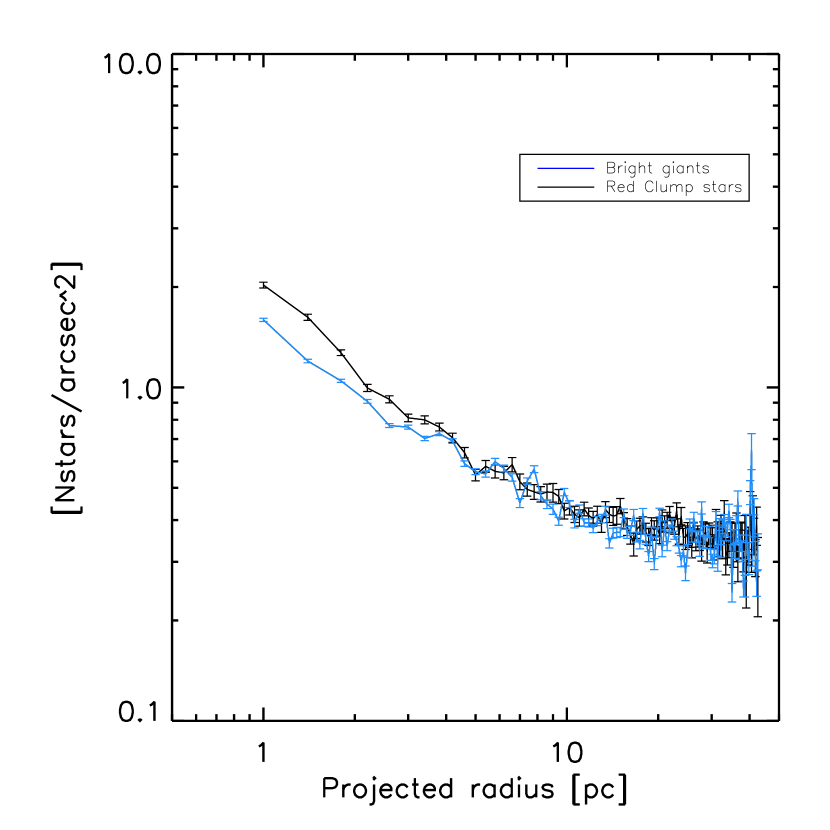
Figure 13: Comparison between the projected radius profiles computed for different ranges of magnitudes along the GP. Only the data closer than 50” (2pc) to the GP are taken into account. The black line shows the density profile for RC stars ($12.5\leq K_{s,extc}\leq 14$) and the blue line indicates the density profile for bright stars ($9.0\leq K_{s,extc}\leq 12$). In order to facilitate the comparison between both profiles, the data for the bright stars are scaled using the median ratio of both number counts at distances larger than $10$pc. We mask the inner 0.6 pc around Sgr A*.

When we fit the Sérsic model to the MWNSC, we subtract the NSD model from it. There are two important caveats. On the one hand, we use the density map from Nishiyama et al. (2013) to model the NSD for NIR images. These latter authors built the density map for stars significantly brighter than those that we analyzed (stars with $K_{s,extc}$ brighter than $8.0$ for the central $20^{\prime}$ and $K_{s,extc}$ brighter than $10.5$ beyond $20^{\prime}$). Unfortunately, we cannot estimate the effect of this difference on our results. However, the fact that we obtain similar results using NIR and MIR data where we use two different NSD models gives us confidence in our results. On the other hand, if the stellar populations are different in the NSC and the NSD, this would also lead to different results for the stars corresponding to different magnitude ranges. Currently, the dissimilarity in the stellar populations has not yet been investigated, but there are indications of differences (Nogueras-Lara et al. 2019b). In conclusion, the hypothesis of different star formation histories depending on the distance from Sgr A* will need to be investigated in a future study using higher angular resolution imaging and spectroscopy.

5.3 New constraints on the structure of the NSD

We present two new analyses of the NSD using completely different data and methods. For one of these, we use the stellar number density map from Nishiyama et al. (2013) of the central $\sim 860$ pc $\times$ $280$ pc of our Galaxy (NSD Model 1, Table 1) with a bin size of $1^{\prime}$, and for the other we derive a density map using IRAC/Spitzer $4.5\mu$m images of the central $300$ pc $\times$ $250$ pc (NSD Model 2, Table 4), with a bin size of $5^{\prime\prime}-7^{\prime\prime}$. The main advantage of using NSD Model 1 is that we apply a similar procedure to fit the Sérsic model to the extinction-corrected stellar number density maps built from NIR images using a star count analysis. Furthermore, the images are larger which allows us to better constrain the GB model. The main advantage of NSD Model 2 is that the images are of higher resolution than the images from NSD Model 1. Also, the MIR images are less affected by extinction and were corrected for it. Taking into account the effect of extinction is of great importance in the highly extincted GC region. In particular, dust in the central molecular zone appears in projection concentrated toward a strip between $\pm 30$ pc around the GP (e.g., Fig. 6 in Schödel et al. 2014a; see also Molinari et al. 2011). Although the brightness of the individual stars in the data set that underlies Model 1 has been corrected for extinction, the overall systematic effect of the nonrandom distribution of highly extinguished regions on this model has not been taken into account. Such a bias would result in a systematically thicker NSD model. Similarly, a gradient of extinction along Galactic longitude can bias the model toward a larger effective radius. We therefore believe that Model 2 is the most accurate one.

5.4 Comparison with extragalactic NSCs

This study is complementary to previous investigations of the structure of the MWNSC. Having addressed the potential shortcomings of previous studies through the use of sensitive, high-angular-resolution star counts over a large field and careful modeling of the surrounding structures, we have now firmly established that the MWNSC has an effective radius of $R_{e}=5.1\pm 1.0$ pc and that it is flattened, with its major axis almost parallel to the Galactic plane. The present study contributes the following two new findings: (1) The major axis of the MWNSC may be tilted out of the Galactic plane by as much as -10 degrees. (2) We find that the giants brighter than the RC show a different distribution to that of the faint stars; in particular, the former display a significantly stronger flattening.

The size and mass of the MWNSC lie well within the distribution of these quantities for other NSCs in spiral galaxies (e.g., Georgiev & Böker 2014; Schödel et al. 2014b). Also, the complex star formation history of the MWNSC is consistent with those of other NSCs. A range of structural variability has also been found in NSCs in other spiral galaxies (Georgiev & Böker 2014). Flattening along the galactic plane and potentially small tilt angles between the NSC major axes and the host galaxy planes have been observed in detail in high-angular-resolution observations of a small number of nearby spirals (Seth et al. 2006; Carson et al. 2015). Figure 14 represents the axis ratio versus tilt angle between the NSC major axis and the galaxy plane for different NSCs in edge-on spiral galaxies (data are from Table 2 in Seth et al. 2006). We average the results from the two different filters for every NSC. Three of the clusters in the sample of Seth et al. (2006, IRAS 09312-3248, NGC 3501, and NGC 4183) are very compact and are surrounded by complex emission; we exclude them from Fig. 14 because their values do not come from good fits (Seth et al. 2006). The three ”multicomponent” nuclear clusters that have an elongated disk or ring component and a spheroidal component are all aligned within -10 degrees of the galactic plane of the galaxy (see triangles in Fig. 14). We can see that the values of the axis ratio and the angle for the MWNSC (the blue star in the figure) lie inside the range of values for NSCs, especially very close to the values for multicomponent NSCs. Carson et al. (2015) also find that the effective radius of NSCs may change depending on the wavelength used in observations. This indicates that populations of different ages may not be fully mixed. This is consistent with our finding of a different structure of the brightest giants. From stellar evolution models, we can expect that, on average, the bright giants are younger than the ones in the Red Clump. Interestingly, Carson et al. (2015) also find that NSCs appear rounder at redder wavelengths. Since young stellar populations tend to have bluer colors than older ones and, as mentioned immediately above, bright giants may be younger, on average, than RC stars; this also agrees with our finding of a rounder MWNSC when we measure the distribution of the RC stars, and a flatter one when we measure the brighter giants.

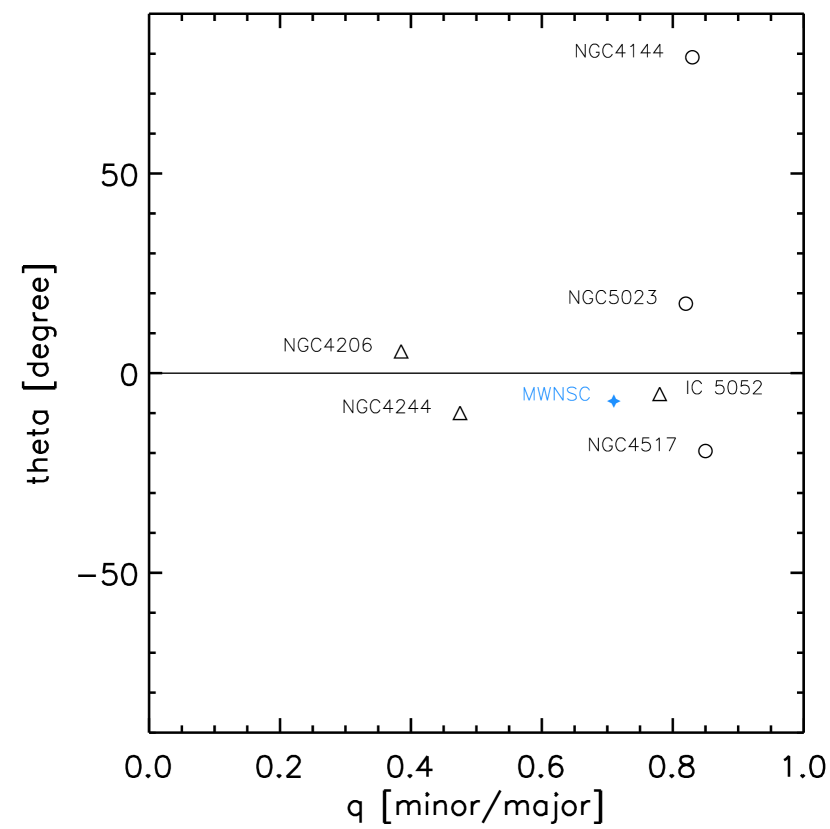
Figure 14: Axis ratio ”q” vs. ”theta”, the tilt angle between the NSC major axis and the host galaxy plane for different NSCs found in edge-on spiral galaxies (data are from Table 2 in Seth et al. 2006). The data have been averaged for the two different filters for every NSC. The name of the galaxy is indicated in the panel. The three ”multicomponent” nuclear clusters are all aligned within -10 degrees of the galactic plane of the host galaxy (triangles), similar to the value of the MWNSC found in the present study (the blue star). All the NSCs are flattened along the plane of the galaxy, similar to what is observed for the MWNSC.

5.5 Implications for the stellar cusp around Sgr A*

The formation of a stellar cusp around a massive BH in a dense and dynamically relaxed SC is a firm prediction of theoretical stellar dynamics (e.g., Lightman & Shapiro 1977; Bahcall & Wolf 1976; Freitag et al. 2006; Hopman & Alexander 2006). These latter authors reach the same conclusion using analytical, Monte Carlo, or N-body simulations: the stellar number density is described by a power law of the form $\rho\sim r^{-\gamma}$, where $r$ is the distance from the black hole and $\rho$ is the stellar density. The GC is a unique case to study the existence of a cusp: it has a SMBH embedded in a massive NSC and is the closest nucleus of a galaxy. After controversial observational studies that showed an almost flat, core-like distribution of stars close to the black hole, Gallego-Cano et al. (2018) and Schödel et al. (2018) found strong evidence of the existence of the stellar cusp around Sgr A*. Thanks to improved methodologies, these latter authors reached the faintest stars studied and tested other possible tracer populations. Their results were corroborated theoretically by Baumgardt et al. (2018), who evolved a star cluster surrounding a central massive black hole over a Hubble time under the combined influence of two-body relaxation and continuous star formation.

In order to describe the 3D shape of the cluster in detail, Gallego-Cano et al. (2018) and Schödel et al. (2018) needed to convert the measured 2D profile into a 3D density law and deal with projection effects. For this reason, they added data at projected radii $R\geq 2$ pc from the literature (Schödel et al. 2014a; Fritz et al. 2016). They used the Nuker model from Lauer et al. (1995) as a generalization of a broken power law as given in equation  1 of Fritz et al. (2016). We repeat the work of Gallego-Cano et al. (2018) and Schödel et al. (2018) (see more details in their papers) for $K_{s}\approx 18$ stars, but including new data from the GALACTICNUCLEUS survey for distances larger than $1.5$ pc to compute the Nuker fit. Moreover, we use the model for the nonNSC emission computed in the present work to subtract the GB and NSD contributions from our sample. We use the NSD Model 2 from Table 4. The resulting best-fit parameters are given in Table 11, where we explore different sources of systematics error (see Appendix B). Figure 15 shows the Nuker fit ID 10 in Table11. The black point represents the corrected surface density data for stars in the magnitude interval $17.5\leq K_{s}\leq 18.5$ from Gallego-Cano et al. (2018), complemented at large radii by scaled data from GALACTICNUCLEUS data. In order to obtain the value for the inner power-law $\gamma$ that describes the cusp, we use the mean and standard deviation of the best-fit values of Table 11 and we add the statistical systematic errors quadratically. We obtain a value of $\gamma=1.38\pm 0.06_{sys}\pm 0.01_{stat}$. As we can see, the mean parameters agree within the uncertainties with the value of $\gamma=1.43\pm 0.02\pm 0.1_{sys}$ determined in Gallego-Cano et al. (2018).

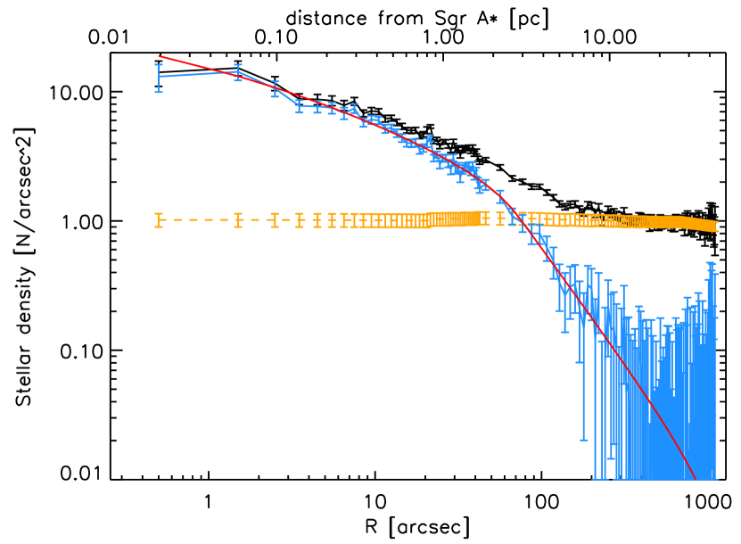
Figure 15: Black: Combined, corrected surface density data for stars in the magnitude interval $17.5\leq K_{s}\leq 18.5$ from Gallego-Cano et al. (2018), plus scaled data from the GALACTICNUCLEUS survey at large radii. The blue data points are the data after subtraction of the Model 2 in Table 4 for the emission from the nuclear stellar disk and the Galactic bulge (the dashed orange line). The red line is a Nuker model fit (ID 10 in Table 11).

5.6 Clues to the Milky Way nuclear star cluster formation

Nuclear stellar clusters may grow by in situ star formation or by the accretion of other stellar clusters formed sufficiently close to them so that they can be accreted within a Hubble time. Since the relaxation time in NSCs can be as long as a Hubble time (e.g., in the case of the MW, according to Alexander 2017), this implies that accretion or star formation events may be observable in the form of structural or dynamical peculiarities. Such peculiarities have been observed: a starburst happened a few million years ago within $0.5$ pc of the central black hole of the Milky Way (see Genzel et al. 2010, and references therein) and also some extragalactic NSCs show centrally concentrated young populations (Georgiev & Böker 2014; Carson et al. 2015). However, younger populations can also be found at greater radii in NSCs (Carson et al. 2015). Our observation of the flattened distribution of bright giants and the observation of a potential rotating substructure perpendicular to the Galactic plane at a projected radius of about 0.8 pc from the center by Feldmeier et al. (2014) indicate that dynamically unrelaxed populations may also be present at larger radii in the MWNSC. While we cannot accurately constrain the formation of the MWNSC from the existing incomplete observational data, those substructures at least provide an indication that it can grow through in situ formation and accretion of nearby clusters. To look into what mechanism plays a more important role in the formation of the MWNSC, we need higher angular resolution NIR imaging and spectroscopy in order to disentangle the different stellar populations inside the NSC.

6 Conclusions

In order to constrain the overall properties of the NSC of the Milky Way and overcome some potential shortcomings of previous studies, we analyzed two different datasets and methods. Using star count analyses of high-angular-resolution images from NACO and HAWK-I we created extinction-corrected stellar density maps for old stars. We also improved the analysis of the IRAC/Spitzer MIR images, which are less affected by extinction than those from NACO and HAWK-1. We model the Galactic bulge and the nuclear stellar disk that surround the MWNSC. We subtracted both foreground and background contributions from the MWNSC and fit Sérsic models to the images. We obtained a value of the effective radius $R_{e}=(5.1\pm 1.0)$ pc. Moreover, we found that the MWNSC is flattened, with its major axis almost parallel to the Galactic plane. The axis ratio is $q=0.71\pm 0.10$, the ellipticity is $\epsilon=1-q=0.29\pm 0.10$, and the Sérsic index is $n=2.2\pm 0.7$. The structure of the MWNSC is similar to that of other extragalactic NSCs found in spiral galaxies.

We analyzed the symmetry of the MWNSC, firstly assuming that it is aligned with respect to the Galactic plane, in agreement with previous studies, and secondly leaving the angle between the major axis of the MWNSC and the GP free to vary in the fits. We found that the major axis of the MWNSC may be tilted out of the GP by as much as -10 degrees, which is novel confirmation of the value of the angle in the kinematic position obtained by Feldmeier et al. (2014) and of the observations of NSCs from nearby galaxies.

Thanks to our high-angular-resolution images, we were able to study the structure of the MWNSC in different ranges of magnitude. We found some differences between the distributions of brighter giants and RC stars, the former being significantly more flattened. Bright giants are younger than RC stars, on average, according to stellar evolutionary models, and are expected to have bluer colors than the older ones. Furthermore, our findings are in agreement with the differences found between the effective radius of NSCs observed in nearby galaxies at different wavelengths, which may suggest that the populations of different ages are not completely mixed. The observation of the flattened distribution of bright giants may be support for the in situ star formation scenario for the MWNSC.

Finally, we studied the stellar cusp around Sgr A* using GALACTICNUCLEUS data for distances greater than $1.5$ pc and assuming our new GB and NSD models in the Nuker fit. This cusp is well developed inside the influence radius of Sgr A* and can be described by a single three-dimensional power law with an exponent $\gamma=1.38\pm 0.06_{sys}\pm 0.01_{stat}$, consistent with previous work.

Appendix A Systematic errors on the 2D fit of the stellar density maps

In this Appendix we examine some of the potential sources of systematic error in the computation of the main NSC parameters.

A.1 Extinction and completeness

As we see in the Section 3.1, we do not apply any completeness correction to the data but we mask out the pixels where the density is too low (or high) by comparing with their neighbors. Moreover, we study only the fields where the completeness is greater than 50% in the range of magnitudes considered.

In order to study the systematic uncertainty derived by the extinction correction we analyze the density map without any corrections. All the parameters that we obtain in the fits are consistent with the final results in Table 2 at the $3\sigma$ level. We repeat the procedure to study the effect on the final NSC parameters of the extinction index uncertainty from Nogueras-Lara et al. (2018b, 2019c) ($\bigtriangleup\alpha=0.08$). We use $\alpha=2.38$ and $\alpha=2.22$, respectively. The standard deviations of the NSC parameters are shown in Table 7. The final uncertainties are included in Table 2 and Table 3 by adding quadratically to the uncertainties computed in following sections. The standard deviations in the stellar number density for the NSD at its effective radius are smaller than $0.01$ in all cases. We can see that the flattening is the parameter that is least affected by this effect.

Table 7: Test of potential sources of systematic errors in the NSC parameters obtained in the Sérsic fits due to the selection of a different extinction index ($\alpha=2.22$, $\alpha=2.30$ and $\alpha=2.38$).

ID	Mag. range	$\sigma(\theta)$	$\sigma(N_{nsc})$	$\sigma(q)$	$\sigma(n)$	$\sigma(R_{e})$
	($K_{s,extc}$)	(degree)	(stars/bin2)			(pc)
1	$12.5-14$	-	$0.55$	$0.01$	$0.18$	$0.24$
2	$9-12$	-	$0.16$	$0.02$	$0.21$	$0.02$
3	$9-14$	-	$0.45$	$0.01$	$0.02$	$0.09$
4	$12.5-14$	$1.42$	$0.43$	$0.01$	$0.13$	$0.10$
5	$9-12$	$0.40$	$0.16$	$0.02$	$0.19$	$0.02$
6	$9-14$	$0.37$	$0.44$	$0.01$	$0.01$	$0.07$

We also repeat the whole procedure to create the stellar density maps by considering a less steep value for the extinction index. We use $\alpha=2.11\pm 0.06$ from Fritz et al. (2011). The best-fit parameters are consistent with the final values in Table 2 at the $1-2\sigma$ level. Although the value of $\alpha\sim 2.30$ from Nogueras-Lara et al. (2018a) that we use has been obtained for the central field ($\sim 7.95^{\prime}\times 3.43^{\prime}$), Nogueras-Lara et al. (2018b) studied other regions further out and obtained a very similar value of $\alpha$ that is within the uncertainties. Therefore, we can expect that the value of the extinction index is approximately constant for the entire FOV of our data. We conclude that extinction and completeness are not a significant source of systematic error.

A.2 Mask

In this section, we test the effect of different masks in the fits. As we explain in section 3.1, we create masks to take into account the inhomogeneity of the field of HAWK-I data. Figure  16 shows two of the masks that we applied. Masks range from less restrictive (Mask 1) to more restrictive (Mask 4). The differences between the masks are due to the selection of different values for the density thresholds to mask out regions with low density (global mask). With the local mask, we also rule out pixels with overly high density. Moreover, we also study the local mask by rejecting the points whose values are larger than 2- 3$\sigma$, but the differences between the obtained NSC parameters are negligible.

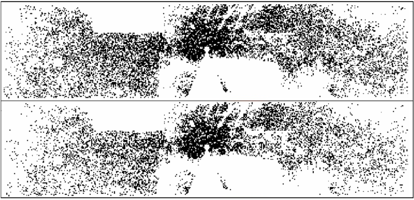
Figure 16: Masks 2 and 3 applied to the extinction-corrected stellar number density maps of the central $86$ pc $\times$ $20.2$ pc of the Galaxy. The masked regions are in white. The differences between both masks are due to the selection of two different values for the density thresholds to mask out regions with low density. Galactic north is up and Galactic east is to the left. The Galactic plane runs horizontally.

Table 8 shows all the results for masks 1, 2, 3, and 4. The uncertainties are the standard deviations of the best-fit parameters. The selection of the mask is an important source of systematic error that we have already considered in Table 2.

Table 8: Test of potential sources of systematic errors in the NSC parameters obtained in the Sérsic fits due to the selection of the masks. The MWNSC is aligned with respect to GP.

ID	Mag. range	Mask	$N^{b}_{e,nsd}$	$N^{c}_{e,nsc}$	$q^{d}$	$n^{e}$	$R^{f}_{e}$
	($K_{s,extc}$)		(stars/bin2)	(stars/bin2)			(pc)
1	$12.5-14$	$3$	$2.39\pm 0.01$	$3.49\pm 0.27$	$0.83\pm 0.01$	$2.73\pm 0.11$	$5.83\pm 0.28$
2	$12.5-14$	$4$	$2.57\pm 0.01$	$3.86\pm 0.28$	$0.79\pm 0.01$	$2.73\pm 0.10$	$5.42\pm 0.24$
3	$12.5-14^{a}_{sym}$	$1$	$2.36\pm 0.01$	$4.32\pm 0.19$	$0.89\pm 0.01$	$2.38\pm 0.07$	$5.68\pm 0.15$
4	$12.5-14^{a}_{sym}$	$2$	$2.49\pm 0.01$	$4.09\pm 0.20$	$0.87\pm 0.01$	$2.52\pm 0.07$	$5.73\pm 0.17$
5	$9-12$	$3$	$0.47\pm 0.00$	$1.25\pm 0.13$	$0.59\pm 0.01$	$2.22\pm 0.17$	$3.92\pm 0.23$
6	$9-12$	$4$	$0.49\pm 0.00$	$1.21\pm 0.13$	$0.56\pm 0.01$	$2.25\pm 0.17$	$4.09\pm 0.25$
7	$9-12^{a}_{sym}$	$1$	$0.61\pm 0.01$	$1.26\pm 0.09$	$0.62\pm 0.01$	$2.04\pm 0.11$	$4.68\pm 0.19$
8	$9-12^{a}_{sym}$	$2$	$0.64\pm 0.01$	$0.91\pm 0.09$	$0.61\pm 0.01$	$2.61\pm 0.16$	$5.61\pm 0.35$
9	$9-14$	$3$	$3.23\pm 0.01$	$5.52\pm 0.28$	$0.78\pm 0.01$	$2.43\pm 0.07$	$5.54\pm 0.17$
10	$9-14$	$4$	$3.46\pm 0.01$	$5.99\pm 0.28$	$0.75\pm 0.01$	$2.40\pm 0.06$	$5.20\pm 0.15$
11	$9-14^{a}_{sym}$	$1$	$2.99\pm 0.01$	$7.52\pm 0.16$	$0.80\pm 0.01$	$1.60\pm 0.03$	$5.40\pm 0.07$
12	$9-14^{a}_{sym}$	$2$	$3.19\pm 0.01$	$7.17\pm 0.16$	$0.79\pm 0.01$	$1.63\pm 0.03$	$5.37\pm 0.07$

We test the systematic errors associated with the selection of the masks for the fits where we leave the tilt angle between the NSC and the GP free to vary. This is an important source of systematic error that we have already considered in Table 3, which shows all the obtained results. The parameters do not show a systematic behavior if we apply a more restrictive mask.

Table 9: Test of potential sources of systematic error in the NSC parameters obtained in the Sérsic fits due to the selection of the masks. The tilt angle $\theta$ between the NSC and the GP is a free parameter in the fits.

ID	Mag. range	Mask	$\theta^{b}$	$N_{e,NSD}$	$N_{e,NSC}$	$q$	$n$	$R_{e}$
	($K_{s,extc}$)		(degree)	(stars/bin2)	(stars/bin2)			(pc)
1	$12.5-14$	$3$	$-8.50\pm 1.03$	$2.39\pm 0.01$	$3.53\pm 0.26$	$0.82\pm 0.01$	$2.70\pm 0.10$	$5.83\pm 0.26$
2	$12.5-14$	$4$	$-8.52\pm 0.83$	$2.56\pm 0.01$	$3.87\pm 0.28$	$0.77\pm 0.01$	$2.71\pm 0.10$	$5.45\pm 0.24$
3	$12.5-14^{a}_{sym}$	$1$	$-8.51\pm 0.00$	$2.32\pm 0.01$	$3.18\pm 0.24$	$0.87\pm 0.01$	$3.20\pm 0.14$	$6.69\pm 0.30$
4	$12.5-14^{a}_{sym}$	$2$	$-8.51\pm 0.00$	$2.45\pm 0.01$	$2.92\pm 0.25$	$0.87\pm 0.01$	$3.43\pm 0.16$	$6.80\pm 0.35$
5	$9-12$	$3$	$-5.65\pm 0.87$	$0.47\pm 0.01$	$1.33\pm 0.12$	$0.57\pm 0.01$	$2.06\pm 0.15$	$3.85\pm 0.20$
6	$9-12$	$4$	$-5.56\pm 0.74$	$0.49\pm 0.01$	$1.28\pm 0.12$	$0.54\pm 0.01$	$2.12\pm 0.15$	$4.04\pm 0.23$
7	$9-12^{a}_{sym}$	$1$	$-5.60\pm 0.00$	$0.60\pm 0.01$	$1.26\pm 0.07$	$0.75\pm 0.01$	$1.67\pm 0.08$	$4.42\pm 0.15$
8	$9-12^{a}_{sym}$	$2$	$-5.60\pm 0.00$	$0.63\pm 0.01$	$1.08\pm 0.08$	$0.71\pm 0.01$	$1.87\pm 0.10$	$4.94\pm 0.22$
9	$9-14$	$3$	$-7.47\pm 0.60$	$3.23\pm 0.01$	$5.60\pm 0.27$	$0.76\pm 0.01$	$2.39\pm 0.07$	$5.53\pm 0.16$
10	$9-14$	$4$	$-6.49\pm 0.54$	$3.45\pm 0.01$	$5.92\pm 0.27$	$0.74\pm 0.01$	$2.40\pm 0.06$	$5.27\pm 0.15$
11	$9-14^{a}_{sym}$	$1$	$-6.98\pm 0.01$	$2.96\pm 0.00$	$6.88\pm 0.25$	$0.75\pm 0.01$	$2.23\pm 0.07$	$5.69\pm 0.12$
12	$9-14^{a}_{sym}$	$2$	$-6.98\pm 0.01$	$3.18\pm 0.00$	$8.14\pm 0.23$	$0.74\pm 0.01$	$2.00\pm 0.05$	$4.97\pm 0.08$

A.3 Inner mask

In this section, we examine several potential sources of systematic error in the NSC parameters due to masking different central regions around Sgr A*. In order to explore the systematic errors, we test the effects of masking the central $0.4$ pc, $0.6$ pc, and $0.8$ pc, respectively. Table 10 shows the results. The final uncertainties are included in Tables 2 and 3 by adding quadratically to the uncertainties due to the selection of the mask computed in the previous section.

Table 10: Test of potential sources of systematic errors in the NSC parameters obtained in the Sérsic fits due to masking the inner $0.4$ pc, $0.6$ pc, and $0.8$ pc, respectively, around Sgr A*. We only show the parameters of the magnitude ranges that are significantly affected.

ID	Mag. range	$\theta^{b}$	$\sigma(\theta)$	$N_{nsc}$	$\sigma(N_{nsc})$	$n$	$\sigma(n)$	$R_{e}$	$\sigma(R_{e})$
	($K_{s,extc}$)	(degree)	(degree)	(stars/bin2)	(stars/bin2)			(pc)	(pc)
1	$12.5-14$	0	-	$3.84,3.86,3.66$	$0.11$	$2.75,2.73,2.86$	$0.07$	$5.44,5.42,5.57$	$0.08$
2	$9-12$	0	-	$1.11,1.21,1.35$	$0.12$	$2.53,2.25,1.85$	$0.34$	$4.22,4.09,3.92$	$0.15$
3	$9-14$	0	-	$5.78,5.99,6.24$	$0.23$	$2.47,2.40,2.33$	$0.07$	$5.30,5.20,5.06$	$0.12$
4	$12.5-14$	$-5.5,-8.5,-10.8$	$2.6$	$3.84,3.87,3.96$	$0.06$	$2.73,2.71,2.69$	$0.02$	$5.47,5.45,5.38$	$0.05$
5	$9-12$	$-3.8,-5.6,-6.2$	$1.2$	$1.18,1.28,1.48$	$0.15$	$2.42,2.12,1.61$	$0.41$	$4.14,4.04,3.82$	$0.16$
6	$9-14$	$-5.6,-6.5,-7.3$	$0.9$	$5.75,5.92,6.33$	$0.30$	$2.47,2.40,2.28$	$0.09$	$5.34,5.27,5.06$	$0.14$

A.4 Spatial binning

We analyzed the results considering different ways of spatially binning the data. Firstly, we studied the optimal bin size for our density maps following the studies of Knuth (2006) and Witzel et al. (2012). These latter authors applied Bayesian probability theory to develop a straightforward algorithm to compute the posterior probability of bins for a given data set (see more details in their papers). We limit our sample to the stars brighter than $K_{s}=16.0$. The dependence of the relative logarithmic posterior probability (RLP) on the bin number is shown in Fig. 17. The maximum for the RLP for the star number is reached for 147 bins, and the best bin size is $7^{\prime\prime}$. Secondly, in order to smooth the overlapping region between data of different resolution, we test other smaller values of binning of $5^{\prime\prime}$ and $6^{\prime\prime}$, obtaining the values for the maximum of the RLP of 195 and 172, respectively. In figure 17, we can see that the value of the RLP is very similar for those values. Regardless, we study our results by selecting a bin size of $7"\times 7"$ and we obtain all the values for the NSC parameters consistent with the final results in Table 2 at the 2$\sigma$ level. We select a bin size of $5"\times 5"$ because it is better suited to our data and allows us to study the major features at the large scale of the NSC with enough detail without taking into account the random fluctuations. We conclude that spatial binning is not a significant source of systematic error in our analysis.

Figure 17: Optimal spatial binning. We show the RLP as a function of the number of bins. The maximum for the RLP is reached for 147 bins (red line). The values for 172 bins (green line) and 195 bins (blue line) are obtained for bin sizes of $6^{\prime\prime}$ and $5^{\prime\prime}$ , respectively. We study all stars brighter than $K_{s}=16.0$

A.5 Edges between NACO and HAWK-I

As we saw in section 3, we compute the mean density at the edges between HAWK-I and NACO data with an outer radius of around $1.5$ pc and inner radius of around $1.3$ pc (see Fig. 3). We explore the sources of systematic error associated with the size of the edges that we choose. We test different values for the inner radius ($1.2$ pc and $1.4$ pc, respectively). The differences between the obtained NSC parameters and the values in Table 2 are negligible.

A.6 Contamination by stars in the GD

We removed the contribution of NSD and GB in the NSC fits. We also explored the effect of excluding foreground stars from the GD based on their color H - K_s. If we do not consider stars with $H-K_{s}<1.2$, the best-fit parameters are consistent with the final values in Table 2 at the $1\sigma$ level. Therefore, contamination from stars in the GD was found to have no significant impact on the results. In addition, some of the excluded stars may be part of the GB or NSD and we have already taken them into account; we therefore prefer not to apply this correction.

A.7 Magnitude cut

In order to study the RC distribution, we considered stars with K_s up to 16 (K${}_{s,extc}\sim 14.0$), as can be seen in the K_s-luminosity function from Fig.  3. However, we analyzed the fits obtained when creating the density maps considering a magnitude cut of K${}_{s}=15.5$ before the extinction correction. All the values for the NSC parameters are consistent with the final results in Table 2 at the $2\sigma$ level.

A.8 Saturation of stars

We select the brightest magnitude in the range of the stars to be not significantly affected by saturation in the images. For HAWK-I data, stars with $K_{s}\sim 11.0$ ($K_{s,extc}\sim 9.0$) are saturated. We selected the bright limit of $K_{s}=11.0$ ($K_{s,extc}=9.0$) in our analysis, but we also explored the effects of using another bright limit, $K_{s}=10.0$ ($K_{s,extc}=8.0$). The differences in the NSC parameters that we obtain from using these two limits are very small ($\Delta Re<3.1$%, $\Delta n<2.5$%, and $\Delta q<0.7$%).

A.9 Possible contamination from young stars

We aim to study the structure of the relaxed stars in the NSC. We know that a star formation event created on the order of $10^{4}$ M_⊙ of young stars in the $\sim$ 0.5 pc region around Sgr A* (Bartko et al. 2010; Lu et al. 2013; Feldmeier-Krause et al. 2015). As we see in section 3, we exclude all spectroscopically identified early-type stars from our sample (using the data of Do et al. 2013). In addition, 90% of the young stars found in Feldmeier-Krause et al. (2015) are identified within $0.5$ pc; therefore, further out we do not expect important contamination from young stars in our sample. We apply an inner mask to the $0.6$ pc region around Sgr A*. We conclude that the contamination of young stars in our data is not significant.

A.10 Initial tilt angle

In this section, we focus on the sources of systematic error that affect the possible tilt angle ($\theta$) between the NSC and the GP obtained in the fits. We have studied the effect of the mask in the previous section. In this section, we explore the systematic errors associated with the selection of different initial $\theta$ when performing the fit. As we see in previous sections, in order to find the best-fit parameters, we use the IDL MPCURVEFIT procedure that performs a Levenberg-Marquardt least-squares fit. The algorithm finds the local minimum that minimizes the chi-square, which is not the global minimum in most cases. We compare the average of the residuals obtained by subtracting the symmetrized maps from the images (see Fig 10) and we find multiple minima for different tilt angles. For this reason, it is very important to provide an initial guess for $\theta$ close to the final solution in order to obtain the global minimum. Figure 18 shows the best-fit tilt angles versus different initial values of the angle for the different magnitude ranges. The median values are indicated in the plots. The errors are the average deviation from the median. We reject data more than $3\sigma$ from the median. We conclude that the initial $\theta$ is a significant source of systematic error in our analysis and we include them in our final budget in Table 3.

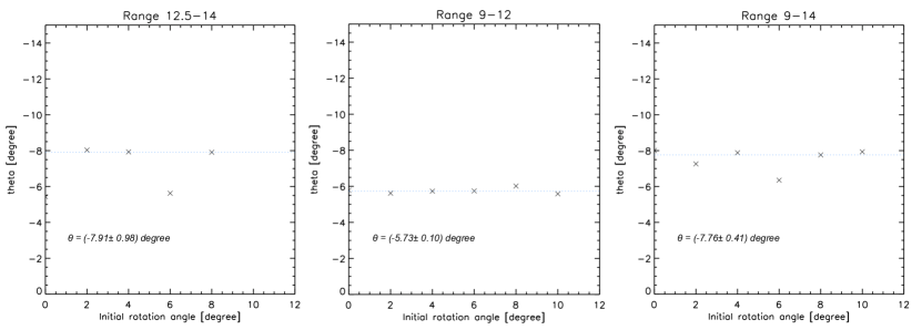
Figure 18: Mean values of the best-fit tilt angles ($\theta$) for the different magnitude ranges obtained from the fits by considering different initial values. The dotted blue line indicates the median $\theta$ and their values are shown in the different panels.

Appendix B Systematic errors of the inner power-law index

In this section, we examine several potential sources of systematic error in the computation of the power-law indices for the fits of the 3D density. We only focus on the possible systematic error due to the computation of the star density at large distances using data from the present work. Table 11 shows the best-fit parameters for the break radius $r_{b}$, for the exponents of the inner, $\gamma$, and the outer, $\beta$ power-law. We test two ways of binning the data (5 arcsec and 10 arcsec, respectively), use two different masks, and assume two different ranges of magnitudes for the stars that we select (bright and faint stars). Finally, we compute the density along the GP in a strip $\pm 50^{\prime\prime}$ and azimuthally averaged in annuli around Sgr A*.

Table 11: Best-fit model parameters for Nuker fits.

ID	Mag. range	Mask	Bin size	$r_{b}$	$\gamma$	$\beta$	$\chi^{2}_{reduced}$
	($K_{s,extc}$)		(arcsec)	(pc)
1a	$12.5-14$	$3$	$10$	$1.99\pm 0.19$	$1.34\pm 0.05$	$2.64\pm 0.10$	$1.39$
2a	$12.5-14$	$4$	$10$	$1.97\pm 0.20$	$1.34\pm 0.05$	$2.70\pm 0.12$	$1.16$
3a	$12.5-14$	$3$	$5$	$1.86\pm 0.12$	$1.30\pm 0.05$	$2.75\pm 0.08$	$1.30$
4a	$9-12$	$3$	$10$	$2.23\pm 0.47$	$1.45\pm 0.05$	$2.38\pm 0.16$	$0.64$
5a	$9-12$	$4$	$10$	$2.04\pm 0.45$	$1.44\pm 0.05$	$2.33\pm 0.15$	$0.51$
6a	$9-12$	$3$	$5$	$2.11\pm 0.32$	$1.44\pm 0.04$	$2.51\pm 0.14$	$0.70$
7b	$12.5-14$	$3$	$10$	$2.04\pm 0.15$	$1.33\pm 0.05$	$2.81\pm 0.08$	$1.82$
8b	$12.5-14$	$4$	$10$	$2.00\pm 0.15$	$1.32\pm 0.05$	$2.86\pm 0.10$	$1.60$
9b	$12.5-14$	$3$	$5$	$1.95\pm 0.11$	$1.30\pm 0.05$	$2.93\pm 0.07$	$1.67$
10b	$9-12$	$3$	$10$	$2.67\pm 0.37$	$1.44\pm 0.04$	$2.80\pm 0.19$	$1.00$
11b	$9-12$	$4$	$10$	$2.63\pm 0.39$	$1.44\pm 0.04$	$2.87\pm 0.23$	$0.85$
12b	$9-12$	$3$	$5$	$2.54\pm 0.25$	$1.42\pm 0.04$	$3.01\pm 0.18$	$0.96$