Model Reuse with Reduced
Kernel Mean Embedding Specification
Abstract
Given a publicly available pool of machine learning models constructed for various tasks, when a user plans to build a model for her own machine learning application, is it possible to build upon models in the pool such that the previous efforts on these existing models can be reused rather than starting from scratch? Here, a grand challenge is how to find models that are helpful for the current application, without accessing the raw training data for the models in the pool. In this paper, we present a two-phase framework. In the upload phase, when a model is uploading into the pool, we construct a reduced kernel mean embedding (RKME) as a specification for the model. Then in the deployment phase, the relatedness of the current task and pre-trained models will be measured based on the value of the RKME specification. Theoretical results and extensive experiments validate the effectiveness of our approach.
1 Introduction
Recently, the learnware [Zhou, 2016] paradigm has been proposed. A learnware is a well-performed pre-trained machine learning model with a specification which explains the purpose and/or specialty of the model. The provider of a learnware can upload it to a market, and ideally, the market will be a pool of (model, specification) pairs solving different tasks. When a person is going to tackle her own learning task, she can identify a good or some useful learnwares from that market whose specifications match her requirements and apply them to her own problem.
One of the most important properties of learnware is to enable future users to build their own applications upon previous models without accessing the raw data used to train these models, and thus, the machine learning experience is shared but the data privacy violation and data improper disclosure issues are avoided. This property is named inaccessibility of training data.
Note that it may be too optimistic to expect that there is a model in the pool which was trained exactly for the current task; maybe there is one, or multiple, or even none helpful models. Thus, a key challenge is how to provide each model with a specification such that given a new learning task, it is possible to identify helpful models from the model pool. This property is named reusability of pre-trained models.
It was thought that logical clauses or some simple statistics may be used to construct the model specification [Zhou, 2016], though there has been no effective approach yet. In this paper, we show that it is possible to construct a reduced kernel mean embedding (RKME) specification for this purpose, where both inaccessibility and reusability are satisfied under reasonable assumptions.
Kernel mean embedding [Muandet et al., 2017] is a powerful technique for solving distribution-related problems, and has made widespread contribution in statistics and machine learning, like two-sample testing [Jitkrittum et al., 2016], casual discovery [Doran et al., 2014], and anomaly detection [Muandet and Schölkopf, 2013]. Roughly speaking, KME maps a probability distribution to a point in reproducing kernel Hilbert space (RKHS), and can be regarded as a representation of distribution. Reduced set construction [Schölkopf et al., 1999] keeps the representation power of empirical KMEs, and blocks access to raw data points at the same time.
To clearly show why reduced KME is a valid specification in the learnware paradigm, we decompose the paradigm into a two-phase framework. Initially, in the upload phase, the pre-trained model provider is required to construct a reduced set of empirical KME as her model’s specification and upload it together with the built predictive model into a public pool. The RKME represents the distribution of model’s training data, without using any raw examples. Subsequently, in the deployment phase, we demonstrate that the user can select suitable pre-trained model(s) from the pool to predict her current task by utilizing the specifications and her unlabeled testing points in a systematic way.
RKME specification is a bridge between the current task and solved tasks upon which the pre-trained models are built. We formalize two possible relationships between the current and the solved tasks. The first one is task-recurrent assumption, saying the data distribution of the current task matches one of the solved tasks. We then use the maximum mean discrepancy (MMD) criteria to find the unique fittest model in the pool to handle all testing points. The second one is instance-recurrent assumption, saying the distribution of the current task is a mixture of solved tasks. Our algorithm estimates the mixture weight, uses the weight to generate auxiliary data mimicking the current distribution, learns a selector on these data, then uses the selector to choose the fittest pre-trained model for each testing point. Kernel herding [Chen, 2013], a fast sampling method for KME, is applied in mimic set generation.
Our main contributions are:
-
•
Propose using RKME as the specification under the learnware paradigm, and implement a two-phase framework to support the usage.
-
•
Show the inaccessibility of training data in the upload phase, i.e., no raw example is exposed after constructing specifications.
-
•
Prove the reusability of pre-trained models in the deployment phase, i.e., the current task can be handled with identified existing model(s).
-
•
Evaluate our proposal through extensive experiments including a real industrial project.
In the following sections, we first present necessary background knowledge, then introduce our proposed framework, followed by theoretical analysis, related work, experiments and finally the conclusion.
2 Background
In this section, we briefly introduce several concepts and techniques. They will be incorporated and further explained in detail through this paper.
2.1 Kernel Mean Embeddings
Let be a random variable in and be a measurable probability function of . Let be reproducing kernels for , with associated RKHS and , the corresponding canonical feature maps on . Throughout this paper, we assume the kernel function is continuous, bounded, and positive-definite. The kernel function is considered a similarity measure on a pair of points in .
Kernel mean embedding (KME) [Smola et al., 2007] is defined by the mean of a -valued random variable that maps the probability distributions to an element in RKHS associated with kernel [Schölkopf and Smola, 2002]. Denote the distribution of an -valued random variable by , then its kernel mean embedding is
| (1) |
By the reproducing property, , which demonstrates the notion of mean.
By using characteristic kernels [Fukumizu et al., 2007], it was proved that no information about the distribution would be lost after mapping to . Precisely, is equivalent to . This property makes KME a theoretically sound method to represent a distribution. An example of characteristic kernel is the Gaussian kernel
| (2) |
In learning tasks, we often have no access to the true distribution , and consequently to the true embedding . Therefore, the common practice is to use examples , which constructs an empirical distribtuion , to approximate (1):
| (3) |
If all functions in are bounded and examples are i.i.d drawn, the empirical KME converges to the true KME at rate , measured by RKHS norm [Lopez-Paz et al., 2015, Theorem 1].
2.2 Reduced Set Construction
Reduced set methods were first proposed to speed up SVM predictions [Burges, 1996] by reducing the number of support vectors, and soon were found useful in kernel mean embeddings [Schölkopf et al., 1999] to handle storage and/or computational difficulties.
The empirical KME is an approximation of true KME , requiring all the raw examples. It is known that we can approximate the empirical KME with fewer examples. Reduced set methods find a weighted set of points in the input space to minimize the distance measured by RKHS norm
| (4) |
It is trivial to achieve perfect approximation if we are allowed to have the same number of points in the reduced set (). Therefore we focus on the case by introducing additional freedom on real-value coefficients and vectors . If points in are selected from , it is called reduced set selection. Otherwise, if are newly constructed vectors, it is called reduced set construction [Arif and Vela, 2009]. Since the latter does not expose raw examples, we apply reduced set construction to compute the specification in the upload phase of our proposal.
2.3 Kernel Herding
Kernel herding algorithm is an infinite memory deterministic process that learns to approximate a distribution with a collection of examples [Chen et al., 2010]. Suppose we want to draw examples from distribution , but the probability distribution function of is unknown. Given the kernel mean embedding of , assume is bounded for all and the further restrictions of finite-dimensional discrete state spaces [Welling, 2009], kernel herding will iteratively draw an example in terms of greedily reducing the following error at every iteration:
| (5) |
A remarkable result of kernel herding is, it decreases the square error in (5) at a rate , which is faster than generating independent identically distributed random samples from at a rate .
Comparing with (4) in last section, if we set , kernel herding looks like an “inverse” operation of reduced set construction. Reduce set construction in (4) is “compressing” the KME, while kernel herding in (5) is “decompressing” the information in reduced KME if is large. We will apply kernel herding in the deployment phase to help recover the information in reduced KMEs.
3 Framework
In this section, we first formalize our problem setting with minimal notations, then show how to construct RKME in the upload phase and how to use RKME in the deployment phase.
3.1 Problem Formulation
Suppose there are in total providers in the upload phase, they build learnwares on their own tasks and generously upload them to a pool for future users. Each of them has a private local dataset , which reflects the task . Task is a pair defined by a distribution on input space and a global optimal rule function ,
| (6) |
All providers are competent, and the local datasets are sufficient to solve their tasks. Formally speaking, their models enjoy a small error rate with respect to a certain loss function on their task distribution :
| (7) |
With a slight abuse of notation, here can be either a regression loss or classification loss. Since tasks are equipped with low-error pre-trained models, they are referred to as solved tasks throughout this paper.
In the deployment phase, a new user wants to solve her current task with only unlabeled testing data . Thus her mission is to learn a good model which minimizes , utilizing the information contained in pre-trained models .
This problem seems easy at the first glance. A naive reasoning is: since all the solved tasks share the same rule function , and each is a low-error estimate of , any of them is a good candidate for . However, this is not the case because no assumption between and has been made so far. In an extreme case, the support of may not be covered by the union support of , therefore there exist areas where all ’s can fail.
Put it in a concrete example. The global rule function is a 4-class classifier . There are two providers equipped with very “unlucky” distribution. One’s local dataset only contains points with two classes , and another only sees points labeled . They learn zero-error local classifiers , which are perfect for their own task and uploaded to the public pool. Then in the deployment phase facing current task , suppose all points drawn from are actually labeled class according to . In this unfortunate case, both pre-trained models suffer from 100% error on .
The above example demonstrates that it is difficult to have a low-risk model on the current task without making any assumptions on . To this end, we propose two realistic assumptions to model relationships between the current and solved tasks.
Task-recurrent assumption: The first type of assumption is that the distribution of the current task matches one of the solved tasks. The current task is said to be task-recurrent from the solved tasks if there exists , such that .
Instance-recurrent assumption: The second type of assumption is that the distribution of the current task is a convex mixture of solved tasks, i.e. , where lies in a unit simplex.
The second assumption is weaker as task-recurrent is a special case for instance-recurrent by setting at a vertex of the unit simplex. However, if we are told that the first assumption holds a priori, it is expected to achieve better performance on the current task.
3.2 Upload Phase
In this section, we describe how to compute the reduced KME specification to summarize provider ’s local dataset in the upload phase. To lighten the notations, we focus on one provider and temporarily drop the subscript .
Given a local dataset , where . Now we use empricial KME to map the empirical distribution defined by with a valid kernel function . The empirical KME is as defined in (3).
Then our mission is to find the reduced set minimizing (4). Denote and , expanding (4) gives
| (8) |
We adopt the alternating optimization to minimize (8).
Fix update . Suppose vectors in are fixed, setting obtains the closed-form solution of :
| (9) |
where
Fix update . When is fixed, in are independent in (8), therefore we can iteratively run gradient descent on each as
| (10) |
The optimization is summarized in Algorithm 1. If the step size is small, the objective value will decrease monotonically at both steps, and finally converges.
After the optimization, each provider uploads her model , paired with RKME specification (represented by and ), into the learnware pool. Raw data examples are inaccessible after the construction by design. Differential privacy can be further ensured by applying techniques in Balog et al. [2018], which is an interesting issue but out of our scope.
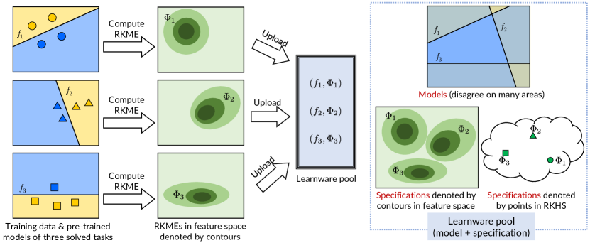
An illustration of this phase is presented in Fig. 1. In this illustration, 3 providers upload pre-trained binary classification models and computed RKMEs into the public learnware pool. They are unaware of each other, and their pre-trained models disagree on many areas. The RKMEs () are score functions in the raw feature space (denoted by contours, deeper means higher), and also points in the RKHS (denoted by points in a cloud). There is no optimal way to ensemble these models, but the RKME specifications allow future users to appropriately reuse them in the deployment phase.
3.3 Deployment Phase
In this section, we describe how to use RKME to identify useful models in the learnware pool for the current task. Algorithm 2 shows the overall deployment procedure. As we mentioned in Section 3.1, the procedure treats two different recurrent assumptions separately.
3.3.1 Task-recurrent assumption
When the task-recurrent assumption holds, which means the current distribution matches one of the distributions solved before, our goal is to find out which one fits the best. In Line 3 of Algorithm 2, we measure the RKHS distance between the testing mean embedding and reduced embeddings in the pool, and figure out the model which was trained on the closest data distribution. Then in Line 4, we apply the matching model to predict all the points.
3.3.2 Overview of instance-recurrent assumption
When the instance-recurrent assumption holds, which means no single pre-trained model can handle all the testing points, our goal is to determine which model is the most suitable for each instance. The general idea is that we “mimic” the test distribution by weighting existing distributions first, then “recover” enough data points and learn a model selector on them. Finally, the selector predicts the suitable model for each testing point.
3.3.3 Estimate mixture weights
3.3.4 Sampling from RKME
This subsection explains how to implement Line 11 of Algorithm 2, i.e., sample examples from the distribution with the help of RKME , by applying kernel herding techniques [Chen et al., 2010].
For ease of understanding, we temporarily drop the subscript , slightly abuse the notation as the iteration number here, and rewrite the iterative herding process in Chen [2013] via our notations:
| (13) |
where is the next example we want to sample from when have been already sampled. And Proposition 4.8 in Chen [2013] shows the following error will decrease as :
3.3.5 Final predictions and illustrations
When all the previous steps are ready, it is quite easy to make the final prediction. The user will train a selector on to predict which pre-trained model in the pool should be selected. The selector can be similar to pre-trained models except that its output space is the index of providers. The final prediction for a test instance will be , where is the selected index.
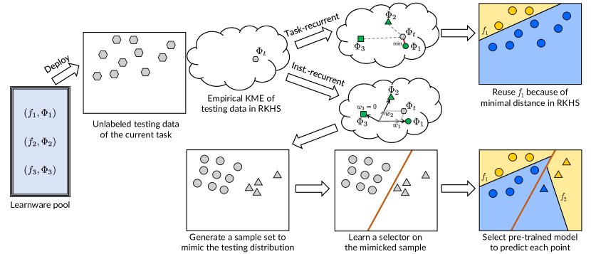
An illustration of the deployment phase including both task-recurrent and instance-recurrent assumptions is presented in Fig. 2. It is easier to see the differences between assumptions in the RKHS plotted as a cloud. If task-recurrent, we are finding the closest RKME (which is in that cloud) and only one pre-trained model will be used. If instance-recurrent, we are finding a combination of RKMEs (which is in that cloud). Each is like a basis in the reproducing kernel Hilbert space, and instance-recurrent assumption is actually saying that can be decomposed by these bases. In that example, because , more circles are generated than triangles in the mimicked sample. There is no square because . The learned selector shows we should use in the left half and in the right half.
Since we are reusing pre-trained models without modifying them on the current task, our framework accepts any types of model from providers. They can be deep neural classifiers, SVMs with different kernel functions, or gradient boosted tree regressors. As long as the input spaces are identical, these pre-trained models can even have different output spaces.
4 Theory
In this section, theoretical results are presented to rigorously justify the reusability of pre-trained models by using RKME specifications via our proposed way, either in task-recurrent assumption or in instance-recurrent assumption.
4.1 Task-recurrent
Here we introduce useful propositions regarding MMD and then show the guarantees for the task-recurrent assumption. For simplicity, we omit the subscript in and represent as .
Proposition 1 (Upper bound for empirical MMD).
We then know that when task-recurrent assumption is satisfied, the empirical MMD is bounded by a small value. Using such an idea, we further bound the empirical estimation of the task-recurrent case.
Theorem 1 (Task-recurrent bound).
Assume is task-recurrent, i.e. . The learned model from each solved task satisfy (7). Assume the loss function , and upper bounded . The empirical MMD between distribution and current distribution can be estimated from
where . Further assume that the minimum empirical MMD is bounded above: . The selected model for current task is s.t.
The finite sample loss satisfies:
| (14) |
where as .
Proof 1.
When task-recurrent assumption holds, our method either correctly identifies the recurrent pre-trained model or not. Let be the correct recurrent index. If , the result follows directly from (7). If , the loss function is
We then can represent the error of each model in the form of KME. For the current task :
since and the selected model . However, the correct matching should be . Hence, we are applying model on distribution . The empirical loss in is:
We then bound and separately.
by (7) and convergence rate for empirical MMD.
To see the bound for empirical embeddings,
the first term is by assumption and the second term is because :
which completes the proof.
The theorem shows that, in the task-recurrent setting, the test error from our procedure is bounded by the solved task error and the approximation error of empirical KME.
4.2 Instance-recurrent
In this subsection, we present the guarantee of our proposal when instance-recurrent assumption holds. Our analysis is based on the following four steps:
-
1.
The estimation of is close to the true mixture weight .
-
2.
The quality of the mimicked sample set generated by kernel herding is good.
-
3.
The error of the learned selector is bounded.
-
4.
The error of our estimated predictor is bounded.
Lemma 1 (-estimation bound).
Consider the weights estimation procedure stated in (12): where
and consider the population embedding for where
Assume is non-degenerate, i.e. the smallest eigenvalue is bounded below by a positive real number . Then,
Proof.
The proof starts from the instance-recurrent assumption where . Rewrite
| (15) | ||||
| (16) | ||||
| (17) |
(15) goes to since is a -consistent estimator of . Let . . As , we have . As is bounded, . , where as bounded of RKHS, as is non-degenerate and
as . By such construction, we are able to see the difference, in terms of Frobenius norm, of the weight vector learned from true embedding versus from empirical embedding . ∎
To better understand the instance-recurrent case, for the mixture model in (11), we perceive the component assignment as a latent variable, . Hence, by setting as the conditional distribution of given that comes from the -th component, we can write the distribution of test data as:
where is the marginal distribution of component assignment variable . This corresponds to partition weights , where . We call the the joint distribution of random variable pair .
Proposition 2.
[Chen et al., 2010, Proposition 4] Let be the target distribution, be the number of samples generated from kernel herding, and be the empirical distribution from samples. For any , the error . Moreover this condition holds uniformly, that . Thus .
The proof can be found in Chen et al. [2010], utilizing Koksma Hlawka inequality. Proposition 2 shows that the convergence rate of empirical embedding from kernel herding is which is faster than the convergence rate between empirical mean embedding to the population version from empirical samples. Hence, sampling does not make the convergence rate, from to slower.
Learning classifier from samples:
With the samples generated from the herding step, we train a selector via the following loss
We do not have direct access to as the selector is learned from the generated empirical samples. We assume the loss and thus bounded, and the training loss is small, i.e. for .
Lemma 2.
Let optimal selector and ; let the estimated embedding from the deployment phase and (12) be . Then, the population loss using the learned classifier is
Proof.
Let be herding samples from . Then
Note that is a bounded function that only depends on , as and both represent the joint distribution of . Alternatively, for discrete random variable that is finite, it is equivalent to see the embedding as where is the linear kernel w.r.t. .
Theorem 2 (Instance-recurrent bound).
Assume for the source models,
where and bounded; the classification error of trained classifier is small, i.e. , where and bounded. We further assume a Lipschitz condition between the loss used for task and the loss used for training classifier : for some . Then the RKME estimator satistifies
Proof.
The samples approximating are generated from estimated mean embedding via herding. Applying the result in Lemma 1 and Lemma 2, are -consistent and assignment error is -consistent, for .
where . The third last inequality holds as we are looking into the set where the component assignment are mis-classified. Using the Lipschitz condition, we bounded the loss using training loss results of . The second last inequality dropping holds because is non-negative loss function. By Lemma 2, the last inequality holds. ∎
5 Related Work
Domain adaptation [Sun et al., 2015] is to solve the problem where the training examples (source domain) and the testing examples (target domain) are from different distributions. A common assumption is the examples in source domain are accessible for learning the target domain, while learnware framework is designed to avoid the access at test time. Domain adaptation with multiple sources [Mansour et al., 2008; Hoffman et al., 2018] is related to our problem setting. Their remarkable theoretical results clearly show that given the direct access to distribution, a weighted combination of models can reach bounded risk at the target domain, when the gap of distributions are bounded by Rényi divergence [Mansour et al., 2009]. Compared with the literature, it is the first time that the prediction is made from dynamic selection, which is capable of eliminating useless models and more flexible for various types of model. Furthermore, density estimation is considered difficult in high dimensional space, while ours does not depend on estimated density function but implicitly matching distributions via RKME for model selection.
Data privacy is a common concern in practice. In terms of multiple participants setting like ours, multiparty learning [Pathak et al., 2010], and recently a popular special case called federated learning [Yang et al., 2019; Konečný et al., 2016] are related. Existing approaches for multiparty learning usually assume the local dataset owner follows a predefined communication protocol, and they jointly learn one global model by continuously exchanging information to others or a central party. Despite the success of that paradigm such as Gboard presented in Hard et al. [2018], we observe that in many real-world scenarios, local data owners are unable to participate in such an iterative process because of no continuous connection to others or a central party. Our two-phase learnware framework avoids the intensive communication, which is preferable when each data owner has sufficient data to learn her own task.
Model reuse methods aim at reusing pre-trained models to help related learning tasks. In the literature, this is also referred to as “learning from auxiliary classifiers” [Duan et al., 2009] or “hypothesis transfer learning” [Kuzborskij and Orabona, 2013; Du et al., 2017]. Generally speaking, there are two ways to reuse existing models so far. One is updating the pre-trained model on the current task, like fine-tuning neural networks. Another is training a new model with the help of existing models like biased regularization [Tommasi et al., 2014] or knowledge distillation [Zhou and Jiang, 2004; Hinton et al., 2014]. Both ways assume all pre-trained models are useful by prior knowledge, without a specification to describe the reusability of each model. Our framework shows the possibility of selecting suitable models from a pool by their resuabilities, which works well even when existing models are ineffective for the current task.
These previous studies did not touch one of the key challenge of learnware [Zhou, 2016]: given a pool of pre-trained models, how to judge whether there are some models that are helpful for the current task, without accessing their training data, and how to select and reuse them if there are. To the best of our knowledge, this paper offers the first solution.
6 Experiments
To demonstrate the effectiveness of our proposal, we evaluate it on a toy example, two benchmark datasets, and a real-world project at Huawei Technologies Co., Ltd about communication quality.
6.1 Toy Example
In this section, we use a synthetic binary classification example including three providers to demonstrate the procedure of our method. This example recalls the intuitive illustration in Fig. 1&2, and we will provide the code in CodeOcean [Clyburne-Sherin et al., 2019], a cloud-based computational reproducibility platform, to fully reproduce the results and figures.
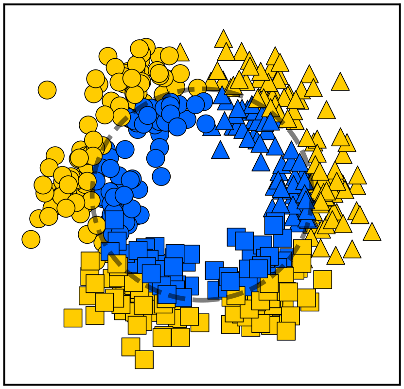
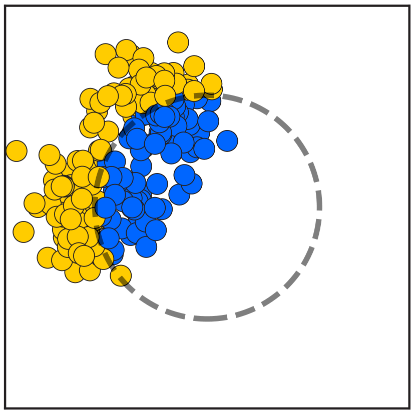
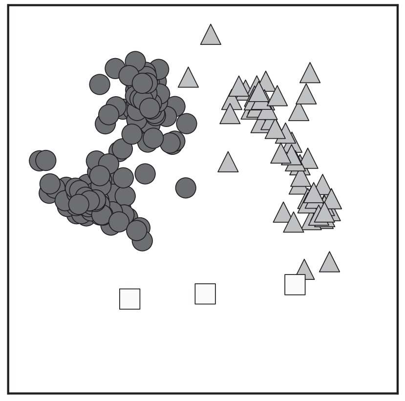
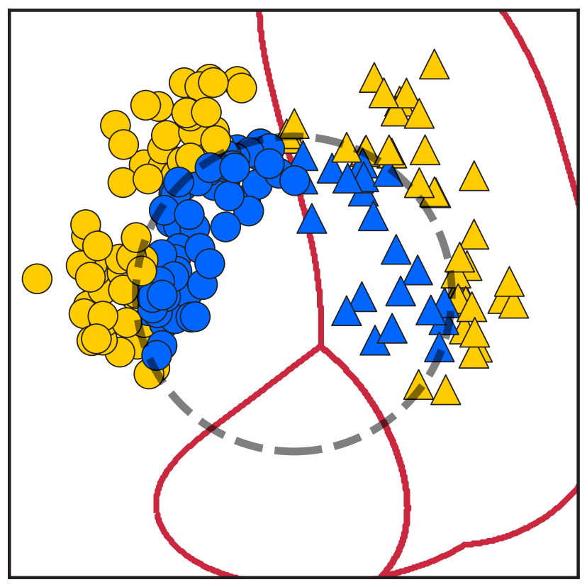
Fig. 3(a) shows the problem setting. Circle, triangle, and square points are different local datasets from each provider. Each dataset is drawn from a mixture of two Gaussians. The means of these Gaussians are arranged around a circle denoted by the grey dashed line. Points inside the grey circle are labeled as blue class, and points outside the circle are labeled as yellow class, thus the binary classification problem. We should emphasize that their local datasets are unobservable to others, they are plotted in the same figure just for space-saving. RBF kernel SVMs are used as pre-trained models.
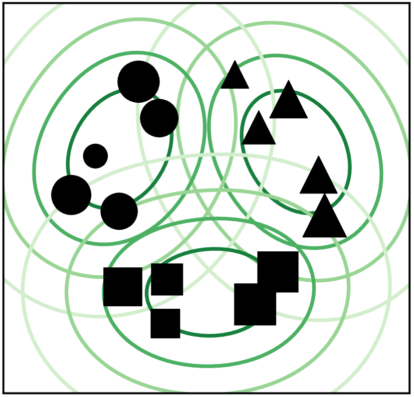
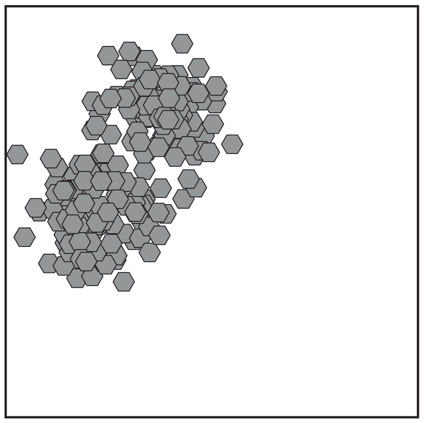
The results of reduced set construction by running Algorithm 1 are shown in Fig. 3(b). We set here, which is enough for approximating the empirical KME in this example. Different from the original empirical KME , where all points contribute equally to the embedding, the constructed reduced KME introduced more freedom by using variable weights . In the figure, we use the size of markers to illustrate the value of weights. These reduced sets implicitly “remember” the Gaussian mixtures behind local datasets and serve as specifications to tell future users where each pre-trained model works well.
In the deployment phase, we evaluate both task-recurrent and instance-recurrent assumptions. In Fig. 4, we draw test points from the same distribution of the “circle” dataset. As expected, our method successfully finds the match and predict all the data by the pre-trained “circle” model.
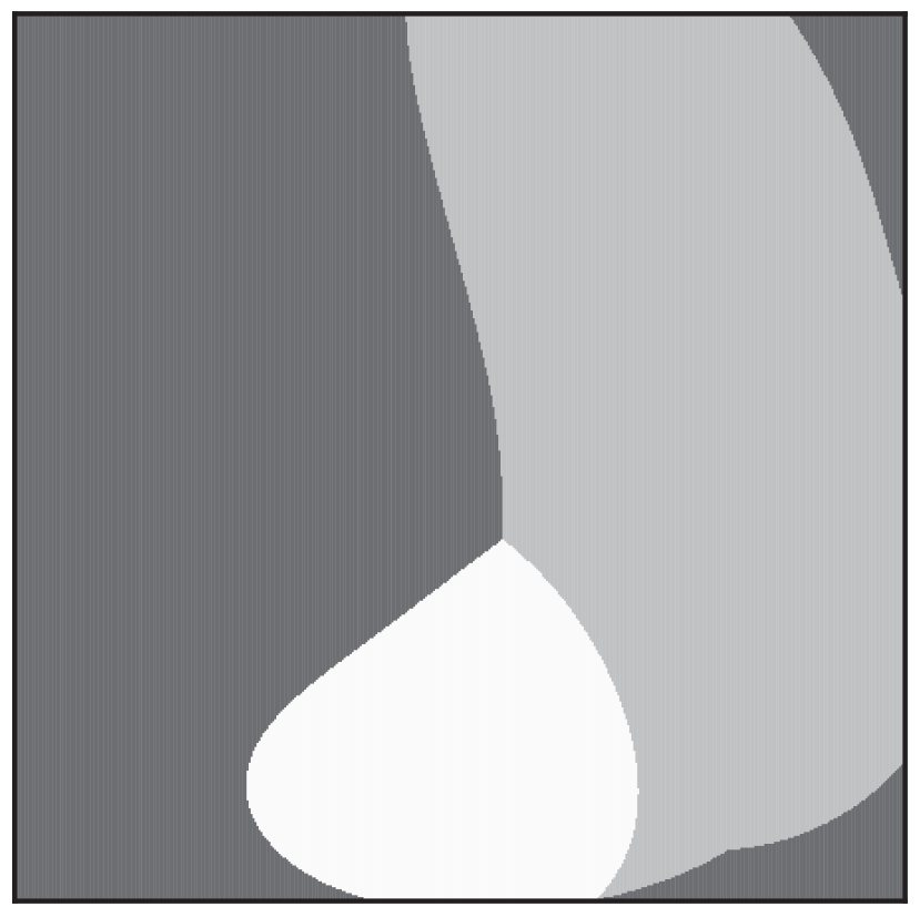
In instance-recurrent setting, we set the mixture weight of (circle, triangle, square) to and test our method. Our estimated mixture weight is , closing to the groundtruth. Given the accurately estimated mixture weight, we are able to generate a mimicked sample by kernel herding. It is clear in Fig 5(b) that the drawn distribution is similar to the testing data and with assigned labels. The weight of square is low but not zero, therefore there are still few squares in the sample set. The learned selector divides the feature space into three regions, and all the testing points fall into the “circle” or “triangle” region. Predictions in Fig. 5(d) achieves accuracy 92.5%, and errors are mainly made from pre-trained models themselves, not from the selection of ours.

The toy example gives a visual demonstration of our two-phase framework. We can see from this example that the inaccessibility of private training data and reusability of pre-trained models are met. In the next section, we post results on two benchmark datasets.
6.2 Benchmark
In this section, we evaluate our proposal on two widely used benchmark datasets: image dataset CIFAR-100 [Krizhevsky, 2009] and text dataset 20-newsgroup [Joachims, 1997].
CIFAR-100 has 100 classes and they are grouped into 20 superclasses, and each superclass contains 5 classes. For example, the superclass “flower” includes {orchid, poppy, rose, sunflower, tulip}. It is natural to use this dataset to simulate our setting. We divide CIFAR-100 into 20 local datasets, each having images from one superclass, and build 5-class local neural network classifiers on them.
20-newsgroup is a popular text classification benchmark and it has similar hierarchical structure as CIFAR-100. There are 5 superclasses {comp, rec, sci, talk, misc} and each is considered a local dataset for training local models in the upload phase.
Kernel methods usually cannot work directly on the raw-pixel level or raw-document level, therefore we use off-the-shelf deep models to extract meaningful feature vectors. For CIFAR-100, features are the outputs from the penultimate layer of ResNet-110.111Trained by running the command of ResNet-110 in https://github.com/bearpaw/pytorch-classification/blob/master/TRAINING.md For 20-newsgroup, an LSTM is built on GloVe [Pennington et al., 2014] word embeddings, and features are extracted from the global max-pooling layer. These feature vectors are used for RKME construction in the upload phase. Gaussian kernel as defined in (2) with is used in both datasets, and the size of the reduced set is set to , which is a tiny ratio of the original datasets.
We compare our method with a naive baseline MAX and a related method HMR [Wu et al., 2019]. MAX simply uses all the pre-trained models to predict one test instance, and takes out the most confident predicted class. HMR incorporates a communication protocol which exchanges several selected key examples to update models, and then does predictions like MAX. In this comparison we allow HMR to exchange up to 1000 examples. All three methods use the same pool of pre-trained models. Instance-recurrent setting is simulated by randomly mixing testing data from different number of solved tasks. The mean accuracy of 10 times each setting are reported in Table 1&2, and the last row reports the non-private accuracy of a global model trained on merged data.
| Task-recurrent | Instance-recurrent | ||||
| #Mixing tasks | 1 | 2 | 5 | 10 | 20 |
| MAX | 43.00 | 42.10 | 41.51 | 41.62 | 41.44 |
| HMR | 70.58 | 68.91 | 68.93 | 68.88 | 68.81 |
| Ours | 86.22 | 72.91 | 72.57 | 71.07 | 68.79 |
| Global | 75.08 | 73.24 | 73.31 | 71.86 | 73.24 |
| Task-recurrent | Instance-recurrent | ||||
| #Mixing tasks | 1 | 2 | 3 | 4 | 5 |
| MAX | 58.65 | 55.76 | 53.03 | 51.94 | 50.68 |
| HMR | 72.01 | 72.19 | 70.86 | 70.53 | 70.09 |
| Ours | 83.13 | 76.03 | 75.10 | 74.02 | 72.68 |
| Global | 72.06 | 73.24 | 73.31 | 71.86 | 73.24 |
It is clear that our method performs best with a large margin in the task-recurrent setting. Other methods cannot exploit the prior knowledge that the current task is identical to one of the solved tasks, while our minimum-MMD measure can successfully find out the fittest pre-trained model.
In the instance-recurrent setting, ours is the best in most cases. We are even better than the non-private global model in the 20-newsgroup dataset. It is possible because the global model is an ERM optimizer on the merged data, which is the best model for i.i.d testing examples but not adaptive to a changed unknown distribution. While ours can estimate the mixing weight and adapt to a different biased test distribution in the deployment phase. Ours is increasingly better when the number of mixing tasks goes smaller, because we can preclude some impossible output classes by selecting right pre-trained models.
Besides, we should keep in mind that the comparison is unfair because HMR and global are not fully privacy-preserving methods. Our proposal gets better or competitive performance without exposing any raw data points.
6.3 Real-World Project
Communication quality is the key to user experience for a telecommunications company. We participated in an industrial project called crystal-voice at Huawei Technologies Co., Ltd. Huawei tested a novel technology “deep cover” on base stations to improve the quality. But engineers observed the gain of quality varies because of differences about user behaviors and environments among stations. They want to predict how much can we gain in a new base station, to decide whether it is profitable to deploy “deep cover” on it.
Every user covered by a base station is represented by a feature vector, and a real-valued quality gain. It is strictly forbidden to move users’ information out of stations, but each station has enough data to build a strong local model and share it in a pool. Therefore, our proposal is a wise choice to handle this problem.
In the upload phase, a local ridge regression model is trained in each base station. We then construct RKME (set size , Gaussian kernel ) as the specification, and upload the models and specifications into a learnware pool. All the vectors in the specification are constructed “pseudo” users, protecting the raw information from thousands of users.
In the deployment phase, we run instance-recurrent procedure on a new base station. There are 8 anonymous base stations in total, therefore we test our method 8 times. At each time, we select one of them as the current task and the rest 7 as solved tasks.
Four methods are compared with ours. Two model reuse baselines RAND/AVG and two transfer learning methods KMM [Huang et al., 2006]/mSDA [Chen et al., 2012]. RAND means randomly selecting one pre-trained model from other base stations to predict each user’s gain. AVG means averaging the outputs of all regressors in the model pool as predictions. KMM reweights source data to train a better model for the testing data. mSDA learns robust feature representations over all domains.
We should notice that the model reuse methods are private, but transfer learning methods are non-private because they need to see both testing and training data in the deployment phase. The mean results are reported in Table 3. MAX and HMR in Section 6.2 cannot be used for this regression task, while our framework is agnostic to the task and type of pre-trained models.
| RMSE | 3p30 | 5p30 | 3f1 | ||
|---|---|---|---|---|---|
| Model reuse | RAND | .0363 | .3730 | .4412 | .7320 |
| AVG | .0326 | .4272 | .4535 | .7712 | |
| Ours | .0279 | .5281 | .5205 | .8082 | |
| Transfer | KMM | .0291 | .5018 | .5222 | .7911 |
| mSDA | .0285 | .5105 | .5324 | .8034 |
Our method not only outperforms model reuse baselines in terms of root-mean-square error (RMSE), but is also superior on the other measurements required in the real business. “3p30” is the ratio of users whose gain value is above 3% and the prediction error is lower than 30%. “5p30” is defined similarly. “3f1” is the F1-measure if we consider the users whose gain value above 3% are positive class. Our method is even better than mSDA and KMM in some measurements. Considering these two transfer learning methods break the privacy, ours sacrifice a little performance in “5p30” while keeping the data safe in base stations.
7 Conclusion
In this paper, we propose reduced kernel mean embedding as the specification in the learnware paradigm, and implement a two-phase pipeline based on it. RKME is shown to protect raw training data in the upload phase and can identify reusable pre-trained models in the deployment phase. Experimental results, including a real industrial project at Huawei, validate the effectiveness of it. This is the first valid specification with practical success to our best knowledge.
In the future, we plan to incorporate more powerful kernel methods to directly measure the similarity in the raw high-dimensional feature space when constructing RKME. It remains an open challenge to design other types of valid specifications, under assumptions which are even weaker than the instance-recurrent assumption.
References
- Arif and Vela [2009] O. Arif and P. A. Vela. Kernel map compression using generalized radial basis functions. In IEEE 12th International Conference on Computer Vision, pages 1119–1124, 2009.
- Balog et al. [2018] M. Balog, I. O. Tolstikhin, and B. Schölkopf. Differentially private database release via kernel mean embeddings. In Proceedings of the 35th International Conference on Machine Learning, pages 423–431, 2018.
- Burges [1996] C. J. C. Burges. Simplified support vector decision rules. In Proceedings of the 13th International Conference on Machine Learning, pages 71–77, 1996.
- Chen et al. [2012] M. Chen, Z. E. Xu, K. Q. Weinberger, and F. Sha. Marginalized denoising autoencoders for domain adaptation. In Proceedings of the 29th International Conference on Machine Learning, 2012.
- Chen [2013] Y. Chen. Herding: Driving Deterministic Dynamics to Learn and Sample Probabilistic Models DISSERTATION. PhD thesis, University of California, Irvine, 2013.
- Chen et al. [2010] Y. Chen, M. Welling, and A. J. Smola. Super-samples from kernel herding. In Proceedings of the 26th Conference on Uncertainty in Artificial Intelligence, pages 109–116, 2010.
- Clyburne-Sherin et al. [2019] A. Clyburne-Sherin, X. Fei, and S. A. Green. Computational reproducibility via containers in social psychology. Meta-Psychology, 3, 2019.
- Doran et al. [2014] G. Doran, K. Muandet, K. Zhang, and B. Schölkopf. A permutation-based kernel conditional independence test. In Proceedings of the 30th Conference on Uncertainty in Artificial Intelligence, pages 132–141, 2014.
- Du et al. [2017] S. S. Du, J. Koushik, A. Singh, and B. Póczos. Hypothesis transfer learning via transformation functions. In Advances in Neural Information Processing Systems, pages 574–584, 2017.
- Duan et al. [2009] L. Duan, I. W. Tsang, D. Xu, and T.-S. Chua. Domain adaptation from multiple sources via auxiliary classifiers. In Proceedings of the 26th International Conference on Machine Learning, pages 289–296, 2009.
- Fukumizu et al. [2007] K. Fukumizu, A. Gretton, X. Sun, and B. Schölkopf. Kernel measures of conditional dependence. In Advances in Neural Information Processing Systems, pages 489–496, 2007.
- Gretton et al. [2012] A. Gretton, K. M. Borgwardt, M. J. Rasch, B. Schölkopf, and A. Smola. A kernel two-sample test. Journal of Machine Learning Research, 13(Mar):723–773, 2012.
- Hard et al. [2018] A. Hard, K. Rao, R. Mathews, F. Beaufays, S. Augenstein, H. Eichner, C. Kiddon, and D. Ramage. Federated learning for mobile keyboard prediction. arXiv preprint arXiv:1811.03604, 2018.
- Hinton et al. [2014] G. E. Hinton, O. Vinyals, and J. Dean. Distilling the knowledge in a neural network. In NIPS Workshop on Deep Learning and Representation Learning, 2014.
- Hoffman et al. [2018] J. Hoffman, M. Mohri, and N. Zhang. Algorithms and theory for multiple-source adaptation. In Advances in Neural Information Processing Systems, pages 8256–8266, 2018.
- Huang et al. [2006] J. Huang, A. J. Smola, A. Gretton, K. M. Borgwardt, and B. Schölkopf. Correcting sample selection bias by unlabeled data. In Advances in Neural Information Processing Systems, pages 601–608, 2006.
- Jitkrittum et al. [2016] W. Jitkrittum, Z. Szabó, K. P. Chwialkowski, and A. Gretton. Interpretable distribution features with maximum testing power. In Advances in Neural Information Processing Systems, pages 181–189, 2016.
- Joachims [1997] T. Joachims. A probabilistic analysis of the rocchio algorithm with TFIDF for text categorization. In Proceedings of the 14th International Conference on Machine Learning, pages 143–151, 1997.
- Konečný et al. [2016] J. Konečný, H. B. McMahan, F. X. Yu, P. Richtarik, A. T. Suresh, and D. Bacon. Federated learning: Strategies for improving communication efficiency. In NIPS Workshop on Private Multi-Party Machine Learning, 2016.
- Krizhevsky [2009] A. Krizhevsky. Learning multiple layers of features from tiny images. Technical report, 2009.
- Kuzborskij and Orabona [2013] I. Kuzborskij and F. Orabona. Stability and hypothesis transfer learning. In Proceedings of the 30th International Conference on Machine Learning, pages 942–950, 2013.
- Lopez-Paz et al. [2015] D. Lopez-Paz, K. Muandet, B. Schölkopf, and I. O. Tolstikhin. Towards a learning theory of cause-effect inference. In Proceedings of the 32nd International Conference on Machine Learning, pages 1452–1461, 2015.
- Mansour et al. [2008] Y. Mansour, M. Mohri, and A. Rostamizadeh. Domain adaptation with multiple sources. In Advances in Neural Information Processing Systems, pages 1041–1048, 2008.
- Mansour et al. [2009] Y. Mansour, M. Mohri, and A. Rostamizadeh. Multiple source adaptation and the rényi divergence. In Proceedings of the 25th Conference on Uncertainty in Artificial Intelligence, pages 367–374, 2009.
- Muandet and Schölkopf [2013] K. Muandet and B. Schölkopf. One-class support measure machines for group anomaly detection. In Proceedings of the 29th Conference on Uncertainty in Artificial Intelligence, pages 449––458, 2013.
- Muandet et al. [2017] K. Muandet, K. Fukumizu, B. K. Sriperumbudur, and B. Schölkopf. Kernel mean embedding of distributions: A review and beyond. Foundations and Trends in Machine Learning, 10(1-2):1–141, 2017.
- Pathak et al. [2010] M. A. Pathak, S. Rane, and B. Raj. Multiparty differential privacy via aggregation of locally trained classifiers. In Advances in Neural Information Processing Systems, pages 1876–1884, 2010.
- Pennington et al. [2014] J. Pennington, R. Socher, and C. D. Manning. Glove: Global vectors for word representation. In Proceedings of the 2014 Conference on Empirical Methods in Natural Language Processing, pages 1532–1543, 2014.
- Schölkopf and Smola [2002] B. Schölkopf and A. J. Smola. Learning with Kernels: support vector machines, regularization, optimization, and beyond. MIT Press, 2002.
- Schölkopf et al. [1999] B. Schölkopf, S. Mika, C. J. C. Burges, P. Knirsch, K. Müller, G. Rätsch, and A. J. Smola. Input space versus feature space in kernel-based methods. IEEE Transactions on Neural Networks, 10(5):1000–1017, 1999.
- Smola et al. [2007] A. J. Smola, A. Gretton, L. Song, and B. Schölkopf. A Hilbert space embedding for distributions. In ALT, pages 13–31, 2007.
- Sun et al. [2015] S. Sun, H. Shi, and Y. Wu. A survey of multi-source domain adaptation. Information Fusion, 24:84–92, 2015.
- Tommasi et al. [2014] T. Tommasi, F. Orabona, and B. Caputo. Learning categories from few examples with multi model knowledge transfer. IEEE Transactions on Pattern Analysis and Machine Intelligence, 36(5):928–941, 2014.
- Welling [2009] M. Welling. Herding dynamic weights for partially observed random field models. In Proceedings of the 25th Conference on Uncertainty in Artificial Intelligence, pages 599–606, 2009.
- Wu et al. [2019] X.-Z. Wu, S. Liu, and Z.-H. Zhou. Heterogeneous model reuse via optimizing multiparty multiclass margin. In Proceedings of the 36th International Conference on Machine Learning, pages 6840–6849, 2019.
- Yang et al. [2019] Q. Yang, Y. Liu, T. Chen, and Y. Tong. Federated machine learning: Concept and applications. ACM Transactions on Intelligent Systems and Technology, 10(2):12, 2019.
- Zhou [2016] Z.-H. Zhou. Learnware: on the future of machine learning. Frontiers of Computer Science, 10(4):589–590, 2016.
- Zhou and Jiang [2004] Z.-H. Zhou and Y. Jiang. Nec4.5: Neural ensemble based C4.5. IEEE Transactions on Knowledge and Data Engineering, 16(6):770–773, 2004.