High-Quality Hierarchical Process Mapping

Abstract

Partitioning graphs into blocks of roughly equal size such that few edges run between blocks is a frequently needed operation when processing graphs on a parallel computer. When a topology of a distributed system is known an important task is then to map the blocks of the partition onto the processors such that the overall communication cost is reduced. We present novel multilevel algorithms that integrate graph partitioning and process mapping. Important ingredients of our algorithm include fast label propagation, more localized local search, initial partitioning, as well as a compressed data structure to compute processor distances without storing a distance matrix. Experiments indicate that our algorithms speed up the overall mapping process and, due to the integrated multilevel approach, also find much better solutions in practice. For example, one configuration of our algorithm yields better solutions than the previous state-of-the-art in terms of mapping quality while being a factor 62 faster. Compared to the currently fastest iterated multilevel mapping algorithm Scotch, we obtain 16% better solutions while investing slightly more running time.

1 Introduction

The performance of applications that run on high-performance computing systems depends on many factors such as the capability and topology (structure) of the underlying communication system, the required communication (patterns, frequencies, volumes, and dependencies) between processes in the given applications, and the software and algorithms used to realize the communication. For example, communication is typically faster (has lower latency, higher bandwidth, more communication channels) if communicating processes are located on the same physical processor node compared to cases where processes reside on different nodes. This becomes even more pronounced for large supercomputer systems where processors are hierarchically organized (e. g., islands, racks, nodes, processors, cores) with corresponding communication links of similar quality, and where differences in the process placement can have a huge impact on the communication performance (latency, bandwidth, congestion). Often the communication pattern between application processes is or can be known. Additionally, a hardware topology description that reflects the capacity of the communication links is typically available. Hence, it is natural to attempt to find a good mapping of the application processes onto the hardware processors such that pairs of processes that frequently communicate large amounts of data are located closely. Finding such best or just good mappings is the objective of some usually hard optimization problems.

Previous work can be grouped into two categories. One line of research intertwines process mapping with multilevel graph partitioning (see for example [51, 33]). To this end, the objective of the partitioning algorithm – most commonly the number of cut edges – is typically replaced by an objective function that considers the processor distances. Throughout these algorithms, the distances are directly taken into consideration. The second category decouples partitioning and mapping (see for example [43, 8, 19, 31]). First, a graph partitioning algorithm is used to partition a large graph into $k$ blocks, while minimizing some measure of communication, such as edge-cut, and at the same time balancing the load (size of the blocks). Afterwards, a coarser model of computation and communication is created in which the number of nodes matches the number of processing elements (PEs) in the given processor network. This model is then mapped to a processor network of $k$ PEs with given pair-wise distances using a process mapping algorithm. As shown in [5], the decoupling approach can lead to worse results than the integrated approach. We refer the reader to [6, 9] for more details on mapping and graph partitioning.

The starting point for this research is as follows. Recently, process mapping algorithms have made two assumptions that are typically valid for modern supercomputers and the applications that run on those: communication patterns are sparse and there is a hierarchical communication topology where links on the same level in the hierarchy exhibit the same communication speed. Using these assumptions, better decoupled – non-integrated – mapping algorithms have been obtained, e.g. [43]. In this problem formulation, the model of computation and communication is first partitioned using a standard graph partitioning algorithm, and then a smaller model that has the same number of nodes as the underlying network of processors is mapped. On the other hand, there has been a large body of work on the multilevel (hyper-)graph partitioning problem, which led to enhanced partitioning quality or faster local search [37, 38, 27, 41, 40]. The multilevel approach [9] is probably the most prominently used algorithm in the graph partitioning field. Here, the input is recursively contracted to obtain a smaller instance which should reflect the same basic structure as the input. After applying an initial partitioning algorithm to the smallest instance, contraction is undone and, at each level, local search methods are used to improve the partitioning induced by the coarser level. Recent enhancements to the multilevel scheme include novel local search techniques such as very localized local search algorithms, fast label propagation algorithms, or gain caches to avoid expensive recomputations throughout local search algorithms.

Our main contribution in this paper is the integration of process mapping into a multilevel scheme with high-quality local search techniques and recently developed non-integrated mapping algorithms. Additionally, we introduce faster techniques that avoid to store distance matrices. Overall, our algorithms are able to compute better solutions than other recent heuristics for the problem scale well to large instances. The rest of this paper is organized as follows. In Section 2, we introduce basic concepts and describe relevant related work in more detail. We present our main contributions in Section 3. We implemented the techniques presented here in the graph partitioning framework KaHIP [38] (Karlsruhe High Quality Graph Partitioning). We present a summary of extensive experiments to evaluate algorithm performance in Section 4. The experiments indicate that our new integrated algorithm improves mapping quality over other state-of-the-art integrated and non-integrated mapping algorithms. For example, one configuration of our algorithm yields better solutions than the previous state-of-the-art in terms of mapping quality while being a factor 62 faster. Compared to the currently fastest iterated multilevel mapping algorithm Scotch, we obtain 16% better solutions while investing slightly more running time. Most importantly, hierarchical multisection algorithms that take the system hierarchy into account for model creation improve the results of the overall process mapping significantly.

2 Preliminaries

The communication requirements between the components of a set of processes in (some section of) an application can be represented by a weighted communication graph. The underlying hardware topology can likewise be represented by a weighted graph, particularly a complete graph since any two physical processors can communicate with each other facilitated by the routing system. This complete graph can be represented by a topology cost matrix reflecting the costs of routing along shortest or cheapest paths between physical processors. Furthermore, it does not need to be explicitly expressed if the topology is organized as a regular hierarchy of components with fixed communication cost per message inside each level. We tackle the problem of embedding a communication graph onto a topology graph under optimization criteria that we explain below. Unless otherwise mentioned, a processing element (PE) represents a core of a machine.

2.1 Basic Concepts

Let $G=(V=\{0,\ldots,n-1\},E)$ be an undirected graph with edge weights $\omega:E\to\mathbb{R}_{>0}$, vertex weights $c:V\to\mathbb{R}_{\geq 0}$, $n=|V|$, and $m=|E|$. We generalize $c$ and $\omega$ functions to sets, such that $c(V^{\prime})=\sum_{v\in V^{\prime}}c(v)$ and $\omega(E^{\prime})=\sum_{e\in E^{\prime}}\omega(e)$. Let $N(v)=\left\{u\,:\,\left\{v,u\right\}\in E\right\}$ denote the neighbors of a vertex $v$. Let $I(v)$ denote the set of edges incident to $v$. A graph $S=(V^{\prime},E^{\prime})$ is said to be a subgraph of $G=(V,E)$ if $V^{\prime}\subseteq V$ and $E^{\prime}\subseteq E\cap(V^{\prime}\times V^{\prime})$. When $E^{\prime}=E\cap(V^{\prime}\times V^{\prime})$, $S$ is an induced subgraph.

The graph partitioning problem (GPP) consists of assigning each node of $G$ to exactly one of $k$ distinct blocks respecting a balancing constraint in order to minimize the edge-cut. More precisely, GPP partitions $V$ into $k$ blocks $V_{1}$,…,$V_{k}$ (i. e., $V_{1}\cup\cdots\cup V_{k}=V$ and $V_{i}\cap V_{j}=\emptyset$ for $i\neq j$), which is called a $k$-partition of $G$. The balancing constraint demands that the sum of node weights in each block does not exceed a threshold associated with some allowed imbalance $\epsilon$. More specifically, $\forall i\leavevmode\nobreak\ \in\leavevmode\nobreak\ \{1,\ldots,k\}:$ $c(V_{i})\leq L_{\max}:=\big{\lceil}(1+\epsilon)\frac{c(V)}{k}\big{\rceil}$. Let a block $V_{i}$ be called $\lambda$-underloaded if $|V_{i}|+\lambda\leq L_{\max}$ and overloaded if $|V_{i}|>L_{\max}$. The edge-cut of a $k$-partition consists of the total weight of the edges crossing blocks, i. e., $\sum_{i<j}\omega(E_{ij})$, where $E_{ij}:=\left\{\left\{u,v\right\}\in E\,:\,u\in V_{i},v\in V_{j}\right\}$. An abstract view of the partitioned graph is a quotient graph $\mathcal{Q}$, in which nodes represent blocks and edges are induced by the connectivity between blocks. More precisely, there is an edge in the quotient graph if there is an edge that runs between the blocks in the original, partitioned graph. We call neighboring blocks a pair of blocks connected to each other by an edge in the quotient graph. If a node $v\in V_{i}$ has a neighbor $w\in V_{j},i\neq j$, then it is called a boundary node. Let $R(v)$ be the set of all blocks containing at least one element from $\{v\}\cup N(v)$.

Assume that we have $n$ processes and a topology containing $k$ PEs. Let $\mathcal{C}\in\mathbb{R}^{n\times n}$ denote the communication matrix and let $\mathcal{D}\in\mathbb{R}^{k\times k}$ denote the (implicit) topology matrix or distance matrix. In particular, $\mathcal{C}_{i,j}$ represents the required amount of communication between processes $i$ and $j$, while $\mathcal{D}_{x,y}$ represents the cost of each communication between PEs $x$ and $y$. Hence, if processes $i$ and $j$ are respectively assigned to PEs $x$ and $y$, or vice-versa, the communication cost between $i$ and $j$ will be $\mathcal{C}_{i,j}\mathcal{D}_{x,y}$. Throughout this work, we assume that $\mathcal{C}$ and $\mathcal{D}$ are symmetric – otherwise one can create equivalent problems with symmetric inputs [8].

In this work, we deal with topologies organized as homogeneous hierarchies, even though our algorithms could be extended to heterogeneous hierarchies in a straightforward way. Let $\mathcal{S}=a_{1}:a_{2}:...:a_{\ell}$ be a sequence describing the hierarchy of a supercomputer. The sequence should be interpreted as each processor having $a_{1}$ cores, each node $a_{2}$ processors, each rack $a_{3}$ nodes, and so forth, such that the total number of processors is $k=\Pi_{i=1}^{\ell}a_{i}$. Let $D=d_{1}:d_{2}:\ldots:d_{\ell}$ be a sequence describing the communication cost inside each hierarchy level, meaning that two cores in the same processor communicate with cost $d_{1}$, two cores in the same node but in different processors communicate with cost $d_{2}$, two cores in the same rack but in different nodes communicate with cost $d_{3}$, and so forth.

Throughout the paper, we assume that the input communication matrix is already given as a graph $G_{\mathcal{C}}$, i. e., no conversion of the matrix into a graph is necessary. More precisely, the graph representation is defined as $G_{\mathcal{C}}:=(\{1,\ldots,n\},E[\mathcal{C}])$ where $E[\mathcal{C}]:=\{(u,v)\mid\mathcal{C}_{u,v}\not=0\}$. In other words, $E[\mathcal{C}]$ is the edge set of the processes that need to communicate with each other. Note that the set contains forward and backward edges, and that the weight of each edge in the graph equals the corresponding entry in the communication matrix $\mathcal{C}$.

Our main focus in this work is the general process mapping problem (GPMP). It consists of assigning each node of a given communication graph to a specific PE in a communication topology while respecting a balancing constraint (the same as in the graph partitioning problem above) in order to minimize the total communication costs. Within the scope of this work, the number of nodes (processes) $n$ in the communication graph is much larger than the number of PEs $k$ in the topology graph which matches most real-world situations. Let the mapping function that maps a node onto its block be $\Pi:\{1,\ldots,n\}\mapsto\{1,\ldots,k\}$. Hence, the objective function of GPMP is to minimize $J(\mathcal{C},\mathcal{D},\Pi):=\sum_{i,j}\mathcal{C}_{i,j}\mathcal{D}_{\Pi(i),\Pi(j)}$. Many authors deal with the specific case in which $n=k$, resulting in the one-to-one process mapping problem (OPMP), where each process $i$ is assigned to a unique PE $\Pi(i)$. Within the context of OPMP, searching for the inverse permutation instead, i. e., assigning PE $x$ to node $\Pi^{-1}(x)$, results in the same problem since $\Pi$ is a bijection.

GPP and OPMP are both NP-hard problems [14, 35]. Since GPP and OPMP are special cases of GPMP, the latter is also NP-hard. Hence, exact efficient algorithms to solve GPMP are very unlikely, which justifies the use of heuristics to obtain reasonably good solutions for real-world instances within a reasonable time. Two of the most common methods to solve GPMP are the two-phase approach and the integrated approach. In the two-phase approach, GPMP is solved in two consecutive steps: (i) a heuristic for GPP is applied in the communication graph, obtaining a balanced $k$-partition; (ii) a heuristic for OPMP is used to map the blocks of the $k$-partition onto the topology of PEs. On the other hand, the integrated approach consists of tackling GPMP directly, i. e., not decomposing the input problem into $k$ independent sub-problems first.

2.2 Multilevel Approach

In this section, we characterize the multilevel approach within the scope of GPMP, although the same basic structure is extensible to many other problems, such as GPP. Before describing the multilevel scheme, we need to define the terms contraction and uncontraction. Contracting an edge $e=\left\{u,v\right\}$ consists of replacing the nodes $u$ and $v$ by a new node $x$ connected to the former neighbors of $u$ and $v$. We set $c(x)=c(u)+c(v)$ so that the weight of a node at each level is the sum of weights of the contracted nodes. If replacing edges of the form $\left\{u,w\right\}$, $\left\{v,w\right\}$ would generate two parallel edges $\left\{x,w\right\}$, a single edge with $\omega(\left\{x,w\right\})=\omega(\left\{u,w\right\})+\omega(\left\{v,w\right\})$ is inserted. The uncontraction of a node consists of undoing the contraction that gave rise to it. In order to avoid tedious notation, $G$ will denote the current state of the graph, either before or after (un)contraction, unless we explicitly want to refer to different states of the graph.

A multilevel approach to solve GPMP consists of three main phases. In the contraction (coarsening) phase, successive approximations of an original input graph are created. In particular, the first-level approximation is obtained directly through a contraction on the original graph, the second-level approximation is obtained through a contraction on the first-level approximation, and so forth. Hence, each of these approximations conserves structural information about the input graph, but in different levels: from micro-structural (particular) information in the finest approximation to macro-structural (general) information in the coarsest approximation. The contractions quickly reduce the size of the graph and stop as soon as it becomes sufficiently small to be partitioned and mapped by an expensive algorithm. In the construction phase, an initial mapping is produced for the coarsest approximation of the input graph. Due to the way we define contraction, every mapping of the coarsest level implies a corresponding mapping of the input graph with equal objective function and balance. In the local improvement (or uncoarsening) phase, we uncontract previously contracted nodes to go back through each level, from the coarsest approximation to the original graph. After each uncoarsening, local improvement algorithms move nodes between blocks in order to improve the objective function or balance.

2.3 Related Work

There has been an immense amount of research on GPP, and the reader is referred to [6, 9, 42] for extensive material and references. The most successful general-purpose methods to solve GPP for huge real-world graphs are based on the multilevel approach. The basic idea of this approach can be traced back to multigrid solvers for systems of linear equations [45], and its first application to GPP was by Barnard and Simon [4]. The most commonly used formulation of the multilevel scheme was proposed by Hendrickson and Leland [20]. Similar multilevel schemes are used for other graph partitioning problem formulations such as DAG partitioning[30, 21, 29], hypergraph partitioning [24, 2], graph clustering [7, 11], graph drawing [49, 28] or the node separator problem [39, 17]. Among the most successful multilevel software packages to solve GPP, we mention Jostle [50], Metis [23], Scotch [32], and KaHIP [36].

Systems like KaHIP [36] and Metis [23] typically compute a $k$-partition on the coarsest level through a recursive bisection strategy or a direct $k$-way partitioning scheme. In recursive bisection, the graph is recursively divided into two blocks until the number of blocks is reached, i. e., a bisection algorithm is used to split the graph into two blocks. More precisely, each bisection step itself uses a multilevel algorithm that stops as soon as the number of nodes is below a small threshold. To obtain a bipartition in the coarsest level, KaHIP uses the greedy graph growing algorithm. In KaHIP, if $k$ is not even, the graph gets split into two blocks, $V_{1}$ and $V_{2}$, such that $c(V_{1})\leq\big{\lfloor}\frac{k}{2}\big{\rfloor}L_{\max}$, $c(V_{2})\leq\big{\lceil}\frac{k}{2}\big{\rceil}L_{\max}$. Block $V_{1}$ will be recursively partitioned in $\lfloor\frac{p}{2}\rfloor$ blocks and block $V_{2}$ will be recursively partitioned in $\lceil\frac{p}{2}\rceil$ blocks.

In addition to GPP, Jostle and Scotch can also solve GPMP. Jostle integrates local search into a multilevel scheme to partition the model of computation and communication. In this scheme, it solves the problem on the coarsest level and afterwards performs refinements based on the user-supplied network communication model. On the other hand, Scotch performs dual recursive bipartitioning to compute a mapping. More precisely, it starts the recursion considering all given processes and PEs. At each recursion level, it bipartitions the communication graph and also the distance graph with a graph bipartitioning algorithm. The first (resp., second) block of the communication graph is then assigned to the first (resp., second) block of the distance graph. The recursion proceeds until the distance graph only contains one vertex.

There is likewise a large literature on OPMP, often in the context of scientific applications using the Message Passing Interface (MPI). Hatazaki [18] was among the first authors to propose graph partitioning to solve the MPI process mapping of a virtual unweighted topology onto a hardware topology organized in modules and sub-modules. Träff [46] used a similar approach to implement one of the first non-trivial mappings designed for the NEC SX-series of parallel vector computers. Mercier and Clet-Ortega [25] and later Mercier and Jeannot [26] simplified the mapping problem to ignore the whole network topology except that inside each node. They also investigated multiple placement policies to enhance overall system performance. Yu et al. [52] discussed and implemented graph embedding heuristics for the BlueGene $3d$ torus systems. Hoefler and Snir [22] optimized instead the congestion of the mapping, additionally providing a proof that this problem is NP-complete, a heuristic to solve it, and an experimental evaluation based on application data from the Florida Sparse Matrix Collection. Routing-aware mapping heuristics taking the hierarchy of specific hardware topologies into account were discussed in [1]. Vogelstein et al. [47] concentrated on solving OPMP. They proposed a gradient–based heuristic that involves solving assignment problems and gave experimental evidence for better solution quality and speed compared to other heuristics.

Müller-Merbach [31] proposed a greedy construction method to obtain an initial permutation for OPMP. The method roughly works as follows: Initially compute the total communication volume for each process and also the sum of distances from each core to all the others. Note that this corresponds to the weighted degrees of the nodes in the communication and distance models, respectively. Afterwards, the process with the largest communication volume is assigned to the core with the smallest total distance. To build a complete assignment, the algorithm proceeds by looking at unassigned processes and cores. For each of the unassigned processes, the communication load to already assigned vertices is computed. For each core, the total distance to already assigned cores is computed. The process with the largest communication sum is assigned to the core with the smallest distance sum. Glantz et al. [15] noted that the algorithm does not link the choices for the vertices and cores and hence propose a modification of this algorithm called GreedyAllC (the best algorithm in [15]). GreedyAllC links the mapping choices by scaling the distance with the amount of communication to be done. The algorithm has the same asymptotic complexity and memory requirements as the algorithm by Müller-Merbach.

Heider [19] proposed a method to improve an already given solution for OPMP. The method repeatedly tries to perform swaps in the assignment. To do so, the author defines a pair-exchange neighborhood $N(\Pi)$ that contains all permutations that can be reached by swapping two elements in $\Pi$. Here, swapping two elements means that $\Pi^{-1}(i)$ will be assigned to processor $j$ and $\Pi^{-1}(j)$ will be assigned to processor $i$ after the swap is done. The algorithm then looks at the neighborhood in a cyclic manner. More precisely, in each step the current pair $(i,j)$ is updated to $(i,j+1)$ if $j<n$, to $(i+1,i+2)$ if $j=n$ and $i<n-1$, and lastly to $(1,2)$ if $j=n$ and $i=n-1$. A swap is performed if it yields a positive gain, i. e., the swap reduces the objective. The overall runtime of the algorithm is $O(n^{3})$. We denote the search space with $N^{2}$. To reduce the runtime, Brandfass et al. [8] introduced a couple of modifications. First, only symmetric inputs are considered. If the input is not symmetric, it is substituted by a symmetric one such that the output of the algorithm remains the same. Second, pairs $(i,j)$ for which the objective cannot change are not considered. For example, if two processes reside on the same compute node, swapping them will not change the objective. Third, the authors partition the neighborhood search space into $s$ consecutive index blocks and only perform swaps inside those blocks. This reduces the number of possible pairs from $O(n^{2})$ to $O(ns)$ overall pairs. We denote the search space with $\mathcal{N}_{p}$ (pruned neighborhood). In addition, the authors use the method of Müller-Merbach [31] to compute an initial solution.

Schulz and Träff [43] tackled the GPMP using a two-phase approach. First, the graph is partitioned using KaHIP (which uses recursive bisection). The quotient graph (communication graph) is then the input to OPMP. This is solved using a construction algorithm called hierarchy top down and a variation of the refinement method proposed by Brandfass et al. [8]. Hierarchy top down consists of a perfectly balanced multisection partitioning algorithm that partitions the communication graph recursively into blocks specified by the given hierarchy. The applied refinement method is based on the local search proposed by Brandfass et al.[8], but with alternative schemes of swapping neighborhoods and better data structures to improve performance. Each of these schemes is represented by $N_{\mathcal{C}}^{d}$, in which a swap of two blocks is only allowed if their theoretical distance in the communication graph $G_{\mathcal{C}}$ does not exceed $d$. For instance, in the simplest swapping neighborhood $N_{\mathcal{C}}^{1}$, assignments can only be switched if the two blocks are connected by an edge in $G_{\mathcal{C}}$. This definition implies a sequence of neighborhoods increasing in size $N^{1}_{\mathcal{C}}\subseteq N^{2}_{\mathcal{C}}\subseteq\ldots\subseteq N^{n}_{\mathcal{C}}=N^{2}$ where $N^{2}$ is the largest neighborhood used by Brandfass et al. [8]. Schulz and Träff [43] experimentally showed that $N^{10}_{\mathcal{C}}$ is an adequate choice to obtain good solutions with a moderate running time.

The OPMP algorithm proposed by Glantz et al. [16] requires that the hardware topology is a partial cube, i. e. an isometric subgraph of a hypercube. This requirement allows to label (i) the PEs as well as (ii) the nodes of the application graph $G$ with meaningful bit-strings along convex cuts. These bit-strings facilitate (i) the fast computation of distances between PEs and (ii) an effective hierarchical local search method to improve the mapping induced by the labels.

Subsequently, von Kirchbach et al. [48] modified the graph partitioning step such that is already using hierarchical multisection itself. This yields better communication graphs for the second OPMP mapping step. In particular, all the processes are partitioned among all the available data centers, then the processes of each data center are partitioned among the servers contained in it, and so forth. However, this approach restricts the movement of nodes to the module in which the local searches of KaHIP are operating at each moment. In our integrated approach, instead, we adapt the local searches of KaHIP for the objective function of GPMP, which allows them to freely move nodes between any two blocks at any time. After the partitioning step, von Kirchbach et al. [48] test different OPMP algorithms and demonstrate that an identity mapping followed by an $N^{10}_{\mathcal{C}}$ local search provides a good balance between solution quality and runtime performance. Here we use a multisection setup followed by an identity mapping to compute initial solutions in the coarsest level of our multilevel approach, and give more details in Section 3.2.

3 High-Quality Multilevel General Process Mapping

We engineered all the components of a multilevel algorithm to solve GPMP in an integrated way, as illustrated in Figure 1. In this section, we present our algorithmic contributions and discuss each of their components. This includes coarsening-uncoarsening schemes, methods to obtain initial solutions, local refinement methods, and additional tools to explore trade-offs in memory usage and performance.

Figure 1: Multilevel scheme used to solve GPMP (Figure from [37])

3.1 Coarsening

We use a matching-based coarsening scheme. The matching–based coarsening is the most common choice in multilevel partitioning algorithms due to its simplicity, speed, and generality. It has two consecutive steps: An edge rating function and a matching algorithm. Based on local information, the edge rating function scores each edge to estimate the benefit of contracting it. We employ the same edge rating function $\text{exp*}(e)=\omega(e)/(d(u)d(v))$ as used in Sanders and Schulz [37]. Then, the matching algorithm obtains a maximal match to maximize the sum of the ratings of the contracted edges. As in [37], we computed matchings with the Global Paths Algorithm [37], which is a $\frac{1}{2}$-approximate algorithm.

3.2 Initial Solution Algorithms

We compute the initial mapping using a two-phase approach. To solve GPP, we compare two multilevel recursive bisection algorithms: (i) standard bisection setup, in which we perform a recursive bisection to obtain $k$ blocks; (ii) multisection setup, in which we perform recursive bisections throughout the hierarchical structure of PEs. To construct a solution for OPMP, we apply two different construction methods: (i) identity, which automatically assigns each block to the PE with the same ID; (ii) hierarchy top down, which partitions the set of blocks throughout the hierarchical structure of PEs. To refine the OPMP solution, we perform an $N^{10}_{\mathcal{C}}$ swap neighborhood local search. Hence, the resulting map $\Pi$ of nodes to PEs becomes our initial GPMP solution.

Our standard bisection setup for initial partition corresponds to the initial partition step in KaHIP. Moreover, it is a canonical choice to produce initial solutions in multilevel schemes tackling GPP. On the other hand, the multisection setup draws inspiration from the scheme used in [48]. It is an attempt to specialize the initial partition for the particular case tackled in this paper: a regularly hierarchical distribution of PEs in which the communication cost between two processes (nodes) highly depends on the hierarchy level shared by their corresponding PEs (blocks). Particularly, we apply a recursive partitioning scheme that splits all the nodes in $a_{\ell}$ blocks, then splits the nodes in each block in $a_{\ell-1}$ sub-blocks, then splits the nodes in each sub-blocks in $a_{\ell-2}$ sub-sub-blocks, and so forth. Observing that the communication costs decrease as the communicating processes share lower hierarchy levels, the multisection approach implies a hierarchy of sub-problems that directly reflects the problem cost hierarchy.

In both setups of the partitioning step, we recursively assign consecutive IDs to blocks throughout the process in order to maintain locality. Moreover, the PEs belonging to each hierarchy module are labeled with consecutive IDs, which also promotes locality. Then, the identity method is a fast way to construct a solution for OPMP taking advantage of this locality: it assigns each block $V_{i}$ to the PE with the ID $i$. Note, the standard bisection setup conveniently combines with the identity mapping approach when $k$ is a power of $2$ since the recursive bisections will be automatically performed throughout the hierarchical topology. For an analogous reason, the multisection setup is a good algorithm to create a coarse model to be mapped by the identity mapping approach independently of $k$. The hierarchy top down [43] is a more general approach to construct solutions for OPMP when the PEs are hierarchically organized. Its mechanism is similar to the idea of multisection throughout the hierarchy.

3.3 Uncoarsening

After obtaining an initial solution for GPMP at the coarsest level, we apply a sequence of four local refinement methods to move nodes between blocks (which are already associated to unique PEs). Then, we undo each of the contractions performed previously, from the coarsest graph until the original input graph. After each uncoarsening step, we repeat our four local refinement methods. The refinements run in a specific order based on their characteristics. First, a quotient graph refinement exhaustively tries to improve solution quality and eliminate imbalance by moving nodes between each pair of blocks connected by an edge in the quotient graph. Second, a $k$-way Fiduccia-Mattheyses (FM) algorithm [13] refinement greedily goes through the boundary nodes trying to relocate them with a more global perspective in order to improve the mapping. Third, a label propagation refinement randomly visits all nodes and moves each one to the most appropriate block while not decreasing the objective. Finally, a multi-try FM refinement is exhaustively applied in rounds with random starting points throughout the graph in order to escape local optima as many times as possible. Before explaining the local search algorithms, we introduce the notion of gain for GPMP.

Gain.

All our refinement methods are based on the concept of gain. Equation (1) defines $\Psi_{b}(v)$ as the partial contribution of a node $v$ to the objective function $J(\mathcal{C},\mathcal{D},\Pi)$ in case $v$ is assigned to the PE $b$. More precisely, $\Psi_{b}(v)$ represents the total cost of the communications involving $v$ if $\Pi(v)=b$ and the neighbors of $v$ remain assigned to their current PEs. Based on this definition, Equation (2) defines the gain $g_{b}(v)$, which represents the value that will be subtracted from $J(\mathcal{C},\mathcal{D},\Pi)$ if a node $v$ is moved from its current PE $\Pi(v)$ to PE $b$.

$$\Psi_{b}(v) :=\sum_{\left\{v,u\right\}\in I(v)}{\mathcal{C}_{v,u}\mathcal{D}_{b,\Pi(u)}}$$ (1)

$$g_{b}(v) :=\Psi_{\Pi(v)}(v)-\Psi_{b}(v)$$ (2)

Definition (2) implies $g_{\Pi(v)}(v)\equiv 0$. Observe that a positive (resp., negative) gain indicates improvement (resp., worsening) of the solution. Computing the gains of $v$ to all blocks in $R(v)$ costs $O\big{(}|R(v)||I(v)|\big{)}=O\big{(}|I(v)|^{2}\big{)}$. For comparison purposes, the computation of the same corresponding gains in the context of GPP and edge-cut objective function costs $O\big{(}|I(v)|\big{)}$.

Quotient Graph Refinement.

We implemented an adapted version of the quotient graph refinement [37] to incorporate our definition of gains. Within this refinement, we visit each pair of neighboring blocks in the quotient graph $\mathcal{Q}$ underlying the current $k$-partition. Then we apply an FM algorithm [13] to move nodes between the two currently visited blocks, keeping two respective gain–based priority queues of eligible nodes. Each queue is randomly initialized with the boundary in its corresponding block. After a node is moved (which can only happen once during an execution of the local search), its unmoved neighbors become eligible. We employ the TopGain scheme to select the block from which the next node will be moved and the active block scheduling, both proposed by Sanders and Schulz [37]. This refinement method includes strategies to favor the removal of nodes from overloaded blocks and to escape from local optima.

K-Way FM Refinement.

Our $k$-way FM refinement was adapted from the implementation in [37]. Unlike the quotient graph refinement, the $k$-way FM does not restrict the movement of a node to a certain pair of blocks, but performs global-aware movement choices. Our implementation of $k$-way FM uses only one gain–based priority queue $P$, which is initialized with the complete partition boundary in a random order. Then, the local search repeatedly looks for the highest-gain node $v$ and moves it to the best $c(v)$-underloaded neighboring block. When a node is moved, we insert in $P$ all its neighbors that were not in $P$ and have not been moved yet. The $k$-way local search stops if $P$ is empty (i. e., each node was moved once) or when a stopping criterion based on a random-walk model described in [37] applies. To escape from local optima, this refinement allows some movements with negative gain or to blocks that are not $c(v)$-underloaded. Afterwards local search is rolled back to the lowest cut fulfilling the balance criterion that occurred.

Label Propagation Refinement.

We propose a local search inspired by label propagation [34]. The algorithm works in rounds. In each round, the algorithm visits all nodes in a random order, starting with the labels being the current assignment of nodes to blocks. When a node $v$ is visited, it is moved to the $c(v)$-underloaded neighboring block with highest positive gain. We consider only $c(v)$-underloaded blocks since this ensures that the target block is not overloaded when the node is moved there. Ties are broken randomly and a 0-gain neighboring block can be occasionally chosen with $50\%$ probability if there is no neighboring $c(v)$-underloaded block with positive gain. We perform at most $\ell$ rounds of the algorithm, where $\ell$ is a tuning parameter.

Multi-Try FM Refinement.

We also adapted our gain concept to a localized variant of the $k$-way local search algorithm similar to that proposed in [37] under the name of multi-try FM. Instead of being initialized with all boundary nodes, as in $k$-way FM, multi-try FM is repeatedly initialized with a single boundary node. This introduces a higher diversification to the search since it is not restricted to movements in boundary nodes with global largest gain. As a result, this local search can escape local optima more easily than $k$-way FM.

3.4 Additional Techniques

We implemented some techniques that yield a memory vs running time trade-off. In this section, we explain our approaches to deal with the topology matrix and the recomputation of gains.

Implicit Distance Matrix.

When the topology matrix $\mathcal{D}$ is stored in memory, the time complexity to obtain the distance between a pair of PEs is $O(1)$, but this requires $O(k^{2})$ space. From now on, we refer to the algorithm explicitly keeping $\mathcal{D}$ in memory as matrix–based approach. We implement three alternative approaches to save memory by exploiting the fact that our topology matrix is a hierarchy and the IDs of PEs in each of the hierarchy modules are sequential. For simplification reasons, we call these approaches: (i) division–based; (ii) stored division–based; and (iii) binary notation–based.

Figure 2: Section structure of the binary number used to represent PE $b$.

In the division–based approach, we perform $O(\ell)$ successive integer divisions and comparisons in the ID of two PEs whenever we need to find out their distance. Here, $\ell$ is the number of levels in the system hierarchy. As a preprocessing step executed only once, we create a vector $h=\Big{\{}k\Big{/}{\prod_{t=1}^{\ell}a_{t}},\;k\Big{/}{\prod_{t=2}^{\ell}a_{t}},\;\ldots,\;k\Big{/}{a_{\ell}}\Big{\}}$. To find the distance between PEs $b$ and $b^{\prime}$ with $b\neq b^{\prime}$, we loop through the hierarchy layers from $i=\ell$ to $i=1$. In each iteration, we perform the integer division of $b$ and $b^{\prime}$ by $h_{i}$. Whenever the division results differ, then we break the loop and return $\mathcal{D}_{b,b^{\prime}}=d_{i}$. Summarizing, this approach does not require any additional memory other than a vector with $O(\ell)$ integers and has complexity $O(\ell)$.

The stored division–based approach works in a similar way as the division–based one. The only difference is that we avoid repetitive integer divisions of IDs by elements of $h$ by storing the results of all possible divisions in a preprocessing step executed only once. Although we still need $O(\ell)$ running time to perform comparisons in order to obtain the distance between a pair of PEs, the constant factors involved are much lower. This improvement in running time comes in the cost of additional $O(k\ell)$ memory space.

The binary notation–based approach is a more compact way of decomposing the IDs of PEs. Instead of storing $\ell$ numbers for each PE, we keep in memory a single binary number per PE. This binary number $r$ consists of $\ell$ sections $r_{i}$, each containing $s=\big{\lceil}\log_{2}\big{(}\max_{1\leq t\leq\ell}(a_{t})\big{)}\big{\rceil}$ bits (see Figure 2). To describe the construction of $r$ for a PE $b$, let a variable $t$ be initialized as $t=b$. Then, we loop through the hierarchy layers, from $i=1$ to $i=\ell$. In each iteration $i$, $r_{i}$ receives the remainder of the division of $t$ by $a_{i}$ and, then, $t$ is updated to store the integer quotient of $t$ by $a_{i}$. Afterwards, it is possible to precisely locate $b$ at the hierarchy by sweeping the sections of $r$ from $r_{\ell}$ to $r_{1}$. In particular, $r_{\ell}$ specifies its data center, $r_{\ell-1}$ specifies its server among those belonging to its data center, and so forth. Obtaining the distance between distinct PEs $b$ and $b^{\prime}$ is equivalent to finding which section $r_{i}$ contains the leftmost nonzero bit in the result of the bit-wise operation XOR($b$,$b^{\prime}$). The running-time complexity of finding the section of the leftmost nonzero bit is $O(\log(\ell))$. Furthermore, current processors often implement a count leading zeros (CLZ) operation in hardware which allows the identification of the leftmost nonzero bit in $O(1)$ time, under the assumption that the size $\log r=O(\log k)$ of the binary numbers is smaller than the size of a machine word.

Delta-Gain Updates.

Our local searches frequently need to compute gains involved in the movement of nodes. A base approach to check these gains consists of computing them from scratch whenever they are needed, which can yield many gain recomputations. For this reason, we implement a technique to save running time called delta-gain updates [40].

${b}$	${1}$	${2}$	${3}$	${4}$
${g_{b}(v)}$	0	1	.	0
${\Psi_{b}(v)}$	21	20	.	21
${g_{b}(u)}$	2	1	1	0
${\Psi_{b}(u)}$	20	21	21	22

(a) Before the movement of $v$.

${b}$	${1}$	${2}$	${3}$	${4}$
${g_{b}(v)}$	-1	0	.	-1
${\Psi_{b}(v)}$	21	20	.	21
${g_{b}(u)}$	1	20	19	0
${\Psi_{b}(u)}$	30	11	12	31

(b) After the movement of $v$.

Figure 3: The diagrams in (a) and (b) represent eight nodes embedded in a hierarchy described by $\mathcal{S}=2:2$ and $D=1:10$ before and after the movement of node $v$ from PE 1 to PE 2. The dashed line represents the communication channel of cost 10, the dotted lines represent the communication channels of cost 1, and the solid lines between nodes represent edges with weight 1. The table below each diagram shows the gains and partial objective functions of $v$ and $u$ for each respective configuration.

In delta-gain updates, we store a vector of length $O(|R(v)|)=O(|I(v)|)$ for each node $v$. In this vector, we keep the gains $g_{b}(v)$ for all PEs $b$ containing neighbors of $v$. Additionally, we store an $n$-sized vector $h$ to keep flags that indicate whether a node has up-to-date gains in memory. Asymptotically speaking, these vectors represent $O(n+m)$ extra memory. Each flag is initialized with an inactive seed and is considered active if its value equals the number of uncoarsening steps performed so far. When we need to check a gain of some node $v$, we look at $h_{v}$ to verify if the gains of $v$ are up-to-date. If they are not, we compute all gains $g_{b}(v)$ from scratch, which costs $O\big{(}|I(v)|^{2}\big{)}$, and activate $h_{v}$. Otherwise, we just access the required gain from memory in $O(1)$ time.

If a node $v$ moves from its current PE to another one, we have to update all delta gains of $v$ and $u\in N(v)$ with $h_{u}$ being active. We use Figure 3 as an illustrative example to explain how to update these delta gains. Assume that $h_{v}$ and $h_{u}$ are active and $v$ moves from PE 1 to PE 2 during some local refinement. After this movement, we should change the delta gains of $u$ and $v$ in memory. For $v$, it suffices to subtract $g_{2}(v)$ from all other gains of $v$ and then set $g_{2}(v)$ to 0.

Table 1: Benchmark instance properties.

Graph	$n$	$m$
Tuning Graphs
ecology2	$\approx$1.0M	1 997 996
G3_circuit	$\approx$1.6M	3 037 674
fe_rotor	99 617	662 431
598a	110 971	741 934
del22	$\approx$4.2M	$\approx$12.6M
rgg22	$\approx$4.2M	$\approx$30.4M
UF Graphs
cop20k_A	99 843	1 262 244
2cubes_sphere	101 492	772 886
thermomech_TC	102 158	304 700
cfd2	123 440	1 482 229
boneS01	127 224	3 293 964
Dubcova3	146 689	1 744 980
bmwcra_1	148 770	5 247 616
G2_circuit	150 102	288 286
shipsec5	179 860	4 966 618
cont-300	180 895	448 799
Large Walshaw Graphs
598a	110 971	741 934
fe_ocean	143 437	409 593
144	144 649	1 074 393
wave	156 317	1 059 331
m14b	214 765	1 679 018
auto	448 695	3 314 611
Large Other Graphs
del23	$\approx$8.4M	$\approx$25.2M
del24	$\approx$16.7M	$\approx$50.3M
rgg23	$\approx$8.4M	$\approx$63.5M
rgg24	$\approx$16.7M	$\approx$132.6M
deu	$\approx$4.4M	$\approx$5.5M
eur	$\approx$18.0M	$\approx$22.2M
af_shell9	$\approx$504K	$\approx$8.5M
thermal2	$\approx$1.2M	$\approx$3.7M
nlr	$\approx$4.2M	$\approx$12.5M

For $u$, it is slightly trickier, but we do not need to recalculate all its gains from scratch since their only source of change is the edge $e$ that connects $u$ and $v$. Hence, we respectively subtract and add to $g_{b}(u)$ the corresponding contribution of $e$ before and after the movement of $v$. We end up doing the update in time $O\big{(}|I(v)|+|I(v)|*\overline{|R(u)|}\big{)}$, where $\overline{|R(u)|}$ is the average of $|R(u)|,\forall\{v,u\}\in I(v)$.

Observe that the quotient graph refinement never needs to check all the gains of a visited node, rather only its gain for a specific PE. As a consequence, the delta-gain approach computes and keeps many more gains than necessary, which is expensive. In $k$-way FM and multi-try FM, there is another obstacle: both escape local optima by allowing movements with negative gain. When a local optimum escape fails, however, they need to go backwards through a whole sequence of movements. As a consequence, node movements become more frequent than gain checkups. Since delta gains are expensive to update and cheap to read, these local searches end up being inappropriate for the delta-gain technique. For label propagation, this is not the case since the number of node movements is bounded by the number of gain checks.

4 Experimental Evaluation

Methodology.

We performed our implementations using the KaHIP framework (using C++) and compiled them using gcc 8.3 with full optimization turned on (-O3 flag). All of our experiments were run on a single core of a machine with four sixteen-core Intel Xeon Haswell-EX E7-8867 processors running at $2.5$ GHz, $1$ TB of main memory, and 32 768 KB of L2-Cache. The machine runs Debian GNU/Linux 10 and Linux kernel version 4.19.67-2.

For experiments based on the two-phase approach for tackling GPMP, we solve GPP using KaHIP [37], since it is among the best sequential partitioners regarding solution quality. To serve our experimental purposes, we use its solution quality configurations fast and eco, which are described in [37]. From now on, we respectively refer to them as K(Fast) and K(Eco). KaHIP also contains the top down approach to solve OPMP, which we use in our experimental comparisons. We also run Scotch [32] configured to only use recursive bipartitioning methods and privilege quality over speed. Starting with a single domain of PEs containing all processes, Scotch recursively bipartitions the processors of a domain into sub-domains of PEs while additional procedures such as FM refinement [13] are applied. We contacted Christopher Walshaw, who informed us that Jostle [50] is not available anymore. Hence, we can not make comparisons against it.

To keep the evaluation simple, we use the following hierarchy configurations for all the experiments: $D=1:10:100$, $\mathcal{S}=4:16:r$, with $r\in\{1,2,3,\ldots,128\}$. Hence, $k=64\cdot r$. Depending on the focus of the experiment, we measure running time and/or $J(\mathcal{C},\mathcal{D},\Pi)$, as defined in Section 2. We perform ten repetitions of each algorithm using different random seeds for initialization and calculate the arithmetic average of the computed objective functions and running time. When further averaging over multiple instances, we use the geometric mean in order to give every instance the same influence on the final score. Unless explicitly stated, we average all results of each algorithm grouped by $k$. Given a result of algorithm $A$ for $k_{o}$ PEs, we express its value $\sigma_{A}$ (which can be objective or running time) using one or more of the following tools: (i) improvement over an algorithm $B$, computed as $\big{(}\frac{\sigma_{B}}{\sigma_{A}}-1\big{)}*100\%$; (ii) ratio, computed as $\big{(}\frac{\sigma_{A}}{\sigma_{max}}\big{)}$ with $\sigma_{max}$ being the maximum result for $k_{o}$ among all competitors including $A$; (iii) relative value over an algorithm $B$, computed as $\big{(}\frac{\sigma_{A}}{\sigma_{B}}\big{)}$; Lastly, we present performance plots (performance profiles). These plots relate the running times of all algorithms to the slowest algorithm on a per-instance basis. For each algorithm, these ratios are sorted in increasing order. The plots show $\big{(}\frac{\sigma_{\text{A}}}{\sigma_{\text{slowest}}}\big{)}$ on the y-axis. A point close to zero indicates that the algorithm was considerably faster than the slowest algorithm. A value of one therefore indicates that the corresponding algorithm has been among the most time consuming algorithms.

Instances.

Our instances come from various sources to test our algorithm. We use the largest six graphs from Chris Walshaw’s benchmark archive [44]. Graphs derived from sparse matrices have been taken from the SuiteSparse Matrix Collection [10]. We also use graphs from the 10th DIMACS Implementation Challenge [3] website. Here, rggX is a random geometric graph with $2^{X}$ nodes where nodes represent random points in the unit square and edges connect nodes whose Euclidean distance is below $0.55\sqrt{\ln n/n}$. The graph delX is a Delaunay triangulation of $2^{X}$ random points in the unit square. The graphs af_shell9, thermal2, and nlr are from the matrix and the numeric section of the DIMACS benchmark set. The graphs europe and deu are large road networks of Europe and Germany taken from [12]. Basic properties of the graphs under consideration can be found in Table 1.

4.1 Algorithm Configuration

In this section, we present a sequence of experiments to test the performance of our algorithmic components regarding solution quality and running time. Our general goal consists of individually evaluating the effectiveness and significance of each component. Our specific goal consists of tuning three different configurations of the algorithm based on different principles: (i) a strong configuration, mostly concerned with maximizing solution quality; (ii) a fast configuration, mostly concerned with minimizing running time; and (iii) an eco configuration, which seeks to balance running time and solution quality.

Table 2: Various configurations for the evaluation of different initial mapping algorithms.

	GPP construction		OPMP construction
Config.	Std.Bisec.	Multisec.	Identity	Top Down	$N^{10}_{\mathcal{C}}$
Bsec	yes	no	if $k$ power of 2	if $k$ not power of 2	no
BsecN	yes	no	if $k$ power of 2	if $k$ not power of 2	yes
MsecT	no	yes	no	yes	no
MsecTN	no	yes	no	yes	yes
MsecI	no	yes	yes	no	no
MsecIN	no	yes	yes	no	yes

Our experimental strategy consists of defining a single focus aspect of the algorithm for each experiment. Then, this specific aspect is tested with different components or setups while other parameters of the algorithm are kept constant. Initially we use standard components. Then we use the best component found in an experiment the next section.

We begin by focusing on a representative component of the multilevel scheme: (i) initial mapping; (ii) local search. Then, we evaluate algorithmic aspects which only affect running time and memory consumption: the distance matrix representation. The standard configuration consists of the matching–based contraction, all local search methods, explicit storage of distance matrix, and no delta-gains updates. All experiments in this section ran for the six tuning graphs from Table 1.

Initial Mapping.

(a) Improvements in objective function over Bsec. Higher is better.

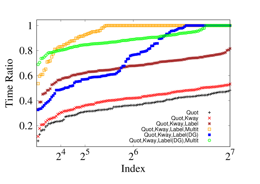
(b) Performance profile for running time (ordered running time ratios). Lower is better.

Figure 4: Comparing initial mapping algorithms from Table 2.

For the computation of initial mappings, we consider the six configurations listed in Table 2. Observe that Bsec and BsecN should apply either identity or top down depending on $k$. This choice is based on results obtained in [43] comparing these two OPMP construction algorithms. Figure 4 plots the results regarding solution quality and running time for our six configurations.

Looking at solution quality, the configurations using multisection dominate those using standard bisection except for instances having $k$ as a power of 2. This exception was expected since the standard bisection naturally performs a multisection partition for these instances. Among the configurations using multisection, identity produces overall better solutions than hierarchy top down, which is explained by the inherent locality of the multisection approach. Finally, the $N^{10}_{\mathcal{C}}$ local search is the least significant factor for solution quality, although it slightly improves solution compared to the similar configurations that skip local search.

In contrast to its low relevance for solution quality, the $N^{10}_{\mathcal{C}}$ local search is the dominant factor regarding running time. Observe that the configurations using identity are always the fastest ones among those algorithms that either use $N^{10}_{\mathcal{C}}$ local search or among those that don’t. Hence, the OPMP construction algorithm is the second most relevant factor for running time. Finally, the partitioning algorithm has little influence over running time, which reflects the rather small time difference between each of the pairs {BsecN, MsecTN} and {Bsec, MsecT}.

Since MsecIN has the best overall solution quality results, it is the natural choice for strong. Notice that MsecI has the best overall running times, which makes it the perfect choice for fast. Nevertheless, it is also the second best regarding solution quality, which suffices to make it also the best choice for eco.

Local Search.

For local search experiments, we start looking at the fast algorithm. To obtain a fast algorithm, we restrict its number of local search methods to one. Experiments with single local search algorithms do not yield much insight except that label propagation with delta-gain updates yields a very good trade-off for running time and solution quality.

(a) Improvements in objective function over Quot. Higher is better.

(b) Performance profile for running time (ordered running time ratios). Lower is better.

Figure 5: Results for local search experiment of the eco algorithm. It comprises four scenarios that represent successive additions of the respective local search methods. In (b), we show two additional scenarios in which delta-gain updates are used (represented by DG).

For the eco configuration of our algorithm, we build four configurations by incrementally inserting the local search methods. Additionally, we consider two extra configurations equipped with delta-gain updates during label propagation. Figure 5 summarizes the results concerning these six configurations. Since the behavior of strong in this experiment is equivalent, we omit its results without loss of completeness.

Figure 5 shows that solution quality and running time consistently increase after each consecutive addition of local refinement methods. Regarding delta gains, running times decrease for some values of $k$ but increase considerably and irregularly for others. Since this behavior is undesirable for eco, we drop delta gains for it. We also drop delta gains for strong since it does not affect solution quality and has negligible influence on running time compared to the $N^{10}_{\mathcal{C}}$ refinement. The clear choice for strong is the configuration with the four local searches since all of them contribute to incrementally improve solution quality. For eco, we drop only the multi-try FM local search since it adds little to solution quality but significantly increases the running time.

Distance Matrix.

Provided that the objective function is not influenced by the approach used to store or imply the distance matrix, the related experiments only show running time. We test four configurations: one with each of the three techniques that imply the distance matrix and a reference scenario in which we store the full distance matrix. Since all configurations of our algorithm display equivalent behavior, we focus on strong without loss of generality. Figure 6 plots a running time ratio chart for strong.

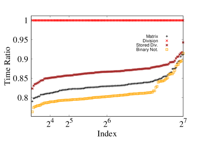
Figure 6: Performance plot for running times of different algorithm configurations (ordered running time ratios for different distance matrix implementations). Four alternative configurations are considered: implicit representations of the distance matrix based on division, stored division, and binary notation, and a reference scenario in which the matrix is explicitly stored. Lower is better.

It is easily understandable that the binary notation technique is faster than the stored division–based approach, and also that the latter is faster than the division–based approach. On the other hand, the binary notation outperforms the full-distance matrix approach. While both approaches allow O(1) distance calculations on our x86_64 architecture, accessing the distance matrix incurs a memory access. This leads to frequent cache misses since the $O(k^{2})$-sized distance matrix does not fit into the cache of our machine. Lastly, not using the distance matrix expectedly significantly improves the memory footprint of the algorithm. This especially prounced if the number of blocks gets very large. For example, for $2^{15}$ blocks, not using the distance matrix saves roughly an order of magnitude of necessary main memory.

4.2 Comparison with State of the Art

After the tuning step, the three configurations of our algorithm ended up as follows: (i) fast applies MsecI, label propagation with delta-gain updates, and binary notation; (ii) eco applies MsecI, quotient graph refinement, $k$-way FM, label propagation, and binary notation; and (iii) strong applies MsecIN, quotient graph refinement, $k$-way FM, label propagation, multi-try FM, and binary notation. To improve speed even more, we also include a configuration called fastest which applies MsecI as initial mapping, does not use any local search during uncoarsening, and never needs to use information from the distance matrix. In this section, we compare them against the best alternative algorithms in the literature. We report experiments on all graphs listed in Table 1 (excluding the graph used to tune our algorithm). In the evaluation we mostly compare the algorithm w.r.t. the baseline algorithm Müller-Merbach. At the end of this section, we highlight the comparison of various algorithms against each other.

We select the most successful algorithms from [43] and also Scotch for our comparison: (i) Top down with $N_{\mathcal{C}}^{d}$ local search (TopDownN), which represent the state-of-the-art for OPMP when $k$ is not a power of 2; (ii) identity mapping, which (when coupled with the KaHIP multilevel partitioning algorithm) represents the state-of-the-art for GPMP via two-phase approach when $k$ is a power of 2; (iii) the algorithm of Müller-Merbach [31] (Müller-Merbach), whose results are also used as a reference algorithm to calculate solution improvements in [43]; and (iv) Scotch [32]. We run the two-phase appraoches TopDownN, Identity, and Müller-Merbach coupled with K(Fast) as a partitioning algorithm. Since K(Fast)-TopDownN is our strongest competitor, we additionally couple TopDownN with K(Eco) and K(Strong) to obtain comparable running times. Recall that these algorithms are non-integrated: they use different quality configurations of KaHIP to partition the graph, compute the coarser communication model and then use TopDownN to compute a one-to-one mapping of blocks to processors (and hence of nodes to processors overall). Scotch is among the algorithms with best running times in our experiments. Hence, we add an algorithm (ScotchTC) which reports the best solution out of multiple runs of Scotch with different random seeds when given the same amount of time to compute a solution as our strong configuration has used. Figure 7 gives an overview over our results.

Regarding solution quality, our algorithms strong, eco, and fast dominate all the other approaches for most values of $k$. They respectively achieve average improvements of $72\%$, $69\%$, and $66\%$ over Müller-Merbach. TopDownN coupled with K(Strong), K(Eco), and K(Fast) generally produce the best solutions among our competitors. Their average improvements over Müller-Merbach are respectively $63\%$, $59\%$, and $53\%$. Our fastest algorithm comes next with an average improvement of $43\%$. Following are ScotchTC, Scotch, and K(Fast)-Identity, with improvements $24\%$, $23\%$, and $16\%$, respectively. When $k$ is a power of 2, our algorithms strong and eco are also the best, with average improvements over Müller-Merbach of $70\%$, $67\%$, respectively. They are followed by ScotchTC ($65\%$), Scotch and fast ($64\%$ each), K(Strong)-TopDownN ($63\%$), K(Eco)-TopDownN ($62\%$), K(Fast)-Identity ($57\%$), K(Eco)-TopDownN ($53\%$), and our algorithm fastest ($40\%$). Observe that some of our competitors produce solutions with higher average quality when $k$ is a power of 2. This happens because KaHIP and Scotch are based on recursive bisection schemes, which automatically partition throughout the hierarchy for such values of $k$.

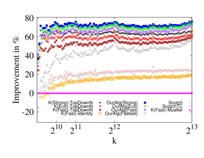
(a) Improvements in objective function over K(Fast)-Müller-Merbach. Higher is better.

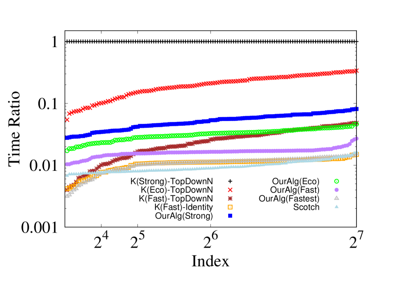
(b) Performance profile for running time. We omit ScotchTC, which equals OurAlg(Strong) in runtime. Lower is better.

Figure 7: Comparisons against state-of-the-art approaches for GPMP.

Scotch has the lowest average running time, directly followed by our algorithm fastest, K(Fast)-Identity, and our algorithm fast (respectively $9\%$, $10\%$, and $73\%$ slower than Scotch on average). Next, the average running time of K(Fast)-TopDownN is a factor $2.3$ higher than Scotch. For our algorithms eco and strong, this factor is respectively $3.3$ and $5.4$. By definition ScotchTC is also a factor $5.4$ higher than Scotch. K(Eco)-TopDownN has a much higher running time ($20.4$ times slower than Scotch). K(Strong)-TopDownN is our strongest competitor regarding solution quality but the slowest one ($107$ times slower than Scotch). Our fast, eco, and strong are respectively $62$, $32$, and $20$ times faster than K(Strong)-TopDownN, but still better than it regarding solution quality.

We now highlight various the comparison of various configurations/algorithms. The previously best approach in terms of overall mapping quality has been K(Strong)-TopDownN. Our strong configuration improves solution quality over K(Strong)-TopDownN by $5.1$% while being a factor $20$ on average faster. Our eco configuration has roughly $3.6\%$ better quality than K(Strong)-TopDown but is a factor $32$ faster on average. Our fast configuration still yields $1.3\%$ better solutions on average, and is a factor $62$ faster. Improved solution quality comes from the fact that the new algorithms are integrated and not two-phase, i. e., the multilevel algorithm directly optimize the correct objective. Improvements in running time are achieved since the KaHIP itself (which is used for partitioning) uses even more expensive local search algorithms such as flow-based improvement algorithms or global search schemes like V-cycles. Lastly, our fastest algorithm is on average $9\%$ slower than Scotch but also improves solution quality over Scotch by $16\%$.

5 Conclusion

As high-performance computing systems expand their processing power, there is also a growth regarding number of components, level of parallelism, and sophistication of the topology. In this work, we tackled the general process mapping problem, which consists of assigning a set of processes to a set of processing elements respecting an imbalance constraint in order to minimize the total communication cost between cores. Assuming a hierarchically organized topology and a sparse communication matrix containing much more processes than processing elements, we proposed, implemented, tuned, and tested integrated process mapping algorithms to tackle this problem.

We engineered all components of our novel algorithms within a multilevel scheme. Important ingredients of our algorithms include: (i) a recursive construction of initial solutions based on multisections throughout the hierarchy of processing elements; (ii) contraction-uncontraction schemes based on matchings; (iii) high-quality refinement methods such as label propagation, quotient graph refinement, and very localized local searches; (iv) a compressed structure to efficiently compute processor distances without storing a distance matrix; and (v) a memory scheme to keep delta-gain updates during label propagation in order to avoid recomputations of the objective function.

Experimental results indicate that our algorithms are the new state-of-the-art for general process mapping regarding solution quality. In particular, our algorithms generate much better overall solutions in comparison to any of their competitors while being faster than the previous best algorithm in terms of quality. Moreover, the best competitor regarding overall solution quality is, at the same time, slower and less effective than the simplest configuration of our algorithm. Our improvements are mostly due to the integrated multilevel approach combined with high-quality local search algorithms and initial mapping algorithms that split the initial network along the specified system hierarchy.

Important future work includes parallelization as well as the integration of global search schemes and different types of coarsening to improve solution quality further. Moreover, we want to investigate the impact that this new technology has on the real performance of applications such as sparse matrix vector multiplications. Lastly, we plan to release the proposed algorithms in the VieM (http://viem.taa.univie.ac.at/) and KaHIP (http://algo2.iti.kit.edu/kahip/) frameworks.

References

- Abdel-Gawad et al. [2014] A. H. Abdel-Gawad, M. Thottethodi, and A. Bhatele. RAHTM: Routing algorithm aware hierarchical task mapping. In Intl. Conference for High Performance Computing, Networking, Storage and Analysis (SC), pages 325–335, 2014.
- Andre et al. [2018] R. Andre, S. Schlag, and C. Schulz. Memetic multilevel hypergraph partitioning. In Proceedings of the Genetic and Evolutionary Computation Conference (GECCO), pages 347–354, 2018. 10.1145/3205455.3205475.
- Bader et al. [2014] D. A. Bader, H. Meyerhenke, P. Sanders, C. Schulz, A. Kappes, and D. Wagner. Benchmarking for graph clustering and partitioning. In Encyclopedia of Social Network Analysis and Mining, pages 73–82. Springer, 2014.
- Barnard and Simon [1993] S. T. Barnard and H. D. Simon. A fast multilevel implementation of recursive spectral bisection for partitioning unstructured problems. In Proc. of the 6th SIAM Conference on Parallel Processing for Scientific Computing, pages 711–718, 1993.
- Berti and Träff [2006] G. Berti and J. L. Träff. What MPI could (and cannot) do for mesh-partitioning on non-homogeneous networks. In Recent Advances in Parallel Virtual Machine and Message Passing Interface. 13th European PVM/MPI Users’ Group Meeting, volume 4192 of LNCS, pages 293–302. Springer Berlin Heidelberg, 2006.
- Bichot and Siarry [2011] C. Bichot and P. Siarry, editors. Graph Partitioning. Wiley, 2011.
- Blondel et al. [2008] V. D. Blondel, J. Guillaume, R. Lambiotte, and E. Lefebvre. Fast unfolding of community hierarchies in large networks. CoRR, abs/0803.0476, 2008. URL http://arxiv.org/abs/0803.0476.
- Brandfass et al. [2013] B. Brandfass, T. Alrutz, and T. Gerhold. Rank reordering for MPI communication optimization. Computers & Fluids, 80:372–380, 2013.
- Buluç et al. [2016] A. Buluç, H. Meyerhenke, I. Safro, P. Sanders, and C. Schulz. Recent Advances in Graph Partitioning, pages 117–158. Springer International Publishing, Cham, 2016. URL https://doi.org/10.1007/978-3-319-49487-6_4.
- Davis and Hu [2011] T. A. Davis and Y. Hu. The university of florida sparse matrix collection. ACM Trans. Math. Softw., 38(1):1:1–1:25, 2011. URL https://doi.org/10.1145/2049662.2049663.
- Delling et al. [2009a] D. Delling, R. Görke, C. Schulz, and D. Wagner. Orca reduction and contraction graph clustering. In Algorithmic Aspects in Information and Management, 5th International Conference, AAIM, volume 5564 of LNCS, pages 152–165. Springer, 2009a. 10.1007/978-3-642-02158-9_14.
- Delling et al. [2009b] D. Delling, P. Sanders, D. Schultes, and D. Wagner. Engineering route planning algorithms. In Algorithmics of Large and Complex Networks, volume 5515 of LNCS State-of-the-Art Survey, pages 117–139. Springer, 2009b.
- Fiduccia and Mattheyses [1982] C. M. Fiduccia and R. M. Mattheyses. A Linear-Time Heuristic for Improving Network Partitions. In Proc. of the 19th Conference on Design Automation, pages 175–181, 1982.
- Garey et al. [1974] M. R. Garey, D. S. Johnson, and L. Stockmeyer. Some Simplified NP-Complete Problems. In Proc. of the 6th ACM Symposium on Theory of Computing, (STOC), pages 47–63. ACM, 1974.
- Glantz et al. [2015] R. Glantz, H. Meyerhenke, and A. Noe. Algorithms for mapping parallel processes onto grid and torus architectures. In 23rd Euromicro Intl. Conference on Parallel, Distributed, and Network-Based Processing, pages 236–243, 2015.
- Glantz et al. [2018] R. Glantz, M. Predari, and H. Meyerhenke. Topology-induced enhancement of mappings. In Proceedings of the 47th International Conference on Parallel Processing, ICPP 2018, pages 9:1–9:10. ACM, 2018. 10.1145/3225058.3225117.
- Hager et al. [2018] W. W. Hager, J. T. Hungerford, and I. Safro. A multilevel bilinear programming algorithm for the vertex separator problem. Comp. Opt. and Appl., 69(1):189–223, 2018. 10.1007/s10589-017-9945-2.
- Hatazaki [1998] T. Hatazaki. Rank reordering strategy for MPI topology creation functions. In 5th European PVM/MPI User’s Group Meeting, volume 1497 of LNCS, pages 188–195, 1998.
- Heider [1972] C. H. Heider. A computationally simplified pair-exchange algorithm for the quadratic assignment problem. Technical report, DTIC Document, 1972.
- Hendrickson and Leland [1995] B. Hendrickson and R. Leland. A Multilevel Algorithm for Partitioning Graphs. In Proc. of the ACM/IEEE Conference on Supercomputing’95. ACM, 1995.
- Herrmann et al. [2019] J. Herrmann, M. Y. Özkaya, B. Uçar, K. Kaya, and Ü. V. Çatalyürek. Multilevel algorithms for acyclic partitioning of directed acyclic graphs. SIAM J. Scientific Computing, 41(4):A2117–A2145, 2019. 10.1137/18M1176865.
- Hoefler and Snir [2011] T. Hoefler and M. Snir. Generic topology mapping strategies for large-scale parallel architectures. In Proc. 25th Intl. Conf. on Supercomputing (ICS), pages 75–84. ACM, 2011.
- Karypis and Kumar [1998] G. Karypis and V. Kumar. A Fast and High Quality Multilevel Scheme for Partitioning Irregular Graphs. SIAM Journal on Scientific Computing, 20(1):359–392, 1998.
- Karypis and Kumar [1999] G. Karypis and V. Kumar. Multilevel k-way hypergraph partitioning. In Proceedings of the 36th Conference on Design Automation, pages 343–348, 1999. 10.1145/309847.309954.
- Mercier and Clet-Ortega [2009] G. Mercier and J. Clet-Ortega. Towards an efficient process placement policy for MPI applications in multicore environments. In 16th European Parallel Virtual Machine/Message Passing Interface Users’ Group Meeting, volume 5759 of LNCS, pages 104–115. Springer, 2009.
- Mercier and Jeannot [2011] G. Mercier and E. Jeannot. Improving MPI applications performance on multicore clusters with rank reordering. In 18th European MPI Users’ Group Meeting, volume 6960 of LNCS, pages 39–49. Springer, 2011.
- Meyerhenke et al. [2014] H. Meyerhenke, P. Sanders, and C. Schulz. Partitioning Complex Networks via Size-constrained Clustering. In 13th Int. Symp. on Exp. Algorithms, volume 8504 of LNCS. Springer, 2014.
- Meyerhenke et al. [2018] H. Meyerhenke, M. Nöllenburg, and C. Schulz. Drawing large graphs by multilevel maxent-stress optimization. IEEE Trans. Vis. Comput. Graph., 24(5):1814–1827, 2018. 10.1109/TVCG.2017.2689016.
- Moreira et al. [2017] O. Moreira, M. Popp, and C. Schulz. Graph partitioning with acyclicity constraints. In 16th International Symposium on Experimental Algorithms, (SEA), volume 75 of LIPIcs, pages 30:1–30:15, 2017. 10.4230/LIPIcs.SEA.2017.30.
- Moreira et al. [2018] O. Moreira, M. Popp, and C. Schulz. Evolutionary multi-level acyclic graph partitioning. In Proceedings of the Genetic and Evolutionary Computation Conference, (GECCO), pages 332–339, 2018. 10.1145/3205455.3205464.
- Müller-Merbach [1970] H. Müller-Merbach. Optimale reihenfolgen, volume 15 of Ökonometrie und Unternehmensforschung. Springer-Verlag, 1970.
- [32] F. Pellegrini. Scotch Home Page. http://www.labri.fr/pelegrin/scotch.
- Pellegrini and Roman [1996] F. Pellegrini and J. Roman. SCOTCH: A software package for static mapping by dual recursive bipartitioning of process and architecture graphs. In High-Performance Computing and Networking, volume 1067 of Lecture Notes in Computer Science, pages 493–498. Springer, 1996. 10.1007/3-540-61142-8_588.
- Raghavan et al. [2007] U. N. Raghavan, R. Albert, and S. Kumara. Near linear time algorithm to detect community structures in large-scale networks. Physical Review E, 76(3):036106, 2007.
- Sahni and Gonzalez [1976] S. Sahni and T. F. Gonzalez. P-complete approximation problems. J. ACM, 23(3):555–565, 1976. URL http://doi.acm.org/10.1145/321958.321975.
- [36] P. Sanders and C. Schulz. KaHIP – Karlsruhe High Qualtity Partitioning Homepage. http://algo2.iti.kit.edu/documents/kahip/index.html.
- Sanders and Schulz [2011] P. Sanders and C. Schulz. Engineering Multilevel Graph Partitioning Algorithms. In Proc. of the 19th European Symp. on Algorithms, volume 6942 of LNCS, pages 469–480. Springer, 2011.
- Sanders and Schulz [2013] P. Sanders and C. Schulz. Think Locally, Act Globally: Highly Balanced Graph Partitioning. In 12th Intl. Sym. on Experimental Algorithms (SEA), LNCS. Springer, 2013.
- Sanders and Schulz [2016] P. Sanders and C. Schulz. Advanced multilevel node separator algorithms. In Experimental Algorithms - 15th International Symposium, (SEA), Proceedings, volume 9685 of LNCS, pages 294–309. Springer, 2016. 10.1007/978-3-319-38851-9_20.
- Schlag et al. [2016] S. Schlag, V. Henne, T. Heuer, H. Meyerhenke, P. Sanders, and C. Schulz. k-way hypergraph partitioning via n-level recursive bisection. In Proceedings of the Eighteenth Workshop on Algorithm Engineering and Experiments, ALENEX, pages 53–67, 2016. 10.1137/1.9781611974317.5.
- Schulz [2013] C. Schulz. High Quality Graph Partititioning. PhD thesis, Karlsruhe Institute of Technology, 2013.
- Schulz and Strash [2019] C. Schulz and D. Strash. Graph partitioning: Formulations and applications to big data. In S. Sakr and A. Y. Zomaya, editors, Encyclopedia of Big Data Technologies. Springer, 2019. URL https://doi.org/10.1007/978-3-319-63962-8_312-2.
- Schulz and Träff [2017] C. Schulz and J. L. Träff. Better process mapping and sparse quadratic assignment. In 16th International Symposium on Experimental Algorithms, volume 75 of LIPIcs, pages 4:1–4:15, 2017. 10.4230/LIPIcs.SEA.2017.4.
- Soper et al. [2004] A. J. Soper, C. Walshaw, and M. Cross. A Combined Evolutionary Search and Multilevel Optimisation Approach to Graph-Partitioning. Global Optimization, 29(2):225–241, 2004.
- Southwell [1935] R. V. Southwell. Stress-Calculation in Frameworks by the Method of “Systematic Relaxation of Constraints”. Proc. of the Royal Society of London, 151(872):56–95, 1935.
- Träff [2002] J. L. Träff. Implementing the MPI process topology mechanism. In ACM/IEEE Supercomputing, pages 40:1–40:14, 2002.
- Vogelstein et al. [2015] J. T. Vogelstein, J. M. Conroy, V. Lyzinski, L. J. Podrazik, S. G. Kratzer, E. T. Harley, D. E. Fishkind, R. J. Vogelstein, and C. E. Priebe. Fast approximate quadratic programming for graph matching. PLOS One, April 2015.
- von Kirchbach et al. [2019] K. von Kirchbach, C. Schulz, and J. L. Träff. Better process mapping and sparse quadratic assignment. CoRR, 2019. URL http://arxiv.org/abs/1702.04164v2.
- Walshaw [2003] C. Walshaw. A multilevel algorithm for force-directed graph-drawing. J. Graph Algorithms Appl., 7(3):253–285, 2003. URL https://doi.org/10.7155/jgaa.00070.
- Walshaw and Cross [2000] C. Walshaw and M. Cross. Mesh Partitioning: A Multilevel Balancing and Refinement Algorithm. SIAM Journal on Scientific Computing, 22(1):63–80, 2000.
- Walshaw and Cross [2001] C. Walshaw and M. Cross. Multilevel mesh partitioning for heterogeneous communication networks. Future Generation Comp. Syst., 17(5):601–623, 2001. URL https://doi.org/10.1016/S0167-739X(00)00107-2.
- Yu et al. [2006] H. Yu, I.-H. Chung, and J. E. Moreira. Topology mapping for Blue Gene/L supercomputer. In ACM/IEEE Supercomputing, page 116, 2006.