Multiplication fusion of sparse and collaborative-competitive representation for image classification

Abstract

Representation based classification methods have become a hot research topic during the past few years, and the two most prominent approaches are sparse representation based classification (SRC) and collaborative representation based classification (CRC). CRC reveals that it is the collaborative representation rather than the sparsity that makes SRC successful. Nevertheless, the dense representation of CRC may not be discriminative which will degrade its performance for classification tasks. To alleviate this problem to some extent, we propose a new method called sparse and collaborative-competitive representation based classification (SCCRC) for image classification. Firstly, the coefficients of the test sample are obtained by SRC and CCRC, respectively. Then the fused coefficient is derived by multiplying the coefficients of SRC and CCRC. Finally, the test sample is designated to the class that has the minimum residual. Experimental results on several benchmark databases demonstrate the efficacy of our proposed SCCRC. The source code of SCCRC is accessible at https://github.com/li-zi-qi/SCCRC.

1 Introduction

Representation based classification methods (RBCM) have already gained increasing attention in various research fields, e.g. character recognition qu2018air , person re-identification prates2019kernel and hyperspectral image classification yang2018hyperspectral . SRC wright2009robust is a pioneering work of RBCM, which directly uses all the training data as the dictionary to represent the test sample, and classifies the test sample by checking which class leads to the minimal reconstruction error. SRC solves an $\ell_{1}$-norm optimization problem, and thus when the size of dictionary is huge, the sparse decomposition process may be very slow. One way to speed up the sparse coding process is to reduce the size of dictionary by selecting representative training samples. Li et al.li2010local proposed a local sparse representation based classification (LSRC) scheme, which performs sparse decomposition in local neighborhood. Similarly, Zhang et al.zhang2010k presented KNN-SRC, which chooses $K$ nearest neighbors of a testing sample from all the training samples to represent the testing sample. Ortiz et al.ortiz2014face developed a linearly approximated sparse representation-based classification (LASRC) algorithm that employs linear regression to perform sample selection for $\ell_{1}$-minimization. The other way is to obtain a compact and discriminative dictionary through dictionary learning. The most classic dictionary learning approach is KSVD aharon2006k , which is an iterative method that alternates between sparse coding and a process of updating the dictionary atoms. To make KSVD more suitable for classification tasks, Zhang et al.zhang2010discriminative proposed a discriminative K-SVD (D-KSVD) method which incorporates the classification error into the objective function of KSVD. Jiang et al.jiang2013label presented a label consistent K-SVD (LC-KSVD) algorithm which combines a new label consistency constraint with the reconstruction error and the classification error to form a unified objective function. Later Kviatkovsky et al.kviatkovsky2017equivalence proved that under identical initialization conditions, LC-KSVD with uniform atom allocation is essentially a reformulation of DKSVD. Very recently, Song et al.song2018euler designed a kernel dictionary learning approach called Euler Label Consistent K-SVD (ELC-KSVD) to capture the nonlinear similarity of features.

Another prominent approach of RBCM is CRC zhang2011sparse which replaces the $\ell_{1}$-norm in SRC with $\ell_{2}$-norm. Furthermore, Zhang et al.zhang2011sparse revealed that it is the collaborative representation (CR) mechanism, but not the $\ell_{1}$-norm sparsity that makes SRC successful for classification. Likewise, Xu et al.xu2017new introduced a discriminative sparse representation (DSR) method for robust face recognition via $\ell_{2}$ regularization. The representation fidelity term in DSR is measured by $\ell_{2}$-norm. To enhance the robustness of DSR, Zeng et al.zeng2017antinoise proposed a robust version of DSR called Antinoise sparse representation method based on joint $\ell_{1}$ and $\ell_{2}$ regularization (Anti-L1L2) by employing the $\ell_{1}$-norm to measure the fidelity term. Although CRC presents a geometric interpretation of its working mechanism, it is hard to understand. Afterwards, Cai et al.cai2016probabilistic analyzed the classification mechanism of CRC from a probabilistic viewpoint and proposed a probabilistic collaborative representation based classifier (ProCRC). Based on ProCRC, Lan et al.lan2018prior explored a method called prior knowledge-based probabilistic CRC (PKPCRC) with further consideration of the prior knowledge extracted from the training samples. Yuan et al.yuan2018collaborative constructed a collaborative-competitive representation based classifier (CCRC) model by introducing a competitive regularization term into the objective function of CRC. Using the training samples of all classes to collaboratively represent a test sample may produce negative effect, to overcome this problem, Zheng et al.zheng2019collaborative presented a $k$-nearest classes based classification scheme. Moreover, Waqas et al.waqas2013collaborative proposed a method known as collaborative neighbor representation classifier (CNRC) which represents a test sample over the whole training dictionary by automatically selecting bases from the training samples close to test sample. By integrating CNRC and DSR, Gou et al.gou2018new designed a new discriminative collaborative neighbor representation (DCNR) method for face recognition.

The above RBCM and their variants emphasize too much on the role of $\ell_{1}$-norm sparsity or collaborative representation, and thus researchers are seeking to find new ways of combining them to enhance the performance of classification. Akhtar et al.akhtar2017efficient argued that sparseness of collaborative representation explicitly contributes to accurate classification, and they developed a sparsity augmented collaborative representation based classification (SA-CRC) scheme. Zeng et al.zeng2017multiplication proposed a representation-based image classification method that integrates SRC with CRC by a multiplication operation on the solutions. Li et al.li2016hyperspectral presented a fused representation-based classification (FRC) method which attempts to achieve the balance between CR and SR in the residual domain. However, there is a weight parameter in FRC which needs to be set manually. Furthermore, the results in  akhtar2017efficient demonstrate that sparsity of collaborative representation does play a critical role in the correct classification of test samples. By multiplying the coefficient vectors obtained by SRC and CRC, sparsity of the fused coefficient vector in SCRC zeng2017multiplication is enhanced to some extent. Unfortunately, the coefficient vector obtained by CRC is limited sparse. In order to further promote the sparsity of fused coefficient vector, in this paper, we propose a new method coined sparse and collaborative-competitive representation based classification (SCCRC) for image classification. The fused coefficient is obtained by multiplying the coefficients of SRC and CCRC, and then the test sample is classified by checking which class yields the least residual. Some representative RBCM and our proposed SCCRC are summarized in Table 1, and our main contributions are summarized as follows,

1. Our proposed SCCRC involves the multiplication of coefficients obtained by SRC and CCRC, it does not need to determine additional parameters, which makes SCCRC very efficient.

2. Although SCCRC is simple in principle, it outperforms some state-of-the-art RBCM on both clean and corrupted images in terms of classification accuracy.

3. Statistical significance test indicates that the performance differences between SCCRC and all the competing approaches are statistically significant.

Table 1: Summarization of some representative RBCM. Note that in FRC, the residuals obtained by SRC and CRC are fused by a weghting parameter $\theta$. In SCRC and SA-CRC, $\hat{\boldsymbol{\alpha}}$ and $\check{\boldsymbol{\alpha}}$ are the coefficient vectors obtained by SRC and CRC, respectively. In our proposed SCCRC, $\boldsymbol{\alpha}$ and $\boldsymbol{\beta}$ are the coefficient vectors obtained by SRC and CCRC, respectively.

Algorithm	Formulation
SRC wright2009robust	$\underset{\boldsymbol{\alpha}}{\min}\left\{\left\|\boldsymbol{y}-\mathbf{X}\boldsymbol{\alpha}\right\|_{2}^{2}+\lambda\left\|\boldsymbol{\alpha}\right\|_{1}\right\}$
CRC zhang2011sparse	$\underset{\boldsymbol{\alpha}}{\min}\left\{\left\|\boldsymbol{y}-\mathbf{X}\boldsymbol{\alpha}\right\|_{2}^{2}+\lambda\left\|\boldsymbol{\alpha}\right\|_{2}^{2}\right\}$
FRC li2016hyperspectral	$\boldsymbol{r}=(1-\theta)\left\|\boldsymbol{y}-\mathbf{X}_{i}\boldsymbol{\hat{\alpha}_{i}}\right\|_{2}+\theta\left\|\boldsymbol{y}-\mathbf{X}_{i}\boldsymbol{\check{\alpha}_{i}}\right\|_{2}$
SCRC zeng2017multiplication	$\boldsymbol{f}=\hat{\boldsymbol{\alpha}}\odot\check{\boldsymbol{\alpha}}$
NRC xu2019sparse	$\underset{\boldsymbol{\alpha}}{\min}\left\|\boldsymbol{y}-\mathbf{X}\boldsymbol{\alpha}\right\|_{2}^{2},\ \textrm{s.t.}\ \boldsymbol{\alpha}\geq 0$
SA-CRC akhtar2017efficient	$\stackrel{{\scriptstyle\circ}}{{\boldsymbol{\alpha}}}=\frac{\hat{\boldsymbol{\alpha}}+\check{\boldsymbol{\alpha}}}{\left\|\hat{\boldsymbol{\alpha}}+\check{\boldsymbol{\alpha}}\right\|_{2}}$
CCRC yuan2018collaborative	$\underset{\boldsymbol{\beta}}{\textrm{min}}\left\{\|\boldsymbol{y}-\mathbf{X}\boldsymbol{\beta}\|_{2}^{2}+\lambda_{1}\|\boldsymbol{\beta}\|_{2}^{2}+\lambda_{2}\sum_{i=1}^{C}\left\|\boldsymbol{y}-\mathbf{X}_{i}\boldsymbol{\beta}_{i}\right\|_{2}^{2}\right\}$
SCCRC	$\boldsymbol{f}=\boldsymbol{\alpha}\odot\boldsymbol{\beta}$

The remainder of this paper is structured as follows: Section 2 introduces several related approaches which include SRC, CRC, LRC naseem2010linear and CCRC. Section 3 presents our SCCRC algorithm. Section 4 reports the experiments on several benchmark databases. Finally, Section 5 concludes the paper.

2 Related work

As our SCCRC is based on SRC and CCRC, we now briefly review these approaches for the sake of completeness.

We consider a set of $n$ training samples collected from $C$ subjects, each training image is represented as a vector corresponding to the $i$th column of the dictionary. Thus, all training samples form the matrix $\mathbf{X}=\left[\mathbf{X}_{1},\mathbf{X}_{2},\ldots,\mathbf{X}_{C}\right]\in\mathbb{R}^{d\times n}$ and $\mathbf{X}_{i}=\left[\mathbf{X}_{i,1},\mathbf{X}_{i,2},\ldots,\mathbf{X}_{i,n_{i}}\right]\in\mathbb{R}^{d\times n_{i}},i=1,2,\ldots,C$, where $d$ is the dimensionality of each sample and $n_{i}$ denotes the number of training samples in the $i$th class.

2.1 Sparse representation based classification

Given a test sample $\boldsymbol{y}\in\mathbb{R}^{d\times 1}$, SRC employs a sparse linear superposition of all the training data to represent the test sample by solving the following $\ell_{1}$-norm minimization problem,

$$\underset{\boldsymbol{\alpha}}{\min}\left\{\left\|\boldsymbol{y}-\mathbf{X}\boldsymbol{\alpha}\right\|_{2}^{2}+\lambda\left\|\boldsymbol{\alpha}\right\|_{1}\right\}$$ (1)

where $\lambda>0$ is a balancing parameter. Then the reconstruction error (residual) for each class is obtained by,

$$\boldsymbol{r}_{i}=\left\|\boldsymbol{y}-\mathbf{X}_{i}\boldsymbol{\hat{\alpha}_{i}}\right\|_{2}$$ (2)

where $\boldsymbol{\hat{\alpha}_{i}}$ is the coefficients that correspond to the $i$th class. Finally, the identity of the test sample $\boldsymbol{y}$ is determined by evaluating which class leads to the least residual, i.e.

$$\textrm{identity}\left(\boldsymbol{y}\right)=\underset{i}{\min}~{}\boldsymbol{r}_{i}$$ (3)

2.2 Collaborative representation based classification

CRC estimates the representation of the test sample $\boldsymbol{y}$ by relaxing the $\ell_{1}$-norm to the $\ell_{2}$-norm in (1). The objective function of CRC is formulated as follows,

$$\underset{\boldsymbol{\alpha}}{\min}\left\{\left\|\boldsymbol{y}-\mathbf{X}\boldsymbol{\alpha}\right\|_{2}^{2}+\lambda\left\|\boldsymbol{\alpha}\right\|_{2}^{2}\right\}$$ (4)

where $\lambda>0$ is a balancing parameter. Eq. (4) has closed form solution $\hat{\boldsymbol{\alpha}}=\left(\mathbf{X}^{T}\mathbf{X}+\lambda\mathbf{I}\right)^{-1}\mathbf{X}^{T}\boldsymbol{y}$. In zhang2011sparse , Zhang found that in addition to the residual, the classwise coefficients $\boldsymbol{\hat{\alpha}_{i}}$ can also bring some discrimination information for classification. Therefore, they proposed the following regularized residual for classification,

$$\boldsymbol{r}_{i}=\frac{\left\|\boldsymbol{y}-\mathbf{X}_{i}{\boldsymbol{\hat{\alpha}}_{i}}\right\|_{2}}{\left\|{\boldsymbol{\hat{\alpha}}}_{i}\right\|_{2}}$$ (5)

2.3 Linear regression classification

Different from SRC and CRC which employ all the training samples for representation, the mechanism of LRC adopts the training samples in each class to reconstruct the test sample $\boldsymbol{y}$ in a classwise manner. Specifically, the objective function of LRC is formulated as,

$$\underset{\boldsymbol{\alpha}_{i}}{\min}\left\|\boldsymbol{y}-\mathbf{X}_{i}\boldsymbol{\alpha}_{i}\right\|_{2}^{2}$$ (6)

Eq. (6) has closed-form solution, which is given by,

$${\boldsymbol{\hat{\alpha}}_{i}}=\left({\mathbf{X}}_{i}^{T}{\mathbf{X}}_{i}\right)^{-1}\mathbf{X}_{i}^{T}\boldsymbol{y}$$ (7)

Finally, the test sample $\boldsymbol{y}$ is classified according to the following rule,

$$\textrm{identity}(\boldsymbol{y})=\underset{i}{\min}\left\|\boldsymbol{y}-{\mathbf{X}}_{i}{\boldsymbol{\hat{\alpha}}_{i}}\right\|_{2}$$ (8)

In fact, the essence of LRC is nearest subspace (NS) classifier with downsampled features.

2.4 Collaborative-competitive representation based classification (CCRC)

Yuan et al.yuan2018collaborative proposed a collaborative-competitive representation based classifier model (CCRC) which incorporates a competitive term into the formulation of CRC, and the objective function of CCRC is formulated as follows,

$$\min_{\boldsymbol{\beta}}\left\{\|\boldsymbol{y}-\mathbf{X}\boldsymbol{\beta}\|_{2}^{2}+\lambda_{1}\|\boldsymbol{\beta}\|_{2}^{2}+\lambda_{2}\sum_{i=1}^{C}\left\|\boldsymbol{y}-\mathbf{X}_{i}\boldsymbol{\beta}_{i}\right\|_{2}^{2}\right\}$$ (9)

where $\|\boldsymbol{y}-\mathbf{X}\boldsymbol{\beta}\|_{2}^{2}$ aims to collaboratively express the test sample by using all the training samples, $\sum_{i=1}^{C}\left\|\boldsymbol{y}-\mathbf{X}_{i}\boldsymbol{\beta}_{i}\right\|_{2}^{2}$ encourages the competitive representation across different classes, $\lambda_{1}$ and $\lambda_{2}$ are balancing parameters. As we can see from Eq. (9), if $\lambda_{2}$ equals to 0, CCRC boils down to CRC. CCRC has closed-form solution, which is given by,

$$\boldsymbol{\beta}=\mathbf{P}\boldsymbol{y}$$ (10)

where $\mathbf{P}=\left(1+\lambda_{2}\right)\left(\mathbf{X}^{T}\mathbf{X}+\lambda_{1}\mathbf{I}+\lambda_{2}\mathbf{M}\right)^{-1}\mathbf{X}^{T}$ and $\mathbf{M}=\left[\begin{array}[]{ccc}{\mathbf{X}_{1}^{T}\mathbf{X}_{1}}&{\cdots}&{0}\\ {\vdots}&{\ddots}&{\vdots}\\ {0}&{\cdots}&{\mathbf{X}_{C}^{T}\mathbf{X}_{C}}\end{array}\right]$

3 Sparse and collaborative-competitive representation based classification

3.1 SCCRC method

Although CRC and its improved approaches achieve impressive results in various classification tasks, it does not mean that sparsity can be totally ignored. Deng et al.deng2013defense pointed out that the dense coefficient of CRC would mislead the classification, and in a more recent work deng2018face , they find that when given uncontrolled and limited training data, the $\ell_{1}$-minimization technique obtains more desirable results than that of $\ell_{2}$-norm. Akhtar et al.akhtar2017efficient also argued that sparsity plays an explicit role in accurate classification and they proposed a sparsity augmented collaborative representation based classification (SA-CRC) algorithm. Inspired by the above work, we present sparse and collaborative-competitive representation based classification (SCCRC) method which combines sparse and collaborative-competitive representation for classification. Concretely, we first obtain the coefficients of test sample by SRC and CCRC, respectively. Then the two coefficients are fused by element-wise multiplication. Finally, we classify the test sample to the class that has the minimal residual. The detailed procedures of our SCCRC is summarized in Algorithm 1.

Algorithm 1 SCCRC

0:  training data matrix $\mathbf{X}$, test data $\boldsymbol{y}$, parameter $\lambda$ for SRC, parameters $\lambda_{1}$ and $\lambda_{2}$ for CCRC.

1:  Compute the sparse coefficient $\boldsymbol{\alpha}$ of test sample $\boldsymbol{y}$ according to Eq. (1);

2:  Obtain the coefficient of CCRC $\boldsymbol{\beta}$ for $\boldsymbol{y}$ based on Eq. (10);

3:  Compute the fused coefficient $\boldsymbol{f}=\boldsymbol{\alpha}\odot\boldsymbol{\beta}$;

4:  Classify $\boldsymbol{y}$ to the class that has the least residual: $\textrm{identity}(\boldsymbol{y})=\underset{i}{\min}\left\|\boldsymbol{y}-\mathbf{X}_{i}\boldsymbol{f}_{i}\right\|_{2}$;

4:  the identity of $\boldsymbol{y}$.

3.2 Difference between SCCRC and CCRC-$\ell_{1}$

Our proposed SCCRC aims to promote the sparsity of coefficient vector obtained by CCRC, which involves a simple multiplication of coefficient vectors derived by SRC and CCRC. Another intuitive way to increase the sparsity of coefficient vector of CCRC is modifying the objective function of CCRC, i.e., replacing the $\ell_{2}$-norm constraint on $\boldsymbol{\beta}$ with the $\ell_{1}$-norm. This method is called CCRC-$\ell_{1}$, and its objective function is formulated as follows,

$$\underset{\boldsymbol{\beta}}{\textrm{min}}\left\{\|\boldsymbol{y}-\mathbf{X}\boldsymbol{\beta}\|_{2}^{2}+\lambda_{1}\|\boldsymbol{\beta}\|_{1}+\lambda_{2}\sum_{i=1}^{C}\left\|\boldsymbol{y}-\mathbf{X}_{i}\boldsymbol{\beta}_{i}\right\|_{2}^{2}\right\}$$ (11)

To solve Eq. (11), by introducing an auxiliary variable $\boldsymbol{z}$, Eq. (11) can be converted into the following equivalent optimization problem,

$$\underset{\boldsymbol{\beta},\boldsymbol{z}}{\textrm{min}}\left\{\|\boldsymbol{y}-\mathbf{X}\boldsymbol{\beta}\|_{2}^{2}+\lambda_{1}\|\boldsymbol{z}\|_{1}+\lambda_{2}\sum_{i=1}^{C}\left\|\boldsymbol{y}-\mathbf{X}_{i}\boldsymbol{\beta}_{i}\right\|_{2}^{2}\right\},\ \textrm{s.t.}\ \boldsymbol{\beta}=\boldsymbol{z}$$ (12)

The Augmented Lagrange Multiplier (ALM) scheme can be adopted to solve Eq. (12), and the augmented Langrangian function is formulated as,

$$\mathcal{L}(\boldsymbol{\beta},\boldsymbol{z},\boldsymbol{\theta},\mu)=\|\boldsymbol{y}-\mathbf{X}\boldsymbol{\beta}\|_{2}^{2}+\lambda_{1}\|\boldsymbol{z}\|_{1}+\lambda_{2}\sum_{i=1}^{C}\left\|\boldsymbol{y}-\mathbf{X}_{i}\boldsymbol{\beta}_{i}\right\|_{2}^{2}+\left\langle\boldsymbol{\theta},\boldsymbol{\beta}-\boldsymbol{z}\right\rangle+\frac{\mu}{2}\left\|\boldsymbol{\beta}-\boldsymbol{z}\right\|_{2}^{2}$$ (13)

where $\boldsymbol{\theta}$ is the Lagrange multiplier, and $\mu>0$ is a penalty parameter. Eq. (13) can be solved iteratively by updating $\boldsymbol{\beta}$ and $\boldsymbol{z}$ once at a time. The detailed procedures are presented as follows.

Update $\boldsymbol{\beta}$: Fix $\boldsymbol{z}$ and update $\boldsymbol{\beta}$ by solving the following problem,

$$\underset{\boldsymbol{\beta}}{\textrm{min}}\ \|\boldsymbol{y}-\mathbf{X}\boldsymbol{\beta}\|_{2}^{2}+\lambda_{2}\sum_{i=1}^{C}\left\|\boldsymbol{y}-\mathbf{X}_{i}\boldsymbol{\beta}_{i}\right\|_{2}^{2}+\left\langle\boldsymbol{\theta},\boldsymbol{\beta}-\boldsymbol{z}\right\rangle+\frac{\mu}{2}\left\|\boldsymbol{\beta}-\boldsymbol{z}\right\|_{2}^{2}$$ (14)

Suppose $\mathbf{X}_{i}^{{}^{\prime}}$ is a matrix that has the same size as $\mathbf{X}$, and $\mathbf{X}_{i}^{{}^{\prime}}$ only consists of samples from the $i$-th class, i.e., $\mathbf{X}_{i}^{{}^{\prime}}=[\boldsymbol{0},\ldots,\mathbf{X}_{i},\ldots,\boldsymbol{0}]$, Equation (14) can be reformulated as,

$$\underset{\boldsymbol{\beta}}{\textrm{min}}\ \|\boldsymbol{y}-\mathbf{X}\boldsymbol{\beta}\|_{2}^{2}+\lambda_{2}\sum_{i=1}^{C}\left\|\boldsymbol{y}-\mathbf{X}_{i}^{{}^{\prime}}\boldsymbol{\beta}\right\|_{2}^{2}+\frac{\mu}{2}\left\|\boldsymbol{\beta}-\boldsymbol{z}+\frac{\boldsymbol{\theta}}{\mu}\right\|_{2}^{2}$$ (15)

which has the following closed-form solution,

$$\boldsymbol{\beta}=\left[\mathbf{X}^{T}\mathbf{X}+\lambda_{2}\sum_{i=1}^{C}(\mathbf{X}_{i}^{{}^{\prime}})^{T}\mathbf{X}_{i}^{{}^{\prime}}+\frac{\mu}{2}\mathbf{I}\right]^{-1}((1+\lambda_{2})\mathbf{X}^{T}\boldsymbol{y}+\frac{\mu\boldsymbol{z}-\boldsymbol{\theta}}{2})$$ (16)

where $\mathbf{I}$ is an identity matrix.

Update $\boldsymbol{z}$: Fix $\boldsymbol{\boldsymbol{\beta}}$ and update $\boldsymbol{z}$ by solving the following problem,

$$\underset{\boldsymbol{z}}{\textrm{min}}\ \frac{\lambda_{1}}{\mu}\left\|\boldsymbol{z}\right\|_{1}+\frac{1}{2}\left\|\boldsymbol{z}-(\boldsymbol{\beta}+\frac{\boldsymbol{\theta}}{\mu})\right\|$$ (17)

Eq. (17) can be solved by the soft-thresholding operator combettes2005signal . The complete procedures of solving Eq. (12) are summarized in Algorithm 2.

Algorithm 2 Solve Eq. (12) via ALM

0:  Test sample $\boldsymbol{y}$, training data matrix $\mathbf{X}$, balancing parameter $\lambda_{1}$ and $\lambda_{2}$.

1:  Initialize $\boldsymbol{z}=\boldsymbol{\theta}=\boldsymbol{0}$, $\mu=0.5$, $\mu_{\textrm{max}}=10^{6}$, $\rho=1.1$, $\varepsilon=10^{-3}$;

2:  while not converged do

3:     Update $\boldsymbol{\beta}$ by Eq. (16);

4:     Update $\boldsymbol{z}$ by solving Eq. (17);

5:     Update $\boldsymbol{\theta}$ by $\boldsymbol{\theta}=\boldsymbol{\theta}+\mu(\boldsymbol{\beta}-\boldsymbol{z})$;

6:     Update $\mu$ by $\mu=\textrm{min}(\rho\mu,\mu_{\textrm{max}})$;

7:     Check the convergence condiction: $\left\|\boldsymbol{\beta}-\boldsymbol{z}\right\|_{\infty}<\varepsilon$.

8:  end while

8:  Coefficient vector $\boldsymbol{\beta}$.

From Eq. (11), one can see that CCRC-$\ell_{1}$ directly imposes the $\ell_{1}$-norm constraint on the coefficient vector $\boldsymbol{\beta}$, and the $\ell_{1}$-norm constraint induces sparsity of $\boldsymbol{\beta}$. CCRC-$\ell_{1}$ is solved by ALM, which iteratively update the variables. By contrast, our proposed SCCRC is more straightforward, it fuses the coefficients of SRC and CCRC by multiplication. Note that coefficient vectors of test data can be viewed as some kind of features, and the multiplication fusion of coefficient vectors is equivalent to the data integration at the feature level. We believe that the feature level fusion can bring in improved performance, as demonstrated by the experimental results in Section 4.

3.3 Rationale of SCCRC

In our proposed SCCRC, the fused coefficient vector of a test sample $\boldsymbol{y}$ is derived by $\boldsymbol{f}=\boldsymbol{\alpha}\odot\boldsymbol{\beta}$, where $\boldsymbol{\alpha}$ and $\boldsymbol{\beta}$ are obtained by SRC and CCRC, respectively. According to the procedures of SRC and CCRC, the test sample $\boldsymbol{y}$ and training data matrix $\mathbf{X}$ are normalized to have unit $\ell_{2}$-norm. Therefore, absolute values of the entries in the coefficient vectors are less than 1. When both the elements in $\boldsymbol{\alpha}$ and $\boldsymbol{\beta}$ have large absolute value, after multiplication, the corresponding element in $\boldsymbol{f}$ will also have large absolute value. In most cases, coefficient vector obtained by SRC is sparse, while the coefficient vector obtained by CCRC is a little dense, and coefficients of the training samples, whose labels are the same as the test sample, tend to have large absolute value. Therefore, sparsity of the fused coefficient vector is promoted which is beneficial for the correct classification of the test sample.

To vividly illustrate the effectiveness of SCCRC, we here present an example on the ORL database. We choose a test image from the 28th subject, and the training data consists of the first 3 images per person, and thus the dictionary contains $40\times 3=120$ atoms. Fig. 1 shows the coefficients obtained by SRC, and the prominent coefficients correspond to the 28th class. Fig. 2 depicts the reconstruction error for each class, and the 28th class has the least residual, so the test sample is correctly classified. Fig. 3 plots the coefficients computed by CCRC, we can find that the largest coefficient corresponds to the 28th class. However, when we check the residual presented in Fig. 4, the test sample is wrongly classified into the 6th class. The reason is that the other two coefficients of the 28th subject are negative, which leads to the fact that the 28th class does not produce the least residual. Fig. 5 shows the coefficients computed by our SCCRC, we can see that by fusing the coefficients of SRC and CCRC, the dominant coefficients correspond to the 28th class. Though the other two coefficients are negative, they are relatively small compared with the positive one. Thus, the residual of the 28th subject is the minimal, which is illustrated in Fig. 6. By comparing Fig. 5 with Figs. 1 and 3, we can observe that the fused coefficient vector of SCCRC is more sparse than that of SRC and CCRC, which validates the effectiveness of multiplication fusion.

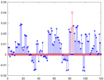
Figure 1: Coefficients computed by SRC, we can see that the prominent coefficients concentrate on the correct class (the 28th class).

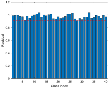
Figure 2: The residual obtained by SRC, and the 28th class has the least residual.

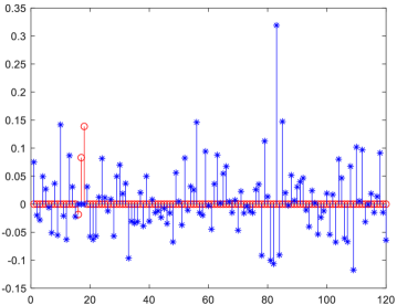
Figure 3: Coefficients computed by CCRC, although the 28th class has the largest coefficient, the other two coefficients are negative. In fact, the test sample is wrongly classified into the 6th class.

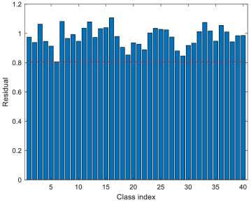
Figure 4: The residual obtained by CCRC, and the 6th class has the least residual. As a result, the test sample is misclassified.

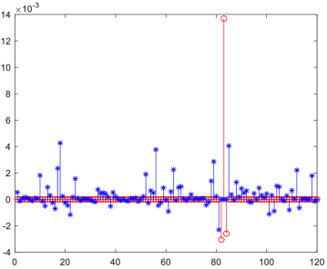
Figure 5: Coefficients computed by SCCRC, we can see that the dominant coefficients correspond to the correct class (the 28th class).

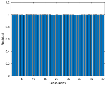
Figure 6: The residual obtained by SCCRC, and the 28th class has the least residual.

From Figs. 2, 4 and 6, we can see that by augmenting the sparsity of coefficients obtained by CCRC, SCCRC can avoid the misclassification scenario to some degree. Next we employ another criteria to illustrate the effectiveness of SCCRC. In wright2009robust , Wright defined a measure of how concentrated the coefficients are on a single class, i.e. sparsity concentration index (SCI), which is defined as,

$$\operatorname{SCI}(\boldsymbol{y})=\frac{C\cdot\underset{i}{\max}\left\|\boldsymbol{\alpha}_{i}\right\|_{1}/\|\boldsymbol{\alpha}\|_{1}-1}{C-1}\in[0,1]$$ (18)

Bigger values of SCI means enhanced sparsity; therefore, we exploit this index to calculate the SCI of the above test sample. The values of SRC, CCRC and our proposed SCCRC are 0.0428, 0.0714 and 0.2079, respectively. We can see that by introducing the competitive regularization term, sparsity of CCRC is improved compared with SRC. By combining sparse and collaborative-competitive representation, our proposed SCCRC achieves the highest sparsity, thus improved classification results can be expected.

4 Experimental results and analysis

In this section, we report the performance of SCCRC on five publicly available datasets, i.e. ORL samaria1994parameterisation , Georgia Tech goel2005face , FERET phillips1997feret , Extended Yale B georghiades2001few and AR databases martinez2007ar . We compare the classification accuracy of SCCRC with SRC wright2009robust , LRC naseem2010linear , CRC zhang2011sparse , SCRC zeng2017multiplication , NRC xu2019sparse , ProCRC cai2016probabilistic CCRC yuan2018collaborative and CCRC-$\ell_{1}$. In addition, we present the classification time (in seconds) of all the competing approaches. We use SolveFISTA.m yang2010fast to solve the sparse optimization problem. The parameters $\lambda_{1}$ and $\lambda_{2}$ in CCRC and our proposed SCCRC are selected from the set $\left\{10^{-7},10^{-6},\cdots,1,10,100\right\}$. All experiments are conducted with MATLAB R2019b under Windows 10 on a PC equipped with Intel i9-8950HK 2.90 GHz CPU and 32 GB RAM.

4.1 Experiments on the ORL database

The ORL database contains 400 images of 40 individuals. For each subject, there are 10 images with the variations in lighting, facial expression and facial details (with or without glasses), Fig. 7 shows some face images from this database. In our experiments, each image is resized to 56$\times$46, and the first 1 to 6 images per person are selected as training samples and the remaining are testing samples.

The recognition accuracy and the testing time (when the first 6 images per subject are used as training samples) of different methods are shown in Table 2. We can see that SCCRC outperforms all the competing approaches in terms of recognition accuracy. Meanwhile, the testing time of SCCRC is comparable to that of SCRC, and it is 31 times faster than NRC. With the increase of the number of training samples, the classification accuracy of SCCRC increases consistently. By integrating SRC and CRC, SCRC obtains better results than those of SRC and CRC, especially when the number of training samples is relatively small. By introducing the non-negative constraint, NRC exhibits superiority over SRC and CRC. Thanks to the competitive regularization term, CCRC outperforms CRC with the increasing number of training samples.

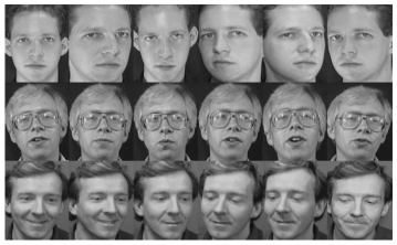
Figure 7: Example images from the ORL database.

Table 2: Classification accuracy (%) and the testing time of competing approaches on the ORL database.

Methods	1	2	3	4	5	6	testing time (s)
SRC wright2009robust	73.06	82.50	84.64	88.33	88.50	92.50	0.79
LRC naseem2010linear	67.50	79.38	81.43	86.25	88.00	94.38	0.70
CRC zhang2011sparse	71.67	83.75	86.07	91.25	90.50	92.50	0.34
SCRC zeng2017multiplication	73.89	86.56	86.43	91.25	92.50	92.50	0.77
NRC xu2019sparse	72.78	87.19	88.21	90.00	90.00	93.75	28.66
ProCRC cai2016probabilistic	67.50	85.00	86.07	90.41	92.00	94.37	0.09
CCRC yuan2018collaborative	68.06	85.63	87.50	90.83	92.50	94.38	0.29
CCRC-$\ell_{1}$	71.67	85.63	87.14	90.00	89.50	93.13	0.29
SCCRC	73.89	87.81	88.57	91.67	93.00	95.00	0.91

4.2 Experiments on the GT database

There are 750 face images (50 individuals and each has 15 images) in the GT face database. These face images show frontal and/or tilted faces with different facial expressions, lighting conditions and scale. In our experiments, all images are cropped and resized to 60$\times$50. Fig. 8 shows some cropped face images from the GT face dataset. The first 1-6 face images of each subject are used as training samples, and the remaining images are regarded as testing samples.

Table 3 lists the classification accuracy and the testing time (when the first 6 images per subject are used as training samples) of compared methods on the GT database. One can see that with the increasing number of training samples, accuracy of all competing methods is increased, and the proposed SCCRC achieves the best results in most cases. Moreover, ProCRC has the shortest testing time, and SCCRC is 25 times faster than NRC.

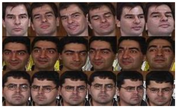
Figure 8: Example images from the GT database.

Table 3: Classification accuracy (%) and the testing time of various approaches on the GT database.

Methods	1	2	3	4	5	6	testing time (s)
SRC wright2009robust	38.71	47.38	49.17	52.18	53.60	62.44	5.38
LRC naseem2010linear	36.14	46.62	51.33	55.64	59.60	67.33	2.81
CRC zhang2011sparse	36.43	46.00	49.33	54.36	58.40	64.67	1.68
SCRC zeng2017multiplication	37.71	48.31	53.83	56.91	61.20	68.00	4.47
NRC xu2019sparse	36.86	47.69	50.33	57.82	60.20	66.89	116.20
ProCRC cai2016probabilistic	34.14	45.69	51.33	55.09	58.40	63.77	0.35
CCRC yuan2018collaborative	33.43	44.46	48.67	51.64	55.40	61.33	1.30
CCRC-$\ell_{1}$	33.86	44.77	48.67	51.64	55.20	62.89	1.32
SCCRC	39.14	50.15	54.50	57.64	62.20	68.89	4.57

4.3 Experiments on the FERET database

This subset used is from the well-known FERET face database, which consists of 1400 face images of 200 subjects, each provided with seven different face images. This subset is composed of images in the original FERET face data set whose names are marked with two-character strings: ba, bj, bk, be, bf, bd, and bg. Fig. 9 shows some of these face images. Each face image is resized to a 40$\times$40 image. The first 1-6 face images of each subject are selected as training samples, and the rest as testing samples.

Table 4 details the classification results of competing methods. One can see that SCCRC is very efficient, and its testing time is only one-fifth of that of NRC. The classification results of all approaches drop when the number of training samples per subject is 3,  zeng2017multiplication also reported this observation. The reason behind this phenomenon is that we select the first 3 images for all subjects, that is, the indices of training samples are fixed across different individuals. A more reasonable way is to randomly choose the training samples for each subject.

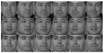
Figure 9: Example images from the FERET database.

Table 4: Classification accuracy (%) and the testing time of different methods on the FERET database.

Methods	1	2	3	4	5	6	testing time (s)
SRC wright2009robust	45.83	57.20	52.38	68.00	76.25	79.50	8.57
LRC naseem2010linear	44.50	63.10	58.88	76.33	81.50	75.50	3.36
CRC zhang2011sparse	40.67	55.60	47.38	56.83	65.25	69.50	12.96
SCRC zeng2017multiplication	45.67	61.90	56.00	69.17	80.50	80.50	8.61
NRC xu2019sparse	46.33	59.90	52.62	63.00	73.75	73.00	42.46
ProCRC cai2016probabilistic	39.75	54.90	42.87	49.66	56.75	50.00	0.43
CCRC yuan2018collaborative	42.08	57.20	48.25	53.83	57.00	47.00	5.59
CCRC-$\ell_{1}$	43.42	58.50	48.63	59.33	69.75	68.50	6.09
SCCRC	47.83	65.50	60.12	74.83	83.25	85.50	8.92

In order to demonstrate the statistical significance of our proposed SCCRC compared with the other methods, we conduct a significance test, McNemar’s test wen2018low ; li2015learning , for the results shown in Table 4. The significance level, i.e., $p$-value is set as 0.05, which means that the performance difference between two methods is statistically significant, if the estimated $p$-value is lower than 0.05. Table 5 lists the $p$-values between SCCRC and the other methods. From this table, one can see that the performance differences between SCCRC and the methods (SRC, CRC, SCRC, ProCRC, CCRC and CCRC-$\ell_{1}$) are statistically significant in all cases. The performance differences between SCCRC and LRC/NRC are not statistically significant; however, SCCRC outperforms NRC in all cases, and SCCRC is superior to LRC except when there are 4 training samples per subject. The above experimental results validate the effectiveness of our proposed SCCRC.

Table 5: $p$-value between SCCRC and the other methods on the FERET database. $*$ indicates that the difference between the two methods is statistically significant when $p$=0.05.

Methods	1	2	3	4	5	6
SRC wright2009robust	$0.0165^{*}$	6.59$\times 10^{-12*}$	2.54$\times 10^{-8*}$	2.73$\times 10^{-6*}$	2.64$\times 10^{-4*}$	$0.0146^{*}$
LRC naseem2010linear	$0.0011^{*}$	$0.0399^{*}$	0.3291	0.2370	0.3222	1.03$\times 10^{-4*}$
CRC zhang2011sparse	3.90$\times 10^{-9*}$	1.05$\times 10^{-14*}$	1.83$\times 10^{-16*}$	5.67$\times 10^{-18*}$	2.52$\times 10^{-16*}$	1.02$\times 10^{-7*}$
SCRC zeng2017multiplication	$0.0271^{*}$	2.18$\times 10^{-4*}$	3.74$\times 10^{-4*}$	7.27$\times 10^{-4*}$	$0.0227^{*}$	$0.0127^{*}$
NRC xu2019sparse	0.1783	6.71$\times 10^{-7*}$	5.68$\times 10^{-8*}$	1.13$\times 10^{-8*}$	4.00$\times 10^{-8*}$	8.67$\times 10^{-7*}$
ProCRC cai2016probabilistic	1.79$\times 10^{-10*}$	6.32$\times 10^{-16*}$	1.28$\times 10^{-23*}$	1.46$\times 10^{-26*}$	2.58$\times 10^{-23*}$	5.23$\times 10^{-19*}$
CCRC yuan2018collaborative	5.55$\times 10^{-6*}$	2.93$\times 10^{-10*}$	2.74$\times 10^{-13*}$	4.65$\times 10^{-19*}$	2.20$\times 10^{-21*}$	1.02$\times 10^{-20*}$
CCRC-$\ell_{1}$	1.77$\times 10^{-4*}$	1.32$\times 10^{-8*}$	5.26$\times 10^{-14*}$	1.70$\times 10^{-12*}$	1.49$\times 10^{-12*}$	3.62$\times 10^{-7*}$

4.4 Experiments on the Extended Yale B database

The Extended Yale B georghiades2001few face dataset contains 2414 frontal facial images of 38 individuals. These images are captured under various controlled lighting conditions. The size of an image is 192$\times$168 pixels. In our experiments, all images are cropped and resized to 32$\times$32 pixels. Fig. 10 shows some face images from the Extended Yale B face dataset. The first 5, 10, 15, 20, 25 and 30 face images of each subject are treated as training samples and the remaining as testing samples.

Classification accuracy and the testing time (when the first 30 images per subject are used as training samples) of different approaches on this database is listed in Table 6. We can observe that the testing time of SCCRC is comparable to that of SCRC, and it is about 3 times faster than NRC. Similar to the experimental results on the above three databases, classification accuracy of SCCRC increases steadily with the increasing number of training samples per subject, and the performance gain is significant when the number of training samples is increasing. For example, when the number of training samples is 15, SCCRC has more than 6.73% higher accuracy than the second best method, i.e., LRC.

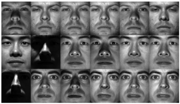
Figure 10: Example images from the Extended Yale B database.

Table 6: Classification accuracy (%) and the testing time of competing algorithms on the Extended Yale B database.

Methods	5	10	15	20	25	30	testing time (s)
SRC wright2009robust	40.51	41.79	38.77	41.17	44.81	44.82	38.82
LRC naseem2010linear	46.27	75.22	75.27	76.06	83.06	85.01	14.69
CRC zhang2011sparse	48.29	68.24	74.13	77.81	79.85	85.09	5.45
SCRC zeng2017multiplication	46.09	57.03	65.94	69.11	67.62	71.82	41.59
NRC xu2019sparse	51.08	65.93	71.04	74.12	77.12	81.63	113.94
ProCRC cai2016probabilistic	52.02	69.27	73.69	77.14	80.94	85.63	0.36
CCRC yuan2018collaborative	54.99	72.62	74.95	77.33	83.06	85.56	2.54
CCRC-$\ell_{1}$	51.89	71.14	75.05	78.66	85.25	89.80	5.86
SCCRC	52.97	79.25	82.00	83.56	83.81	87.21	40.41

4.5 Experiments on the AR database

AR database includes over 4000 face images of 126 people (70 male and 56 female) which vary in expression, illumination and disguise (wearing sunglasses or scarves). Each subject has 26 images consisting of 14 clean images, 6 images with sunglasses and 6 images with scarves. As in jiang2013label ; yuan2018collaborative , we use a subset that contains 1400 clean faces selected from 50 male and 50 female subjects, all the images are resized to 28$\times$20, and some example images are shown in Fig. 11. For each subject, we use the first 1-6 face images as training samples, and the remaining as testing samples. Experimental results are shown in Table 7. Once again, SCCRC outperforms the other competing approaches in terms of classification accuracy except for the case of 2 training samples per person.

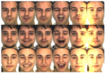
Figure 11: Example images from the AR database.

Table 7: Classification accuracy (%) and the testing time of evaluating methods on the AR database.

Methods	1	2	3	4	5	6	testing time (s)
SRC wright2009robust	59.00	56.33	53.91	52.90	55.67	61.12	4.19
LRC naseem2010linear	58.08	56.92	55.64	56.50	60.00	75.50	5.06
CRC zhang2011sparse	58.15	60.42	61.09	65.70	76.89	91.50	2.91
SCRC zeng2017multiplication	62.08	64.17	65.00	66.70	75.78	88.62	4.48
NRC xu2019sparse	65.31	68.33	68.64	72.60	84.00	93.00	17.41
ProCRC cai2016probabilistic	68.46	73.00	75.72	75.70	84.00	91.62	0.28
CCRC yuan2018collaborative	67.62	71.92	72.82	73.20	83.00	91.25	1.17
CCRC-$\ell_{1}$	63.77	68.75	70.36	73.30	85.11	93.13	1.49
SCCRC	70.00	72.75	77.27	78.90	86.11	93.63	4.54

4.6 Experiments on the corrupted face images

To explore the robustness of our proposed method to noise, we use corrupted face images as test data. Here the AR database is used for evaluation, as in Section 4.5, 1400 images of 100 subjects are selected, and the size of image is 28$\times$20. The first seven images are used as training samples and the remaining as test samples. We add zero-mean, Gaussian white noise with variance of 0.01 to all the test images, some corrupted test face images are shown in Fig. 12. Experimental results of all competing approaches are shown in Table 8. It can be seen that by introducing the $\ell_{1}$-norm constraint on the coefficient vector, CCRC-$\ell_{1}$ outperforms CCRC by 10.14%. Our proposed SCCRC achieves the highest accuracy, and it is around 2.4 times faster than NRC.

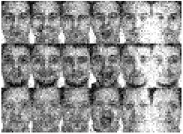
Figure 12: Some corrupted test images from the AR database.

Table 8: Classification accuracy and the testing time of evaluating methods on the corrupted face images.

Methods	Accuracy (%)	testing time (s)
SRC wright2009robust	84.57	10.82
LRC naseem2010linear	74.57	4.75
CRC zhang2011sparse	82.14	2.80
SCRC zeng2017multiplication	84.00	4.84
NRC xu2019sparse	86.14	26.85
ProCRC cai2016probabilistic	83.14	0.29
CCRC yuan2018collaborative	75.00	1.25
CCRC-$\ell_{1}$	85.14	1.65
SCCRC	87.29	11.27

4.7 Experiment analysis

The classification results on five databases validate the effectiveness and robustness of our proposed SCCRC. Based on the experimental results on these databases, the following observations can be made:

(1) By enhancing the sparsity of representation of CRC, SCRC outperforms SRC and CRC in most cases, which reveals that sparseness of collaborative representation explicitly contributes to accurate classification of test samples.

(2) Thanks to the non-negative constraint on the coefficient vector, NRC achieves higher classification accuracy than SRC and CRC, which demonstrates the discriminative capability of the non-negative regularization term.

(3) By introducing the competitive representation term, CCRC is superior to CRC in terms of classification accuracy. This regularization term promotes competitive representation between distinct classes, which encourages the coefficient vector to be sparse to some extent.

(4) On the clean test images, improvement of CCRC-$\ell_{1}$ over CCRC is not that significant. However, on the corrupted test images, CCRC-$\ell_{1}$ outperforms CCRC by 10.14%, which again verifies that sparsity of coefficient vector is necessary to improve the classification performance.

(5) Both on the clean and corrupted test images, our proposed SCCRC performs the best, which indicates that SCCRC needs clean training images. Like conventional RBCM, our proposed SCCRC is a general classification framework and it can be applied in other pattern classification tasks. For corrupted training images, as in iliadis2017robust , we can first employ low rank matrix recovery techniques (e.g., robust PCA candes2011robust and its variants) to obtain clean training images, then SCCRC can be used for classification.

4.8 Parameter sensitiveness analysis

In our proposed SCCRC, there are three parameters to be determined, i.e. one parameter $\lambda$ for SRC and two parameters $\lambda_{1}$ and $\lambda_{2}$ for CCRC. We set $\lambda$=0.001 for SRC as in SCRC. To examine how the remaining parameters $\lambda_{1}$ and $\lambda_{2}$ influence the performance of SCCRC, we conduct experiments on the AR database. Experimental setting is the same as in Section 4.5 and the number of training samples per subject is 6. Fig. 13 illustrates the effect of parameter selection. We can see that SCCRC achieves superb results when both $\lambda_{1}$ and $\lambda_{2}$ are in proper range. More specifically, the performance is better when $\lambda_{2}$ is in the range of [0.0001 0.001], which validates the necessity of the competitive term in CCRC. Similarly, SCCRC can achieve better results when $\lambda_{1}$ is in the range of [0.0001 0.001]. To better illustrate the influence of $\lambda_{1}$ and $\lambda_{2}$, we plot the recognition accuracy against the variation of one parameter when the other is fixed. Fig. 14 shows the influence of $\lambda_{2}$ when $\lambda_{1}$=0.001, we can see that the performance of SCCRC is desirable when $\lambda_{2}$ is assigned to a small value. Fig. 15 presents the effect of $\lambda_{1}$ when $\lambda_{2}$=0.001, one can see that SCCRC performs stable when $\lambda_{1}$ is in the range of [0.0001 0.01]. Based on the above experimental results, we set $\lambda_{1}$=0.001 and $\lambda_{2}$=0.001 on the AR database.

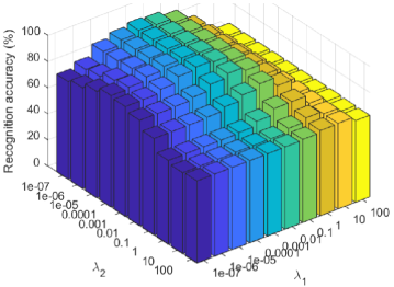
Figure 13: Recognition accuracy of SCCRC versus parameters $\lambda_{1}$ and $\lambda_{2}$ on the AR database.

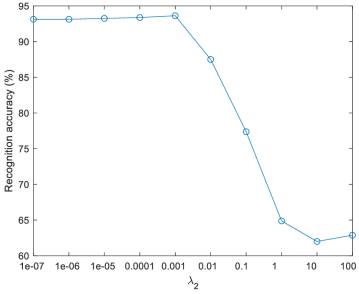
Figure 14: Recognition accuracy versus the variation of parameter $\lambda_{2}$ when $\lambda_{1}$=0.001.

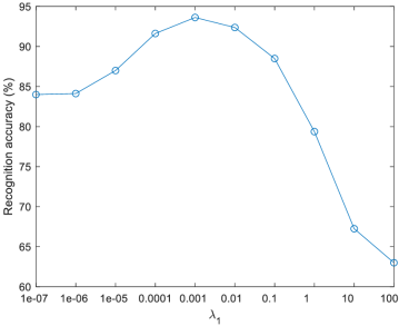
Figure 15: Recognition accuracy versus the variation of parameter $\lambda_{1}$ when $\lambda_{2}$=0.001.

5 Conclusions

Sparse representation based classification (SRC) and collaborative representation based classification (CRC) have been widely studied due to their promising results for classification. Although CRC reveals that it is the collaborative representation mechanism rather than the $\ell_{1}$-norm sparsity that makes SRC powerful, sparsity should not be completely ignored. Thus, in this paper, we propose a new technique to enhance the sparsity of CCRC by multiplying the coefficients of SRC and CCRC. Experiments on five publicly available databases validate the effectiveness of our proposed SCCRC, and demonstrate that SCCRC outperforms other representation based classification approaches.

In this paper, we did not explicitly consider the situation that both the training and test samples are contaminated due to occlusion or corruption, thus in future, we will extend SCCRC to tackle the above scenarios.

- (1) X. Qu, W. Wang, K. Lu, J. Zhou, In-air handwritten chinese character recognition with locality-sensitive sparse representation toward optimized prototype classifier, Pattern Recognition 78, 267 (2018)
- (2) R. Prates, W.R. Schwartz, Kernel cross-view collaborative representation based classification for person re-identification, Journal of Visual Communication and Image Representation 58, 304 (2019)
- (3) J. Yang, J. Qian, Hyperspectral image classification via multiscale joint collaborative representation with locally adaptive dictionary, IEEE Geoscience and Remote Sensing Letters 15(1), 112 (2018)
- (4) J. Wright, A.Y. Yang, A. Ganesh, S.S. Sastry, Y. Ma, Robust face recognition via sparse representation, IEEE transactions on pattern analysis and machine intelligence 31(2), 210 (2009)
- (5) C.G. Li, J. Guo, H.G. Zhang, in 2010 20th International Conference on Pattern Recognition (IEEE, 2010), pp. 649–652
- (6) N. Zhang, J. Yang, in 2010 Chinese conference on pattern recognition (CCPR) (IEEE, 2010), pp. 1–5
- (7) E.G. Ortiz, B.C. Becker, Face recognition for web-scale datasets, Computer Vision and Image Understanding 118, 153 (2014)
- (8) M. Aharon, M. Elad, A. Bruckstein, et al., K-svd: An algorithm for designing overcomplete dictionaries for sparse representation, IEEE Transactions on signal processing 54(11), 4311 (2006)
- (9) Q. Zhang, B. Li, in 2010 IEEE Computer Society Conference on Computer Vision and Pattern Recognition (IEEE, 2010), pp. 2691–2698
- (10) Z. Jiang, Z. Lin, L.S. Davis, Label consistent k-svd: Learning a discriminative dictionary for recognition, IEEE transactions on pattern analysis and machine intelligence 35(11), 2651 (2013)
- (11) I. Kviatkovsky, M. Gabel, E. Rivlin, I. Shimshoni, On the equivalence of the lc-ksvd and the d-ksvd algorithms, IEEE transactions on pattern analysis and machine intelligence 39(2), 411 (2017)
- (12) Y. Song, Y. Liu, Q. Gao, X. Gao, F. Nie, R. Cui, Euler label consistent k-svd for image classification and action recognition, Neurocomputing 310, 277 (2018)
- (13) L. Zhang, M. Yang, X. Feng, in 2011 International conference on computer vision (IEEE, 2011), pp. 471–478
- (14) Y. Xu, Z. Zhong, J. Yang, J. You, D. Zhang, A new discriminative sparse representation method for robust face recognition via {} regularization, IEEE transactions on neural networks and learning systems 28(10), 2233 (2017)
- (15) S. Zeng, J. Gou, L. Deng, An antinoise sparse representation method for robust face recognition via joint l1 and l2 regularization, Expert Systems with Applications 82, 1 (2017)
- (16) S. Cai, L. Zhang, W. Zuo, X. Feng, in Proceedings of the IEEE conference on computer vision and pattern recognition (2016), pp. 2950–2959
- (17) R. Lan, Y. Zhou, Z. Liu, X. Luo, Prior knowledge-based probabilistic collaborative representation for visual recognition, IEEE transactions on cybernetics (2018)
- (18) H. Yuan, X. Li, F. Xu, Y. Wang, L.L. Lai, Y.Y. Tang, A collaborative-competitive representation based classifier model, Neurocomputing 275, 627 (2018)
- (19) C. Zheng, N. Wang, Collaborative representation with k-nearest classes for classification, Pattern Recognition Letters 117, 30 (2019)
- (20) J. Waqas, Z. Yi, L. Zhang, Collaborative neighbor representation based classification using l2-minimization approach, Pattern Recognition Letters 34(2), 201 (2013)
- (21) J. Gou, L. Wang, Z. Yi, J. Lv, Q. Mao, Y.H. Yuan, A new discriminative collaborative neighbor representation method for robust face recognition, IEEE Access 6, 74713 (2018)
- (22) N. Akhtar, F. Shafait, A. Mian, Efficient classification with sparsity augmented collaborative representation, Pattern Recognition 65, 136 (2017)
- (23) S. Zeng, X. Yang, J. Gou, Multiplication fusion of sparse and collaborative representation for robust face recognition, Multimedia Tools and Applications 76(20), 20889 (2017)
- (24) W. Li, Q. Du, F. Zhang, W. Hu, Hyperspectral image classification by fusing collaborative and sparse representations, IEEE Journal of Selected Topics in Applied Earth Observations and Remote Sensing 9(9), 4178 (2016)
- (25) J. Xu, W. An, L. Zhang, D. Zhang, Sparse, collaborative, or nonnegative representation: Which helps pattern classification?, Pattern Recognition 88, 679 (2019)
- (26) I. Naseem, R. Togneri, M. Bennamoun, Linear regression for face recognition, IEEE transactions on pattern analysis and machine intelligence 32(11), 2106 (2010)
- (27) W. Deng, J. Hu, J. Guo, in Proceedings of the IEEE conference on computer vision and pattern recognition (2013), pp. 399–406
- (28) W. Deng, J. Hu, J. Guo, Face recognition via collaborative representation: Its discriminant nature and superposed representation, IEEE transactions on pattern analysis and machine intelligence 40(10), 2513 (2018)
- (29) P.L. Combettes, V.R. Wajs, Signal recovery by proximal forward-backward splitting, Multiscale Modeling & Simulation 4(4), 1168 (2005)
- (30) F.S. Samaria, A.C. Harter, in Proceedings of 1994 IEEE Workshop on Applications of Computer Vision (IEEE, 1994), pp. 138–142
- (31) N. Goel, G. Bebis, A. Nefian, in Biometric Technology for Human Identification II, vol. 5779 (International Society for Optics and Photonics, 2005), vol. 5779, pp. 426–438
- (32) P.J. Phillips, H. Moon, P. Rauss, S.A. Rizvi, in Proceedings of IEEE Computer Society Conference on Computer Vision and Pattern Recognition (IEEE, 1997), pp. 137–143
- (33) A.S. Georghiades, P.N. Belhumeur, D.J. Kriegman, From few to many: Illumination cone models for face recognition under variable lighting and pose, IEEE Transactions on Pattern Analysis & Machine Intelligence (6), 643 (2001)
- (34) A. Martínez, R. Benavente, The ar face database, Computer Vision Center, Technical Report 24 (1998)
- (35) A.Y. Yang, S.S. Sastry, A. Ganesh, Y. Ma, in 2010 IEEE International Conference on Image Processing (IEEE, 2010), pp. 1849–1852
- (36) J. Wen, X. Fang, Y. Xu, C. Tian, L. Fei, Low-rank representation with adaptive graph regularization, Neural Networks 108, 83 (2018)
- (37) S. Li, Y. Fu, Learning robust and discriminative subspace with low-rank constraints, IEEE transactions on neural networks and learning systems 27(11), 2160 (2015)
- (38) M. Iliadis, H. Wang, R. Molina, A.K. Katsaggelos, Robust and low-rank representation for fast face identification with occlusions, IEEE Transactions on Image Processing 26(5), 2203 (2017)
- (39) E.J. Candès, X. Li, Y. Ma, J. Wright, Robust principal component analysis?, Journal of the ACM (JACM) 58(3), 11 (2011)