Introduction to molecular dynamics simulations

Abstract

We provide an introduction to molecular dynamics simulations in the context of the Kob-Andersen model of a glass. We introduce a complete set of tools for doing and analyzing the results of simulations at fixed NVE and NVT. The modular format of the paper allows readers to select sections that meet their needs. We start with an introduction to molecular dynamics independent of the programming language, followed by introductions to an implementation using Python and then the freely available open source software package LAMMPS. We also describe analysis tools for the quick testing of the program during its development and compute the radial distribution function and the mean square displacement using both Python and LAMMPS.

I Introduction

Computer simulations are a powerful approach for addressing questions which are not accessible by theory and experiments. Simulations give us access to analytically unsolvable systems, and contrary to laboratory experiments, there are no unknown “impurities” and we can work with a well defined model. In this paper we focus on the simulation of many particle systems using molecular dynamics, which models a system of classical particles whose dynamics is described by Newton’s equations and its generalizations.

Our goal is to provide the background for those who wish to use and analyze molecular dynamics simulations. This paper may also be used in a computer simulation course or for student projects as part of a course.

Many research groups no longer write their own molecular dynamics programs, but use instead highly optimized and complex software packages such as LAMMPS.LAMMPSwebpage To understand the core of these software packages and how to use them wisely, it is educational for students to write and use their own program before continuing with a software package. One intention of this paper is to guide students through an example of a molecular dynamics simulation and then implement the same task with LAMMPS. A few examples are given to illustrate the wide variety of possibilities for analyzing molecular dynamics simulations and hopefully to lure students into investigating the beauty of many particle systems.

Although we discuss the Python programming language, the necessary tools are independent of the programming language and are introduced in Sec. II. Those who prefer to start programming with minimal theoretical background may start with Sec. III and follow the guidance provided on which subsection of Sec. II is important for understanding the corresponding subsection in Sec. III.

Throughout the paper we refer to problems that are listed in Sec. VII. Answers to Problems (1)–(9) are given in the text immediately following their reference. These suggested problems are intended to encourage active engagement with the paper by encouraging readers to work out sections of the paper by themselves.

II Molecular Dynamics Simulation

II.1 Introduction

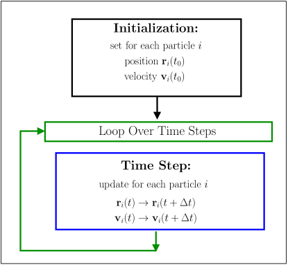
Figure 1: Flow chart of a molecular dynamics simulation program.

Molecular dynamics simulates a classical system of $N$ particles. The core of most simulations is to start with the initial positions and velocities of all particles and to then repeatedly apply a “recipe” to update each particle’s position and velocity from time $t$ to time $t+\Delta t$ (see Fig. 1). The dynamics is governed by Newton’s second law

$$\mathbf{F}_{i}=m_{i}\mathbf{a}_{i},$$ (1)

where $\mathbf{a}_{i}$ is the acceleration of particle $i$.

In Sec. II.2 we define the net force $\mathbf{F}_{i}$ which is used in this paper and discuss in Sec. II.4 the update rules for the positions $\mathbf{r}_{i}$ and velocities $\mathbf{v}_{i}$.

II.2 Model

The model is specified by the net force $\mathbf{F}_{i}$ on each particle of mass $m_{i}$. The force $\mathbf{F}_{i}$ can be due to all other particles and/or additional interactions such as effective drag forces or interactions with a wall or an external field. In the following we will consider only conservative forces which are due to all the other particles. We also assume pair-wise interactions given by a potential

$$V=\sum\limits_{i=1}^{N-1}\sum\limits_{j=i+1}^{N}V_{ij}.$$ (2)

Specifically, we use the Lennard-Jones potential

$$V_{ij}=4\epsilon\left[\left(\frac{\sigma}{r_{ij}}\right)^{12}-\left(\frac{\sigma}{r_{ij}}\right)^{6}\right],$$ (3)

where $r_{ij}=|\mathbf{r}_{i}-\mathbf{r}_{j}|$ is the distance between particle $i$ at position $\mathbf{r}_{i}$ and particle $j$ at position $\mathbf{r}_{j}$.

The advantage of the Lennard-Jones potential is that it can be used to simulate a large variety of systems and scenarios. For example, each particle may represent an atom, a colloid, or a monomer of a polymer. woodParker1957 ; kobAndersenPRL1994 ; guzmanDePablo2003 ; bennemann1998 Depending on parameters such as the temperature, density, and shear stress the particles may form a gas, liquid, or solid (crystal or glass).HansenVerlet1969 ; abramo2015 ; kobAndersenPRL1994 The reason for this wide variety of applications is that the Lennard-Jones potential incorporates two major effective forces: a strong repulsive force for short distances and an attractive force for intermediate distances. The attractive term of the Lennard-Jones potential $\propto(\sigma/r)^{6}$ is the van der Waals interaction due to mutual polarization of two particles. HansenMcDonald The repulsive part $\propto(\sigma/r)^{12}$ is proportional to a power of $(\sigma/r)^{6}$ and thus simplifies the computation of the force. Note that the Lennard-Jones potential is short-range. For long-range interactions (gravitational and Coulomb) more advanced techniques are necessary.allen90 See Refs. allen90, ; rapaport98, ; HansenMcDonald, for an overview of further applications of the Lennard-Jones potential and other particle interactions and additional contributions to $\mathbf{F}$.

In this paper we illustrate how to simulate a glass forming system. We use the binary Kob-Anderson potential, kobAndersenPRL1994 ; kobAndersenPRE51_1995 ; kobAndersenPRE52_1995 which has been developed as a model for the Ni₈₀P₂₀ alloy,kobAndersenPRE51_1995 and has become one of the major models for studying supercooled liquids, glasses, and crystallization. Examples are discussed in Refs. kobAndersenPRL1994, ; kobAndersenPRE51_1995, ; kobAndersenPRE52_1995, ; KVLKobBinder_1996, ; hassani2016, ; schoenholz2016, ; ShrivastavPRE2016, ; makeevPriezjev2018, ; pedersenSchroederDyrePRL_2018, and references cited in Refs. kobAndersenPRL1994, ; makeevPriezjev2018, ; pedersenSchroederDyrePRL_2018, . The Kob-Andersen model is an 80:20 mixture of particles of type $A$ and $B$. The Lennard-Jones potential in Eq. (3) is modified by the dependence of $\epsilon$ and $\sigma$ on the particle type $\alpha,\beta\in\{A,B\}$ of particles $i$ and $j$.

$$V_{ij}=V_{\alpha\beta}(r_{ij})=4\epsilon_{\alpha\beta}\left[\left(\frac{\sigma_{\alpha\beta}}{r_{ij}}\right)^{12}-\left(\frac{\sigma_{\alpha\beta}}{r_{ij}}\right)^{6}\right].$$ (4)

We use units such that $\sigma_{AA}=1$ (length unit), $\epsilon_{AA}=1$ (energy unit), $m_{A}=1$ (mass unit), and $k_{\rm B}=1$ (the temperature unit is $\epsilon_{AA}/k_{\rm B}$). The resulting time unit is $\sqrt{m_{A}\sigma_{AA}^{2}/\epsilon_{AA}}$. With these units, the Kob-Andersen parameters are $\sigma_{AA}=1.0$, $\epsilon_{AA}=1.0$, $\sigma_{AB}=0.8$, $\epsilon_{AB}=1.5$, $\sigma_{BB}=0.88$, $\epsilon_{BB}=0.5$, and $m_{A}=m_{B}=1.0$. To save computer time, the potential is truncated and shifted at $r_{ij}=r^{\rm cut}_{\alpha\beta}=2.5\,\sigma_{\alpha\beta}$

$$V_{ij}^{\rm cutoff}=\begin{cases}V_{\alpha\beta}(r_{ij})-V_{\alpha\beta}(r^{\rm cut}_{\alpha\beta})&\mbox{$r_{ij}<r^{\rm cut}_{\alpha\beta}$}\\ 0&\mbox{(otherwise)}.\end{cases}$$ (5)

For the truncated and shifted KA-LJ system, $V$ is given by Eq. (2) by replacing $V_{ij}$ with $V_{ij}^{\rm cutoff}$.

The force is given by $\mathbf{F}_{i}=-\nabla_{i}V$. The $x$-component of the force on particle $i$ is given by (see Problem 1)

$$F_{i,x}=48\sum_{{\rm neighbors}\,j}\epsilon_{\alpha\beta}\left(\frac{\sigma_{\alpha\beta}^{12}}{r_{ij}^{14}}-0.5\frac{\sigma_{\alpha\beta}^{6}}{r_{ij}^{8}}\right)(x_{i}-x_{j}).$$ (6)

and similarly for $F_{i,y}$ and $F_{i,z}$. The sum is only over particles $j$ for which $j\neq i$ and $r_{ij}<2.5\,\sigma_{\alpha\beta}$.

II.3 Periodic boundary conditions and the minimum image convention

To determine the neighbors we need to specify the boundaries of the system. We will assume that the goal of the simulation is to model the structure and dynamics of particles in a very large system ($N\approx 10^{23}$) far from the boundaries. However, most molecular dynamics simulations contain on the order of $10^{3}$–$10^{6}$ particles. To minimize the effect of the boundaries, we use periodic boundary conditions as illustrated in Fig. 2 for a two-dimensional system of linear dimension $L$. The system, framed by thick lines, is assumed to be surrounded by periodic images (framed by thin lines). For particle $i$ the neighboring particles within a distance $r^{\rm cut}_{\alpha\beta}$ are the particles inside the (blue) large circle. To determine the distance $r_{ij}$ between particles $i$ and $j$, we use the “minimum image convention.” For example, the distance between $i$ and particle $j=18$ would be $r_{ij}>r^{\rm cut}_{\alpha\beta}$ without using periodic images because particle 18 in the left bottom corner of the system is outside the (blue) large circle. But with periodic images $r_{ij}<r^{\rm cut}_{\alpha\beta}$ because the nearest periodic image of particle 18 is above particle $i$ within the blue circle. For particles $i$ and $j=20$ we use the direct distance between the two particles within the system (thick frame), because this distance is less than the distance to any of the periodic images of $j=20$.

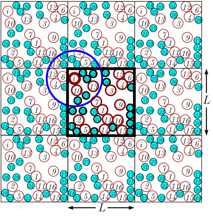
Figure 2: Sketch of a binary two-dimensional system illustrating periodic boundary conditions and the minimum image convention. To identify the neighbors $j$ of particle $i$, the position $\mathbf{r}_{j}$ of particle $j$ is chosen from the position of $j$ within the system (within thick frame) and the positions of $j$’s periodic images (within boxes framed with thin lines), such that $r_{ij}$ is a minimum. Neighbors of $i$ satisfy $r_{ij}<r^{\rm cut}_{\alpha\beta}$ and are within the blue large circle.

II.4 Numerical integration

We next specify the core of a molecular dynamics program, that is, the numerical integration of the $d\times N$ coupled differential equations represented by Eq. (1) (see Fig. 1). We will use the velocity Verlet algorithm

$$\mathbf{r}_{i}\left(t+\Delta t\right) =\mathbf{r}_{i}(t)+\mathbf{v}_{i}(t)\Delta t+\frac{1}{2}\mathbf{a}_{i}(t)\left(\Delta t\right)^{2}$$ (7)

$$\mathbf{v}_{i}\left(t+\Delta t\right) =\mathbf{v}_{i}(t)+\frac{1}{2}[\mathbf{a}_{i}(t)+\mathbf{a}_{i}\left(t+\Delta t\right)]\Delta t.$$ (8)

The velocity Verlet algorithm is commonly used because it is energy drift free and second order in the velocity and third order in the position.gouldTobochnikChristian2007 ; allen90 For other numerical integration techniques we refer readers to Refs. gouldTobochnikChristian2007, ; allen90, ; newman2013, ; numrecipes, . Note that the velocity update in Eq. (8) is directly applicable only if $\mathbf{a}_{i}(t+\Delta t)$ does not depend on $\mathbf{v}_{i}(t+\Delta t)$; that is, $a_{i}(t)$ depends only on the positions of the particles.

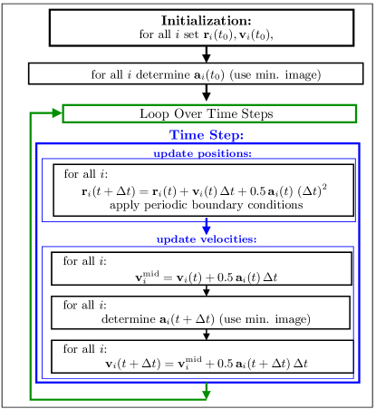
Figure 3: Flow chart for molecular dynamics with the velocity Verlet algorithm.

By using Eqs. (7) and (8) we obtain the flow chart (see Problem 2) in Fig. 3. Most of the computational time is used to determine the accelerations. Note that for each time step $\Delta t$ the accelerations need to be determined only once for $\mathbf{a}_{i}(t+\Delta t)$ (instead of twice for $\mathbf{a}_{i}(t)$ and $\mathbf{a}_{i}(t+\Delta t)$). Thus, only one array for the accelerations is needed, but one must have the correct order of updates within the time step.

II.5 Temperature bath

So far we have used Newton’s second law, Eq. (1), and numerical integration to determine the dynamics, which corresponds to simulating a system at constant energy. We also assumed that the number of particles and the volume are constant, and therefore we have described the NVE or microcanonical ensemble.schroeder2000 ; blundells ; gouldTobochnikStatMech In experiments the temperature $T$ and the pressure $P$ are controlled rather than $E$ and $V$. Many algorithms have been developed for NVT and NPT simulations, including generalizations which allow box shapes to vary during the simulation. For an overview of these algorithms we recommend Refs. allen90, ; gouldTobochnikChristian2007, ; martynaMolPhys1996, . In this section we focus on fixed NVT. We discuss in Sec. II.5.1 an algorithm that also can be used to obtain the initial velocities and then discuss in Sec. II.5.2 the Nosé-Hoover algorithm. A generalization of the latter is the default NVT algorithm in LAMMPS and is used in Sec. IV.3.

II.5.1 Statistical temperature bath

The canonical ensemble corresponds to a system that can exchange energy with a very large system at constant temperature $T$. In equilibrium the probability of a microstate $s$ is proportional to the Boltzmann factor

$$P(s)\propto\mathrm{e}^{-E(s)/k_{\rm B}T},$$ (9)

where $k_{\rm B}$ is Boltzmann’s constant.schroeder2000 ; blundells ; gouldTobochnikStatMech Equation (9) applies to any system. The microstate $s$ is specified by the position and velocity of each particle, $\{\mathbf{r}_{i},\mathbf{v}_{i}\}$, and the system energy is

$$E\left(\{\mathbf{r}_{i},\mathbf{v}_{i}\}\right)=\frac{1}{2}\sum\limits_{i=1}^{N}m_{i}\mathbf{v}_{i}^{2}+V(\{\mathbf{r}_{i}\}).$$ (10)

From Eqs. (9) and (10) it follows that the probability distribution for the $x$-component of the velocity of particle $i$ is given by the Maxwell-Boltzmann distribution

$$P\left(v_{i,x}\right)=\frac{1}{\sqrt{2\pi}\sigma_{i}}\mathrm{e}^{-v_{i,x}^{2}/2\sigma_{i}^{2}},$$ (11)

with the standard deviation

$$\sigma_{i}=\sqrt{\frac{k_{\rm B}T}{m_{i}}}.$$ (12)

The probability distributions for the $y$- and $z$-components of the velocity are obtained by replacing in Eq. (11) $v_{i,x}$ by $v_{i,y}$ and $v_{i,z}$, respectively. schroeder2000 ; blundells ; gouldTobochnikStatMech It is straightforward to show that (see Problem 3)

$$\left\langle E_{\rm kin}\right\rangle=\left\langle\sum\limits_{i=1}^{N}\frac{1}{2}m_{i}v_{i}^{2}\right\rangle=\frac{3N}{2}k_{\rm B}T.$$ (13)

To achieve simulations at fixed NVT Andersenandersen1980 incorporated particle collisions with a temperature bath by choosing the particle velocities from the Maxwell-Boltzmann distribution.allen90 ; gouldTobochnikChristian2007 We will use a slight modification to the Andersen algorithm introduced by Andrea et al.andrea At periodic intervals (approximately every $50$ time steps) all velocities are newly assigned by giving each particle a velocity component $v_{\mu}$ ($\mu\in\{x,y,z\}$) chosen from the Maxwell-Boltzmann distribution in Eqs. (11) and (12).allen90

Figure 4: Flow chart for computing the velocities from the Maxwell-Boltzmann distribution.

Figure 4 shows the flow chart for creating a Maxwell-Boltzmann distribution for the velocities of the particles. Step 1 can be done in any programming language with either already defined functions (see Sec. III.3 for Python and Sec. IV.2 for LAMMPS) or with functions (or subroutines), from for example, Ref. numrecipes, . Step 2 can be skipped when $m_{i}$ is the same for all particles. Step 3 ensures that the center of mass of the system does not drift, and step 4 rescales all the velocities to achieve the desired temperature.

The computer code illustrated by the flow chart of Fig. 4 is inserted into the code described by the flow chart of Fig. 3 with a conditional statement (e.g., if) after the (blue) “Time Step” box and within the (green) “Loop Over Time Steps.” We can also apply steps 1—4 to set the initial velocities $\{\mathbf{v}_{i}(t_{0})\}$ as part of the “Initialization” box in Fig. 3.

II.5.2 Nosé-Hoover algorithm

Another way to implement a constant temperature bath, which is used in LAMMPS,LAMMPSfixnvtp is given by the Nosé-Hoover style algorithm. The key concept for most of the advanced algorithms is that we no longer use Newton’s second law for the equations of motion, but instead use an “extended system” with additional parameters. For the Nosé-Hoover algorithmnosehoover Eq. (1) is replaced by

$$\ddot{\mathbf{r}}_{i} =\frac{{\mathbf{F}}_{i}}{m_{i}}-\xi\,\dot{\mathbf{r}}_{i},$$ (14)

$$\frac{{\rm d}^{2}\ln s}{{\rm d}t^{2}}=\dot{\xi} =\frac{1}{Q}\left(\sum\limits_{i=1}^{N}m_{i}\dot{{\mathbf{r}}}_{i}^{2}-dNk_{\rm B}T\right),$$ (15)

where $d$ is the spatial dimension. The idea is to introduce a fictitious dynamical variable $\xi$ that plays the role of a friction which changes the acceleration until the temperature equals the desired value. The parameter $Q$ is the mass of the temperature bath. Equations (14) and (15) follow from generalizations of Hamiltonian mechanicsTaylor and can be written as first-order differential equations for $\dot{\mathbf{r}}_{i}$, $\dot{\mathbf{p}}_{i}$, and $\dot{\xi}$. nosehoover ; Frenkel2002 ; nose1984 ; branka ; martynaJCP1994 ; martynaMolPhys1996 ; tuckerman2001 A simplified derivation of these equations is given in Appendix A for readers who are familiar with Hamiltonian mechanics.

A generalization of Eqs. (14) and (15) is the Nosé-Hoover chain method, which includes variables for several temperature baths, corresponding to more accurate dynamics in cases with more constraints than the example presented in this paper. shinoda2004 ; martynaKleinTuckermanJCP1992 ; martynaMolPhys1996 ; martynaJCP1994 ; Frenkel2002

Given the equations of motion, our task is to convert them to appropriate difference equations so that we can use numerical integration. We would like to use the velocity Verlet algorithm in Eqs. (7) and (8). However, Eq. (14) for $\mathbf{a}_{i}$ depends on the velocity $\dot{\mathbf{r}}_{i}$, which means that the right side of Eq. (8) also depends on $\mathbf{v}_{i}(t+\Delta t)$. Fox and Andersen fox suggested a velocity-Verlet numerical integration technique that can be applied when the equations of motion are of the form

$$\ddot{\mathbf{x}}(t) =f[\mathbf{x}(t),\dot{\mathbf{x}}(t),\mathbf{y}(t),\dot{\mathbf{y}}(t)]$$ (16)

$$\ddot{\mathbf{y}}(t) =g[\mathbf{x}(t),\dot{\mathbf{x}}(t),\mathbf{y}(t)].$$ (17)

The Fox-Andersen integration technique and its application to the Nosé-Hoover equations of motion, Eqs. (14) and (15), are discussed in Appendix B. The resulting update rules are given in Eqs. (63)–(65), and (68). For more advanced integration techniques see Ref. tapiasJPC2016, .

II.6 Initialization of positions and velocities

As shown in Figs. 1 and  3, a molecular dynamics simulation starts with the initialization of every particle’s position and velocity. (For more complicated systems, further variables such as angular velocities need to be initialized.) As noted in Ref. gouldTobochnikChristian2007, , Sec. 8.6, “An appropriate choice of the initial conditions is more difficult than might first appear.” We therefore discuss a few options in detail. The most common options for the initialization of the particle positions include (1) using the positions resulting from a previous simulation of the same system, (2) choosing uniformly distributed positions at random, or (3) starting with positions on a lattice. For simplicity, the latter may be on a cubic lattice and/or a crystalline structure.

The advantage of the first option is that the configuration might correspond to a well equilibrated system at the desired parameters and the updates do not need extra precautions as in options 2 and 3. Even if the available configuration is not exactly for the desired parameters, it might be appropriate to adjust the configuration (for example, to rescale all positions to obtain the desired density) to avoid the disadvantages of the other options.

Option 2 has the advantage that it provides at least some starting configurations if the other options are not possible. The disadvantage is that if a few of the particles are too close to each other, very large forces will result. The large forces can lead to runaway positions and velocities and thus additional steps must be taken. One idea is to rearrange the particle positions corresponding to the local potential minimum. This rearrangement can be achieved with a minimization program and/or with successive short simulation runs. We can start with a very small time step $\Delta t$ and a very low temperature $T$ and successively increase both $\Delta t$ and $T$.

The advantage of option 3 is that very large forces are avoided. However, the lattice structure is not desirable for studying systems without long-range order, for example, supercooled liquids and glasses. A sequence of sufficiently long simulation runs may overcome this problem. For example, the system might first successively be heated and then quenched to the desired temperature. If the system has more than one particle type, the mixing of the particle types should be ensured. (In Sec. III.1 we provide an example where $A$ and $B$ particles are randomly swapped.)

Common options for the initialization of the velocities include (1) using the velocities from a previous simulation of the same system, (2) computing the velocities from the Maxwell-Boltzmann distribution corresponding to the desired temperature, and (3) setting all velocities to zero. If previous simulation configurations are available at the desired parameters, that option is always the best. Option 2 is the most common initialization of velocities because it corresponds to velocities of a well equilibrated system (see Sec. II.5.1). Option 3 is an option for $T=0$ simulations, which we will not discuss further.

III Implementation of MD simulations with Python

In this section, we assume that readers know how to write basic Python programs. For the newcomer without Python experience, we recommend the first few chapters of Ref. newman2013, , which are available online, newmanOnline and/or other online resources. (Reference newmanOnline, includes external links.)

III.1 Initialization of positions

At the beginning of the simulation the initial configuration needs to be set. We use arrays for $\mathbf{r}$ and $\mathbf{v}$ of size $N=N_{A}+N_{B}$. For $N_{A}=800$ and $N_{B}=200$ the Python commands are

import numpy as np
global Na
global Nb
global N
Na=800
Nb=200
N=Na+Nb
x = np.zeros(N,float)
y = np.zeros(N,float)
z = np.zeros(N,float)

If the positions are available, we read them from a file. We assume the filename initpos contains $N$ lines each with three columns for $r_{i,x}$, $r_{i,y}$, and $r_{i,z}$ and assign the positions using the statement

x,y,z = sp.loadtxt(’initpos’,dtype=’float’,unpack=True)

To choose positions at random and to ensure reproducible results we set the seed once at the beginning of the program

import scipy as sp
sp.random.seed(15)

For a system of linear dimension $L=9.4$ we set the positions with

L = 9.4
x,y,z = sp.random.uniform(low=0.0,high=L,size=(3,N))

For simplicity, we use the simple cubic lattice to place the particles on lattice sites (see Problem 4) as in the following:

nsitesx = int(round(pow(N,(1.0/3.0))))
dsitesx = L / float(nsitesx)
for ni in range(nsitesx):
  tmpz = (0.5 + ni)*dsitesx
  for nj in range(nsitesx):
    tmpy = (0.5 + nj)*dsitesx
    for nk in range(nsitesx):
      tmpx = (0.5 + nk)*dsitesx
      i=nk+nj*nsitesx+ni*(nsitesx**2)
      x[i]=tmpx
      y[i]=tmpy
      z[i]=tmpz

The arrays x, y, z use the indices $0,1,\ldots,N_{A}-1$ to store the positions of the $A$ particles. Because the lattice positions are assigned successively to the lattice, the code places all $A$ particles on one side and all $B$ particles on the other side. This arrangement is not what is intended for a glassy or supercooled system. Therefore, in addition to assigning lattice sites, we next swap each $B$ particle’s position with a randomly chosen $A$ particle’s position:

for i in range(Na,N):
   j = sp.random.randint(Na)
   x[i],x[j] = x[j],x[i]
   y[i],y[j] = y[j],y[i]
   z[i],z[j] = z[j],z[i]

III.2 Plotting and visualization tools

Long programs should be divided into many smaller tasks and each task tested. Before we continue with the implementation of molecular dynamics, we use a few printing and plotting tools to check if the program is working as expected.

We can save the positions into a file with a name such as initposcheck

sp.savetxt(’initposcheck’, (sp.transpose(sp.vstack((x,y,z)))))

and then check the numbers in the file or look at the positions visually. To plot the positions we can use either plotting commands such as gnuplot, xmgrace, or Python-plotting tools. For simplicity, we use the latter. The Python commands for making a two-dimensional scatter plot of $r_{i,z}$ and $r_{i,x}$ which distinguishes $A$ and $B$ particles by color and size are

import matplotlib as mpl
import matplotlib.pyplot as plt
plt.figure()
plt.scatter(x[:Na],z[:Na],s=150,color=’blue’)
plt.scatter(x[Na:],z[Na:],s=70,color=’red’)
plt.xlim(0,L)
plt.xlabel(’$x$’)
plt.ylabel(’$z$’)
plt.show()

Figure 5(a) shows the resulting scatter plot for the case where the initial positions are on a lattice. To make a three-dimensional scatter plot we use at the beginning of the program the same import commands and add the line

from mpl_toolkits.mplot3d import Axes3D

and then

fig3d = plt.figure()
fax = fig3d.add_subplot(111, projection=’3d’)
fax.scatter(x[:Na],y[:Na],z[:Na], marker="o",s=150,facecolor=’blue’)
fax.scatter(x[Na:],y[Na:],z[Na:], marker="o",s=70,facecolor=’red’)
fax.set_xlabel(’$x$’)
fax.set_ylabel(’$y$’)
fax.set_zlabel(’$z$’)
plt.show()

The resulting figure is shown in Fig. 5(b). Use the right mouse button to zoom in and out and the left mouse button to rotate the figure. This three-dimensional scatter plot is useful for a quick and easy check.

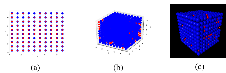
Figure 5: Visualizations of the particle positions, which were assigned initially to a cubic lattice.

For a fancier three-dimensional visualization of the particles, the powerful package VPython is useful.

from vpython import *
for i in range(N):
  tx=x[i]
  ty=y[i]
  tz=z[i]
  if i < Na :
    sphere(pos=vector(tx,ty,tz),radius=0.5,color=color.blue)
  else:
    sphere(pos=vector(tx,ty,tz),radius=0.2,color=color.red)

Use the right mouse button to rotate the plot and the middle mouse button to zoom in and out [see Fig. 5(c)]. More information on plotting tools is available at Ref. newmanOnline, and their external links. The Python program and the initial configuration file for this section are in the files KALJ_initpos.py and initpos available at Ref. supplement, .

III.3 Initialization of velocities

If the positions and velocities are already available, they can be read from a file with six columns, similar to our earlier example. As described in Sec. II.5.1 a temperature bath can be achieved by periodically resetting all velocities from the Maxwell-Boltzmann distribution at the desired temperature. We therefore define a function for this task.

def maxwellboltzmannvel(temp):
  global vx
  global vy
  global vz
  nopart=len(vx)
  sigma=np.sqrt(temp) #sqrt(kT/m)
  vx=np.random.normal(0.0,sigma,nopart)
  vy=np.random.normal(0.0,sigma,nopart)
  vz=np.random.normal(0.0,sigma,nopart)
#  make sure that center of mass does not drift
  vx -= sum(vx)/float(nopart)
  vy -= sum(vy)/float(nopart)
  vz -= sum(vz)/float(nopart)
#  make sure that temperature is exactly wanted temperature
  scalefactor = np.sqrt(3.0*temp*nopart/sum(vx*vx+vy*vy+vz*vz))
  vx *= scalefactor
  vy *= scalefactor
  vz *= scalefactor

This function is used in the example using the Python command maxwellboltzmannvel(0.2) with $T=0.2$. To check the resulting velocities we save them in a file, plot them, and/or visualize them in VPython with

arrow(pos=vector(tx,ty,tz), axis=vector(tvx,tvy,tvz),color=color.green)

where tx,ty,tz correspond to the positions and tvx,tvy,tvz correspond to the velocities. The implementation for this section is in KALJ_initposvel.py.supplement

III.4 Accelerations

As shown in Fig. 3, the accelerations $\mathbf{a}_{i}$ are determined after the initialization and at each time step. A user-defined function for determining the accelerations is therefore recommended.(see Problem 5). For the KA-LJ system, $m_{i}=1$ and $F_{i,x}$ as given in Eq. (6) (similarly $F_{i,y}$ and $F_{i,z}$). We store the accelerations in arrays ax, ay, az. To determine $\mathbf{a}_{i}$ for all $i=1,\ldots,N$ (in Python particle index i=0,$\ldots$,N-1), we need a loop over $i$ and implement the sum over neighbors using an inner loop over $j$. From Newton’s third law, $\mathbf{F}_{ij}=-\mathbf{F}_{ji}$, we can reduce this double sum by a half.

def acceleration(x,y,z):
  ax=sp.zeros(N)
  ay=sp.zeros(N)
  az=sp.zeros(N)
  for i in range(N-1):
    ...
    for j in range(i+1,N):
      ...
      ax[i] += ...
      ax[j] -= ...
      ...

To determine $r_{ij}^{2}$ we use rijto2,

def acceleration(x,y,z):
  ax=sp.zeros(N)
  ...
  for i in range(N-1):
    xi=x[i]
    yi=y[i]
    zi=z[i]
    for j in range(i+1,N):
      xij=xi-x[j]
      yij=yi-y[j]
      zij=zi-z[j]
      ...
      rijto2 = xij*xij + yij*yij + zij*zij
      ...

In addition, we need to implement the minimum image convention as described in Sec. II.3.

def acceleration(x,y,z):
  global L
  global Ldiv2
   ...
      xij=xi-x[j]
      yij=yi-y[j]
      zij=zi-z[j]
      # minimum image convention
      if xij > Ldiv2: xij -= L
      elif xij < - Ldiv2: xij  += L
      if yij > Ldiv2: yij -= L
      elif yij < - Ldiv2: yij  += L
      if zij > Ldiv2: zij -= L
      elif zij < - Ldiv2: zij  += L
      rijto2 = xij*xij + yij*yij + zij*zij
      ...

Here Ldiv2 is $L/2.0$, and we assume the particle positions satisfy $0<x,y,z<L$, which means that x, y, z are updated with periodic boundary conditions to stay within the central simulation box. Because the sum is only over neighbors within $2.5\sigma$ of a given particle, we add an if statement:

def acceleration(x,y,z):
  ...
     rijto2 = xij*xij + yij*yij + zij*zij
     if(rijto2 < rcutto2):
       onedivrijto2 = 1.0/rijto2
       fmagtmp= eps*(sigmato12*onedivrijto2**7 - 0.5*sigmato6*onedivrijto2**4)
       ax[i] += fmagtmp*xij
       ax[j] -= fmagtmp*xij
       ...
  return 48*ax,48*ay,48*az

We avoided the additional costly computational determination of $r_{ij}=\sqrt{r_{ij}^{2}}$, and the factor 48 was multiplied only once via matrix multiplication. This acceleration function is called in the main program with the statement

ax,ay,az = acceleration(x,y,z)

The variables $\mbox{\tt rcutto2}=(r^{\rm cut})^{2}$, $\mbox{\tt eps}=\epsilon$, $\mbox{\tt sigmato12}=\sigma^{12}$, and $\mbox{\tt sigmato6}=\sigma^{6}$ are particle type dependent for the binary Kob-Andersen model. We include this dependence with conditional statements

...
  for i in range(N-1):
    ...
    for j in range(i+1,N):
      ...
      if i < Na:
        if j < Na:   #AA
           rcutto2 = rcutAAto2
           sigmato12 = sigmaAAto12
           sigmato6 = sigmaAAto6
           eps = epsAA
        else:            #AB
           rcutto2 = rcutABto2
           sigmato12 = sigmaABto12
           sigmato6 = sigmaABto6
           eps = epsAB
      else:              #BB

These conditional statements cost computer time and can be avoided by replacing the i, j loops with three separate i, j loops.

# AA interactions
  for i in range(Na-1):
    ...
    for j in range(i+1,Na):
      ...
      rijto2 = xij*xij + yij*yij + zij*zij
      if(rijto2 < rcutAAto2):
        onedivrijto2 = 1.0/rijto2
        fmagtmp= epsAA*(sigmaAAto12*onedivrijto2**7 - 0.5*sigmaAAto6*onedivrijto2**4)
        ...
# AB interactions
  for i in range(Na):
    ...
    for j in range(Na,N):
      ...
      rijto2 = xij*xij + yij*yij + zij*zij
      if(rijto2 < rcutABto2):
        onedivrijto2 = 1.0/rijto2
        fmagtmp= epsAB*(sigmaABto12*onedivrijto2**7 - 0.5*sigmaABto6*onedivrijto2**4)
        ...
# BB interactions
  for i in range(Na,N-1):
    ...
    for j in range(i+1,N):
      ...
  return 48*ax,48*ay,48*az

III.5 NVE molecular dynamics simulation

We are now equipped to implement a NVE molecular dynamics simulation (see Problem 6). We follow the flow chart of Fig. 3 and after the initialization of $\left\{\mathbf{r}_{i}\right\}$, $\left\{\mathbf{v}_{i}\right\}$, and $\left\{\mathbf{a}_{i}\right\}$, add a loop over time steps and update the positions and velocities within this loop. To update $\mathbf{r}_{i}$ and $\mathbf{v}_{i}$ for all $i$, we use matrix operations instead of for loops, because matrix operations are computationally faster in Python. We need to ensure periodic boundary conditions, which we implement assuming that we start with $0<x_{i},y_{i},z_{i}\leq L$ and that during each time step no particle moves further than $L$.

for tstep in range(1,nMD+1):
  # update positions
  x += vx*Deltat + 0.5*ax*Deltatto2
  y += vy*Deltat + 0.5*ay*Deltatto2
  z += vz*Deltat + 0.5*az*Deltatto2
  # periodic boundary conditions:
  for i in range(N):
    if x[i] > L: x[i] -= L
    elif x[i] <= 0:  x[i] += L
    if y[i] > L: y[i] -= L
    elif y[i] <= 0:  y[i] += L
    if z[i] > L: z[i] -= L
    elif z[i] <= 0:  z[i] += L
  # update velocities
  vx += 0.5*ax*Deltat
  vy += 0.5*ay*Deltat
  vz += 0.5*az*Deltat
  ax,ay,az = acceleration(x,y,z)
  vx += 0.5*ax*Deltat
  vy += 0.5*ay*Deltat
  vz += 0.5*az*Deltat

Here ${\tt{nMD}}=n_{\rm MD}$ is the number of time steps, ${\tt Deltat}=\Delta t$, and ${\tt Deltatto2}=(\Delta t)^{2}$.

The most time consuming part of the time loop is the determination of $\left\{\mathbf{a}_{i}\right\}$, because it includes the double loop over $i$ and $j$. In more optimized MD programs, the loop over $j$ would be significantly sped up by looping only over neighbors of particle $i$ (instead of over all particles $j$) via a neighbor list.allen90 However, for our purpose of becoming familiar with MD, we will do without a neighbor list.

III.6 Python: More analysis and visualization tools

As a check of the program, we may either plot the trajectories of a specified particle (see Fig. 6) or make a scatter plot of the initial and final configuration as shown in Fig. 7 for $z(x)$ after $n_{\rm MD}=50$ time steps with $\Delta t=0.005$.

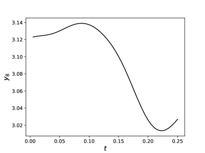
Figure 6: The $y$-component of particle 8 as a function of time $t$ (in LJ time units $\sqrt{m_{A}\sigma_{AA}^{2}/\epsilon_{AA}}$) for the Kob-Andersen model of $N=1000$ particles starting with the initial configuration initposvel, and for $50$ time steps with $\Delta t=0.005$. (The largest time is $50\times 0.005=0.25$.)

For Fig. 6 we used the plot tools as described in Sec. III.2. To plot the $y$-component of particle 8, an array for these values was defined before the time loop

yiplotarray = np.zeros(nMD,float)

This array was updated within the time loop after the time step

yiplotarray[tstep-1]=y[7]

Note that particle 8 corresponds to index 7. After the time loop the following plotting commands are used:

tarray = np.arange(Deltat,(nMD+1)*Deltat,Deltat)
plt.rcParams[’xtick.labelsize’]=11
plt.rcParams[’ytick.labelsize’]=11
plt.figure()
plt.plot(tarray,yiplotarray,color=’blue’)
plt.xlabel(’$t$’,fontsize=15)
plt.ylabel(’$y_8$’,fontsize=15)
plt.show()

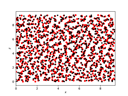
Figure 7: $z(x)$ for the initial configuration in black small circles and for the final configuration at $t=0.25$ (in LJ time units $\sqrt{m_{A}\sigma_{AA}^{2}/\epsilon_{AA}}$) in red large circles.

To make Fig. 7 we stored the initial configuration using

x0 = np.copy(x)
y0 = np.copy(y)
z0 = np.copy(z)

and used plt.scatter as described in Sec. III.2.

We can also make an animation using VPython.newmanOnline Before the time loop we create spheres (particles at their positions) and arrows (velocities) as

s = np.empty(N,sphere)
ar = np.empty(N,arrow)
for i in range(N):
  if i < Na :
    s[i] = sphere(pos=vector(x[i],y[i],z[i]),radius=0.5,color=color.blue)
  else:
    s[i] = sphere(pos=vector(x[i],y[i],z[i]),radius=0.2,color=color.red)
  ar[i]=arrow(pos=vector(x[i],y[i],z[i]),axis=vector(vx[i],vy[i],vz[i]),
          color=color.green)

Within the time loop we update the spheres and arrows as

  rate(30)
  for i in range(N):
    s[i].pos = vector(x[i],y[i],z[i])
    ar[i].pos = vector(x[i],y[i],z[i])
    ar[i].axis = vector(vx[i],vy[i],vz[i])

We can also plot the kinetic energy per particle $E_{\rm kin}/N$, potential energy per particle $V/N$, and the total energy per particle $E_{\rm tot}/N=\left(E_{\rm kin}+V\right)/N$ as a function of time. To include the minimum image convention and the cases $AA$, $AB$, and $BB$, a user-defined function can be written similar to acceleration of Sec. III.4. The Python program for this section, KALJ_nve.py, including the accelerations in Sec. III.4, is available in Ref. supplement, .

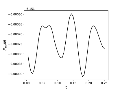
Figure 8: The total energy per particle $E_{\rm tot}/N=\left(E_{\rm kin}+V\right)/N$ as a function of time (in LJ units) for a NVE simulation with $n_{\rm MD}=50$ and with $\Delta t=0.005$. The value $-6.161$ on the top left indicates that the tick labels on the vertical axis are $E_{\rm tot}/N+6.151$. The initial positions and velocities were read in from the file initposvel ($T=0.5$).

As shown in Fig. 8, $E_{\rm tot}/N$ exhibits very small variations about a constant as expected for the NVE simulation.

III.7 NVT molecular dynamics simulation

We now implement a statistical temperature bath as described in Sec. II.5.1, which will allow readers to do simulations at desired temperatures (see Problem 7).

We need to update all the velocities using the Maxwell-Boltzmann distribution specified in Eqs. (11) and (12). Because we already have implemented the Maxwell-Boltzmann distribution in Sec. III.3 with the user-defined function maxwellboltzmannvel, we can implement the temperature bath with only two lines in the time loop after the time step. For the case of computing new velocities every nstepBoltz time steps:

  if (tstep % nstepBoltz) == 0 :
    maxwellboltzmannvel(temperature)

You can test your program by plotting the temperature as a function of time. The temperature can be determined by solving Eq. (13) for $T$. Figure 9 shows an example of a MD simulation using positions initially equilibrated at $T=0.5$, and then run at $T=0.2$. The Python program, KALJ_nvt.py, for this section is available at Ref. supplement, .

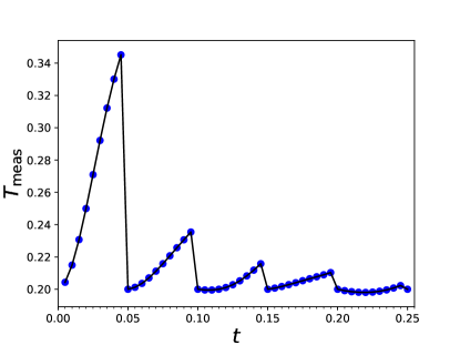
Figure 9: The time-dependence of the temperature for fixed NVT with $T=0.2$, ${\tt nstepBoltz}=10$, and $n_{\rm MD}=50$ with $\Delta t=0.005$.

IV Implementation of MD simulations with LAMMPS

Readers might have noticed that the simulation we have discussed was for only $1000$ particles and $50$ time steps and took painfully long. (The pain level depends on the computer.) To shorten the computation time, there exist optimization techniques such as nearest neighbor lists, as well as coding for multiple processors. We now introduce the free and open source software, LAMMPS. LAMMPS (Large-scale Atomic/Molecular Massively Parallel Simulator) allows a very wide range of simulation techniques and physical systems. The LAMMPS websiteLAMMPSwebpage includes an overview, tutorials, well written manual pages, and links for downloading it for a variety of operating systems. The goal of this section is to help readers get started with LAMMPS and is not a thorough introduction to LAMMPS.

IV.1 Introduction to LAMMPS

In LAMMPS the user chooses the simulation technique, system, particle interactions, and parameters, all via an input file. The main communication between the user and LAMMPS occurs via the input file. To run LAMMPS with parallel code, the simulation is started with commands such as

mpirun -np 16 lmp_mpi < inKALJ_nve > outLJnve

where -np 16 specifies the number of cores, lmp_mpi is the name of the LAMMPS executable (which might have a different name depending on the computer), outLJnve is the output file (see the following for a description on what information is written into this file), and inKALJ_nve is the input file. Becoming familiar with LAMMPS mainly requires learning the commands in this input file. Further documentation can be found at Ref. LAMMPSwebpage, . A set of input file examples is available at Ref. LAMMPSdownload, . Appendix C describes how to run LAMMPS on a shared computer using a batch system.

IV.2 NVE simulation with LAMMPS

To run at fixed NVE the input file, inKALJ_nve, contains

#KALJ NVE, read data
atom_style atomic
boundary p p p #periodic boundary cond. in each direction
read_data initconf_T05eq.data #read data file (incl.mass)
pair_style  lj/cut 2.5  # Define interaction potential
pair_coeff  1 1  1.0 1.0  2.5  #type type eps sigma rcut
pair_coeff  1 2  1.5 0.80 2.0  #typeA typeB epsAB sigmaAB rcutAB=2.5*0.8=2.0
pair_coeff  2 2  0.5 0.88 2.2  #typeB typeB epsBB sigmaBB rcutBB=2.5*0.88=2.2
timestep 0.005 #Delta t
neighbor          0.3 bin
neigh_modify      every 1 delay 0 check yes
dump mydump all custom 50 confdump.*.data id type x y z vx vy vz
dump_modify mydump sort id
# set numerical integrator
fix nve1 all nve # NVE; default is velocity verlet
run 100

Comments start with #. The statement atom_style atomic specifies the type of particle, and boundary p p p implements periodic boundary conditions. Not included in this sample input file are the two possible commands,

units    lj
dimension 3

because they are the default settings.

Initial positions and velocities are read from the file initconf_T05eq.data. For the LAMMPS read_data command, the specified file (here initconf_T05eq.data) contains

#bin. KALJ data file T=0.5

1000 atoms
2 atom types

0 9.4 xlo xhi
0 9.4 ylo yhi
0 9.4 zlo zhi

Masses

1 1.0
2 1.0

Atoms

1 1 2.24399 2.3078 9.07631
2 1 8.54631 2.43192 8.67359
...
1000 2 6.99911 8.89427 6.16712

Velocities

1 0.195617 1.29979 -1.17318
2 -0.905996 0.0649236 0.246998
...
1000 -0.661298 -1.71996 2.00882

The first few lines specify the type of system, $N=1000$ atoms with $A$ and $B$ particles, the box length, $L=9.4$, and the masses $m_{A}=m_{B}=1$. The $1000$ lines following Atoms specify the particle index, $i=1,2,\ldots,1000$ in the first column, the particle type in the second column; that is, 1 for particles $1,2,\ldots,800$ ($A$-particles) and 2 for particles $801,\ldots,1000$ ($B$-particles). Columns three, four, and five are $x_{i}$, $y_{i}$, $z_{i}$ respectively. The lines following Velocities contain $i$, $v_{x,i}$, $v_{y,i}$, and $v_{z,i}$.

In the input file inKALJ_nve the particle interactions are defined by the commands pair_style and pair_coeff. Note that lj/cut corresponds to the forces of Eq. (6). However, the potential energy excludes the term $V_{\alpha\beta}(r^{\rm cut}_{\alpha\beta})$ of Eq. (5). In LAMMPS there is also the option of the truncated and force shifted Lennard-Jones interactions lj/smooth/linear. We chose lj/cut to allow for the direct comparison of the Python and LAMMPS simulations. In the file inKALJ_nve the line timestep 0.005 sets $\Delta t=0.005$. The commands neighbor and neigh_modify are parameters for the neighbor list. The LAMMPS commands dump and dump_modify periodically save snapshots of all atoms. In our example, every 50 time steps (starting with $t=0$) a file is written with file name confdump.0.data, confdump.50.data, confdump.100.data, and the content of each written file has columns $i$, particle type (1 or 2), $x_{i}$, $y_{i}$, $z_{i}$, $v_{x,i}$, $v_{y,i}$, and $v_{z,i}$. In the dump command mydump is the LAMMPS-ID for this dump command. It can be replaced with any name the reader chooses. The ID allows further specifications for this dump as used in the command dump_modify mydump sort id, which ensures that the lines in the dump files are sorted by particle index $i$.

The integration technique is set by the command fix nve1 all nve; nve1 is an ID for this fix command, all means that this integration step is applied to all particles, and nve specifies the NVE time step which is the velocity Verlet integration step by default. The command run100 means that the simulation is run for $100$ time steps under these specified conditions.

The input file inKALJ_nve assumes that the initial positions and velocities are available. For a small system such as $N=1000$ the initial positions may be generated by doing a simulation with Python. However, for simulations with significantly more particles, the initial positions and velocities may not be available. If we instead initialize with uniformly randomly distributed positions and velocities from the Maxwell-Boltzmann distribution, we replace in inKALJ_nve the read_data command with the following LAMMPS commands

region my_region block 0 9.4 0 9.4 0 9.4
create_box 2 my_region
create_atoms 1 random 800 229609 my_region
create_atoms 2 random 200 691203 my_region
mass 1 1
mass 2 1
velocity all create 0.5 92561 dist gaussian

The first two commands create the simulation box for two types of atoms, the create_atoms commands initialize the atom positions randomly drawn from a uniform distribution and random number generator seeds 229609 and 691203 (any positive integers), and the last command initializes the velocities of all particles with the Maxwell-Boltzmann distribution for temperature $T=0.5$ and random number seed 92561.

As noted in Sec. II.6, random positions can lead to very large forces. These can be avoided by adding in inKALJ_nve before the fix command the line

minimize 1.0e-4 1.0e-6 1000 1000

The files (inKALJ_nve, inKALJ_nve_rndposvel, initconf_T05eq.data, and runKALJ_slurm.sh) for this section and the previous two sections are available.supplement

IV.3 NVT simulations

The default NVT simulation in LAMMPS uses the Nosé-Hoover algorithm (see Sec. II.5.2, and Appendices A and B). LAMMPSfixnvtp ; shinoda2004 ; martynaKleinTuckermanJCP1992 ; martynaMolPhys1996 ; martynaJCP1994 ; Frenkel2002 To implement this temperature bath in LAMMPS, we replace the command fix nve1 all nve in the input file with

fix nose all nvt temp 0.2 0.2 $(100.0*dt)

As described in Ref. LAMMPSfixnvtp, , nose is the ID chosen by the user for this fix command, all indicates that this fix is applied to all atoms, nvt temp 0.2 0.2 sets the constant temperature to $T=0.2$, and the last parameter sets the damping parameter as recommended in Ref. LAMMPSfixnvtp, to $100\Delta t$.

Another way of achieving a temperature bath is to implement the statistical temperature bath as described in Sec. II.5.1. We use an implementation similar to that used in Python in Sec. III.7. To compute random velocities periodically in time, we replace the command run 100. To compute new velocities every $10$ time steps at temperature $T=0.2$ the replacement line is

run 100 pre no every 10 "velocity all create 0.2 ${rnd} dist gaussian"

where ${rnd} is a user-defined LAMMPS variable corresponding to a random reproducible integer; rnd needs to be defined before the modified run command by

variable rnd equal floor(random(1,100000,3259))

where we used the LAMMPS function random (see Ref. LAMMPSvariable, ). To test the program, readers may plot the measured temperature as a function of time, $T_{\rm meas}(t)$ (similar to Fig. 9) and $E_{\rm tot}/N$ as a function of time (similar to Fig. 8). Such time dependent functions can be computed and saved with thermo_style,

thermo_style custom step temp pe ke etotal
thermo 2 #print every 2 time steps

which saves data every $2$ time steps in the output file, e.g., outLJnvt, the five variables: (number of time steps), $T_{\rm meas}$, $V/N$, $E_{\rm kin}/N$, and $E_{\rm tot}/N$. Note that the LAMMPS interaction lj/cut potential energy excludes the term $V_{\alpha\beta}(r^{\rm cut}_{\alpha\beta})$ of Eq. (5).

Because the output file includes the output from the thermo command plus several lines with other information, it is convenient to filter out the time dependent information. This can be done in Unix/Linux. For example, to obtain $T_{\rm meas}$ as a function of time steps, use the Unix command

gawk ’NF ==5 && ! /[a-z,A-Z]/ {print $1,$2}’ outLJnvt

The resultant output can be redirected into a file or directly piped into a plotting tool, e.g., by adding to gawk at the end | xmgrace -pipe. To obtain $E_{\rm tot}/N$ as a function of the number of time steps, we replace the gawk command $2 by $5.

The LAMMPS input files, inKALJ_nvt_stat and inKALJ_nvt_Nose, are available at Ref. supplement, .

V Simulation Run Sequence

Readers can now run molecular dynamics simulations with Python or LAMMPS. To illustrate what a simulation sequence entails, we give a few examples of simulations for the Kob-Andersen model.

The first set of papers on the Kob-Andersen model were on the equilibrium properties of supercooled liquids.kobAndersenPRL1994 ; kobAndersenPRE51_1995 ; kobAndersenPRE52_1995 As described in Ref. kobAndersenPRE51_1995, , the system was first equilibrated at $T=5.0$ and then simulated at successively lower temperatures $T=4.0$, $3.0$, $2.0$, $\ldots$, $0.475$, $0.466$. For each successive temperature, a configuration was taken from the previously equilibrated temperature run, the temperature bath (stochastic in this study) was applied for $t_{\rm equi}$ time units, followed by an NVE simulation run also for $t_{\rm equi}$ time units, and then followed by an NVE production run during which the dynamics and structure of the system were determined. This sequence of reaching successively lower temperatures was applied to eight independent initial configurations.

Another example for a simulation sequence is to apply a constant cooling rate as was done in Ref. KVLKobBinder_1996, with an NPT algorithm.

References kobBarratPRL1997, ; kobBarratPhysicaA1999, ; kobetalJPhysCondMat2000, studied the Kob-Andersen model out of equilibrium by first equilibrating the system at a high temperature $T_{\rm i}$ and then quenching instantly to a lower temperature $T_{\rm f}$. That is, a well equilibrated configuration from the simulation at $T_{\rm i}$ was taken to be the initial configuration for an NVT simulation at $T_{\rm f}$. During the run at $T_{\rm f}$ the structure and dynamics of the system depend on the waiting time, which is the time elapsed since the temperature quench. kobBarratPRL1997 ; kobBarratPhysicaA1999 ; kobetalJPhysCondMat2000

VI Analysis

In this section we discuss the analysis of molecular dynamics simulations. To give readers a taste of the wide variety of analysis tools, we focus on two commonly studied quantities: the radial distribution function and the mean square displacement.

VI.1 Radial distribution function

The radial distribution function, $g(r)$, is an example of a structural quantity and is a measure of the density of particles $j$ at a distance $r$ from a particle $i$, where $r=r_{ij}=\left|{\mathbf{r}}_{i}-{\mathbf{r}}_{j}\right|$ and radial symmetry is assumed. For a binary system $g_{AA}(r)$, $g_{BB}(r)$, and $g_{AB}(r)$ are defined as

$$g_{\alpha\alpha}(r)=\frac{V}{N_{\alpha}\left(N_{\alpha}-1\right)}\left\langle\sum\limits_{i=1}^{N_{\alpha}}\sum_{\begin{subarray}{c}j=1\\ j\neq i\end{subarray}}^{N_{\alpha}}\delta\left(r-\left|{\mathbf{r}}_{i}-{\mathbf{r}}_{j}\right|\right)\right\rangle,$$ (18)

where $\alpha\in\{A,B\}$, and (see Refs. kobAndersenPRE51_1995, ; allen90, )

$$g_{AB}(r)=\frac{V}{N_{A}N_{B}}\left\langle\sum\limits_{i=1}^{N_{A}}\sum\limits_{j=1}^{N_{B}}\delta\left(r-\left|{\mathbf{r}}_{i}-{\mathbf{r}}_{j}\right|\right)\right\rangle.$$ (19)

Equations (18) and (19) include sums over particle pairs $(i,j)$ of the types specified. The Dirac delta function $\delta(x)$ is the number density for a point particle at $x=0$. The number density of $(i,j)$ pairs with distance $r=r_{ij}$ is normalized by the global density. Therefore $g(r)$ characterizes the distribution of particle distances. The average $\langle\ldots\rangle$ in Eqs. (18) and (19) can be taken either by averaging over independent simulation runs and/or via a time average by averaging measurements at different times $t$. For the measurement of $g(r)$ in equilibrium, the system needs to be first equilibrated, and therefore $t>t_{\rm equil}$ for all measurements. For more advanced readers the generalization of the radial distribution function is the van Hove correlation function $G(r,t)$.HansenVerlet1969 ; kobAndersenPRE51_1995

VI.1.1 Radial distribution function with Python

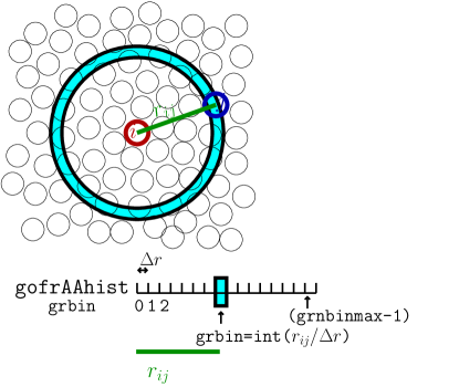
Figure 10: Sketch of the determination of the radial distribution function. To compute $g_{AA}(r)$ a histogram of pair distances $r_{ij}$ is stored in the array gofrAAhist. The width of each bin is $\Delta r$. There are grnbinmax bins.

To determine a histogram of the $r_{ij}$ distances, we use an array as illustrated for $g_{AA}$ in Fig. 10. Before determining the histogram we set to zero the arrays gofrAAhist, gofrBBhist, and gofrABhist. For each measurement, we loop over all unique particle combinations ($j>i$), determine the minimum image distance (see Sec. III.4), and add to the counter of the corresponding bin.allen90

for i in range(0,N-1):
  xi=x[i]
  ...
  for j in range(i+1,N):
    xij=xi-x[j]
    ...
    #minimum image convention
    if xij > Ldiv2: xij -= L
    ...
    rijto2 = xij*xij + yij*yij + zij*zij
    rij=sp.sqrt(rijto2)
    grbin=int(rij/grdelta)
    if(grbin < grnbinmax):
      if(i < Na):
        if (j < Na): #AA
          histgofrAA[grbin] += 2
        else: #AB
          histgofrAB[grbin] += 1
      else: #BB
        histgofrBB[grbin] += 2

Here ${\tt grdelta}=\Delta r$ is the bin size (see Fig. 10). If the average is a time average, taken via measurements (assume with user defined function histmeas) after tequil time steps every nstepgofr time steps, we set the arrays histgofrAA etc. to zero before the time loop, and add the conditional statement

if (tstep > tequil) and ((tstep % nstepgofr)==0):
   histmeas(x,y,z)

within the time loop and after the time step, that is in the flow chart of Fig. 3 after the (blue) “Time Step” box and within the “Loop Over Time Steps,” so before the (green) time loop repeats. We can then save the resulting radial distribution functions into a file of name gofrAABBAB.data by adding to the program after the time loop

fileoutgofr= open("gofrAABBAB.data",mode=’w’)
for grbin in range(grnbinmax):
  rinner = grbin*grdelta
  router = rinner + grdelta
  shellvol = (4.0*sp.pi/3.0)*(router**3 - rinner**3)
  gofrAA = (L**3/(Na*(Na-1)))*histgofrAA[grbin]/(shellvol*nmeas)
  gofrBB = (L**3/(Nb*(Nb-1)))*histgofrBB[grbin]/(shellvol*nmeas)
  gofrAB = (L**3/(Na*Nb))*histgofrAB[grbin]/(shellvol*nmeas)
  rmid = rinner + 0.5*grdelta
  print(rmid,gofrAA,gofrBB,gofrAB,file=fileoutgofr)

We have assumed that nmeas measurements of the histogram were taken, and the variables are as shown in Fig. 10 with ${\tt grdelta}=\Delta r$. For the normalization we determine the shell volume/area, which is sketched in Fig. 10 as the cyan (gray) shaded area enclosed by the two large circles drawn with thick lines. In three dimensions the shell volume is $(4\pi/3)\left(r_{\rm outer}^{3}-r_{\rm inner}^{3}\right)$.

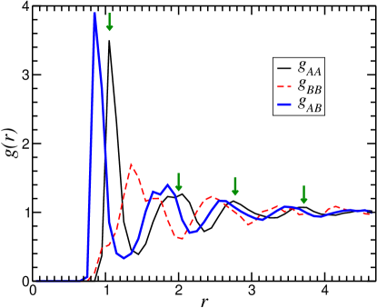
Figure 11: Radial pair distribution functions for the Kob-Andersen model with $N=1000$, $L=9.4$ at $T=0.5$. The green vertical arrows indicate peak positions of $g_{AA}(r)$.

The resulting radial distribution functions are shown in Fig. 11 for which we ran the NVT simulation with $N=1000$ at $T=0.5$, starting with a well equilibrated configuration at $T=0.5$, running the simulation for $200$ time steps and measuring the histogram every nstepgofr=25 time steps with $\Delta r=0.1$. To measure distances up to $L/2$, we set grnbinmax = int(Ldiv2/grdelta). The Python program KALJ_nvt_gofr.py for this section is in Ref. supplement, .

VI.1.2 Interpretation of radial distribution function

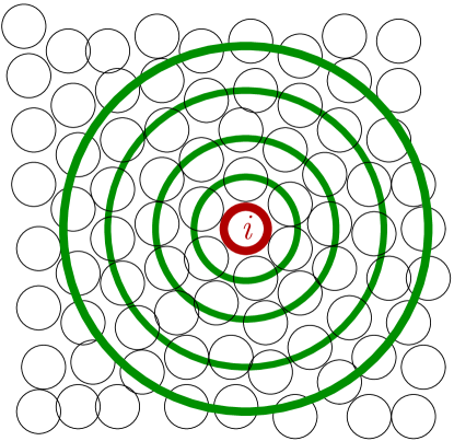
Figure 12: Sketch of particle arrangements to illustrate the interpretation of the radial distribution function. The first, second, third, and forth neighbor shells are indicated with dark green circles (thick lines). The radii of these shells correspond to the peak positions of the radial distribution function as indicated with dark green vertical arrows in Fig. 11 for the example of $g_{AA}(r)$.

Because the repulsive interaction $V(r_{ij}\to 0)\to\infty$ prevents the complete overlap of two particles, $g(r)=0$. The first peak of $g(r)$ corresponds to the most likely radius of the first shell of neighboring particles surrounding particle $i$. The second peak of $g(r)$ corresponds to the second nearest neighbor shell, etc. (see Fig. 12). With increasing $r$ the peaks become less and less pronounced, because the system has, contrary to a crystal, no long range order. The peak positions of $g_{AA}(r)$, $g_{BB}(r)$, and $g_{AB}(r)$ in Fig. 11 are consistent with the results of Kob and Andersen (Fig. 9 of Ref. kobAndersenPRE51_1995, ). For their more quantitative study, they used longer simulation runs, several independent simulation runs, and a smaller (and probably more than one) value of $\Delta r$.

VI.1.3 Radial distribution function with LAMMPS

We can determine the radial distribution functions with LAMMPS by adding to the input file before the run command the lines

compute rdfAABBAB all rdf 25 1 1 2 2 1 2
fix myrdf all ave/time 25 8 200 c_rdfAABBAB[*] file gofrAABBAB.data mode vector

The compute command defines the measurements, which are done during the run:

1. rdfAABBAB is the user defined ID for this compute command. This ID is used in the fix command with c_rdfAABBAB, which means the ID is like a variable name.

2. all applies the command to all atoms.

3. rdf computes the radial distribution function.

4. ${\tt 25}=N_{\rm bin}$ specifies $\Delta r$ to be $r^{\rm cut}/25$. The following numbers specify the particle type combinations, that is, $g_{AA}$, $g_{BB}$, and $g_{AB}$.

5. fix ave/time defines the time averaging. As described in Ref. LAMMPSfixavetime, the three numbers in our example specify that the histogram is measured every $\mbox{\tt Nevery}=25$ time steps, ${\tt Nrepeat}=8$ measurements are averaged (in Sec. VI.1.1 nmeas), and ${\tt Nfreq}=200$ is the interval of time steps at which the time average is printed. That is, if the simulation run is $n_{\rm MD}=600$, then the averages of $g(r)$ are printed out three times, the first by averaging measurements taken at time step $200,175,150,\ldots,25$, and the last one at time steps $600,575,550,\ldots,425$. Constraints on the choice of Nevery, Nrepeat, and Nfreq are given in Ref. LAMMPSfixavetime, . In addition, compatible times need to be chosen, if the LAMMPS command run every is used, which we used for the statistical temperature bath in Sec. IV.3.

6. [*] takes time averages for each of the variables of the compute rdf command

7. file gofrAABBAB.data specifies that the results are saved in the file gofrAABBAB.data.

8. mode vector is necessary, because $g_{AA}(r)$ etc. are vectors instead of scalars, with indices for the $N_{\rm bin}$ bins $r=[0,\Delta r),[\Delta r,2\Delta r),\ldots$. The entries in the file gofrAABBAB.data are for each average time (here $200$, $400$, $600$) starting with one line specifying the print time in time steps, $200$ etc., and Nevery, followed by $N_{\rm bin}$ lines, each with columns for the bin number, $r$, $g_{AA}$, $c_{AA}$, $g_{BB}$, $c_{BB}$, $g_{AB}$, $c_{AB}$, where $c_{AA}$ etc. are coordination numbers.

The LAMMPS input file inKALJ_T05_gofr is in Ref. supplement, .

VI.2 Mean square displacement

We next study how the system evolves as a function of time. The mean square displacementallen90 ; kobAndersenPRE51_1995 captures how far each particle moves during a time interval $t$:

$$\mbox{msd}=\left\langle r^{2}(t)\right\rangle=\left\langle\left|\mathbf{r}(t)-\mathbf{r}(0)\right|^{2}\right\rangle$$ (20)

where $\langle\ldots\rangle$ corresponds to an average over particles and may also include an average over independent simulation runs. In the following discussion on the implementation of the mean square displacement with Python and mean square displacement with LAMMPS, we average only over particles of one type

$$\left\langle r^{2}_{\alpha}(t)\right\rangle=\frac{1}{N_{\alpha}}\sum\limits_{i=1}^{N_{\alpha}}\left|\mathbf{r}_{i}(t)-\mathbf{r}_{i}(0)\right|^{2},$$ (21)

where $\alpha\in\{A,B\}$ is the particle type.

A generalization of Eq. (20) is

$$\left\langle r^{2}(t_{\rm w},t_{\rm w}+t)\right\rangle=\left\langle\left|\mathbf{r}(t_{\rm w}+t)-\mathbf{r}(t_{\rm w})\right|^{2}\right\rangle$$ (22)

If the system is in equilibrium, $\left\langle r^{2}(t_{\rm w},t_{\rm w}+t)\right\rangle$ is independent of starting time $t_{\rm w}$ and the average $\langle\ldots\rangle$ may include an average over $t_{\rm w}$.

VI.2.1 Mean square displacement with Python

It is suggested that readers do Problem 8 before reading the following. We use arrays to store the positions at $t=0$ after the initialization of the positions with ${\tt x0=np.copy(x)}$, …. We cannot use periodic boundary conditions to determine the mean square displacement and instead use unwrapped coordinates and define the additional arrays xu, yu, and zu which are initially also copied from x, etc. These arrays are updated in the time step loop as in Sec. III.5

  xu += vx*Deltat + 0.5*ax*Deltatto2
  yu += vy*Deltat + 0.5*ay*Deltatto2
  zu += vz*Deltat + 0.5*az*Deltatto2

Periodic boundary conditions are not applied to xu, yu, and zu.

To save the results into the file msd.data, we add before the time loop the statement fileoutmsd = open("msd.data",mode=’w’). Measurements of the mean square displacements are done within the time loop and after the time step.

  msdA = 0.0
  for i in range(Na):
    dx = xu[i]-x0[i]
    dy = yu[i]-y0[i]
    dz = zu[i]-z0[i]
    msdA += dx*dx+dy*dy+dz*dz
  msdA /= float(Na)
  msdB = 0.0
  for i in range(Na,N):
    dx = xu[i]-x0[i]
    dy = yu[i]-y0[i]
    dz = zu[i]-z0[i]
    msdB += dx*dx+dy*dy+dz*dz
  msdB /= float(Nb)
  print(tstep*Deltat,msdA,msdB,file=fileoutmsd)

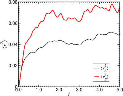
Figure 13: The mean square displacement $\langle r^{2}\rangle$ as function of time $t$ (in LJ units) for the Kob-Andersen model. The initial configuration is equilibrated at $T=0.5$. The results are for a NVE simulation for $N=1000$ and for $1000$ time steps (with a Python program, recording $\langle r^{2}\rangle$ every time step. After a steep increase for very small times, $\langle r^{2}\rangle$ reaches a plateau. For the interpretation of this figure see Sec. VI.2.3.

Figure 13 shows the resultant mean square displacement as a function of time. After a steep increase for very small times, $\langle r^{2}\rangle$ reaches a plateau. The plateau value is larger for the smaller $B$ particles. For significantly longer times $\langle r^{2}\rangle$ increases again. To quantify $\langle r^{2}(t)\rangle$ we need to record every time step for short times and longer and longer time intervals for larger times so that the data points on the horizontal axis are evenly spaced on a log-log plot of $\langle r^{2}(t)\rangle$ as shown in Fig. 14 for a simulation using LAMMPS, which is needed for such larger times. This is achieved by saving data at times $t_{k}=t_{0}*A^{k}$. In terms of time steps

$$\frac{t_{k}}{\Delta t}=\frac{t_{0}}{\Delta t}*A^{k}.$$ (23)

For $k_{\max}$ print times, we solve Eq. (23) for $A$ for the case of $k=k_{\max}$, when $\left(t_{k_{\rm max}}/\Delta t\right)=n_{\rm MD}$ is the total number of time steps.

$$A=\left(\frac{n_{\rm MD}}{\left(t_{0}/\Delta t\right)}\right)^{(1/k_{\max})}$$ (24)

The parameters needed for the calculation of $\langle r^{2}(t)\rangle$ can be set in Python for the example of $n_{\rm MD}=1000$, $\left(t_{0}/\Delta t\right)=1.0$, and $k_{\max}=60$ with the following lines before the time step loop:

kmsdmax = 60
t0msd = 1.0
A=(float(nMD)/t0msd)**(1.0/float(kmsdmax))
tmsd = t0msd
tmsdnextint = int(round(t0msd))

where t0msd$=\left(t_{0}/\Delta t\right)$, and tmsd$=\left(t_{k}/\Delta t\right)$. Within the time step loop we add the conditional statements

  if tmsdnextint == tstep:
    # prepare when next msd-time
    while(tmsdnextint == tstep):
      tmsd = A*tmsd
      tmsdnextint = int(round(tmsd))
    # do measurement
    msdA = 0.0
    for i in range(Na):
      dx = xu[i]-x0[i]
    ...

where ... continues as above for the msd linear in time. The while loop was added, because for short times A*tmsd might increase by less than the integer 1.

The Python programs, KALJ_nve_msd_lin.py and KALJ_nve_msd_log.py, for this section are available in Ref. supplement, .

VI.2.2 Mean square displacement with LAMMPS

The determination of the mean square displacement requires a computation during the simulation run. This computation can be done in LAMMPS with the compute command. (Another example of the compute command is in Sec. VI.1.3 for the computation of $g(r)$.) In Eq. (21) the sum is over only $A$ or $B$ particles. Thus, in the LAMMPS input script we need to define these groups of atoms, which we then use for the following compute commands:

group A type 1
group B type 2
compute msdA A msd
compute msdB B msd

If we wish to save the mean square displacement every time step, or more generally with linear time averaging, we can use the fix ave/time command as described in Sec VI.1.3. To write $\langle r_{A}^{2}\rangle$ and $\langle r_{B}^{2}\rangle$ for every time step into files msdA.data and msdB.data, respectively, we use the commands

fix msdAfix A ave/time 1 1 1 c_msdA[4] file msdA.data
fix msdBfix B ave/time 1 1 1 c_msdB[4] file msdB.data

The resulting files can be used to make a figure. However, as will become clear in Sec. VI.2.3, if long simulation runs of the order of $10^{7}$ time steps are desired, saving in logarithmic time becomes necessary (see Sec. VI.2.1). Logarithmic printing can be achieved by using the functionLAMMPSvariable ; logfreq3 logfreq3 to define the print times tmsd with the variable command and then by using thermo_style and thermo (see Sec. IV.3) to print the mean square displacements into the output file together with other scalar quantities which depend on time. The previous fix ave/time commands are replaced by

variable tmsd equal logfreq3(1,200,10000000)
variable tLJ equal step*dt
thermo_style custom v_tLJ c_msdA[4] c_msdB[4] pe etotal
thermo v_tmsd

We also defined the variable tLJ for the printing of $t$ in LJ units (instead of time steps).logpython

Another way to obtain information logarithmic in time is to print all unwrapped particle positions during the LAMMPS simulation,

variable tmsd equal logfreq3(1,200,10000000)
dump msddump all custom 5000 posudump.*.data id xu yu zu
dump_modify msddump sort id every v_tmsd

and then analyze the resulting posudump* files with Python or another programming language. The LAMMPS input files, inKALJ_nve_msd_lin, inKALJ_nve_msd_log, and inKALJ_nve_msd_logdumps, for this section are in Ref. supplement, .

VI.2.3 Interpretation of mean square displacement

Figure 14 shows $\langle r_{A}^{2}\rangle$ and $\langle r_{B}^{2}\rangle$ obtained with thermo_style as described in Sec. VI.2.2.

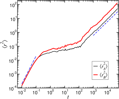
Figure 14: The mean square displacement $\langle r^{2}\rangle$ as a function of the time $t$ (in LJ units) for the Kob-Andersen model. The initial configuration is equilibrated at $T=0.5$. The results are for the NVE simulation with $N=1000$ and for $10^{7}$ time steps (with LAMMPS and saving $\langle r^{2}\rangle$ in logarithmic intervals.)

For very short times $t$, we can approximate $\mathbf{r}_{i}(t)=\mathbf{r}_{i}(0)+\mathbf{v}_{i}(0)\,t$ and write Eq. (21) for small $t$ as

$$\langle r_{\alpha}^{2}\rangle=\frac{1}{N_{\alpha}}\sum\limits_{i=1}^{N_{\alpha}}\left|\mathbf{v}_{i}(0)\,t\right|^{2}=C\,t^{2}.$$ (25)

We see that $\ln\left(\langle r_{\alpha}^{2}\rangle\right)=\ln C+2\ln t$, corresponding to a line with slope $2$ as indicated by the dashed line at short times in Fig. 14.

For intermediate times $\langle r_{\alpha}^{2}\rangle$ reaches a plateau. This plateau is typical for glass formers at high enough density at which each particle is trapped in a cage formed by its neighboring particles. The smaller $B$ particles reach a higher plateau. For long enough times each particle escapes its cage of neighbors and therefore $\langle r_{\alpha}^{2}\rangle$ increases. At very large times the dynamics of many successive escape events can be modeled as a random walk. For a random walk in $d$ dimensions of step size $a$ and an equal probability to step right or left, we have after $N_{\rm step}$ stepsgouldTobochnikChristian2007

$$\langle\left(\Delta\mathbf{r}\right)^{2}\rangle=da^{2}N_{\rm step}.$$ (26)

Equation (26) implies that $\langle r_{\alpha}^{2}\rangle\propto t$ and therefore a log-log plot yields a line of slope $1$ as indicated by a blue dashed line at long times in Fig. 14.

VII Suggested problems

1. Determine $F_{i,x}=-{\rm d}V/{\rm d}x_{i}$.

2. Sketch the flow chart for the molecular dynamics simulation in Fig. 1 in more detail, specifying the order of the determination of positions, velocities, accelerations, and the application of periodic boundary conditions.

3. To derive Eq. (13), first determine $\langle\frac{1}{2}m_{i}v_{i,x}^{2}\rangle=\!\int\limits_{-\infty}^{\infty}\frac{1}{2}m_{i}v_{i,x}^{2}P\left(v_{i,x}\right){\rm d}v_{i,x}$ (the result is a special case of the equipartition theorem), and then obtain Eq. (13).

4. Write a program that places the $N$ particles on lattice sites of a simple cubic lattice.

5. Outline the implementation of the acceleration function and program it with Python.

6. Use Fig. 3 to add to your Python program the loop over time steps and update positions and velocities.

7. Use Sec. II.5.1 to add to your Python program the stochastic temperature bath algorithm.

8. Add to your NVE Python program the determination of the mean square displacement and save the results in a file.

9. For the $(3N+1)$ generalized coordinates $\mathbf{q}=\left(\left\{\mathbf{r}_{i}\right\},s\right)$ determine the conjugate momenta $\mathbf{p}_{i}$ and $p_{s}$ and then the Hamiltonian.

10. To simulate a system of sheared bubbles, DuriandurianPRL1995 ; durianPRE1997 introduced a model such that bubble $i$ of radius $R_{i}$ interacts with bubbles $j$ of radius $R_{j}$ as

    $$V_{ij}=\frac{F_{0}}{2}\left[1-\frac{r_{ij}}{\left(R_{i}+R_{j}\right)}\right]^{2}$$ (27)

    for all $j$ with $r_{ij}\leq\left(R_{i}+R_{j}\right)$. Determine the force $\mathbf{F}_{ij}$ on particle $i$ due to particle $j$. The solution is Eq. (1) in Ref. durianPRE1997, .

11. Compute the radial distribution functions $g_{\alpha\beta}$ for (a) temperatures $0.1\leq T\leq 3.0$ and (b) densities $0.1\leq N/L^{3}\leq 2.0$. For each parameter set, first equilibrate before measuring $g_{\alpha\beta}$. Choose $\Delta r\leq 0.05$. In Python you can include a parameter in the name of the output file. For example, to use the temperature in the name we can write fileoutgofr= open("gofrAABBAB"+str(temperature)+".data",mode=’w’). Interpret your results. Reference kobAndersenPRE51_1995, includes $g_{\alpha\beta}$ for $0.466\leq T\leq 5.0$ in Fig. 9 as well as a discussion of its behavior.

12. Compute the mean square displacement given in Eq. (22). Average over each type of particle separately, that is, compute

    $$\left\langle r^{2}_{\alpha}(t_{\rm w},t_{\rm w}+t)\right\rangle=\frac{1}{N_{\alpha}}\sum\limits_{i=1}^{N_{\alpha}}\left|\mathbf{r}_{i}(t_{\rm w}+t)-\mathbf{r}_{i}(t_{\rm w})\right|^{2}.$$ (28)

    Use several values of $t_{\rm w}$. For example in a run with $n_{\rm MD}=1000$, use $t_{\rm w}=0,10\Delta t,100\Delta t,500\Delta t$. First do a NVE simulation as done in Sec. VI.2. Use as initial configuration the provided file initposvel (for Python) or initconf_T05eq.data (for LAMMPS), which is well equilibrated at $T=0.5$. Make a plot of $\left\langle r^{2}_{\alpha}(t_{\rm w},t_{\rm w}+t)\right\rangle$ as a function of the time difference $t$ for different values of $t_{\rm w}$. Interpret your results. Then, using the same initial configuration file, do a NVT simulation at $T=0.2$. Make again a plot of $\left\langle r^{2}_{\alpha}(t_{\rm w},t_{\rm w}+t)\right\rangle$ as a function of the time difference $t$ for different values of $t_{\rm w}$. Compare your plots for the NVE run ($T=0.5$) and the NVT run at $T=0.2$ and interpret your results.

13. Determine the mean square displacement $\left\langle r^{2}_{\alpha}(t)\right\rangle$ of the KA-LJ system for $N=1000$, $L=9.4$ at temperatures $3.0,2.0,1.0,0.8,0.6,0.55,0.5,$ and $0.475$ (a subset of the temperatures studied by Kob and Andersen.kobAndersenPRE51_1995 Be sure to equilibrate the system sufficiently at each investigated temperature. As in Ref. kobAndersenPRE51_1995, start at $T=3.0$, apply a temperature bath for $n_{{\rm equi},T=3}$ time steps, continue with a NVE simulation run of $n_{{\rm equi},T=3}$ time steps, use the resulting configuration as initial configuration for the production run at $T=3.0$ and also as initial configuration of the next lower temperature, $T=2.0$. Apply the temperature bath at $T=2.0$ for $n_{{\rm equi},T=2}$ time steps, followed by a NVE simulation run of $n_{{\rm equi},T=2}$ time steps, etc. For $\Delta t=0.0025$ we recommend $n_{{\rm equi},T}=10^{6}$ time steps for $T\geq 0.8$, $n_{{\rm equi},T}=2\times 10^{6}$ for $0.6\geq T\geq 0.55$, and $n_{{\rm equi},T}=5\times 10^{6}$ for $0.5\geq T\geq 0.475$. When doing a sequence of NVT and NVE runs, use the LAMMPS command unfix before applying the next fix command. To be able to apply logarithmic printing of the mean square displacement as in Sec. VI.2.2, you may also use the LAMMPS command reset_timestep 0. To ensure that the neighbor list is updated sufficiently frequently, use the LAMMPS command neighbor 0.2 bin (instead of neighbor 0.3 bin). If the Nosé temperature bath is used, we recommend for $T\leq 0.5$ to scale the velocities after the NVT run such that the total energy per particle of the NVE run is equal to the average total energy per particle $\langle E_{\rm tot}/N\rangle$ during the NVT run with the (time) average taken near the end of the NVT run. Velocity scaling can be achieved with the LAMMPS command velocity all scale ${scaleEn}, where {scaleEn} corresponds to the temperature corresponding to the time averaged total energy per particle obtained for example with the LAMMPS commands

    variable etot equal ke+pe
    fix aveEn all ave/time 1 500000 2000000  v_etot
    variable scaleEn equal (2*(f_aveEn-pe))/3
    

    These commands need to be before the run command of the NVT run. Interpret the resulting mean square displacements and compare your results with Fig. 2 of Ref. kobAndersenPRE51_1995, , keeping in mind, that we use the time unit $\sqrt{m_{A}\sigma_{AA}^{2}/\epsilon_{AA}}$, whereas Kob and Andersen use the time unit $\sqrt{m_{A}\sigma_{AA}^{2}/48\epsilon_{AA}}$. For large times $t$ the mean square displacement depends on $t$ as (see Ref. gouldTobochnikChristian2007, )

    $$\left\langle r^{2}_{\alpha}(t)\right\rangle=2dD_{\alpha}t,$$ (29)

    where $D_{\alpha}$ is the diffusion constant for particles $\alpha\in\{A,B\}$. Determine $D_{\alpha}(T)$ by fitting Eq. (29) to $\left\langle r^{2}_{\alpha}(t)\right\rangle$. Fitting can be done for example with Python or gnuplot. For each fit check the goodness of the fit by eye by plotting your data and the fitting curve. To ensure that Eq. (29) is a good approximation adjust the $t$-range used for the fitting accordingly. Use the resulting fit parameters to obtain $D_{A}(T)$ and $D_{B}(T)$. As done in Ref. kobAndersenPRE51_1995, , fit the predictions from mode-coupling theory

    $$D_{\alpha}=A\left(T-T_{\rm c}\right)^{\gamma_{\alpha}},$$ (30)

    and check your fits with a log-log plot of $D_{\alpha}$ as function of $(T-T_{\rm c})$. Another prediction for $D_{\alpha}(T)$ is the Vogel-Fulcher law

    $$D_{\alpha}=C\exp\left[-B/(T-T_{\rm VF}\right]\,.$$ (31)

    Compare your results with Fig. 3 of Ref. kobAndersenPRE51_1995, which shows $6D_{\alpha}$ (not $D_{\alpha}$ DKAFig3 ) with diffusion unit $\sigma_{AA}\sqrt{48\epsilon_{AA}/m_{A}}$ (instead of $\sigma_{AA}\sqrt{\epsilon_{AA}/m_{A}}$ as for your results). The results are discussed in Ref. kobAndersenPRE51_1995, .

14. Simulate the binary Lennard-Jones system in two instead of three dimensions. Choose the same density $N/L^{2}=1.204$ with $N=1000$ and $L=28.82$. Either start with random positions and velocities from a Maxwell-Boltzmann distribution, or use the input file configurations initposvel_2d_lammps.data (for LAMMPS) or initposvel_2d_python.data (for Python). Both are a result of simulations at $T=0.2$ and are provided in Ref. supplement, . Do an NVE or NVT simulation for $T<0.5$. Remember to replace $3$ by $2$ in Eq. (13) and adjust the variable shellvol in the Python computation of the radial distribution function. For LAMMPS follow the instructions in Ref. LAMMPS2d, ; you may set $z_{i}=v_{i,z}=0.0$ with the LAMMPS command set atom 1000 z 0.0 vz 0.0. Make a scatter plot of the resulting particle positions and compute the radial distribution function. Compare with the three-dimensional results. An interpretation of your results is given in Ref. KALJ2dBruening, , which introduced the two-dimensional Kob-Andersen Lennard-Jones model with the particle ratio $N_{A}:N_{B}=65:35$ instead of $80:20$.

Appendix A Hamiltonian Formalism for Nosé-Hoover Thermostat

We motivate Eqs. (14) and (15) using the Hamiltonian formalism. We follow the derivation given in Chapter 6 of Ref. Frenkel2002, and present a shortened version here for simplicity. For a complete derivation see Refs. Frenkel2002, ; nosehoover, ; branka, .

We start with the Lagrangian

$${\cal L} = \sum\limits_{i=1}^{N}\frac{1}{2}m_{i}\left(s\,\dot{\mathbf{r}}_{i}\right)^{2}-V\left(\{\mathbf{r}_{i}\}\right)$$ (32)

$${}+\frac{1}{2}Q\dot{s}^{2}-Xk_{\rm B}T\ln s,$$

where $X=dN$ (see Problem 9). The momenta are $p_{i,x}=\partial{\cal L}/\partial\dot{r}_{i,x}=m_{i}s^{2}\dot{r}_{i,x}$ and similarly for $p_{i,y}$ and $p_{i,z}$. Therefore

$$\mathbf{p}_{i}=m_{i}s^{2}\dot{\mathbf{r}}_{i}$$ (33)

Similarly, $p_{s}=\partial{\cal L}/\partial\dot{s}=Q\dot{s}$. We apply Hamiltonian mechanicsTaylor using as generalized coordinates $q_{k}$ for $k=1,2,\ldots 3N+1$, where the first $3N$ values of $k$ label $q_{k}=r_{i,\mu}$ for particles $i=1,\ldots,N$ and $\mu\in\{x,y,z\}$ and $q_{3N+1}=s$. The corresponding Hamiltonian is

$${\cal H} =\sum\limits_{k=1}^{3N+1}\dot{q}_{k}\,p_{k}-{\cal L}$$ (34)

$$=\sum\limits_{i=1}^{N}\frac{\mathbf{p}_{i}^{2}}{2m_{i}s^{2}}+V\left(\{\mathbf{r}_{i}\}\right)+\frac{p_{s}^{2}}{2Q}+Xk_{\rm B}T\ln s$$ (35)

We use Hamilton’s equations $\dot{q}_{k}=\partial{\cal H}/\partial p_{k}$ and $\dot{p}_{k}=-\partial{\cal H}/\partial q_{k}$ to obtain the equations of motion

$$\dot{\mathbf{r}}_{i} =\frac{\partial{\cal H}}{\partial\mathbf{p}_{i}}=\frac{\mathbf{p}_{i}}{m_{i}s^{2}}$$ (36)

$$\dot{s} =\frac{\partial{\cal H}}{\partial p_{s}}=\frac{p_{s}}{Q}$$ (37)

$$\dot{\mathbf{p}}_{i} =-\frac{\partial{\cal H}}{\partial\mathbf{r}_{i}}=-\nabla_{i}V=\mathbf{F}_{i}$$ (38)

$$\dot{p}_{s} =-\frac{\partial{\cal H}}{\partial s}=\sum\limits_{i=1}^{N}\frac{p_{i}^{2}}{m_{i}s^{3}}-\frac{Xk_{\rm B}T}{s}.$$ (39)

We follow Frenkel and SmitFrenkel2002 and switch to “real variables” $\tilde{\mathbf{r}}_{i}$, $\tilde{\mathbf{p}}_{i}$, $\tilde{s}$, $\tilde{p}_{s}$, ${\rm d}\tilde{t}$, corresponding to a rescaling of the time:

$$\tilde{\mathbf{r}}_{i} =\mathbf{r}_{i}$$ (40)

$$\tilde{\mathbf{p}}_{i} =\frac{\mathbf{p}_{i}}{s}$$ (41)

$$\tilde{s} =s$$ (42)

$$\tilde{p_{s}} =\frac{p_{s}}{s}$$ (43)

$${\rm d}\tilde{t} =\frac{{\rm d}t}{s}$$ (44)

We also define

$$\xi=\frac{{\rm d}s}{{\rm d}t}=\frac{{\rm d}\ln\tilde{s}}{{\rm d}\tilde{t}}$$ (45)

The equations of motion for the real variables are

$$\frac{{\rm d}\tilde{\mathbf{r}}_{i}}{{\rm d}\tilde{t}} =\frac{{\rm d}{\mathbf{r}}_{i}}{\frac{1}{s}{\rm d}{t}}=s\frac{\mathbf{p}_{i}}{m_{i}s^{2}}=\frac{\tilde{\mathbf{p}}_{i}}{m_{i}}$$ (46)

$$\frac{{\rm d}\tilde{\mathbf{p}}_{i}}{{\rm d}\tilde{t}} =s\frac{{\rm d}}{{\rm d}t}\left(\frac{\mathbf{p}_{i}}{s}\right)=\frac{{\rm d}\mathbf{p}_{i}}{{\rm d}t}-\mathbf{p}_{i}\frac{\left(\frac{{\rm d}s}{{\rm d}t}\right)}{s}=\mathbf{F}_{i}-\tilde{\mathbf{p}}_{i}\xi$$ (47)

$$\frac{{\rm d}\xi}{{\rm d}\tilde{t}} =\frac{{\rm d}}{{\rm d}\tilde{t}}\left(\frac{{\rm d}s}{{\rm d}t}\right)=s\frac{\rm d}{{\rm d}t}\left(\frac{p_{s}}{Q}\right)$$

$$=\frac{s}{Q}\left(\sum\limits_{i=1}^{N}\frac{p_{i}^{2}}{m_{i}s^{3}}-\frac{Xk_{\rm B}T}{s}\right)=\frac{1}{Q}\left(\sum\limits_{i=1}^{N}\frac{\tilde{\mathbf{p}}_{i}^{2}}{m_{i}}-Xk_{\rm B}T\right).$$ (48)

By using Eq. (35) the Hamiltonian in terms of real variables can be expressed as

$${\cal H}=\sum\limits_{i=1}^{N}\frac{\tilde{p}_{i}^{2}}{2m_{i}}+V\left(\{\mathbf{r}_{i}\}\right)+\frac{Q}{2}\xi^{2}+Xk_{\rm B}T\ln\tilde{s}.$$ (49)

For the equations of motion (46)–(48) the constant of motion is given by Eq. (49). Note that Eqs. (47) and (48) are the same as Eqs. (14) and (15) by replacing in Eqs. (47) and (48) $\tilde{\mathbf{r}}_{i},\tilde{s},\tilde{\mathbf{p}}_{i},\tilde{p}_{s}$ with $\mathbf{r}_{i},s,\mathbf{p}_{i},p_{s}$; that is, we do a (confusing) change of notation for the sake of simplicity in Sec. II.5.2.

Appendix B Fox-Anderson Integration of the Nosé-Hoover Equations

We cannot directly apply the velocity-Verlet algorithm of Eqs. (7) and (8) to numerically integrate Eqs. (14) and (15) because the acceleration $\mathbf{a}_{i}(t+\Delta t)$ depends on the velocity $\mathbf{v}_{i}(t+\Delta t)$. We use instead the more general velocity Verlet integration technique of Fox and Andersenfox and apply it to the NVT Nosé-Hoover equations of motion. As described in Appendix A of Ref. fox, this technique is applicable when the form of the equations of motion is

$$\ddot{\mathbf{x}}(t) =f[\mathbf{x}(t),\dot{\mathbf{x}}(t),\mathbf{y}(t),\dot{\mathbf{y}}(t)]$$ (50)

$$\ddot{\mathbf{y}}(t) =g[\mathbf{x}(t),\dot{\mathbf{x}}(t),\mathbf{y}(t)],$$ (51)

These equations can be expressed as [see Ref. fox, , Eq. (A.4)]

$$\mathbf{x}(t+\Delta t) =\mathbf{x}(t)+\dot{\mathbf{x}}(t)\,\Delta t+0.5f[\mathbf{x}(t),\dot{\mathbf{x}}(t),\mathbf{y}(t),\dot{\mathbf{y}}(t)]\left(\Delta t\right)^{2}$$ (52)

$$\mathbf{y}(t+\Delta t) =\mathbf{y}(t)+\dot{\mathbf{y}}(t)\,\Delta t+0.5g[\mathbf{x}(t),\dot{\mathbf{x}}(t),\mathbf{y}(t)]\left(\Delta t\right)^{2}$$ (53)

$$\dot{\mathbf{y}}^{\rm approx}(t+\Delta t) =\dot{\mathbf{y}}(t)+0.5\left\{g[\mathbf{x}(t),\dot{\mathbf{x}}(t),\mathbf{y}(t)]+g[\mathbf{x}(t+\Delta t),\dot{\mathbf{x}}(t),\mathbf{y}(t+\Delta t)]\right\}\Delta t$$ (54)

$$\dot{\mathbf{x}}(t+\Delta t) =\dot{\mathbf{x}}(t)+0.5\Big{\{}f[\mathbf{x}(t),\dot{\mathbf{x}}(t),\mathbf{y}(t),\dot{\mathbf{y}}(t)]$$

$$\quad+f[\mathbf{x}(t+\Delta t),\dot{\mathbf{x}}(t+\Delta t),\mathbf{y}(t+\Delta t),\dot{\mathbf{y}}^{\rm approx}(t+\Delta t)]\Big{\}}\Delta t$$ (55)

$$\dot{\mathbf{y}}(t+\Delta t) =\dot{\mathbf{y}}(t)+0.5\left\{g[\mathbf{x}(t),\dot{\mathbf{x}}(t),\mathbf{y}(t)]+g[\mathbf{x}(t+\Delta t),\dot{\mathbf{x}}(t+\Delta t),\mathbf{y}(t+\Delta t)]\right\}\Delta t.$$ (56)

As Fox and Andersen note, Eq. (55) contains $\dot{\mathbf{x}}(t+\Delta t)$ on both sides. For the case of Nosé-Hoover equations, Eq. (55) can be solved for $\dot{\mathbf{x}}(t+\Delta t)$. We write

$$\mathbf{x} =\left\{\mathbf{r}_{i}\right\}$$ (57)

$$y =\ln s$$ (58)

$$\dot{y} =\xi$$ (59)

$$\ddot{y} =\dot{\xi}$$ (60)

$$f =\left\{\frac{{\mathbf{F}}_{i}}{m_{i}}-\xi\,\dot{\mathbf{r}}_{i}\right\}$$ (61)

$$g =\frac{1}{Q}\left(\sum\limits_{i=1}^{N}m_{i}\dot{{\mathbf{r}}}_{i}^{2}-Xk_{\rm B}T\right).$$ (62)

and see that Eqs. (52–(54) correspond to

$$\mathbf{r}_{i}(t+\Delta t) =\mathbf{r}_{i}(t)+\mathbf{r}_{i}(t)\,\Delta t+0.5\left[\frac{\mathbf{F}_{i}(t)}{m_{i}}-\xi\,\mathbf{r}_{i}(t)\right]\left(\Delta t\right)^{2}$$ (63)

$$\ln s(t+\Delta t) =\ln s(t)+\xi(t)\Delta t+\frac{1}{2Q}\left(\sum\limits_{i=1}^{N}m_{i}\dot{\bf{r}}_{i}^{2}(t)-Xk_{\rm B}T\right)\left(\Delta t\right)^{2}$$ (64)

$$\xi^{\rm approx}(t+\Delta t) =\xi(t)+\frac{\Delta t}{Q}\left[\sum\limits_{i=1}^{N}m_{i}\dot{\mathbf{r}}_{i}^{2}(t)-Xk_{\rm B}T\right].$$ (65)

Equation (55) corresponds to

$$\dot{\mathbf{r}}_{i}(t+\Delta t) = \dot{\mathbf{r}}_{i}(t)+\frac{1}{2}\Big{\{}\left[\frac{{\mathbf{F}}_{i}(t)}{m_{i}}-\xi(t)\,\dot{\mathbf{r}}_{i}(t)\right]$$ (66)

$${}+\left(\frac{{\mathbf{F}}_{i}(t+\Delta t)}{m_{i}}-\xi^{\rm approx}(t+\Delta t)\dot{\mathbf{r}}_{i}(t+\Delta t)\right)\Big{\}}\Delta t,$$

which can be solved for $\dot{\mathbf{r}}_{i}(t+\Delta t)$

$$\dot{\mathbf{r}}_{i}(t+\Delta t)=\left\{\dot{\mathbf{r}}_{i}(t)+\frac{\Delta t}{2}\left[\frac{{\mathbf{F}}_{i}(t)}{m_{i}}-\xi(t)\dot{\mathbf{r}}_{i}(t)+\frac{\mathbf{F}_{i}(t+\Delta t)}{m_{i}}\right]\right\}\left[1+\frac{\Delta t}{2}\xi^{\rm approx}(t+\Delta t)\right]^{-1}.$$ (67)

We use a Taylor series and keep terms up to order $(\Delta t)^{2}$ and obtain Eq. (A9) of Ref. KVLRomanHorbach, :

$$\dot{\mathbf{r}}_{i}(t+\Delta t) = \dot{\mathbf{r}}_{i}(t)+\frac{\Delta t}{2}\bigg{\{}\frac{{\mathbf{F}}_{i}(t)+{\mathbf{F}}_{i}(t+\Delta t)}{m_{i}}-\big{[}\xi(t)+\xi^{\rm approx}(t+\Delta t)\big{]}\dot{\mathbf{r}}_{i}(t)\bigg{\}}$$ (68)

$${}\times\bigg{[}1-\frac{\Delta t}{2}\xi^{\rm approx}(t+\Delta t)\bigg{]}.$$

Appendix C Batch System

This appendix is necessary only if the reader uses a supercomputer with a batch system. Often, supercomputers with mpirun do not allow the direct, interactive running of programs. Instead a batch system is used to provide computing power to many users who run many and/or long (hours–months) simulations. In this case an extra step is needed. That is, the user writes a batch-script, which contains the mpirun command, and submits a run via this script. Some of these script commands are supercomputer specific.

An example of a slurm batch-script is

#!/bin/bash
#SBATCH -p short # partition (queue)
#SBATCH -n 16 # number of cores
#SBATCH --job-name="ljLammps" # job name
#SBATCH -o slurm.%N.%j.out # STDOUT
#SBATCH -e slurm.%N.%j.err # STDERR
module load lammps
# sometimes also mpi module needs to be loaded
mpirun -np 16 lmp_mpi < inKALJ_nve > outLJnve

This script, with file name runKALJ_slurm.sh, is submitted with slurm using the command

sbatch runKALJ_slurm.sh

We can look at submitted jobs using squeue and if necessary, kill a submitted job with scancel.

References

- (1) LAMMPS molecular dynamics simulator, <https://lammps.sandia.gov/>.
- (2) W. W. Wood and F. R. Parker, “Monte Carlo equation of state of molecules interacting with the Lennard-Jones potential. I. a supercritical isotherm at about twice the critical temperature,” J. Chem. Phys. 27, 720–733 (1957).
- (3) W. Kob and H. C. Andersen, “Scaling behavior in the -relaxation regime of a supercooled Lennard-Jones mixture,” Phys. Rev. Lett. 73, 1376–1379 (1994).
- (4) O. Guzmán and J. J. de Pablo, “An effective-colloid pair potential for Lennard-Jones colloid-polymer mixtures,” J. Chem. Phys. 118, 2392–2397 (2003).
- (5) Ch. Bennemann, W. Paul, and K. Binder, “Molecular-dynamics simulations of the thermal glass transition in polymer melts: -relaxation behavior,” Phys. Rev. E 57, 843–851 (1998).
- (6) J.-P. Hansen and L. Verlet, “Phase transitions of the Lennard-Jones system, ” Phys. Rev. 184, 151–161 (1969).
- (7) M. C. Abramo, C. Caccamo, D. Costa, P. V. Giaquinta, G. Malescio, G. Munaò, and S. Prestipino, “On the determination of phase boundaries via thermodynamic integration across coexistence regions,” J. Chem. Phys. 142, 214502-1–10 (2015).
- (8) J.-P. Hansen and I. R. McDonald, Theory of Simple Liquids: With Applications to Soft Matter (Academic Press, Boston, 2013).
- (9) M. P. Allen and D. J. Tildesley, Computer Simulation of Liquids (Oxford University Press, New York, 1990).
- (10) D. C. Rapaport, The Art of Molecular Dynamics Simulation (Cambridge University Press, Cambridge, UK, 2002).
- (11) W. Kob and H. C. Andersen, “Testing made-coupling theory for a supercooled binary Lennard-Jones I: The van Hove correlation function,” Phys. Rev. E 51, 4626–4641 (1995).
- (12) W. Kob and H. C. Andersen, “Testing mode-coupling theory for a supercooled binary Lennard-Jones mixture. II. Intermediate scattering function and dynamic susceptibility,” Phys. Rev. E 52, 4134–4153 (1995).
- (13) K. Vollmayr, W. Kob, and K. Binder, “How do the properties of a glass depend on the cooling rate? A computer simulation study of a Lennard-Jones system,” J. Chem. Phys. 105, 4714–4728 (1996).
- (14) M. Hassani, P. Engels, D. Raabe, and F. Varnik, “Localized plastic deformation in a model metallic glass: a survey of free volume and local force distributions,” J. Stat. Mech.: Theory Exp. . 084006-1–11 (2016).
- (15) S. S. Schoenholz, E. D. Cubuk, D. M. Sussman, E. Kaziras, and A. J. Liu, “A structural approach to relaxation in glassy liquids,” Nat. Phys. 12, 469–471 (2016).
- (16) G. P. Shrivastav, P. Chaudhuri, and J. Horbach, “Yielding of glass under shear: A direct percolation transition precedes shear-band formation,” Phys. Rev. E 94, 042605-1–10 (2016).
- (17) M. A. Makeev and N. V. Priezjev, “Distributions of pore sizes and atomic densities in binary mixtures revealed by molecular dynamics simulations,” Phys. Rev. E 97, 023002-1–8 (2018).
- (18) U. R. Pedersen, Th. B. Schrøder, and J. C. Dyre, “Phase diagram of Kob-Andersen-type binary Lennard-Jones mixtures,” Phys. Rev. Lett. 120, 165501-1–5 (2018).
- (19) H. Gould, J. Tobochnik, and W. Christian, An Introduction to Computer Simulation Methods: Applications to Physical Systems (Pearson: Addison Wesley, San Francisco, 2007).
- (20) M. Newman, Computational Physics (Createspace, North Charleston, 2013).
- (21) W. H. Press, S. A. Teukolsky, W. T. Vetterling, and B. P. Flannery, Numerical Recipes: The Art of Scientific Computing, 3rd ed. (Cambridge University Press, New York, 2007).
- (22) D. V. Schroeder, An Introduction to Thermal Physics (Addison-Wesley Longman, San Francisco, 2000).
- (23) S. J. Blundell and K. M. Blundell, Concepts in Thermal Physics (Oxford University Press, New York, 2010).
- (24) H. Gould and J. Tobochnik, Statistical and Thermal Physics (Princeton University Press, Princeton, 2010).
- (25) G. J. Martyna, M. E. Tuckerman, D. J. Tobias, and M. L. Klein, “Explicit reversible integrators for extended systems dynamics,” Mol. Phys. 87, 1117–1157 (1996).
- (26) H. C. Andersen, “Molecular dynamics simulations at constantpressure and/or temperature,” J. Chem. Phys. 72, 2384–2393 (1980).
- (27) T. A. Andrea, W. C. Swope, and H. C. Andersen, “The role of long ranged forces in determining the structure and properties of liquid water,” J. Chem. Phys. 79, 4576–4584 (1983).
- (28) LAMMPS documentation for the fix NVT command, <https://lammps.sandia.gov/doc/fix_nh.html>.
- (29) W. G. Hoover, “Canonical dynamics: Equilibrium phase-space distributions,” Phys. Rev. A 31, 1695–1697 (1985).
- (30) J. R. Taylor, Classical Mechanics (University Science Books, Sausalito, 2005).
- (31) D. Frenkel and B. Smit, Understanding Molecular Simulation: From Algorithms to Applications (Academic Press, San Diego, 2002).
- (32) S. Nosé, “A molecular dynamics method for simulations in the canonical ensemble,” Mol. Phys. 52, 255–268 (1984).
- (33) A. C. Brańka and K. W. Wojciechowski, “Generalization of Nosé and Nosé-Hoover isothermal dynamics,” Phys. Rev. E 62, 3281–3292 (2000).
- (34) G. J. Martyna, D. J. Tobias, and M. L. Klein, “Constant pressure molecular dynamics algorithms,” J. Chem. Phys. 101, 4177–4189 (1994).
- (35) M. E. Tuckerman, Y. Liu, G. Ciccotti, and G. J. Martyna, “Non-Hamiltonian molecular dynamics: Generalizing Hamiltonian phase space principles to non-Hamiltonian systems,” J. Chem. Phys. 115, 1678–1702 (2001).
- (36) W. Sinoda, M. Shiga, and M. Mikami, “Rapid estimation of elastic constants by molecular dynamics simulation under constant stress,” Phys. Rev. B 69, 134103-1–8 (2004).
- (37) G. J. Martyna, M. L. Klein, and M. Tuckerman, “Nosé-Hoover chains: The canonical ensemble via continuous dynamics,” J. Chem. Phys. 97, 2635–2643 (1992).
- (38) J. R. Fox and H. C. Andersen, “Molecular dynamics simulations of a supercooled monatomic liquid and glass,” J. Phys. Chem. 88, 4019–4027 (1984).
- (39) D. Tapias, D. P. Sanders, and A. Bravetti, “Geometric integrator for simulations in the canonical ensemble,” J. Chem. Phys. 145, 084113-1–9 (2016).
- (40) M. Newman, Computational physics, <http://www-personal.umich.edu/mejn/cp/>, accessed: 2019-09-04.
- (41) Python and LAMMPS scripts are in the ancillary files of the arXiv version of this manusscript.
- (42) Download the source and documentation as a tarball at <https://lammps.sandia.gov/doc/Install_tarball.html>.
- (43) See the LAMMPS documentation at <https://lammps.sandia.gov/doc/variable.html>.
- (44) W. Kob and J.-L. Barrat, “Aging effects in a Lennard-Jones glass,” Phys. Rev. Lett. 78, 4581–4584 (1997).
- (45) W. Kob and J.-L. Barrat, “Aging in a Lennard-Jones glass,” Physica A 263, 234–241 (1999).
- (46) W. Kob, J.-L. Barrat, F. Sciortino, and P. Tartaglia, “Aging in a simple glass former,” J. Phys.: Condens. Matter 12, 6385–6394 (2000).
- (47) See the LAMMPS documentation at <https://lammps.sandia.gov/doc/fix_ave_time.html>.
- (48) logfreq3 was added to LAMMPS in June 2019. The example logfreq3(10,25,1000) is explained at Ref. LAMMPSvariable, .
- (49) To reproduce these times with logarithmic time using Python, choose , , and in the time loop choose tmsdnextint = ceil(tmsd) instead of tmsdnextint=int(round(tmsd)).
- (50) D. J. Durian, “Foam mechanics at the bubble scale,” Phys. Rev. Lett. 75, 4780–4783 (1995).
- (51) D. J. Durian, “Bubble-scale model of foam mechanics: Melting, nonlinear behavior, and avalanches,” Phys. Rev. E 55, 1739–1751 (1997).
- (52) W. Kob, private communication.
- (53) See the LAMMPS documentation for 2d simulations at <https://lammps.sandia.gov/doc/Howto_2d.html>.
- (54) R. Brüning, D. A. St-Onge, S. Patterson, and W. Kob, “Glass transitions in one-, two-, three-, and four-dimensional binary Lennard-Jones systems,” J. Phys.: Condens. Matter 21, 035117-1–11 (2009).
- (55) K. Vollmayr-Lee, J. A. Roman, and J. Horbach, “Aging to equilibrium dynamics of SiO2,” Phys. Rev. E 81, 061203-1-9 (2010).