Big-Data Science in Porous Materials: Materials Genomics and Machine Learning

Abstract

By combining metal nodes with organic linkers we can potentially synthesize millions of possible metal-organic frameworks (MOFs). The fact that we have so many materials opens many exciting avenues, but also create new challenges. We simply have too many material to be processed using conventional, brute force, methods. In this review, we show that having so many materials allows us to use big-data methods as a powerful technique to study these materials and to discover complex correlations. The first part of the review gives an introduction to the principles of big-data science. We show how to select appropriate training sets, survey approaches that are used to represent these materials in feature space, review different learning architectures, as well as evaluation and interpretation strategies. In the second part, we review how the different approaches of machine learning have been applied to porous materials. In particular, we discuss applications in the field of gas storage and separation, the stability of these materials, their electronic properties, and their synthesis. Given the increasing interest of the scientific community in machine learning, we expect this list to rapidly expand in the coming years.

1 Introduction

One of the fascinating aspects of metal-organic frameworks (MOFs) is that by combining linkers and metal nodes we can synthesize millions of different materials.¹ Over the last decade, over 10,000 porous^{2, 3} and 80,000 non-porous MOFs have been synthesized.⁴ In addition, one also has covalent organic frameworks (COFs), porous polymer networks (PPNs), zeolites, and related porous materials. Because of their potential in many applications, ranging from gas separation and storage, sensing, catalysis, etc. these materials have attracted a lot of attention. From a scientific point of view, these materials are interesting as their chemical tunability allows us to tailor-make materials with exactly the right properties. As one can only synthesize a tiny fraction of all possible materials, these experimental efforts are often combined with computational approaches, often referred to as materials genomics,⁵ to generate libraries of predicted or hypothetical MOFs, COFs, and other related porous materials. These libraries are subsequently computationally screened to identify the most promising material for a given application.

That we now have of the order of ten thousand synthesized porous crystals and over a hundred thousand predicted materials does create new challenges; we simply have too many structures and too much data. Issues related to having so many structures can be simple questions on how to manage so much data, but also more profound on how to use the data to discover new science. Therefore, a logical next step in materials genomics is to apply the tools of big-data science and to exploit “the unreasonable effectiveness of data”.⁶ In this review, we discuss how machine learning (ML) has been applied to porous materials and review some aspects of the underlying techniques in each step. Before discussing the specific applications of ML to porous materials, we give an overview over the ML landscape to introduce some terminologies, and also give a short overview over the technical terms we will use throughout this review in Table LABEL:tab:terminology.

In this review, we focus on applications of ML in materials science and chemistry with a particular focus on porous materials. For more general discussion on ML, we refer the reader to some excellent reviews.^{7, 8}

Table 1: Common technical terms used in ML and their meaning.

technical term	explanation
bagging	acronym for bootstrap aggregating, ensemble technique in which models are fitted on bootstrapped samples from the data and then averaged
bias	error that remains for infinite number of training examples, e.g., due to limited expressivity
boosting	ensemble technique in which weak learners are iteratively combined to build a stronger learner
bootstrapping	calculate statistics by randomly drawing samples with replacement
classification	process of assigning examples to a particular class
confidence interval	interval of confidence around predicted mean response
feature	vector with numeric encoding of a description of a material that the ML uses for learning
fidelity	measure of how close a model represents the real case
fitting	estimating parameters of some models with high accuracy
gradient descent	optimization by following the gradient, stochastic gradient descent approximates the gradient using a mini-batch of the available data
hyperparameters	are tuning parameters of the learner (like learning rate, regularization strength) which, in contrast to model parameters, are not learned during training and have to be specified before training
instance based learning	learning by heart, query data are compared to training examples to make a prediction
irreducible error	error that cannot be reduced (e.g., due to noise in the data), i.e., that is also there for a perfect model. Also known as Bayes error rate
label (target)	the property one wants to predict
objective function (cost function)	the function that a ML algorithm tries to minimize
one-hot encoding	method to represent categorical variables by creating a feature column for each category and using value of one to encode the presence and zero to encode the absence.
overfitting	the gap between training and test error is large, i.e., the model solely “remembers” the training data but fails to predict on unseen examples
predicting	making predictions for future samples with high accuracy
prediction interval	interval of confidence around predicted sample response, always wider than confidence interval
regression	process of estimating the continuous relationship between a dependent variable and one or more independent variables
regularization	describes techniques that add terms or information to the model to avoid overfitting
stratification	data is divided in homogeneous subgroups (strata) such that sampling will not disturb the class distributions
structured data	data that is organized in tables with rows and columns, i.e., data that resides in relational databases
test set	collection of labels and feature vectors that is used for model evaluation and which must not overlap with the training set
training set	collection of labels and feature vectors that is used for training
transfer	use knowledge gained on one distribution to perform inference on another distribution
unstructured data	e.g., image, video, audio, text. I.e., data that is not organized in a tabular form
validation set	also known as development set, collection of labels and feature vectors that is used for hyperparameter tuning and which must not overlap with the test and training sets
variance	part of the error that is due to finite-size effects (e.g., fluctuations due to random split in training and test set)

2 The Machine Learning Landscape

Nowadays it is difficult, if not impossible, to avoid ML in science. Because of recent developments in technology, we now routinely store and analyze large amounts of data. The underlying idea of big-data science is that if one has large amounts of data, one might be able to discover statistically significant patterns that are correlated to some specific properties or events. Arthur Samuel was among the first to use the term “machine learning” for the algorithms he developed in 1959 to teach a computer to play the game of checkers. His ML algorithm let the computer look ahead a few moves.⁹ Initially, each possible move had the same weight, and hence probability of being executed. By collecting more and more data from actual games, the computer could learn which move for a given board configuration would develop a winning strategy. One of the reasons why Arthur Samuel looked at checkers was that in the practical sense the game of checkers is not deterministic; there is no known algorithm that leads to winning the game and the complete evaluation of all $10^{40}$ possible moves is beyond the capacity of any computer.

There are some similarities between the game checkers and the science of discovering new materials. Making a new material is in practice equally non-deterministic. The number of possible ways we can combine atoms is simply too large to evaluate all possible materials. For a long time, materials discovery has been based on empirical knowledge. Significant advances were made, once some of this empirical knowledge was generalized in the form of theoretical frameworks. Combined with supercomputers these theoretical frameworks resulted in accurate predictions of the properties of materials. Yet, the number of atoms and possible materials is simply too large to predict all properties of all possible materials. Hence, there will be large parts of our material space that are, in practical terms, out of reach of the conventional paradigms of science. Some phenomena are simply too complex to be explicitly described with theory. Teaching the computer the concepts using big data might be an interesting route to study some of these problems. The emergence of off-the-shelf machine learning methods that can be used by domain experts¹⁰—not only specialized data scientists—in combination with big data is thought to spark the “fourth industrial revolution” and the “fourth paradigm of science” (cf. Figure 1).^{11, 12} In this context, big data can add a new dimension to material discovery. One needs to realize that even though ML might appear as “black box” engineering in some instances, good predictions from a black box are indefinitely better than no prediction at all. This is to some extent similar to an engineer that can make things work without understanding all the underlying physics. And, as we will discuss below, there are many techniques to investigate the reliability and domain of applicability of a ML model as well as techniques that can help in understanding the predictions made by the model.

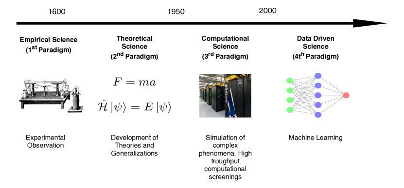
Figure 1: Different approaches to science that evolved over time, starting from empirical observation, generalizations to theories and simulation of different, complex, phenomena. The latest addition is the data-driven discovery (“fourth paradigm of science”). The supercomputer image was taken from the Oak Ridge National Laboratory.

Material science and chemistry may not be the most obvious topics for big-data science. Experiments are labor-intensive and the amount of data about materials that have been collected in the last centuries is minute compared to what Google and the likes collect every single second. However, recently the field of materials genomics has changed the landscape.¹³ High-throughput density-functional theory (DFT) calculations¹⁴ and molecular simulations¹⁵ have become routine tools to study the properties of real and even hypothetical materials. In these studies, ML is becoming more popular and widely used as a filter in the computational funnel of high-throughput screenings.¹⁶ But also to assist and guide simulations^{17, 18, 19, 20} or experiments,²¹ or to even replace them,^{22, 23} and to design new high-performing materials.²⁴

Another important factor is the prominent role patterns play in chemistry. The most famous example is Mendeleev’s periodic table, but also Pauling’s rules,²⁵ Pettifor’s maps,²⁶ and many other structure-property relationships were guided by a combination of empirical knowledge and chemical intuition. What we hope to show in this review is that ML holds the promise to discover much more complex relationships from (big) data.

We continue this section with a broad overview of the main principles of ML. This section will be followed with a more detailed and technical discussion on the different subtopics introduced in this section.

2.1 The Machine Learning Pipeline

2.1.1 Machine Learning Workflow

ML is no different from any other method in science. There are questions for which ML is an extremely powerful method to find an answer, but if one sees ML as the modern solution to any ill-posed problem one is bound to be disappointed. In section 9, we will discuss the type of questions that have been successfully addressed using ML in the contexts of synthesis and applications of porous materials.

Independent of the learning algorithm or goal, the ML workflow from materials’ data to prediction and interpretation can be divided into the following blueprint of a workflow, which also this review follows:

1. Understanding the problem: An understanding of the phenomena that need to be described is important. For example, if we are interested in methane storage in porous media, the key performance parameter is the deliverable capacity, which can be obtained directly for the experimental adsorption isotherms at a given temperature. In more general terms, an understanding of the phenomena helps us to guide the generation and transformation of the data (discussed in more detail in the next step).

   In case of the deliverable capacity we have a continuous variable and hence a regression problem, which can be more difficult to learn compared to classification problems (e.g., whether the channels in our porous material form a 1, 2 or 3-dimensional network or classifying the deliverable capacity as “high” or “low”).

   Importantly, the problem definition guides the choice of the strategies for model evaluation, selection, and interpretation (cf. section 7): In some classification cases, such as in a part of the high-throughput funnel, in which we are interested in finding the top-performing materials by down selecting materials, missing the highest-performing material is worse than doing an additional simulation for a mediocre material—this is something one should realize before building the model.

2. Generating and exploring data: Machine learning needs data to learn from. In particular, one needs to ensure that we have suitable training data. Suitable, in the sense that the data are reliable and provide sufficient coverage of the design space we would like to explore. Sometimes, suitable training data must be generated or augmented. The process of exploring a suitable data set (known as exploratory data analysis (EDA) ²⁷) and its subsequent featurization can help to understand the problem better and inform the modeling process.

   Once we have collected a data set, the next steps involve:

   1. Data selection: If the goal is to predict materials properties, which is the focus of this review, it is crucial to ensure that the available labels $\mathbf{y}$, i.e., the targets we want to predict, are consistent, and special care has to be taken when data from different sources are used. We discuss this step in more detail in section 3 and the outlook.

   2. Featurization is the process in which the structures or raw data are mapped into feature (or design) matrices $\mathbf{X}$, where one row in this matrix characterizes one material. Domain knowledge in the context of the problem we are addressing can be particularly useful in this step. For example, to select the relevant length scales (atomistic, coarse-grained, or global) or properties (electronic, geometric, or involved experimental properties). We give an overview of this process in section 4.

   3. Sampling: Often, training data are randomly selected from a large database of training points. But this is not necessarily the best choice as most likely the materials are not uniformly distributed for all possible labels we are potentially interested in. For example, one class (often the low-performing structures) might constitute the majority of the training set and the algorithm will have problems in making predictions for the minority class (which are often the most interesting cases). Special methods, e.g., farthest point sampling (FPS), have been developed to sample the design space more uniformly. In section 3.2 we discuss ways to mitigate this problem and approaches to deal with little data.

3. Learning and Prediction: In section 5 we examine several ways in which one can learn from data, and what one should consider when choosing a particular algorithm. We then describe different methods with which one can improve predictive performance and avoid overfitting (cf. section 6).
   To guide the modeling and model selection, methods for performance evaluation are needed. In section 7 we describe best practices for model evaluation and comparison.

4. Interpretation: Often it is interesting to understand what and how the model learned—e.g., to better grasp structure-property relationships or to debug ML models. ML is often seen as a black-box approach to predict numerical values with zero understanding—defeating the goal of science to understand and explain phenomena. Therefore, the need for causal models is seen as a step towards machines “that learn and think like people” (learning as model building instead of mere pattern recognition).²⁸ In section 8 we present different approaches to look into black-box models, or how to avoid them in the first place.

It is important to remember that model development is an iterative process; the understanding gained from the first model evaluations can help to understand the model better and help in refining the data, the featurization and the model architecture. For this, interpretable models can be particularly valuable.²⁹

The scope of this review is to provide guidance along this path and to highlight the caveats, but also to point to more detailed resources and useful Python packages that can be used to implement a specific step.

An excellent general overview that digs deeper into the mathematical background than this review is the “high-bias, low variance introduction to Machine Learning” by Mehta et al.⁷, recent applications of ML to materials science are covered by Schmidt et al.³⁰ But also many textbooks cover the fundamentals of machine learning; e.g., Tibshirani and Friedman³¹, Shalev-Shwartz and Ben-David³² as well as Bishop (from a more Bayesian point of view)³³ focus more on the theoretical background of statistical learning, whereas Géron provides a “how-to” for the actual implementation, also of neural network (NN) architectures, using popular Python frameworks,³⁴ which were recently reviewed by Rascka et al.³⁵

2.1.2 Machine Learning Algorithms

Step three of the workflow described in the previous section, learning and predictions, usually receives the most attention. Broadly, there are three classes, though with fuzzy boundaries, for this step, namely supervised, unsupervised and reinforcement learning. We will focus only on supervised learning in this review, and only briefly describe possible applications of the other categories and highlight good starting points to help the reader orient in the field.

Supervised Learning: Feature Matrix and Labels are Given

The most widely used flavor, which is also the focus of this review, is supervised learning. Here, one has access to features that describe a material and the corresponding labels (the property one wants to predict).

A common use case is to completely replace expensive calculations with the calculation of features that can be then fed into a model to make a prediction. A different use case can be to still perform molecular simulations—but to use ML to generate better potential energy surface (PES), e.g., using “machine learned” force fields. Another promising avenue is $\Delta$-ML in which a model is trained to predict a correction to a coarser level of theory:³⁶ One example would be to predict the correction to DFT energies to predict coupled-cluster energies.

Supervised learning can also be used as part of an active learning loop for self-driving laboratories and to efficiently optimize reaction conditions. In this review, we do not focus on this aspect—good starting points are reports from the groups around Alán Aspuru-Guzik^{37, 38, 39, 40} and Lee Cronin.^{41, 42, 43, 44}

Unsupervised Learning: Using Only the Feature Matrix

Unsupervised learning differs from supervised learning in the sense that it only uses the feature matrix and not the labels (which are often unknown when unsupervised learning is used). Unsupervised learning can help to find patterns in the data, which in turn might provide chemical insight.

Dimensionality Reduction and Clustering

The importance of unsupervised methods becomes clear when dealing with high-dimensional data which are notoriously difficult to visualize and understand (cf. section 4.1). And in fact some of the earliest applications of these techniques were to analyze^{45, 46, 47} and then speed up molecular simulations.^{48, 49} The challenge with molecular simulations is that we explore a $3N$ dimensional space, where $N$ is the number of particles. For large $N$, as it is, for example, the case for the simulation of protein dynamics, it can be hard to identify low energy states.⁴⁸ To accelerate the sampling, one can apply biasing potentials that help the simulation to move over barriers between metastable states. Typically, such potentials are constructed in terms of a small number of variables, known as collective variables—but it can be a challenge to identify what a good choice of the collective variables is when the dimensionality of the system is high. In this context, ML has been employed to lower the dimensionality of the system (cf. Figure 2 for an example of such a dimensionality reduction) and to express the collective variables in this low-dimensional space.

Figure 2: A, Three-dimensional energy landscape and B, its two-dimensional projection using sketchmap, which is a dimensionality reduction technique. The biasing potentials can now be represented in terms of sketchmap coordinates. Figure reproduced from ⁴⁸, Copyright (2012) National Academy of Sciences.

Dimensionality reduction techniques, like principal component analysis (PCA), ISOMAP, t-distributed stochastic neighbor embedding (t-SNE), self-organizing maps,^{50, 51} growing cell structures,⁵² or sketchmap,^{53, 54} can be used to do so.⁴⁸ But they can also be used for “materials cartography”,⁵⁵ i.e., to present the high-dimensional space of material properties in two dimensions to help identify patterns in big and high-dimensional data.⁵⁶ A book chapter Samudrala et al.⁵⁷ and a perspective by Ceriotti⁵⁸ give an overview of applications in materials science.

Recently, unsupervised learning—in the form of word-embeddings, which are vectors in the multidimensional “vocabulary space” that are usually used for natural language processing (NLP)—has also been used to discover chemistry in form of structure-property relationships in chemical literature. This technique could also be used to make recommendations based on the distance of a word-embedding of a compound, to the vector of a concept such as thermoelectricity in the word-embedding space.⁵⁹

Generative Models

One ultimate goal of ML is to design new materials (which recently has been also popularized as “inverse design”). Generative models, like generative adverserial networks (GANs) or variational autoencoderss (VAEs) hold the promise to do this.⁶⁰ GANs and VAEs can create new molecules,⁶¹ or probability distributions,⁶² with the desired properties on the computer.¹⁸ One example for the success of generative techniques (in combination with reinforcement learning) is the discovery of inhibitors for a kinase target implicated in fibrosis, that were discovered in 21 days on the computer and also showed promising results in experiments.⁶³ An excellent outline of the promises of generative models and their use for the design of new compounds is given by Sanchez²⁴ and Elton.⁶⁴

The interface between unsupervised and supervised learning is known as semi-supervised learning. In this setting, only some labels are known, which is often the case when labeling is expensive. This was also the case in a recent study of the group around Ceder,⁶⁵ where they attempted to classify synthesis descriptions in papers according to different categories like hydrothermal or solid-state synthesis. The initial labeling for a small subset was performed manually, but they could then use semi-supervised techniques to leverage the full datasets, i.e., also the unlabeled parts.

Reinforcement Learning: Agents Maximizing Rewards

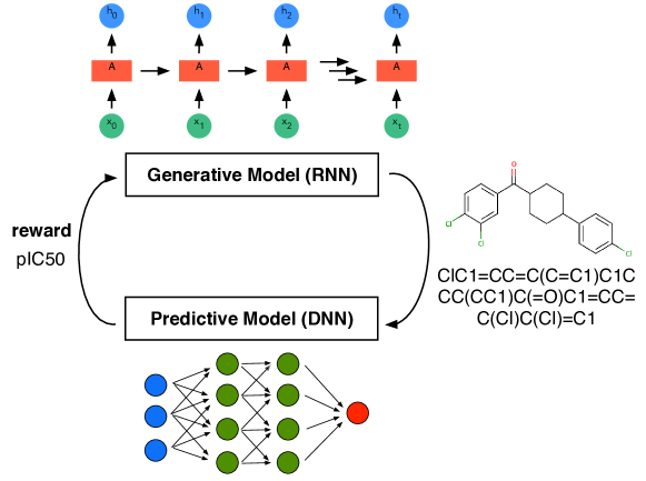
Figure 3: Reinforcement learning scheme illustrated based on the approach chosen by Popova et al.⁶⁶ for drug design. They use a RNN (cf. section 5.1.1) for the generation of SMILES strings and a deep NN for property prediction. In a first stage, both models are trained separately, and then they are used jointly to bias, using the target properties as the reward, the generation of new molecules. This example also nicely shows that the boundary between the different “flavors” of ML is fuzzy and that they are often used together.

In reinforcement learning⁶⁷ agents try to figure out the optimal sequence of actions (which is known as policy) in some environment to maximize a reward. An interesting application of this sub-field of ML in chemistry is to find the optimal reaction conditions to maximize the yield or to create structures with desired properties (cf. Figure 3).^{68, 66} Reinforcement learning has also been in the news for the superhuman performance achieved on some video games.^{69, 70} Still, it tends to require a lot of training. AlphaGo Zero, for example, needed nearly 5 million matches, requiring millions of dollars of investment in hardware and computational time.⁷¹

2.2 Theory-Guided Data Science

We are at an age in which some argue that “the end of theory” is near,⁷² but throughout this review we will find that many successful ML models are guided by physics and physical insights.^{73, 74, 75} We will see that the symmetry of the systems guides the design of the descriptors and can guide the design of the models (e.g., by decomposing the problems into sub-problems) or the choice of constraints. Sometimes, we will also encounter hybrid approaches where one component of the problem (often the local part, as locality is often an assumption for the ML models, cf. section 4.1) is solved using ML and that for example the electrostatic, long-range interaction, is added using well-known theory.

Generally, the decomposition of the problem can help to debug the model, and make the model more interpretable and physical.⁷⁶ For example, physics-guided breakdown of the target proved to be useful in the creation of a model for the equation of state of fluid methane.⁷⁷

Physical insight can also be introduced using sparsity,⁷⁸ or physics-based functional forms.⁷⁹ Constraints, introduced for example via Euler-Lagrange constrained minimization or coordinate scaling (stretching the coordinates should also stretch the density), have also proven to be successful in the development of ML learned density functionals.^{80, 81}

That physical insight can guide model development has been shown by Chmiele et al., who built a model of potential energy surfaces using forces instead of energies to respect energy conservation (also, the force is a quantity that is well-defined for atoms, whereas the energy is only defined for the full system).^{82, 83}

This paradigm of incorporating domain knowledge into the ML workflow is also known as theory-guided data science.^{84, 85} Theory-guided data science can help to get the right answers for the right reasons, and we will revisit it in every chapter of this review.

2.3 The Scientific Method in Machine Learning: Strong Inference and Multiple Models

Throughout this review we will encounter the method of strong inference,^{86, 87} i.e., the need for alternative hypotheses, or more generally the integral role of critical thinking, at different places—mostly in the later stages of the ML pipeline when one analyzes a model. The idea here is to always pursue multiple alternative hypotheses that could explain the performance of a model: Is the improved performance really because of a more complex architecture or rather due to better hyperparameter optimization (cf. ablation testing in section 7.8.1) or does the model really learn sensible chemical relationships or could we achieve similar performance with random labels (cf. randomization tests as discussed in section 7.9^{88, 89})?

ML comes with many opportunities, but also many pitfalls. In the following, we review the details of the supervised ML workflow to aid the use of ML for the progress of our field.

3 Selecting the Data: Dealing with Little, Imbalanced and Non-Representative Data

The first, but most important step in ML is to generate good training data.⁹⁰ This is also captured in the “garbage in garbage out” saying among ML practitioners. Data matters more than algorithms.^{6, 91} In this section, we will mostly focus on the rows of the feature matrix, $\mathbf{X}$, and discuss the columns of it, the descriptors, in the next section.

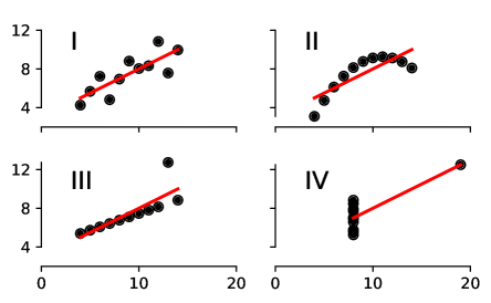
Figure 4: Anscombe’s quartet shows the importance of visualization.⁹² The four datasets have the same mean (7.50), standard deviation (1.94), and regression line, but still look completely different.

That the selection of suitable data can be far from trivial is illustrated with Anscombe’s quartet (cf. Figure 4).⁹² In this archetypal example four different distributions, with distinct graphs, have the same statistics, e.g., due to single high-leverage points. This example emphasizes the notion in ML that statistics can be deceiving, and why in ML so much emphasis is placed on the visualization of the data sets.

3.1 Limitations of Hypothetical Databases

Hypothetical databases of COFs, MOFs and zeolites have become popular and are frequently used as a training set for ML models—mostly because they are the largest self-consistent data sources that are available in this field. But due to the way in which the databases are constructed they can only cover a limited part of the design space (as one uses a finite, small, numbers of linkers and nodes)—which is also not necessarily representative of the “real world”.

The problem of idealized models and hypothetical structures is even more pronounced for materials with unconventional electronic properties. Many features that favor topological materials, which are materials with special shape of their electronic bands due to the symmetries of the atom positions, work against stability. For example, creating a topological insulator (which is insulating in the bulk, but conductive on the surface) involves moving electrons into antibonding orbitals, which weakens the lattice.⁹³ Also, in the real world one often has to deal with defects and kinetic phenomena—real materials are often non-equilibrium structures^{93, 94}—while most databases assume ideal crystal structures.

3.2 Sampling to Improve Predictive Performance

A widespread technique in ML is to randomly split the all available data into a training and a test set. But this is not necessarily the best approach as random sampling might not sample some sparsely populated regions of the chemical space. A more reasonable sampling approach would cover as much of the chemical space as feasible to construct a maximally informed training set. This is especially important when one wants to minimize the number of training points. Limiting the number of training points can be reasonable or even essential when the featurization or labeling is expensive e.g. when it involves experiment or ab initio calculations. But it can also be necessary for computational reasons as in the case of kernel methods (cf. section 5.2.2), for which the data needs to be kept in memory and for which the computational cost scales cubically with the number of training points.

3.2.1 Diverse Set Selection

(Greedy) Farthest Point Sampling

Instead of randomly selecting training points, one can try to create a maximally diverse dataset to ensure a more uniform sampling of the design space and to avoid redundancy. Creating such as dataset, in which the distances between the chosen data points are maximized, is known as the maximum diversity problem (MDP).⁹⁵ Unfortunately, the MDP, is of factorial computational cost, and hence becomes computationally prohibitive for large datasets.^{96, 97, 98} Therefore, in practice, one usually uses a greedy algorithm to perform FPS. Those algorithms add points for which the minimum distance to the already chosen points is maximal (i.e., using the max-min criterion, this sampling approach is also known as Kennard-Stone sampling, cf. pseudocode in Listing 1).

This FPS is also a key to the work by Moosavi et al.²¹, in which they use a diverse set of initial reaction conditions, most of which will yield to failed reactions, to build their model for reaction condition prediction.

Listing 1: Pseudocode for the greedy implementation of a FPS scheme. The initialization could also be to choose a point that is maximally distant from the center or using the two most separated points, as in the original Kennard-Stone framework.

⬇

1# initialize by choosing a random point from the dataset p

2Q =[]

3Q.append(random.choice(p))

4

5# perform the greedy search

6while len(Q) < k:

7 # select the point with the maximal minimal distance

8 new_point_index = argmax(min(d(p, Q)))

9 # add point to the selected subset

10 Q.append(p[new_point_index])

11 # remove point from the old set

12 p.remove(new_point_index)

Design of Experiments

The efficient exploration is also the main goal of most design of experiment (DoE) methods,^{99, 100} which in chemistry have been widely used for reaction condition or process optimization,^{101, 102, 103, 104} where the task is to understand the relationship between input variables (temperature, reaction time, …) and the reaction outcome in the least time and effort possible. But they also have been used in computer science to generate good initial guesses for computer codes.^{105, 106}

If our goal is to perform reaction condition prediction, the use of DoE techniques can be a good starting point to get an initial training set that covers the design space. Similarly, they can also be a good starting point if we want to build a model that correlates polymer building blocks with the properties of the polymer: since also in this case, we want to make sure that we sample all relevant combinations of building blocks efficiently. The most trivial approach in DoE is to use a full-factorial design in which the combination of all factors in all possible levels (e.g., all relevant temperatures and reaction times) are tested. But this can easily lead to a combinatorial problem. As we discussed in section 3.2.1, one could cover the design space using FPS. But the greedy FPS also has some properties that might not be desirable in all cases.¹⁰⁷ For instance, it tends to preferentially select points that lie at the boundaries of design space. Also, one might prefer that the samples are equally spaced along the different dimensions.

Different classical DoE techniques can help to overcome these issues.¹⁰⁷ In latin hypercube sampling (LHS) the range of each variable is binned in equally spaced intervals and the data is randomly sampled from each of these intervals—but in this way, some regions of space might remain unexplored. For this reason, the max-min-LHS has been developed in which evenly spread samples are selected from LHS samples using the max-min criterion.

Alternative Techniques

An alternative for the selection of a good set of training points can be the use of special matrix decompositions. CUR is a low-rank matrix decomposition into matrices of actual columns (C) and rows (R) of the original matrix, which main advantage over other matrix decompositions, such as PCA, is that the decomposition is much more interpretable due to use of actual columns and rows of the original matrix.¹⁰⁸ In the case of PCA, which builds linear combinations of features, one would have to analyze the loadings of the principal components to get an understanding. In contrast, the CUR algorithm selects the columns (features) and rows (structures) which have the highest influence on the low-rank fit of the matrix. And selecting structures with high statistical leverage is what we aim for in diverse set selection. Bernstein et al. found that the use of CUR to select the most relevant structures was the key for their self-guided learning of PES, in which a ML force-field is built in an automated fashion.¹⁰⁹

Further, also D-optimal design algorithms have been put to use, in which samples are selected that maximize the $\|\mathbf{X}^{T}\mathbf{X}\|$ matrix, where $\mathbf{X}$ is the information matrix (in some references it is also called dispersion matrix) which contains the model coefficients in the columns and the different examples in the rows.^{110, 111, 112} Since it requires the model coefficients, it was mostly used with multivariate linear regression models in cheminformatics.

Moreover, other unsupervised learning approaches such as self-organizing maps,⁵⁰ $k$ nearest neighbor ($k$NN),¹¹³ sphere exclusion¹¹⁴ or hierarchical clustering^{115, 116} have been used, though mostly for cheminformatics applications.¹¹⁷

Sampling Configurations

For fitting of models for potential energy surfaces, non-equilibrium configurations are needed. Here, it can be practical to avoid arbitrarily sampling from trajectories of molecular simulations as consecutive frames are usually highly correlated. To avoid this, normal mode sampling, where the atomic positions are displaced along randomly scaled normal modes, has been suggested to generate out-of-equilibrium chemical environments and has been successfully applied in the training of the ANI-1 potential.¹¹⁸ Similarly, binning procedures, where e.g., the amplitude of the force in images of a trajectory is binned have been proposed. When generating the training data, one can then sample from all bins (like in LHS).⁸³

Still, one needs to remember that the usage of rational sampling techniques does not necessarily improve the predictive performance on a brand-new dataset which might have a different underlying distribution.¹¹⁹ For example, hypothetical databases of COFs contain mainly large pore structures, which are not as frequent in experimental structures. Training a model on a diverse set of hypothetical COFs will hence not guarantee that our model can predict properties of experimental structures, which might be largely non-porous.

An alternative to rationally chosen (e.g., using DoE techniques or FPS), and hence static, datasets is to let the model (actively) decide which data to use. We discuss this active learning technique next.

3.3 Active Learning

An alternative to using static training sets, which are assembled before training, is to let the machine decide which data are most effective to improve the model at its current state.¹²⁰ This is known as active learning.¹²¹ And it is especially valuable in cases where the generation of training data is expensive, such as for experimental data or high-accuracy quantum chemical calculations where a simple “Edisonian” approach, in which we create a large library of reference data by brute force, might not be feasible.

Similar ideas, like adding quantum-mechanical data to a force field when needed, have already been used in molecular dynamics simulations before they became widespread among the ML practitioners in materials science and chemistry.^{122, 123}

One of the ways to determine where the current model is ambiguous, i.e., to decide when new data is useful, is to use an ensemble of models (which is also known as “query by committee”).^{124, 125} The idea here is to train an ensemble of models, which are slightly different and hence will likely give different, wrong, answers if the model is used outside its domain of applicability (cf. section 7.6); but the answers will tend to agree mostly when the model is used within the domain of applicability.

Another form of uncertainty sampling is to use a model that can directly output a probability estimate—like the width of the posterior (target) distribution of a Gaussian process (cf. section 5.2.3 for more details). One can then add training points to the space where the distribution is wide and the model is uncertain.¹²⁶

Botu and Ramprasad reported a simpler strategy, which is related to the concept of the domain of applicability, which we will discuss below (cf. section 7.6). The decision if a configuration needs new training data is not made based on an uncertainty measure but merely by using the distance of the fingerprints to the already observed ones.¹²⁷ Active learning is closely linked to Bayesian hyperparameter optimization (cf. section 6.1) and self-driving laboratories, as they have the goal to choose experiments in the most efficient way, where active learning tries to choose data in the most efficient way.^{128, 129}

3.4 Dealing With Little Data

Often, one can use tricks to artificially enlarge the dataset to improve model performance. But these tricks generally require some domain knowledge to decide which transformations are applicable to the problem, i.e. which invariances exist. For example, if we train a force field for a porous crystal, one can use the symmetry of the crystal to generate configurations with equivalent energies (which would be a redundant operation when one uses descriptors that already respect this symmetry). For image data, like steel microstructures¹³⁰ or 2D diffraction patterns,¹³¹ several techniques have been developed, which include to randomly rotate, flip or mirror the image which is, for example, implemented in the ImageDataGenerator module of the keras Python package. Notably, there is also effort to automate the augmentation process and promising results have been reported for images.¹³² However, data augmentation always relies on assumptions about the equivariances and invariances of the data, wherefore it is difficult to develop general rules for any type of dataset.

Still, the addition of Gaussian noise is a method that can be applied on most datasets.¹³³ This works effectively as data augmentation if the data is presented multiple times to the model (e.g., in NNs where one has multiple forward and backward passes of the data through the network). By the addition of random noise, the model will then see a slightly different example upon each pass of the data. The addition of noise also acts as “smoother”, which we will explore in more detail when we discuss regularization in section 6.2.1.

Oviedo et al. reported the impact data augmentation can have in materials science. Thin-film x-ray diffraction (XRD) patterns are often distorted and shifted due to strain or lattice contraction or expansion. Also, the orientations of the grains are not randomized, as they are in a powder, and some reflexes will have an increased intensity depending on the orientation of the film. For this reason, conventional simulations cannot be used to form a training set for a ML model to predict the space group based on the diffraction pattern. To combat the data scarcity problem, the authors expanded the training set, generated by simulating diffraction patterns from a crystal structure database, by taking data from the training set and by scaling, deleting or shifting of reflexes in the patterns. In this way, the authors generated new training data that correspond to the typically experimental distortions.¹³⁴ A similar approach was also chosen by Wang et al. who built a convolutional neural network (CNN) to identify MOFs based on their x-ray powder diffraction (XRPD) patterns. Wang et al. predicted the patterns for MOFs in the Cambridge Structure Database (CSD) and then augmented their dataset by creating new patterns by merging the main peaks of the predicted patterns with (shuffled) noise from pattern they measured in their own lab.¹³⁵

Sometimes, data augmentation techniques have also been used to solve non-uniqueness or invariance problems. The Chemception model is a CNN, inspired by models for image recognition, that is trained to predict chemical properties based on images of molecular drawings.¹³⁶ The prediction should, of course, not depend on the relative orientation of the molecule in the drawing. For this reason, the authors applied augmentation methods such as rotations. Interestingly, many image augmentation techniques also use cropping. However, the local information density in drawings of molecules is higher than in usual images and hence losing a part of the image would be a more significant problem.

Another issue is that not all datasets are unique. For example, if one uses (non-canonical) SMILES strings to describe molecules, one has to realize that they are not unique. Therefore, Bjerrum trained this model on all possible SMILES string for a molecule and obtained a dataset that was 130 times bigger than the original dataset.¹³⁷ This idea was also used for the Coulomb matrix, a popular descriptor that encodes the structure by capturing all pairwise Coulomb terms, based on the nuclear charges, in a matrix (cf. section 4.2.2). Without additional steps, this representation is not permutation invariant (swapping rows or columns does not change the molecule but would change the representation). Montavon used an augmented dataset and in which they mapped each molecule to a set of randomly sorted Coulomb matrices and could improve upon other techniques of enforcing permutation symmetry—likely due to the increased dataset size.¹³⁸

But also simple physical heuristics can help if there is only little data to learn from. Rhone et al. used ML to predict the outcome of reactions in heterogeneous catalysis, where only little curated data is available.¹³⁹ Hence, they aided their model with a reaction tree and chose the prediction of the model that is closest to a point in the reaction tree (and hence a chemically meaningful reaction). Moreover, they also added heuristics like conservation rules and penalties for some transformations (e.g., based on the difference of heavy atoms in educts and products) to support the model.

Another promising avenue are multitask learning approaches where a model, like a deep neural networks (DNN), is trained to predict several properties. The intuition here is to capture the implicit information in the relationship between the multimodal variables.^{140, 141} Closely related to this are transfer learning approaches (cf. section 10.3), where on trains a model on a large dataset and then “refines” the weights of the model using a smaller dataset.¹⁴² Again, this approach is a well-established practice in the “mainstream” ML community.

Given the importance of the data scarcity problem, there is a lot of ongoing effort in developing alternative solutions to combat this challenge, many of which build on encoding-decoding architectures. Generative models like GANs or VAE can be used to create new examples by learning how to generate underlying distribution of the data.¹⁴³

Some problems may also be suitable for so-called one-shot learning approaches.^{144, 76, 145} In the field of image recognition, the problem of correctly classifying an image after seeing only one training example for this class (e.g. correctly assigning names to images of persons after having seen only one image for each person) has received a lot of interest. Supposedly, because this is what humans are able to do—but machines are not, at least not in the “usual” classification setting.²⁸

One- or few-shot learning is based on learning a so-called attention mechanism.¹⁴⁶ Upon inference, the attention mechanism, which is distance measure to the memory, can be exploited to compare the new example to all training points and express the prediction as a linear combination of all labels in the support set.¹⁴⁷ One approach to do this is Siamese learning, using a NN that takes two inputs and then learns an attention mechanism. This has also been used, in a refined formulation, by Pande and co-workers to classify the activity of small molecules on different assays for pharmaceutical activity.¹⁴⁸ Such techniques are especially appealing for problems where only little data is available.

Still, one always should remember that there is no absolute number that defines what “little data” is. This number depends on the problem, the model, and the featurization. But it can be estimated using learning curves, in which one plots the error of the model against the number of training points (cf. section 7).

3.5 Dealing With Imbalanced Data Labels

Often, data is imbalanced, meaning that different classes which we attempt to predict (e.g. “stable” and “unstable”, or “low performing” and “high performing”) do not have the same number of examples in our training set. Balachandran et al. faced this challenge when they tried to predict compounds that break spatial inversion symmetry, and hence could be interesting for e.g. their piezoelectric properties.¹⁴⁹ They found that one symmetry group was misclassified to $100\text{\,}\mathrm{\char 37\relax}$ due to imbalanced data. To remedy this problem, they used an oversampling technique, which we will briefly discuss next.

Oversampling, which means adding points to the underrepresented class, is one of the most widely used approaches to deal with imbalanced data. The opposite approach is undersampling, in which instances of the majority class are removed. Since random oversampling can cause overfitting (due to replication of training points) and undersampling can lead to poorer predictive performance (as training points are eliminated) both strategies have been refined by means of interpolative procedures.¹⁵⁰

The synthetic minority oversampling technique (SMOTE) for example, creates new (synthetic) data for the minority class by randomly selecting a point on the vector connecting a data point from the minority class with one of its nearest neighbors. In SMOTE, each point in the minority class is treated equally—which might not be ideal since one would expect that examples close to class boundaries are more likely to be misclassified. Borderline-SMOTE and adaptive synthetic oversampling (ADASYN) try to improve on this point. In a similar vein, it can also be easier to learn clear classification rules when so-called Tomek links¹⁵¹ are deleted. Tomek links are pairs of two points from different classes for which the distance to the example from the alternative class is smaller than to any other example from their class.

Still, care needs to be taken in the case of very imbalanced data in which algorithms can have difficulties to recognize class structures. In this case over- or undersampling can even deteriorate the performance.¹⁵²

A useful Python package to address data imbalance problems is imbalanced-learn, which implements all the methods we mentioned and which are analyzed in more detail in a review by He and Garcia.¹⁵⁰ There they also discuss cost-sensitive techniques. In these approaches, a cost matrix is used to describe a higher penalty for misclassifying examples from a certain class—which can be an alternative strategy to deal with imbalanced data.¹⁵⁰ Importantly, oversampling techniques should only be applied—as all data transformations—after the split into training and test sets.

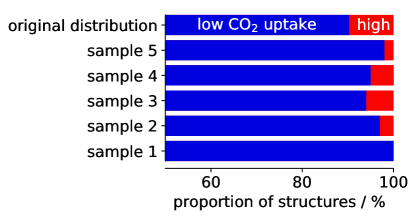
Figure 5: Example for the importance of stratification. For this example, we use a threshold of $2.5\text{\,}\mathrm{m}\mathrm{mol}\,\ce{CO2}\mathrm{/}\mathrm{g}$ to group structures in low and high performing materials, which is slightly higher than the threshold chosen by Boyd et al.¹³ Then, we randomly draw 100 structures and can observe that the class distribution gets distorted—sometimes we do not have any high performing materials in our sample. Stratification can be used to remedy this effect.

In any case, it is also advisable to use stratified sampling which ensures that the class proportions in the training set are equal to the ones in the test set. An example of the influence of stratified sampling is shown in Figure 5 where we contrast the random with the stratified splitting of structures from the database of Boyd et al.¹³

4 What To Learn From: Translating Structures Into Feature Vectors

After having reviewed the rows of the feature matrix, we now focus on the columns and discuss ways to generate those columns (descriptors), and how to select the best ones (as more is not always better in the case of feature columns). The possibilities for structural descriptors are so vast that it is impossible to give a comprehensive overview. Especially since there is no silver bullet and the performance of descriptors depends on the problem and the learning setting. In some cases, local fingerprints based on symmetry functions might be more appropriate, e.g., for potential energy surfaces, whereas in other cases, where structure-property insights are needed, higher-level features such as pore shapes and sizes can be more instructive.

An important distinction of NNs compared to classical ML models, like kernel methods (cf. section 5.2.2) is that NNs can perform representation learning, i.e., the need for highly engineered structural descriptors is less pronounced than for “classical” learners as NN can learn their own features from unstructured data. Therefore, one will find NN models that directly use the positions and the atomic charges whereas such an approach is deemed to fail with classical ML models, like kernel ridge regression (KRR), that rely on structured data. The representation learning of NNs can potentially leverage regularities in the data that cannot be described with classical descriptors—but it only works with large amounts of data. We will discuss this in more detail when we revisit special NN architectures in section 5.1.1.

The quest for good structural descriptors is not new. Cheminformatics researchers tried to devise strategies to describe structures, e.g., to determine whether a compound has already been deposited on the chemical abstract services (CAS) database, which led to the development of Morgan fingerprints.¹⁵³ Also the demand for quantitative structure activity relationship (QSAR) in drug development led to the development of a range of descriptors that are often highly optimized for a specific application (also because simple linear models have been used) as well as heuristics (e.g., Lipinkski’s rule of five¹⁵⁴). But also fingerprints (e.g., Daylight fingerprints)—i.e., representations of the molecular graphs have been developed. We will not discuss them in detail in this review as most of them are not directly applicable to solid-state systems.^{155, 156} Still, one needs to note that for the description of MOFs one needs to combine information about organic molecules (linkers), metal centers, and the framework topologies wherefore not all standard featurization approaches are ideally suited for MOFs. Therefore, molecular fingerprints can still be interesting to encode the chemistry of the linkers in MOFs, which can be important for electronic properties or more complex gas adsorption phenomena (e.g., involving CO2, H2O).

Figure 6: Building principle of the MOFid and MOFkey identifiers for HKUST-1. Bucior et al. use a SMILES derived format in the MOFid and whereas the MOFkey is inspired by the InChIkey format, which is a hashed version of the InChi fingerprint, which is more standardized than SMILES. Figure adopted from Bucior et al,¹⁵⁷

A decomposition of MOFs into the building blocks and encoding of the linker using SMILES was proposed in the MOFid scheme from Bucior et al. (cf. Figure 6).¹⁵⁷ This scheme is especially interesting to generate unique names for MOFs and in this way to simplify data-mining efforts. For example, Park et al. had to use a six-step process to identify whether a string represents the name of a MOF in their text-mining effort,¹⁵⁸ and then one still has to cope with non-uniqueness problems (e.g., Cu-BTC vs. HKUST-1). One main problem of such fingerprinting approaches for MOFs is that they require the assignment of bonds and bond orders, which is not trivial for solid structures,¹⁵⁹ and especially for experimental structures that might contain disorder or incorrect protonation.

The most popular fingerprints for molecular systems are implemented and documented in libraries like RDKit,¹⁶⁰ PaDEL¹⁶¹ or Mordred.¹⁶² For a more detailed introduction into descriptors for molecules we can recommend a review by Warr¹⁶³ and the “Deep Learning for the Life Sciences” book,¹⁶⁴ which details on how to build ML systems for molecules.

4.1 Descriptors

There are several requirements that an ideal descriptor should fulfill to be suitable for ML:^{165, 166}

• A descriptor should be invariant with respect to transformations that preserve the target property (cf. Figure 7).

  

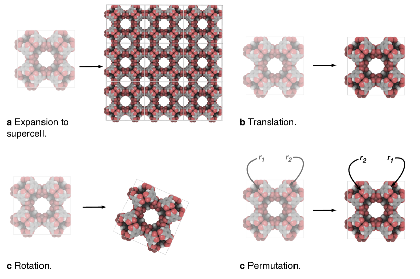
  Figure 7: Illustration of transformations of crystal structures to which an ideal descriptor should be invariant. Structures drawn with iRASPA.¹⁶⁷

  For crystal structures, this means that the representations should respect periodicity, translational, rotational and permutation symmetry (i.e., the numbering of the atoms in the fingerprint should not influence the prediction). Similarly, one would want equivariances to be conserved. Equivariant functions transform in the same way as their arguments, as it is, for example, the case for the tensorial properties like the force (negative gradient of energy) or the dipole moment, which both translate the same way as the positions.^{168, 169}

  Respecting those symmetries is important from a physics perspective as (continuous) symmetries are generally linked to a conserved property (cf. Noether’s theorem, e.g., rotational invariance corresponds to conservation of angular momentum). Conceptually, this is different from classical force field design where one usually focuses on correct asymptotic behavior. In ML, the intuition is to rather use symmetries to preclude completely nonphysical interactions.

  As discussed above, one could in principle also attempt to include those symmetries using data augmentation techniques, but it is often more robust and efficient to “hard-code” them on the level of the descriptor. Notably, the introduction of the invariances on the descriptor level also removes alignment problems, when one would like to compare two systems.

• A descriptor should be unique (i.e., non-degenerate). This means that each structure should be characterized by one unique descriptor and that different structures should not share the same descriptor. When this is not the case, the model will produce prediction errors that cannot be removed with the addition of data.¹⁷⁰ Von Lilienfeld et al. nicely illustrate this in analogy to the proof of the first Hohenberg-Kohn theorem trough reductio ad absurdum.¹⁷¹ This uniqueness is automatically the case for invertible descriptors.

• A descriptor should allow for (cross-element) generalization. Ideally, one does not want to be limited in system size or system composition. Fixed vector or matrix descriptors, like the Coulomb matrix (see section 4.2.2), can only represent systems smaller or equal to the dimensionality of the descriptor. Also, one sometimes finds that the linker type¹⁷² or the monomer type is used as a feature. Obviously, such an approach does not allow for generalization to new linkers or monomer types.

  The cross-element generalization is typically not possible if different atom types are encoded as being orthogonal (e.g., by using a separate NN for each atom type in a high-dimensional neural network potential (HDNNP) or by grouping interactions by the atomic numbers, e.g., bag of bonds (BoB), partial radial distribution function (RDF)). To introduce generalizability across atom types one needs to use descriptors that allow for a chemically reasonable measure of similarity between atom types (and trends in the periodic table). What an appropriate measure of similarity is depends on the task at hand, but an example for a descriptor that can be relevant for chemical reactivity or electronic properties is the electronegativity.

• A descriptor should be efficient to calculate. The cardinal reason for using supervised ML is to make simulations more efficient or to avoid expensive experiments or calculations. If the descriptors are expensive to compute, ML no longer fulfills this objective and there is no reason to add a potential error source.

• A descriptor should be continuous: For differentiability, which is needed to calculate, e.g., forces, and for some materials design applications⁶¹ it is desirable to have continuous descriptors. If one aims to use the force in the loss function (force-matching) of a gradient descent algorithm, at least second order differentiability is needed. This is not given for many of the descriptors which we will discuss below (like global features as statistics of elemental properties) and is one of the main distinctions of the symmetry functions from the other, often not localized, tabular descriptors which we will discuss.

Before we discuss some examples in more detail, we will review some principles that we should keep in mind when designing the columns of the feature matrix.

The Curse of Dimensionality

One of the main paradigms that guide the development of materials descriptors is the so-called curse of dimensionality, which describes that it is often hard to find decision boundaries in a high-dimensional space as the data often no longer covers the space. For example, in 100 dimensions nearly the full edge length is needed to capture $10\text{\,}\mathrm{\char 37\relax}$ of the total volume of the 100-dimensional hypercube (cf. Figure 8). This is also known as empty space phenomenon, and describes that similarity-based reasoning can fail in high dimensions given that also the nearest neighbors are no longer close in such high-dimensional spaces.⁹⁰

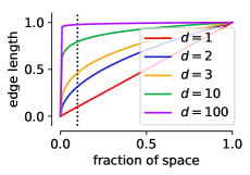
Figure 8: Illustration of the empty space phenomenon (the curse of dimensionality). For this illustration we consider the data to be uniformly distributed in a $d$ dimensional unit cube. The edge length of a hypercube corresponding to a fraction $q$ of the total volume is $q^{1/d}$, which we plotted here for different $d$. The dotted line in the figure represents $10\text{\,}\mathrm{\char 37\relax}$ of the volume, for which we would nearly need to consider the full edge length in 100-dimensional space. This means that locality is lost in high dimensions, which can be problematic for algorithms that use the local neighborhood for their reasoning.

Often, this is also discussed in terms of Occam’s razor: “Simpler solutions are more likely to be correct than complex ones.” This not only reflects that learning in high-dimensional space brings its own problems but also that simplicity, which might be another way of asking of explainability, for itself is a value (due to its aesthetics) we should strive for.¹⁷³ More formally, this is related to the minimum descriptor length principle¹⁷⁴ which views learning as a compression process and in which the best model is the smallest one in terms of itself and the data (this idea is rooted in Solomonoff’s general theory of inference¹⁷⁵).^{176, 177}

Chemical Locality Assumption

Many descriptors that we discuss below are based on the assumption of chemical locality, meaning that the total property of a compound can be decomposed into a sum of contributions of local (atom-centered) environments:

$$\text{property}(\text{descriptor})=\sum_{i}^{\text{atoms}}\text{model}_{i}\left(\text{descriptor}_{i}\right).$$ (1)

This approximation (cf. eq. 1) is often used in models describing the PES.

The locality approximation is usually justified based on the nearsightedness principle of electronic matter, which says that a perturbation at a distance has little influence on the local density.¹⁷⁸ And this “nearsighted” approach also guided the development of many-body potentials like embedded atom methods, linear-scaling DFT methods or other coarse-grained models in the past (also here the system is divided into subsystems).^{179, 180}

The division into subsystems can also be a feat for training of ML models, as one can learn on fragments to predict larger systems, as it has been done for example for a HDNNP for MOF-5.¹²⁵ Also, this approach makes it easier to incorporate size extensivity, i.e., to ensure that the energy of a system composed of the subsystems $A+B$ is indeed the sum of the energies of $A$ and $B$.¹⁸¹

But such an approach might be less suited for cases like gas adsorption where both the local chemical environment (especially for chemisorption) but also the pore shape, size, and accessibility play a role—i.e., one wants pore-centered descriptors rather than atom-centered descriptors. For this case global, “farsighted”, descriptors of the pore size and shape, like pore limiting diameters, accessible surface areas,^{182, 183, 184} or persistent homology fingerprints,¹⁸⁵ can be better suited. This is important to keep in mind as target similarity, i.e., how good we can the property of interest (e.g., the PES or the gas adsorption properties), is one of the main contributions to the error of ML models.¹⁸⁶ Also, one should be aware that typically cutoffs of $6\text{\,}\mathrm{\SIUnitSymbolAngstrom}$ around an atom are used to define the local chemical environments. In some systems, the physics of the phenomenon is, however, dominated by long-range behavior¹⁸⁷ that cannot be described within the locality approximation. Correctly describing such long-range effects is one of the main challenges of ongoing research.¹⁸⁸

Importantly, a model that assumes atom-centred descriptors is invariant to the order of the inputs (permutational invariance).¹⁸⁹ Interestingly, classical force fields do not show this property. The interactions are defined on a bond graph and the exchange of an atom pair can change the energy.^{168, 190}

4.2 An Overview of the Descriptor Landscape

In Figure 9 we show an overview of the space of material descriptors. We will distinct two main classes of descriptors; local ones, that only describe the local (chemical) environment and global ones which describe the full structures at once.

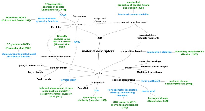
Figure 9: Non-exhaustive overview over the landscape of descriptors for solids. In blue, we highlighted descriptors for which we are aware of an application in the field of porous materials, for which we give an example in green.

Nearly as vast as the descriptor landscape is the choice of tools that are available to calculate these descriptors. Some notable developments are matminer package,¹⁹¹ which is written in Python, the DSCribe package, which has a Python interface, but where the computationally expensive routines are written in C/C++ and AMP, which also has a Python interface and where the expensive fingerprinting can be performed in Fortran.¹⁹² The von Lilienfeld group is currently also implementing efficient Fortran routines in their QML package.¹⁹³ Other packages like CatLearn,¹⁹⁴ which has also functionalities for surfaces, or QUIP,¹⁹⁵ aenet¹⁹⁶ and simple-nn¹⁹⁷, ai4materials¹⁹⁸ also contain functions for fingerprinting of solid systems. For the calculation of features based on elemental properties, i.e., statistics based on the chemical composition, the Magpie package is frequently used.¹⁹⁹

General Theme of Local and Global Fingerprints

In the following, we will also see that many fingerprinting approaches are just a variation of the same theme, namely many-body correlation functions, which can be expressed in Dirac notation as

$$\braket{\mathbf{r}}{\chi_{j}^{(1)}}=\sum_{i}\,g^{(2)}(\mathbf{r}-\mathbf{r}_{ij})\ket{\alpha_{i}}.$$ (2)

This shows that the abstract atomic configuration $\ket{\chi_{j}^{(v)}}$, in terms of the $(v+1)$-body correlation, can be described with a cross-correlation function ($g^{(2)}$ being equivalent to the radial distribution function) and information about the elemental identity of atom $i$, $\ket{\alpha_{i}}$ (see Figure 10). And it also already indicates why the term “symmetry functions” is often used for functions of this type. Descriptors based on eq. 2 are said to be symmetrized, e.g., invariant to translations of the entire structure (symmetrically equivalent positions will give rise to the same fingerprint).

Some fingerprints take into account higher orders of correlations (like triples in the bispectrum) but the idea behind most of them is the same—they are just projected onto a different basis (e.g., spherical harmonics, $\bra{nlm}$, instead of the Cartesian basis $\bra{\mathbf{r}}$).^{200, 201} Notably, it was recently shown that also three-body descriptors do not uniquely specify the environment of an atom, but Pozdnyakov et al. also showed that in combination with many neighbors, such degeneracies can often be lifted.²⁰²

Different flavors of correlation functions are used for both local and global descriptors, and the different flavors might converge differently with respect to the addition of terms in the many-body expansion (going from two-body to the inclusion of three-body interactions and so on).²⁰³ Local descriptors are usually derived by multiplying a version (projection onto some basis) of the many-body correlation function with a smooth cutoff function such as

$$f_{c}\left(r_{ij}\right)=\left\{\begin{array}[]{ll}0.5\times\left[\cos\left(\frac{\pi r_{ij}}{r_{c}}\right)+1\right]&\text{ for }r_{ij}\leq r_{c}\\ 0&\text{ for }r_{ij}>r_{c}\end{array}\right.$$ (3)

where $r_{\text{cut}}$ is the cutoff radius, which determines the set of $i$ the summation in equation 2 runs over.

We will start our discussion with local descriptors that use such a cutoff function (cf. eq. 3) and which are usually employed when atomic resolution is needed.

In some cases, especially when only the nearest neighbors should be considered, Voronoi tessellations are used to assign which atoms from the environment should be included in the calculation of the fingerprint. This approach is based on the nearest neighbor assignment method that was put forward by O’Keeffe.²⁰⁴

4.2.1 Local Descriptors

Instantaneous Correlation Functions via Cutoff Functions

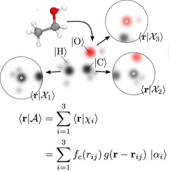
Figure 10: Illustration of the concept of featurization using symmetry functions. There are atom centered local environments that we can represent with abstract kets $\ket{\chi}$, expressed in the basis of Cartesian coordinates $\bra{\mathbf{r}}$. The Figure is a modified version of an illustration from Ceriotti and co-workers.²⁰⁰

For the training of models for PES, flavors of instantaneous correlation functions have become the most popular choices, and are often used with kernel methods (cf. section 5.2.2) or HDNNP (cf. section 5.1.1).

The archetypal examples of this type are the atom-centered symmetry functions suggested by Behler and Parinello, where the two-body term has the following form

$$G_{i}^{2}=\sum_{j\neq i}^{\text{all}}\exp\left[-\eta\left(r_{ij}-R_{s}\right)^{2}\right]f_{c}\left(r_{ij}\right),$$ (4)

which is a sum of Gaussians and the number of neighbors that are taken into account in the summation is determined by the cutoff function $f_{c}$ (cf. eq. 3). Behler and Parinello also suggest a three-order term, which takes all the internal angles for triplets of atoms, $\theta_{ijk}$, into account. This featurization approach has been the driver of the development of many HDNNPs (cf. section 5.1.1).

One should note that these fingerprints contain a set of hyperparameters that should be optimized, like the shift $R_{s}$ or the width of the Gaussian $\eta$, for which usually at set of different values is used to fingerprint the environment. Also, similar to molecular simulations, the cutoff $r_{c}$ is a parameter that should be carefully set to ensure that the results are converged.

Fingerprints of this type (cf. eq. 2) are translational invariant, because they only depend on internal coordinates and rotational invariant, because they only depend on internal angles (in case of the $v=3$ correlation). The permutation invariance is due to the summation (which does not depend on the order) over all neighbors $i$, in eq. 4 (and also in the locality approximation itself, cf. eq. 1).

An alternative approach for fingerprinting in terms of symmetry functions has been put forward by Csányi and co-workers.²⁰⁵ They started by proposing the bispectrum descriptor which is based on expanding the atomic density distribution (with Dirac delta functions for $g$ in equation 2) in spherical harmonics. This allows, as advantage over the Behler-Parinello symmetry functions, for systematic improvements via the addition of spherical harmonics.

This corresponds to a projection of the atomic density onto a four-dimensional sphere and representing the location in terms of four-dimensional spherical harmonics.^{203, 206} This descriptor was improved with the smooth overlap of atomic positions (SOAP) methodology, which is a smooth similarity measure of local environments (covariance kernel, which we will discuss in section 5.2.2) by writing $g(r)$ in eq. 2 using atom-centered Gaussians as expansions with sharp features (Dirac delta functions in the bispectrum) are slowly converging.

Given that SOAP is a kernel, this descriptor found the most application in kernel-based learning (which we will discuss below in more detail, cf. section 5.2.2), as it directly defines a similarity measure between environments (overlap between the smooth densities), which has recently extended to tensorial properties.²⁰⁷ This enabled Wilkins et al. to create models for the polarizability of molecules.²⁰⁸

Voronoi Tessellation Based Assignment of Local Environments

In some cases the partitioning into Wigner-Seitz cells using Voronoi tessellation is used instead of a cutoff function. These Wigner-Seitz cells are regions which are closer to the central atom than to any other atom. The faces of these cells can then be used to assign the nearest neighbors and to determine coordination numbers.²⁰⁴ Ward et al. used this method of assigning neighbors to construct local descriptions of the environment that are not sensitive to small changes that might occur during a geometry relaxation.²⁰⁹ These local descriptors can be based on comparing elemental properties, like the electronegativity, of the central atom to its neighbors

$$\delta_{p}=\frac{\sum_{n}A_{n}\left\|p_{n}-p_{i}\right\|}{\sum_{n}A_{n}},$$ (5)

where $A_{n}$ is the surface area of the face of the Wigner-Seitz cell and $p_{i}$ and $p_{n}$ are the properties of central and neighboring atoms, respectively.

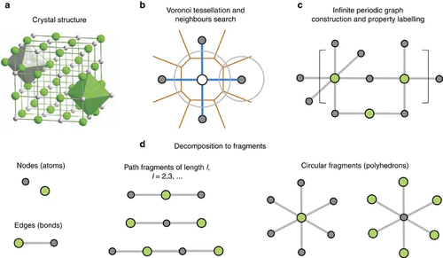
Figure 11: Schema illustrating the construction of PLMF. The concept behind this descriptor is that for crystal structure (a) the nearest neighbors are assigned using Voronoi tessellation (b) and then used to construct a crystal graph that can be colored with properties, which is then decomposed into subgraphs (d). Figure reprinted from Isayev et al.²¹⁰

A similar approach was also used in the construction of PLMF which were proposed by Isayev et al.²¹⁰ There, a crystal graph is constructed based on the nearest-neighbor assignment from the Voronoi tessellation, where the nodes represent atoms that are labeled with a variety of different (elemental) properties. Then, the graph is partitioned into sub-graphs and the descriptors are calculated using differences in properties between the graph nodes (neighboring atoms) (cf. Figure 11).

The Voronoi decomposition is also used to assign the environment in the calculation of the orbital field matrix descriptor, which is the weighted sum of the one-hot encoded vector of the electron configuration.²¹¹ One hot-encoding is a technique that is frequently used in language processing and that represents the feature vector of $n$ possibilities with zeros (feature not present) and ones (feature present). In the original work, the sum and average of the local descriptors were used as descriptors for the entire structure and also suggested to gain insight into the importance of specific electronic configurations using a decision tree analysis.

Voronoi tesselation is the dual problem of Delaunay triangulation which attempts to assign points into tetrahedrons (in three dimensions, in two dimensions into triangles, etc.) which circumspheres contain no other point in its interiors. The Delaunay tesselation found use in the analysis of zeolites, where the geometrical properties of the tetrahedrons, like the tetrahedrality or the volume, have been used to build models that can classify zeolite framework types.^{212, 213}

Overall, we will see that a common approach to generate global, fixed length, descriptors is that one calculates statistics (like the mean, standard deviation or maximum or minimum) of base descriptors, that can be based on elemental properties for each site.

4.2.2 Global Descriptors

Global Correlation Function

As already indicated, some properties are less amenable to decomposition into contributions of local environments and might be better described using the full, global correlation functions. These approaches can be seen, completely analogous to the local descriptors, as approximations to the many-body expansion, for example for the energy

$$E=\sum_{i=1}^{N}E^{(1)}(\mathbf{r}_{i})+\sum_{i<j}^{N}E^{(2)}(\mathbf{r}_{i},\mathbf{r}_{j})+\sum_{i<j<k}^{N}E^{(3)}(\mathbf{r}_{i},\mathbf{r}_{j},\mathbf{r}_{k})+\dots$$ (6)

As we discussed in the context of the symmetry functions for local environments, we can choose where we truncate this expansion (two-body pairwise distance terms, three-body angular terms …) to trade-off computational and data efficiency (more terms will need more training data) against uniqueness. Similar to the symmetry functions for local chemical environments, different projections of the information have been developed. For example, the BoB representation²¹⁴ bags different off-diagonal elements of the Coulomb matrix into bags depending on the combination of nuclear charges and has then been extended to higher-order interactions in the bond-angles machine learning (BAML) representation.¹⁸⁶ A main motivation behind this approach, which has been generalized in the many-body tensor representation (MBTR) framework,²¹⁵ is to have a more natural notion of chemical similarity than the Coulomb repulsion terms. One problem with building bags is that they are not of fixed length and hence need to be padded with zeros to make them applicable for most ML algorithms.

An alternative method to record pairwise distances, that is familiar to chemists form XRD, is the RDF, $g^{(2)}(r)$. Here, pairwise distances are recorded in a binned fashion in histograms. This representation inspired Schuett et al. to build a ML model for the density of states (DOS).²¹⁶ They use a matrix of partial RDFs, i.e., a separate RDF for each element pair—similar to how the element pairs were recorded in different bags in the BoB representation and quite similar to Valle’s crystal fingerprint²¹⁷ in which modified RDFs for each element pair are concatenated.

Von Lilienfeld et al. took inspiration in the plane-wave basis sets of electronic structure calculations, which remove many problems that local (e.g., Gaussian) basis sets can cause, e.g., Pulay forces and basis set superposition errors, and created a descriptor that is a Fourier series of atomic RDFs. Most importantly, the Fourier transform removes the translational variance of local basis sets—which is one of the main requirements for a good descriptor.¹⁷¹ The Fourier transform of the RDF also is directly related to the XRD pattern which has found widespread use in ML models for the classification of crystal symmetries.^{218, 219, 131}

For the prediction of gas adsorption properties property labeled RDFs have been introduced by Fernandez et al.²²⁰ The property labeled RDF is given by

$$\text{RDF}^{\text{P}}=f\,\sum_{i,j}P_{i}P_{j}\exp\left[-B{\left(r_{ij}-R\right)}^{2}\right],$$ (7)

where $P_{i}$ and $P_{j}$ are elemental properties of atom $i$ and $j$ in a spherical volume of radius $R$. $B$ is a smoothing factor and $f$ is scaling factor. It was designed based on the insight that for some type of adsorption processes, like CO2 adsorption, not only the geometry but also the chemistry is important. Hence, they expected that stronger emphasis on e.g. the electronegativity might help the ML model.

Structure Graphs

Encoding structures in the form of graphs, instead of using explicit distance information, has the advantage that the descriptors can also be used without any precise geometric information, i.e., a geometry optimization is usually not needed. In structure graphs, the atoms define the nodes and the bonds define the edges of the graph. The power of such descriptors was demonstrated by Kulik and co-workers in their work on transition metal complexes. They introduced the revised autocorrelation (RAC) functions²²¹ (which is a local descriptor that correlates some atomic heuristics, like the atom type, on the structure graph) and used it to predict for example metal-oxo formation energies,²²² or the success of electronic structure calculations.¹⁹ Recently, they also have been adapted for MOFs.²²³

For crystals, Xie and Grossmann built a graph-convolutional NN (GCNN) that directly learns from the crystal structure graph (cf. section 5.1.1) and could predict a variety of properties such as formation energy or mechanical properties as the bulk moduli for structures from the Materials Project.^{224, 225} This architecture also allowed them to identify chemical environments that are relevant for a particular prediction.

Distance-Matrix Based Descriptors

Another large family of descriptors is built around different encodings of the distance matrix. Intuitively, one might think that a representation such as the $z$-matrix, which is popular in quantum chemistry and is written in terms of internal coordinates, might be suitable as input for a ML model. And indeed, the $z$-matrix is translational and rotational invariant due to the use of internal coordinates—but it is not permutational invariant, i.e., the ordering matters. This was also a problem with the original formulation of the Coulomb matrix which encodes structures using the Coulomb repulsion of atomic charges (proton count $Z$) on the off-diagonal and rescaled atomic charges on the diagonal:¹⁶⁶

$$x_{ij}=\begin{cases}0.5\,Z_{i}^{2.4}&i=j\\ Z_{i}\,Z_{j}\,\phi\left(\|\mathbf{r}_{i}-\mathbf{r}_{j}\|\right)&i\neq j,\end{cases}$$ (8)

as one structure could have many different Coulomb matrices, depending on where one starts counting. The Coulomb matrix shares this problem with the older Weyl matrix,²²⁶ which is a $N\times N$ matrix composed of inner products of atomic positions, and in this way also an overcomplete set. To remedy this problem it was suggested to use sorted Coulomb matrices or the eigenvalue spectrum (but this violates the uniqueness criterion as there can be multiple Coulomb matrices with the same eigenspectrum). Also, to be applicable to periodic systems, eq. 8 needs to be modified.

To deal with electrostatic interactions in molecular simulations, one usually uses the Ewald-summation technique which splits one non-converging infinite sum into two converging ones. This trick has also been used to deal with the infinite summations which would occur if one attempted to use eq. 8 for periodic systems—the corresponding descriptor is known as the Ewald sum matrix.¹⁶⁶ The sine-Coulomb matrix is a more ad hoc solution to apply the Coulomb matrix to periodic systems. Here, the off-diagonal terms are calculated using a modified potential $\phi$ that introduces periodicity using a sine over the product of the lattice vectors and the vector between the two sites $i$ and $j$.¹⁶⁶

Point Cloud Based

In object recognition much success has been achieved by representing objects as point clouds.^{227, 228} This can also be applied to materials science, where solids can be represented as point clouds by sampling the structures with $n$ points. This point cloud can be then further processed to generate an input for a (supervised) ML algorithm. Such processing is often needed because most algorithms cannot to deal with irregular data structures, like point clouds, wherefore the data is often mapped to a grid.

Topological Data Analysis

A fruitful approach to generate features from point clouds is to use the persistence homology analysis rooted in topological data analysis (TDA).^{229, 230} Here, the underlying topological structures are extracted using a process called filtration. In a filtration one uses using a sequence of growing spaces, e.g., using balls of growing radii, to understand how the topological features change as a function of the radius. A persistence diagram records when a topological feature is created or destroyed. This is shown in Figure 12 where at some radius the first circles start to overlap, which is reflected in the end of a bar in the persistence diagram. Then, the circles form two holes (c), which is reflected with the birth of new bars that die with increasing radius, when the holes disappear (d).

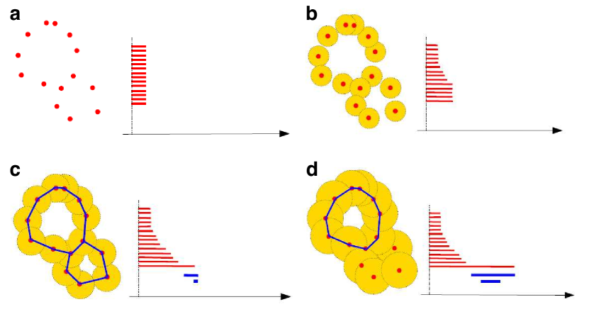
Figure 12: Illustration of the filtration of the distance function of a cloud of points. For the birth of each point, we create an interval (bar) in the persistence diagram. As we increase the radius of the points, some components die (and merge) as the circles start to overlap. The persistence diagram takes track of this by putting an end to the interval (b). As the radius of the circle further increases, we form new, one-dimensional, connected components (the holes, blue in c) and all the intervals associated with single points come to an end. The only interval that never dies is due to the union of all points. The figure is a modified version of the illustration from Chazal and Michel.²³⁰

Using this technique has recently become even easier with the scikit-tda suite of packages,²³¹ which gives an easy-to-use Python interface to the C++ Ripser library²³² and functions to plot persistent images²³³ and diagrams.

Unfortunately, most ML algorithms only accept fixed length inputs, wherefore the persistent homology barcodes cannot directly be used as descriptors. To work around this limitation, Lee and co-workers²³⁴ used a strategy that is similar to the general strategy for creating fix-length global descriptors that we discussed above, namely by computing statistics of the persistent homology barcodes (cf. section 9).
Alternative finite-dimensional representation are persistence images,²³³ which have recently employed by Krishnapriyan et al. to predict the methane uptakes in zeolites between $1\text{\,}\mathrm{bar}200\text{\,}\mathrm{bar}$ (cf. Figure 13).²³⁵

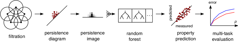
Figure 13: Illustration of the scheme used to predict gas adsorption properties using persistent images. A filtration is used to create a persistence diagram (as illustrated in Figure 12). This is then transformed into a persistence image that is used to train a RF model to predict the methane uptake. Figure redrawn based on ref. ²³⁵

In persistence images, the birth-death pairs $(b,d)$, which are shown in persistence diagrams, are transformed into birth-persistence pairs $(b,d-b)$ which are spread using a Gaussian. The images are then created by binning the function of $(b,d-b)$. Krishnapriyan et al. then used RFs to learn from this descriptor, but it might also be promising to investigate the use of transformations of the homology information that can be learned during training (e.g., using NNs, see section 5.1.1).²³⁶

The capabilities of TDA have been demonstrated in the high-throughput screening of the nanoporous materials genome.^{237, 238} Here, the zeo++ code has been used to analyze the pore structure of zeolites (using Voronoi tessellations), which then could be sampled to create point clouds that were used as an input for a persistent homology analysis, which output was summarized in persistence diagrams (“barcodes”). The similarity between these persistence diagrams was then used to rank the materials, i.e., if the persistence diagram of one structure is similar to a high-performing structure, it is likely to also perform well. As Moosavi, Xu et al. recently showed, the similarity between barcodes can also be used to build kernels for KRR which then can be used to predict the performance for methane storage applications.¹⁸⁵

Neural-Network Engineered Features

A promising alternative to TDA is to use specific NN architectures such as PointNet that can directly learn from point cloud inputs.²²⁸ DeFever et al. used the PointNet for a task similar to object recognition: the classification of local structures in trajectories of molecular simulations.²³⁹ Interestingly, the authors also demonstrated that one can use PointNet to create hydrophilicity maps, e.g., for self-assembled monolayers and proteins.

Coarse Tabular Descriptors

Our discussion so far guided us from atomic-level descriptors to more coarse, global descriptors. In this section, we will explore some more examples of such coarse descriptors. Those coarse descriptors are frequently used in top-down modeling approaches, where a model is trained on experimental or high-level properties. Obviously, such coarse, high-level descriptors are not suited to describe properties with atomic resolution, e.g., to describe a PES, but they can be efficient to model, for example, gas adsorption phenomena.

Based on Elemental Properties

Widely used in this context are compositional descriptors that encode information about the chemical elements a compound is made up of. Typically, one finds that simple statistics such as sums, differences, minimums, maximums or covariance of elemental properties such as electronegativity or covalent radii are calculated and used as feature vectors. There has been some success with using such descriptors for perovskites^{240, 241}, half-Heussler compounds²⁴², analysis of topological transitions,²⁴³ the likelihood of substitutions^{244, 245} as well as the conductivity of MOFs.²⁴⁶ Generally, one can expect such descriptors to work if the target property is directly related to the constituent elements. A prime example of this concept are perovskites for which there are empirical rules, like the Goldschmidt tolerance factor, that relate the radii of the ions to the stability, wherefore it is reasonable to expect that one can build meaningful ML models for perovskite stability, that outperform the empirical rules, with ion radii as features.

Cheap Calculations Crude Estimates of Target and Experimental Features

Especially for our case-study problem, the gas adsorption in porous materials, tabular descriptors that are based on cheap calculations (e.g., geometry analysis, energy grids) are most commonly used. As gas adsorption requires that the pore properties are “just right” it is natural to calculate them and use them as features.^{247, 248, 249, 250} Especially, since we know that target similarity governs the error of ML models.¹⁸⁶ Typically, such descriptors, as the pore size distribution (PSD),²⁵¹, and accessible surface areas or pore volumes, can be computed with programs as Zeo++,²⁵² Poreblazer²⁵³ or MOFomics/ZEOMICS.^{183, 182}

A cheaper calculation was also used by Bucior et al. to construct descriptors. On a coarse grid they computed the interactions between the adsorbate and the framework, summarized this data in histograms and then used these histograms to construct ML models for the adsorption of H2.²⁵⁴ This is the related to the approach Zhang and Ling put forward to use ML on small datasets.²⁵⁵ They suggest including crude estimates of the target property into the feature set. As an example, they included force-field derived bulk moduli to predict bulk moduli on DFT level of theory. This idea is directly related to $\Delta$-ML and co-kriging approaches which we will discuss below in more detail.

Especially when one uses a large collection of tabular features it can be useful to curate feature dictionaries, which describe what the feature means and why it is useful—to aid collaboration and model development.

Using Building Blocks as Features

For materials like MOF, COF, or also polymers that are constructed by self-assembly of simpler building blocks, one can attempt to directly use the building blocks as features. Here, one typically one-hot encodes the presence of building blocks with ones and the absence with zeros. Therefore, there will be as many columns in the feature matrix as there are building blocks. Due to the nature of this encoding, such a model cannot generalize to new building blocks. This featurization was for example used by Borboudakis et al. who one-hot encoded linker and metal node types to learn gas adsorption properties of MOFs from a small database.¹⁷² Recently, Fanourgakis et al. reported a more general approach in which they use statistics over atom types (e.g., minimum, maximum and average of triple bonded carbon per unit cell), that would usually be used to set up force field topologies, as descriptors for RF models to predict the methane adsorption in MOFs.²⁵⁶

4.3 Feature Learning

4.3.1 Feature Engineering

A key insight is that the “raw” features are often not the best inputs for a ML model. Therefore, it can be useful to transform the features. This is also what every chemist or modeler already intuitively knows: Some phenomena like the dependence of the activation energy on the diffusion constant are better visible after a logarithmic transformation. Sometimes it is also more meaningful to look at ratios, like the Goldschmidt tolerance ratio, rather than at the raw values.

The term feature engineering describes this process where new features are formed via the combination and/or mathematical transformation of raw features. And this is one of the main avenues for domain knowledge to enter into the modeling process. One approach to automate this process is to automatically try different mathematical operations and transformation functions as well as combinations of features. Unfortunately, this leads to an exponential growth of the number of features and the modeler now faces the problem to select the best features to avoid the curse of dimensionality (cf. section 4.1), which is not a trivial problem. In fact, the featurization process is equivalent to finding the optimal basis set for the description of a physical problem.

4.3.2 Feature Selection

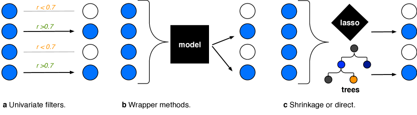
Figure 14: Overview of different feature selection strategies. Figure redrawn based on an illustration by Janet et al.²²¹

For some phenomena one would like to develop ML models but it might not be a priori clear which descriptors one should use to describe the phenomenon, e.g., because it is a complex multi-scale problem. Intuitively, one might try all possible combinations of descriptors that one can come up with to find the smallest, most informative set of features to avoid the curse of dimensionality. But this approach is deemed to fail as it is a non-deterministic polynomial-time (NP) hard problem. This means that a candidate solution for this problem can be verified in polynomial time, but that the solution itself can probably not be found in polynomial time. Hence, approximations or heuristics are needed to allow us to make the problem computationally tractable. One generally distinguishes three approaches to tackle this problem: First, simple filters can be used to filter out features (e.g., based on correlation with the target). Second, iterations in wrapper methods (pruning, recursive feature elimination) can be used to find a good subset, or one can attempt to directly include the objective of minimizing the dimensionality in the loss function.^{257, 258, 221, 259}

Filter Heuristics

Given a large set of possible features one can use some heuristics to compact the feature set. A simple filter is to use the correlation, mutual information²⁶⁰ or fitting errors for single features as surrogates and only use the features that show the highest correlation or mutual information with the target or the ones for which a simple model shows the lowest error. Obviously, this approach is unable to capture interaction effects between variables.

Another heuristic that can be used to eliminate features is to eliminate those that do not show a lot of variance (VarianceThreshold in sklearn). The intuition here is that (nearly) constant features cannot help the model to distinguish between labels.

This is to some extent similar to PCA based feature engineering, where one tries to find the linear combinations of features that describe most of the variance and then only keeps those principal components. This approach has the drawback that arbitrary linear combinations are not necessarily physically meaningful and that explaining the variance does not necessarily mean being predictive.

Wrapper Approaches

Often, one also finds stage-wise feature selection approaches.²⁶¹ Either by weight pruning, i.e., by fitting the model on all features and then removing those with low weights or by recursive feature elimination (RFE). RFE starts by fitting a model on all features and then iteratively removes the least important features until a desired number of features is reached. This iterative procedure is needed because the feature importance can change after each elimination, but it is computationally expensive for moderately sized feature sets. The opposite approach, i.e., the iterative addition of features is known as recursive feature addition (RFA) and is often used in conjunction with RF feature importance, which is used to decide which features should be included. This approach was for example used in a work by Kulik and co-workers in which they built models to predict metal-oxo formation energies, which are relevant for catalysis. In doing so, they found that they can reduce the size feature set from ca. 150 to 22 features using RF-RFA which led to reduction of the mean absolute error (MAE) on the test set from $9.5\text{\,}\mathrm{k}\mathrm{c}\mathrm{a}\mathrm{l}\mathrm{/}\mathrm{mol}$ to $5.5\text{\,}\mathrm{k}\mathrm{c}\mathrm{a}\mathrm{l}\mathrm{/}\mathrm{mol}$.²²²

Direct Approximations: LASSO/Compressed Sensing

As an alternative to iterative approaches, there are efforts to use objective functions that directly describe both modeling goals: First, to find a model that minimizes the error and, second, to find a model that minimizes the number of variables (following Occam’s razor, cf. section 4.1). In theory, this can be achieved by adding a regularization term $\|\mathbf{w}\|^{p}=\left(\sum_{i=1}^{n}w_{i}^{p}\right)^{1/p}$ to the loss function and attempting to find the coefficients $\mathbf{w}$ that minimize this loss function. In the limit $p=0$, there is nothing won as it is the NP hard problem of minimizing the number of variables, we mentioned above.²⁶² Hence, the $l_{1}$ norm (also known as Taxicab or Manhattan norm), i.e., the case $p=1$, is often used as an approximation (to relax the $l_{0}$ condition).²⁶³ This has the advantage that the optimization is now convex and that the edges of the regularization region tend to favor sparsity (cf. Figure 30 and accompanying discussion for more details). The minimization of the $l_{1}$ known is known in statistics as the least absolute shrinkage and selection operator (Lasso) and widely used to avoid overfitting (regularization), by penalizing high weights (cf. section 6.2.1).²⁶³ Compressed sensing²⁶⁴ uses this idea to recover a signal with only a few sensors while giving conditions on the design matrix (with materials in the rows and the descriptors in the columns) for which the $l_{0}$ and the Lasso solution will likely coincide. An in-depth discussion of the formalism of feature learning using compressed sensing is given by Ghiringhelli et al.²⁶² This approach works well in materials science as many physical problems are sparse and it also works well with noise, which is also common to physical problems.²⁶⁴ Ghiringhelli et al. applied this idea to materials science but also highlighted that a procedure based only on the Lasso has difficulties in selecting between correlated features and dealing with large feature spaces.¹⁶⁵ With sure independence screening and sparsifying operator (SISSO) Ouyang et al. add a sure independence (si) layer before the Lasso.²⁶⁵ This si layer pre-selects a subspace of features that show the highest correlation with the target and that can then be further compressed using the Lasso. This approach, for which open-source code was published,²⁶⁶ allowed Scheffler and co-workers to construct massive sets of ${10}^{9}$ descriptors using combinations of algebraic functions applied primary features, like the atomic radii, and to discover new tolerance factors for the stability of perovskites²⁴¹ or to predict new quantum spin-Hall insulators using interpretable descriptors.²⁴³

Another approach to the feature selection problem uses projected gradient descent to locally approximate the minimization of the $l_{0}$ norm.²⁶⁷ It is efficient as it uses the gradient and it achieves sparsity by, stepwise, setting the smallest components of the weights vector $\mathbf{w}$ to be zero (cf. Listing 2 for pseudocode).^{268, 269}

Listing 2: Pseudo-code for iterative hard thresholding (also known as projected gradient descent).

⬇

1i = 0

2weights_i = intitialize_weights()

3k = 5 # hyperparameter that needs to be tuned

4

5while halting condition not fulfilled:

6 # select a stepsize for gradient descent

7 eta[i] = chose_stepsize()

8 # perform the gradient descent step

9 chi[i] = weights_i - eta[i] * gradient(lossfunction(weights[i]))

10 # select the largest component

11 weights[i+1] = select_k_large_components(chi[i], k)

12 # update the counter

13 i = i + 1

A modified version was also used Pankajakshan et al.^{270, 271} They combined this feature selection method with clustering (to combine correlated features) and created a representative feature for each cluster, which they then used in the projected gradient algorithm to compress the feature set. Additionally, they also employed the bootstrap technique to make their selection more stable.

The bootstrapping step is also the key to another method known as stability selection. Here, the selection algorithm (e.g., the Lasso) is run on different bootstrapped samples of the dataset and only those features that are important in every bootstrap are selected, which can help to counter chance correlation.²⁷² This is currently being implemented as randomized Lasso in the sklearn Python framework.

4.3.3 Data Transformations

An additional problem with features is that their distribution or the scale on which they are on (e.g., due to the choice of units) might not be appropriate for ML. One of the most important reasons to transform data is to improve interpretability. Some features are more natural to think about on a logarithmic scale (e.g., the concentration of protons is known as $\text{pH}=-\lg_{10}\ce{H3O^{+}}$ in chemistry and also the Henry coefficient is naturally represented on logarithmic scale), or reciprocal scale (e.g., temperature in the case of Arrhenius activation energy analysis). In other cases, the underlying algorithm will profit from transformations, e.g., if it assumes a particular distribution for the data (e.g., the archetypal linear regression assumes a normal distribution of the residuals). The most widely used transformations are power transformations like the Box-Cox (defined as $(x^{\lambda}-1)/\lambda$ for $\lambda>0$, $\ln x$ for $\lambda=0$, where $\lambda$ can be used to tune the skew),²⁷³ the inverse hyperbolic sine^{274, 275} or the Yeo-Johnson transformation which all aim to make the data more normally distributed. The Box-Cox transformation, or a simple logarithmic transformation ($\lg x$), are the most popular techniques, but the inverse hyperbolic sine and the Yeo-Johnson transformation have the advantage that they can also be used on negative values.

Normalization and Standardization

In the following, we will show that many algorithms perform interference by calculating distances between examples. But in the physical world, our features might have different scales, e.g., due to the arbitrary choice of units. Surface areas might be recorded as numbers in the order of ${10}^{3}$ and void fractions as numbers on the order of ${10}^{-3}$. For ML one wants to remove such influences from the model, as illustrated in Figure 15.

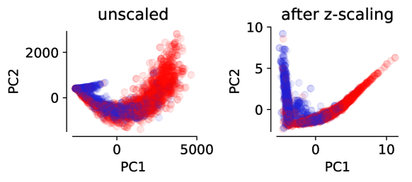
Figure 15: Influence of scaling, here standard scaling (z-scaling), of features on the dimensionality reduction using PCA. For this example we used the data from Boyd et al. and performed the PCA on the feature matrix of pore properties descriptors and plot the data in terms of the first two principal components (PC1, and PC2). We then color code the structures with above-median CO2 uptake (red) different from those with below-median CO2 uptake (blue) and plot the points in random order. It is observable that the separation after scaling is clearer.

Also, optimization algorithms will have problems if different directions in feature space have different scales. This is intuitive if we look at the gradient descent update step, where the values of the features, $x_{i}$, are directly involved and for which reason some weights might update faster than others (using a fixed learning rate $\eta$).

The most popular choices to remedy these problems are min-max scaling and standard scaling ($z$-score normalization). Min-max scaling transforms features to a range between zero and one (by subtracting the minimum and dividing by the range), and in this way minimizes the effect of outliers. In contrast to that, the standard scaling transforms feature distributions to distributions centered around zero and unity variance by subtracting the mean and diving by the standard deviation. Note that by using this transformation we do not bind the range of features, which can be important for some analyses like PCA, which work on the variance of the data.

In case there are many outliers or strong skew, it might be more reasonable to scale data based on robust estimators of centrality and spread, like subtracting the median and dividing by the interquartile range (this is implemented as RobustScaler in sklearn).

It is important that those transformations need to be applied to training and test data—but using the distribution parameters “learned” from the training set. If we computed those parameters also on the test set we would risk data leakage, i.e., provide information about the test data to the model.

Decorrelation

Often, one finds oneself in a position where the initial feature set contains multiple variables that are highly correlated with each other, like gravimetric and volumetric pore volumes or surface areas. Usually, it is better to remove those correlations. The reasoning behind this is that multicolinearity usually means that there is data redundancy, which violates the minimum description length principle we discussed above (cf. section 4.1). In particular severe cases, it can make the predictions unstable (and also the feature selection as we discussed above) and in general it undermines causal interference as it is not clear which of the correlated variables is the reason for a particular prediction.^{276, 277}

Widespread ways to estimate the severity of multicolinearity is to use pair-correlation matrices or the variance inflation factor (VIF), which estimates how much of the variance is inflated by colinearity with other features.^{278, 279} It does this by predicting all the features using the remaining features $\text{VIF}=1/(1-R_{i}^{2})$, where $R_{i}$ is the coefficient of determination for the prediction of feature $i$. A VIF of ten would mean that the variance is ten times larger than it would be for fully orthogonal features.

5 How To Learn: Choosing a Learning Algorithm

After data selection (cf. section 3 and featurization (cf. section 4) one can proceed to training a ML model. But also here, there are a lot of choices one can make. In Figure 16 we give a non-exhaustive overview of the learning algorithm landscape.

In the following, we discuss some rules of thumb that can help to choose the appropriate algorithm for a given problem and discuss the principles of the most popular ones. Typically, we will not distinguish between classification and regression as many algorithms can be formulated both for regression and classification problems.

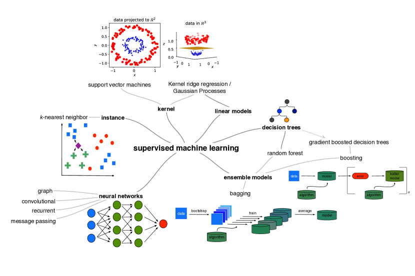
Figure 16: Overview of the supervised ML algorithm landscape. We do not distinguish between classification and regression as many of the algorithms can be formulated both for regression and classification problems.

Principles of Learning

One of the main principles of statistical learning theory is the bias-variance decomposition (cf. eq. 9), which describes that the total error can be described as the sum of squared bias, variance and an irreducible error (Bayes error)

$$\text{error}=\text{bias}^{2}+\text{variance}+\text{Bayes error},$$ (9)

and can easily be derived by rewriting of the cost function for the mean square error.⁷ The variance of a model describes the error due to finite training size effects, i.e., how much the estimation fluctuates due to the fact that we need to use a finite number of data points for training and testing (cf. Figure 17). The bias is the difference between the prediction and the expectation value; it is the error we would obtain for an infinite number of training points (cf. Figure 17). In this case, the bias represents the limit of expressivity for our model, e.g., that the order of the polynomial is not high enough to describe the problem that should be modeled. But this error could in principle be removed by choosing a better model. All the remaining error, which cannot be removed by building a better model, is for example due to noise in the training data. For this reason, this term is called irreducible error (also known as Bayes error).

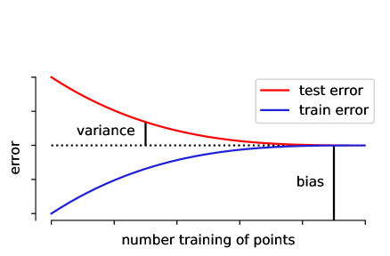
Figure 17: Train and test error as a function of the number of training points and the definition of bias and variance; bias being the error that remains on the training set for an infinite number of training points, and variance the error due to the finite size of the training set.

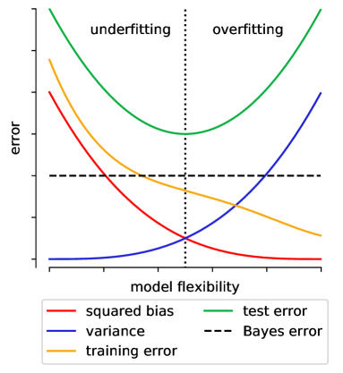
Figure 18: Bias, variance, training, and test error as well as Bayes error (irreducible error) as function of the model flexibility.

This trade-off between bias and variance is directly linked to model flexibility. A highly flexible model, which is also often less interpretable, like a high-order polynomial, tends to have a high variance whereas a simple model, such as a regularized linear regression, tends to have a high bias (cf. Figure 18). In practice, it is often useful to first create a model that overfits, hence has close to zero training error, and in this way ensure that the expressivity is high enough to model the phenomenon. Then, one can use techniques which we will describe in section 6 to reduce overfitting.²⁸⁰

The classical bias variance-trade-off curve (cf. Figure 18) suggests that there is a “sweetspot” (dotted line) in which the test error is minimal. One current research question in deep learning (DL) is why one still can achieve good testing error with highly overparameterized models, i.e., models for which the number of parameters is larger than the number of training points.^{281, 282} Belkin et al. suggest that “modern”, overparameterized, models do not work in the regime described by the bias-variance trade off curve in Figure 18. Rather, they suggest a double descent curve where following a jamming transition, when we reach approximately zero train error (the interpolation threshold), the error decreases with the number of parameters.²⁸³ Belkin et al. hypothesize that this is due to the larger function space that is accessible to more complex models which might allow them to find interpolating functions that are simpler (and hence better approximations according to Occam’s razor, cf. section 4.1).

In the following, we give an overview of the most popular learning techniques. We see NNs mostly suited for large, unstructured, datasets, data sources, e.g.  images or spectra, or feature sets which are not yet highly preprocessed (e.g., directly using the coordinates and atom identities)—as NNs can also be used to create features (representation learning), which in the chemical science is often used in a “message passing” approach (cf. section 5.1.1).²⁸⁴

5.1 Lots of (Unstructured) Data (Tall Data)

In (computational) materials science a large array of data is created every day and some of it is even deposited in a curated form on repositories. Still, most of it does not contain highly engineered features. To learn from such large amounts of data NN are one of the most promising approaches. The field of DL, which describes the use of deep NNs, is too wide to be comprehensively reviewed, wherefore we just give an overview of the basic building principles of the most popular building blocks.

5.1.1 Neural Networks

Classical, feed-forward, NN approximate a function $f$ using a chain of matrix evaluations

$$f(\mathbf{X})=g^{(L)}\left(\mathbf{W}^{(L)}\cdots g^{(2)}\left(\mathbf{W}^{(2)}g^{(1)}\left(\mathbf{W}^{(1)}\mathbf{X}\right)\right)\right),$$ (10)

where $\mathbf{X}$ is the input vector, $g$ are activation functions—non-linear functions such as sigmoid functions or the rectified linear unit (ReLU)—and the $\mathbf{W}$ are the weight matrices the neural network learns using the data. $L$ is here the number of layers, and the most popular and promising case is when there are multiple nonlinear layers. This is known as DL. The multiplication with the weight matrix is a linear transformation of the data, the bias corresponds to a translation and the activation function enables us to introduce non-linearities.

One of the most frequently cited theorems in the DL community is the universal approximator theorem which states that, under given constraints, a single hidden layer of finite width is able to approximate any continuous function (on a set of $\mathbb{R}$). What is perhaps more surprising is that those models work, that we can train them on random labels without any convergence problems,²⁸⁵ and that they still generalize—these questions are active areas of research in computer science.

One of the strengths of neural networks is that they scale really well since training them does not involve an expensive matrix inversion (which scales with $\mathcal{O}(n^{3})$) and since they can be trained efficiently in batch mode with stochastic gradient descent, where only a small part of the complete data needs to be loaded into memory. The large expressivity of deep networks combined with the benign scaling makes them the preferred choice for massive (unstructured) datasets, whereas classical statistical learning methods might be the preferred choice for small datasets of structured data.²⁸⁶

High-Dimensional Neural Network Potential

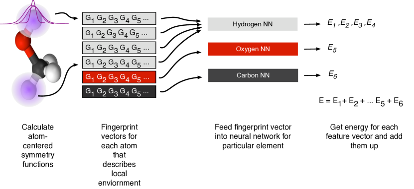
Figure 19: Schematic representation of the architecture of a HDNNP (Behler-Parinello scheme) at the example of methanol. The local environment around each atom is described with symmetry functions (pink, Gaussians). Each symmetry function can probe different length scales and will return one value. The values can then be concatenated into one fingerprint vector. This fingerprint vector can then be fed into a NN corresponding to one particular element, i.e., we will feed the four fingerprints for the four hydrogens into the same neural network but will receive different outputs due to the different fingerprints. The predictions can then be added up to calculate the energy of the entire system.

One of the cases where neural networks shine in the field of chemistry are high-dimensional neural networks that can be used to “machine learn” potential energy surfaces—as it has recently been done for MOF-5 (cf. section 9),²⁸⁷ and which can be used to access time or length scales that are not accessible with ab initio techniques at accuracies that are not accessible with force fields. One prime example is the ANI-1X potential, which is a general-purpose potential that approaches coupled-cluster theory accuracy on benchmark sets.^{118, 288} And due to the nature of molecular simulation in which there is a lot of correlations between the properties at different time steps, and hence data redundancy, they are an ideal application for ML.²⁸⁹

NN models for potential energy surface have already been proposed more than two decades ago. But due to the architecture of those models, it was difficult to scale them to larger systems and the models did not incorporate fundamental invariances of the potential.²⁹⁰ This has been overcome with the so-called HDNNP (also known as Behler-Parinello scheme, cf. Figure 19). Each atom of the structure will be represented by a fingerprint vector (using symmetry functions) that describes its chemical environment within a cutoff radius (cf. chemical locality approximation in section 4.1). For each element, a separate NN is trained (cf. Figure 19) and each atomic fingerprint vector is fed into its corresponding NN that predicts an energy. The total energy is then the sum of all atomic contributions (cf. eq. 1). This additive approach is scalable by construction (nearly linear with system size) and the invariances with respect to rotation and translation are introduced on the level of the symmetry functions. Also, the weight sharing (one NN for many environments of a particular element) makes this approach efficient and allows for generalization (similar to the sharing of filters in CNN which we will discuss in section 5.1.1). One additional advantage of such models is that they are not only efficient and accurate, but that they are also reactive (again due to the locality assumption combined with the fact that no functional form is assumed)—which most classical force fields are not. For more technical details, we recommend reviews from Behler.^{291, 124}

Message-Passing Neural Networks/Representation Learning

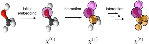
Figure 20: Schematic illustration of the idea behind the message-passing architecture. Following the initial embedding of the molecule each environment $\chi$ represents one atom. Successive interactions in the message passing architecture refine the local chemical environments $\chi$ by taking into consideration the interaction between the neighboring environments.

In message-passing neural networks, the input can be nuclear charges and positions, which are also the variables of the Schrödinger equation. A DNN then constructs descriptors that are relevant for the problem at hand (representation learning). The idea behind this approach is to build descriptors $\chi$ by recursively adding interactions $v$ with more and more complex neighboring environments at a distance $d_{ij}$ (cf. Figure 20)

$$\chi_{i}^{(t+1)}=\chi_{i}^{(t)}+\sum_{j<i}\mathbf{v}\left(\chi_{j}^{(t)},d_{ij}\right).$$ (11)

This approach is for example used in deep tensor neural network (DTNN),²⁹² SchNet,²⁹³, SchNOrb,²⁹⁴ hierarchically interacting particle (HIP)-NN,²⁹⁵ and PhysNet.²⁹⁶ A detailed discussion of this architecture type is provided by Gilmer et al.²⁸⁴

Images or Spectra

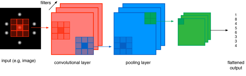
Figure 21: Example of the use of a CNN. One slides convolution layers (red) over an image, which for example can be a two-dimensional diffraction pattern.¹³¹ Usually, one then uses a pooling layer to compress the matrices after convolution. After flattening, the output can be used for conventional hidden NN layers.

For learning from images or patterns, CNN are particularly powerful. They are inspired by the concept of receptive fields in biological processes, where each neuron responds only to activation in a specific region of the visual field.

CNNs work by sliding a filter matrix over the input to extract higher-level features (cf. Figure 21). An example of how such filters work is the set of the Sobel filter matrices, which can be used as edge detectors:

$$\mathbf{G}_{x}=\begin{pmatrix}1&0&-1\\ 2&0&-2\\ 1&0&-1\end{pmatrix}.$$ (12)

The middle column, which is centered on the cell (pixel) on which the filter is used, is filled with zeros and the column left and right to it have opposite signs. In case there is no edge, the values on the left and the right of the pixel will be equal. But in case there is an edge, this is no longer the case and the matrix multiplication will give a result that highlights the edge. By sliding the $\mathbf{G}_{x}$ matrix horizontally over an image one can hence highlight horizontal edges. A collection of different filter layers are used to learn the different correlations between (neighboring) elements. CNN apply, on each layer, a set of different filters that share weights (similar to the way in which different atoms of the same element share weights in HDNNP). Usually, convolutions are used together with pooling layers that compress the matrix by, again, sliding a filter matrix, which for example takes the maximum or the average in a $2\times 2$ block of the matrix, over the matrix (cf. Figure 21). This leads to approximate translational invariance as the maximum pixel after the convolution will still be extracted by a maximum pooling layer if the translation was not too large (since the pooling effectively filters out small translations).

CNNs tend to generalize well and are computationally efficient due to the weight sharing between the different filter layers for each convolutional layer. Not surprisingly, ample works attempted to use CNNs to analyze spectra. Ziletti et al. used this approach to classify crystal structures based on two-dimensional diffraction patterns.¹³¹ Others used them to perform classification based on steel microstructures,¹³⁰ or a representation based on the periodic table, where the positions of the elements of full-Heussler compounds were encoded and the authors hoped to implicitly leverage the information encoded in the structure in the periodic table using the CNN.²⁹⁷

Case Study: Predicting the Methane Uptake in COFs Using a Dilated CNN

For this case study, we use the XRD pattern as a geometric fingerprint of the structure as it fulfills many of the criteria for an ideal descriptor: it is cheap and invariant to symmetry operations like an expansion of the unit cell. But the way in which information is encoded in the fingerprint makes it not suitable for all learners: one could try using it in kernel machines to do similarity-based reasoning—similar to what von Lilienfeld and co-workers have done with radial distribution functions.¹⁷¹ However, one could also try to create a “pattern recognition” model—this is where CNNs are powerful. Importantly, the patterns do not only span a small range, like neighboring reflexes, but are composed of both nearby and far-apart reflexes (due to the symmetry selection rules). For this reason, conventional convolution layers might be not ideal. We use dilated convolutions to exponentially increase the receptive field: Dilated convolutions are basically convolutions with holes and in our model for which we increase the hole size from layer to layer. To avoid overfitting, we use spatial dropout, which is especially well suited for convolutional layers (cf. section 5.1.1) and which randomly deactivates some neurons.

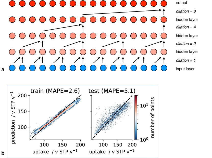
Figure 22: Using a dilated CNN to predict the methane uptake of COFs assembled by Mercado et al.²⁹⁸ For this example, we use dilated convolutions to extract correlations from the XRPD pattern (a). We can then pass the output to some hidden layers to predict the methane uptake (b). We overfit to the training set, but can also get decent performance on the test set without major tuning of the model. MAPE is an acronym for the mean absolute percentage error.

From Figure 22 we see that such a model is indeed able to predict the deliverable capacity for methane in COFs based on the XRD pattern.

Sequences

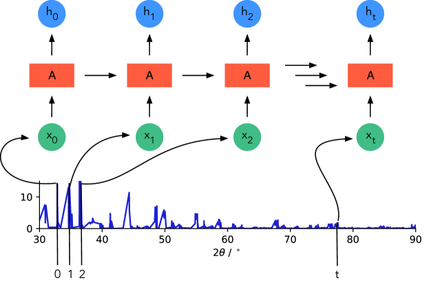
Figure 23: Schematic illustration of the building principle of a RNN. A NN $A$, uses some input $x$, like a peak of a XRPD pattern, to produce some output $h$. Importantly, some information is passed from one NN to the next.

RNNs are frequently used for the modeling of time-series data as they, in contrast to classical feed-forward models, have a feedback loop that gives the network a “memory” which it can use to recognize information that is encoded in the sequence itself (cf. Figure 23). This fitness for temporal data was for example used by van Nieuwenburg to classify phases of matter based on their dynamics, which in their case was a sequence of magnetizations.²⁹⁹ Similarly, Pfeiffenberger and Bates used a RNN to find improved protein conformations in molecular dynamics (MD) trajectories for protein structure prediction.³⁰⁰

Another approach to model sequences is to use autoregressive models, which also incorporate reference to $p$ prior sequence points

$$X_{t}-\phi_{1}X_{t-1}-\phi_{2}X_{t-2}-\cdots-\phi_{p}X_{t-p}=\epsilon_{t},$$ (13)

where $\phi_{p}$ are the parameters of the model and $\epsilon$ is white noise. This approach has for example been used by Long et al. to model the degradation of lithium-ion batteries based on their capacity as a function of the number of charge/discharge cycles.³⁰¹

Graphs

As indicated above (cf. section 4.2.2), graphs are promising descriptors of molecules and crystals as they can provide rich information without the need for precise geometries. But learning from the graph directly requires special approaches.

Figure 24: Schematic illustration of the crystal graph CNN developed by Xie and Grossman.²²⁴ Reprinted from Xie and Grossman,²²⁴ Copyright (2018) by the American Physical Society. After representing the crystal structure as a graph (a) by using the atoms as nodes and the bonds as edges, the graph can be fed into a graph CNN (b). For each node of the graph, $K$ convolutional layers and $L_{1}$ hidden layers are used to create a new graph that is then, after pooling, send to $L_{2}$ hidden layers.

Similar to message passing neural networks, Xie and Grossman developed convolution operations on the structure graph that let an edge interact iteratively with its neighbors to update the descriptor vector (cf. Figure 24) and in this sense is a special case of the message-passing NNs (cf. section 5.1.1).²²⁴ Again, this approach has been shown to be promising in the molecular domain before it has been applied to crystals.³⁰²

5.2 Limited Amount of (Structured) Data (Wide Data)

Especially for structured data, conventional ML models, like kernel-based models, can often perform equally or better than neural networks—especially when the amount of data is limited. In any case, it is generally useful to implement the simplest model possible first, to have a baseline and also to ensure that the infrastructure (getting the data into the model, calculating metrics …) works before starting to implement a more complex architecture.

5.2.1 Linear and Logistic Regression

The most widely known regression method is probably linear regression. In its ordinary form, it assumes a normal distribution of residuals, but we want to note that also generalized versions are available that work for other distributions. One significant advantage of linear regression is that it is simple and interpretable. One can directly inspect the weights of the model to understand how predictions are made and it has been the workhorse of cheminformatics. Even though the simple architecture limits the expressivity of the model this is also a feat as one can use it for initial debugging, feedback loops, and to get some initial baseline results.

5.2.2 Kernel Methods

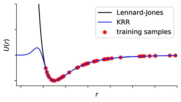
Figure 25: KRR to learn the Lennard-Jones (12,6) potential. We randomly sampled 80 points on the potential, then tuned the hyperparameters of the kernel and then predicted for all points. The model fails completely to model the strong repulsion due to the lack of training examples in that region.

One of the most popular learning techniques in chemistry is KRR. The core idea behind kernel methods is to improve beyond linear methods by implicitly mapping into a higher-dimensional space which allows treating non-linearities in a systematic and efficient way (cf. Figure 26).

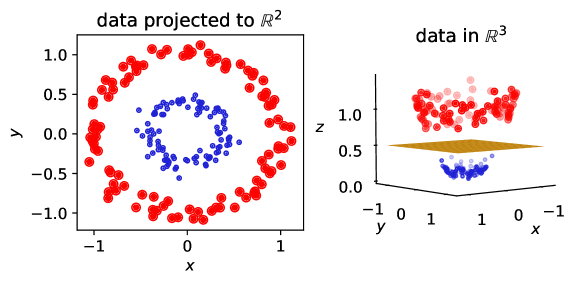
Figure 26: Visualization of one idea behind the kernel trick—mapping to higher-dimensional spaces to make problems linearly separable. In two dimension, the data (two different classes, colored in red and blue, respectively) is not linearly separable, but after applying the kernel $K(x,y)=x\cdot y+\|x\|^{2}=\|y\|^{2}$ we can draw a plane to separate the classes (three-dimensional plot on the right).

A naive approach for introducing non-linearities would be to compute all monomials of the feature columns, e.g., $\phi(x_{1},x_{2})=(x_{1}^{2},x_{1}x_{2},x_{2}x_{1},x_{2}^{2})$. But this can become computationally infeasible for many features. The kernel trick avoids this by using kernel functions, i.e., inner products in some feature space.³⁰³ If they are used, the computation scales no longer with the number of features but with the number of data points.

There are strict mathematical rules that govern what a function needs to fulfill to be a valid kernel (Mercer’s theorem),³⁰³ but the most popular choices for kernel functions are the Gaussian ($K(x,x^{*})=\exp\left(\gamma\|x-x^{*}\|^{2}\right)$) or the Laplacian ($K(x,x^{*})=\exp\left(\gamma\|x-x^{*}\|\right)$)) kernels, which width ($\gamma$) controls how local the similarity measure is.

The general intuition behind a kernel is to not consider the isolated data points but rather the similarity between a query point $x$, for which we want to make a prediction, and the training points $x^{*}$ (landmarks, which are usually multi-dimensional vectors), and to measure this similarity with inner products (as many algorithms can be rewritten in terms of dot products). At the same time, one then uses this similarity measure to work implicitly in a higher-dimensional space where the data might be easier separable. That is, it is most useful to think about predictions with KRR using the following equation

$$\underbrace{y(x)}_{\text{prediction}}=\sum_{i}\underbrace{a_{i}}_{\text{weight}}\,\overbrace{K(\underbrace{x_{i}^{*}}_{\text{landmark}},\underbrace{x}_{\text{query point}})}^{\text{kernel}},$$ (14)

or in matrix form, we write

$$\mathbf{y}=\mathbf{K}\,\mathbf{a}\quad\Leftrightarrow\quad\mathbf{a}=\mathbf{K}^{-1}\,\mathbf{y}.$$ (15)

But this equation assumes that $\mathbf{K}^{-1}$ can be found, which might not be the case if there is no $\mathbf{K}$ or more than one $\mathbf{K}$ that satisfies the equation (i.e., it is an ill-posed, unstable or non-unique, problem). For this reason, one typically adds a regularization term $\lambda\mathbf{I}$, with $\mathbf{I}$ being the identity matrix (we will explore the concept of regularization in more depth and from another viewpoint in section 6) which acts as a high-pass filter, i.e., it filters out the noise and makes the inversion more stable and the solution smoother. One then solves

$$\mathbf{a}={\left(\mathbf{K}+\lambda\mathbf{I}\right)}^{-1}\,\mathbf{y}.$$ (16)

The most widely known algorithms which use this kernel trick are support vector machines (SVMs) and KRR. They are equivalent except for the loss function and the fact that the KRR is usually solved analytically. The SVMs use a special loss function, the $\epsilon$-insensitive loss, where errors smaller than $\epsilon$ are not considered. The KRR, on the other hand, uses the ridge loss function, which penalizes high weights and which we will discuss in section 6.2.1 in more detail.

One virtue of kernel learning is the mathematical framework which it provides. It allows deriving a scheme in which data of different fidelity can be combined to predict on the high-fidelity level—a concept that was used to learn using a lot of general-gradient approximation (GGA) data (PBE functional) to predict hybrid functional level (HSE06 functional) band gaps.³⁰⁴ We will explore this concept, that can be promising for the ML of electronic properties of porous materials with large unit cells, in more detail in section 10.3.

Also, kernels pave an intuitive way to multitask predictions; by using the same kernel for different regression tasks and predicting the coefficients for the different tasks at the same time, Ramakrishnan and von Lilienfeld could predict many properties from only one kernel (computing the Kernel is usually the expensive step as it involves a matrix inversion which scales cubically).³⁰⁵ Due to the relative ease of use of kernel methods and their mathematical underpinning, they are the workhorse of many of the quantum ML works.^{306, 97} Also, kernel methods are useful for the development of new descriptors as they are much more sensitive to the quality of the descriptor than NN or tree-based models as they are similarity-based. This is, a kernel-based method will likely fail if two compounds that are distant in property space are close in fingerprint space.

5.2.3 Bayesian Learning

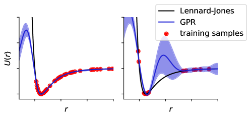
Figure 27: Using GPR to learn the Lennard-Jones potential (same as in Figure 25). Here, we trained two different GPR models: First, on the same 80 points we used for Figure 25, and then one for a bad training set with “holes”, i.e., areas from which we did not sample training points. Again, we tuned the hyperparameters of the kernel and then predicted for all points. We can observe that, similar to our KRR results, our model cannot predict the strong repulsion due to the lack of training points. But, in contrast to the KRR, the GPR gives us an estimate for the uncertainty that is larger when we lack examples in a particular region.

Up to now, we surveyed the models from a frequentist point of view in which probabilities are considered as long-run frequencies of events. A more natural framework to look at probabilities is the Bayesian point of view. Bayesian learning is built around Bayes rule³⁰⁷

$$\underbrace{P\left(\theta|D\right)}_{\text{posterior}}=\frac{\overbrace{P\left(D|\theta\right)}^{\text{likelihood}}\overbrace{P\left(\theta\right)}^{\text{prior}}}{\underbrace{P\left(D\right)}_{\text{evidence}}},$$ (17)

which describes how the likelihood $P\left(D|\theta\right)$ (probability of observing the data given the model parameters) updates prior beliefs $P\left(\theta\right)$ after observing the data $D$. This updated distribution is the posterior distribution $P\left(\theta|D\right)$ of model parameters $\theta$.

Similar to molecular Monte-Carlo simulations one can use Markov chain Monte-Carlo to sample the posterior distribution $P\left(\theta|D\right)$. Several packages like pymc3³⁰⁸ and Edward³⁰⁹ offer a good starting point for probabilistic programming in Python.

The power of Bayesian modeling is that one can incorporate prior knowledge with the choice of the prior distribution and that it allows for a natural way to deal with uncertainties as the output, the posterior distribution $P\left(\theta|D\right)$, is a distribution of model parameters. Furthermore, it gives us a natural way to compare models: The best model is the one with the highest evidence, i.e., probability of the data given the model.³¹⁰

An example of how prior knowledge can be incorporated is a work by Mueller and Ceder who incorporated physical insight to fit cluster expansions, which are simple but powerful models that express the property of system using single-site descriptors. An archetypal example is the Ising model. They used physically intuitive insights such as the distance of the prediction to a simple model, like a weighted average of pure component properties for the energy of an alloy, or that observation that similar cluster functions should have similar values, to improve the predictive power of such cluster expansions. This is effectively a form of regularization, equivalent to Tikhonov regularization (cf. section 6.2.1).

Gaussian Process Regression

Bayesian methods are most commonly used in the form of GPR,³¹¹ which drives the Gaussian approximation potentials (GAPs).¹⁹⁵ GPR is the Bayesian version of KRR, i.e., it also solves eq. 16.

In GPR one no longer uses a parametric functional form (like polynomials or a multilayer perceptron (MLP)) to model the data but uses learning to adapt the distribution (“ensemble” of functions), where the initial distribution (the prior) reflects the prior knowledge.³¹² That is, in contrast to standard (multi)linear regression one does not directly choose the basis functions but rather allows for a family of different possible functions (this is also reflected in the uncertainty band shown in Figure 27 and the spread of the functions in Figure 28).

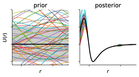
Figure 28: Samples from the prior and posterior distributions for the fit shown in Figure 27 using the same scale for the axes. Here, we assume a zero mean (thick black line) for the prior but the mean in the posterior is no longer zero after the inference. The standard deviation is shown as a gray area.

We can think of the prior distribution as samples that are drawn from a multivariate normal distribution, that is characterized by a mean $\boldsymbol{\mu}$ and a covariance $\mathbf{C}$, i.e., we can write the prior probability as

$$P(\mathbf{y})=\mathrm{Normal}(\boldsymbol{\mu},\mathbf{C})\overset{\boldsymbol{\mu}=0}{\propto}\exp\left(-\frac{1}{2}\,\mathbf{y}^{T}\mathbf{C}^{-1}\mathbf{y}\right)$$ (18)

Usually, one uses a mean of zero and the covariance matrix $\mathrm{cov}(y(x),y(x^{*}))$ that describes the covariance of function values at $x$ and $x^{*}$—i.e., it is fully analogous to the kernel in KRR. But in KRR one needs to perform a search over the kernel hyperparameters (like the width of the Gaussian), whereas the GPR framework allows learning the hyperparameters using gradient descent on the marginal likelihood, which is the objective function in GPR.

Also, the regularization term has another interpretation in GPR, as it can be thought of as noise $\sigma_{f}$ in the observation

$$\mathrm{cov}(y_{i},y_{j})=C_{ij}+\sigma_{f}\,\delta_{ij}$$ (19)

with Kronecker delta $\delta_{ij}$ (1 for $i=j$, else 0). Hence, the regularization also has a physical interpretation, whereas in KRR we introduced a hyperparameter $\lambda$ that we need to tune.

But the most important practical difference is that the formulation in the Bayesian framework generates a posterior distribution and hence a natural estimate of the uncertainty of the prediction. This is especially valuable in active learning settings (cf. section 3.3) where one needs an estimate of the uncertainty to decide whether to trust the prediction for a given point or whether additional training data are needed. This was for example successfully used by Jinnouchi et al. employing ab inito force fields derived in the SOAP-GAP framework.³¹³ During the molecular dynamics simulations of hybrid perovskites, they monitored the uncertainty of the predictions and then could switch to DFT in case the uncertainty was too high and refined the force field with this new training point. Using this approach, which is implemented in VASP 6, they could access time scales that would require years of simulations with first principle techniques.

5.2.4 Instance-Based Learning

Thinking in terms of distances to training examples, as we do in kernel methods, is also the key ingredient to the understanding of instance-based learning algorithms like $k$NN regression. Here, the learner only memorizes the training data and the prediction is a weighted average of the training data. For this reason, $k$NN regressors are said to be non-parametric—as they do not learn any parameters and only need the data itself to make predictions.

The difference between kernel learning and $k$NN is that in the case of kernel learning the prediction is influenced by all training examples and the nature of the locality is influenced by the kernel. $K$NN, on the other hand, only uses a weighted average of the $k$ nearest training examples. This limits the expressivity of the model but makes it easy to inspect and understand. As it requires that examples that are close in feature space are also close in property space, there might be problems in the case of activity cliffs³¹⁴ and per definition, such a model cannot extrapolate. Still, such models can be useful—especially due to the interpretability. For example, Hu et al. combined $k$NN with a Gaussian kernel weighting over the $k$ neighbors to predict the capacity of lithium-ion batteries.³¹⁵

An interesting extension of $k$NN for virtual high-throughput screenings was developed by Swamidass et al. The idea here is to refine the weighting of the neighbors using a small NN, which allows taking non-linearities into account.³¹⁶ The advantages here are the short training time, the low number of parameters, and hence the low risk of overfitting and the interpretability, which is only slightly lower than for a vanilla $k$NN.

5.2.5 Ensemble Methods

Ensemble models try to use the “wisdom of the crowds” by using a collection (an ensemble) of several weak base learners, which are often high-variance models like decision trees, to produce a more powerful predictor.^{317, 318}

The power of ensemble models is to reduce the variance (the error due to the finite sample, i.e., the instability of the model) while not increasing the bias of the model. This works if the predictors are uncorrelated.⁷ In detail, one finds that the variance is given by

$$\text{variance}(x)=\rho{(x)}\sigma^{2}+\frac{1-\rho(x)}{M}\sigma^{2},$$ (20)

where $M$ is the covariance matrix of the $M$ predictors with variance $\sigma$. The bias is given by

$$\text{bias}^{2}(x)={(f(x)-\mu)}^{2}.$$ (21)

These equations mean that for an infinite number of predictors ($M\to\infty$) with no correlations with each other ($\rho=0$) we can completely remove the variance and the only remaining sources of error are the bias of the single predictor and the noise. Hence, this approach can be especially valuable to improve unstable models with high variance. One example for high-variance models are decision trees (DTs) (also known as classification and regression tree (CART)) which build flow chart like models by splitting the data based on particular values of variables, i.e., based on rules like “density greater than $1\text{\,}\mathrm{g}\text{\,}{\mathrm{cm}}^{-3}$?” Only one such rule is usually not enough to describe physical phenomena, wherefore usually many rules are chained. But such deep trees can have the problem that their structure (splitting rules) is highly dependent on the training set, wherefore the variance is high. One approach to minimize this variance is to build ensemble models. Another motivation for ensemble models can be given based on the Rashomon effect which describes that there are usually several models with different functional forms that perform similarly. Averaging over them using an ensemble can resolve to some extent this non-uniqueness problem, and make models more accurate and stable.³¹⁹

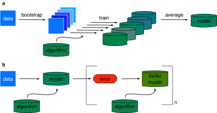
Figure 29: Schematic representation of the two most popular approaches for the creation of ensemble models, bagging (a) and boosting (b).

There are two main approaches for the creation of ensemble models (cf. Figure 29): The first one is called bagging (bootstrap aggregating) in which bootstraps of the training are fitted to a model and the predictions of all models are averaged to give the final prediction. In RFs, which are one of the most popular models in materials informatics, this idea is combined with random feature selection, in which the model is fitted only on a subset of randomly selected features. ExtraTrees, are even more randomized by not using the optimal cut at different points in the decision tree but the best one from a random selection of possible cuts.³²⁰ Additionally, they also do not use bootstraps but the original training set. In a benchmark of ML models for the prediction of the thermodynamic stability of perovskites (based on composition features) Schmidt et al. found that ExtraTrees outperform random forest, neural networks, ridge regression and also adaptive boosting (which we will discuss in the following).³²¹

The other approach for the ensembling of models is boosting. Here, models are not trained in parallel but iteratively, one after another, on the error of the previous model. The most popular learners from this category are AdaBoost³²² and gradient boosted decision treess (GBDTs) ³²³ which are efficiently (and in a refined version) implemented in the XGBoost³²⁴ and LightGBM³²⁵ libraries. Given that GBDT models are fast to train on datasets of moderate size, easy to use and robust, they are a good choice as a first baseline model on tabular descriptor data.^{326, 327} GBDTs were used in many studies on porous materials (cf. section 9). For example, they were used by Evans et al. to predict mechanical properties of zeolites based on structural properties like Si-O-Si bond lengths and angles as well as additional descriptors such as the porosity.^{328, 329}

An approach that is different from bagging and boosting is model stacking. In boosting and bagging one usually uses the same base estimator, like a DT, whereas in stacking one combines different learners and can use a meta learner to make the final prediction based on the prediction of the different models. This approach was, for example, successfully used by Wang, who could reduce the error in predicting atomization energies by $38\text{\,}\mathrm{\char 37\relax}$, compared to the best single learner, using a stacked model.³³⁰

6 How To Learn Well: Regularization, Hyperparameter Tuning, and Tricks

6.1 Hyperparameter Tuning

Almost all ML models have several “knobs” that need to be tuned to achieve good predictive performance. The problem is that one needs to evaluate the model to find the best hyperparameters—which is expensive because this involves training the model with the set of parameters and then evaluating its performance on a validation set. This problem setting is similar to the optimization of reaction conditions, where the execution of experiments is time-consuming, wherefore akin techniques are used.

The most popular way in the materials informatics community is to use grid search, where one loops over a grid of all possible hyperparameter combinations. Unfortunately, this is not efficient as all the information about previous evaluations remains unused and one has to perform an exponentially growing number of model evaluations. It was shown that even random search is more efficient than grid search, but especially Bayesian hyperparameter optimization was demonstrated to be drastically more efficient.^{331, 332} This approach is formalized in sequential model-based optimization (SMBO). The idea behind SMBO is that a (Bayesian) model is initialized with some examples and then used to select new examples that maximize a so-called acquisition (or selection) function $a$, which is used to decide which points to choose next—based on the surrogate model. The task of the acquisition function is to balance exploration and exploitation, i.e., to choose a balanced ratio between points $\mathbf{x}$ where the surrogate model is uncertain (exploration) and points where $f$, the target, is maximized (exploitation). The need for an uncertainty estimate (to be able to balance exploration and exploitation) and the ability to incorporate prior knowledge makes this task ideally suited for Bayesian surrogate models. For example, Gaussian processs (GPs) are used to model the expensive function in the spearmint³³³ and MOE (Metric Optimization Engine)³³⁴ libraries. The SMAC library³³⁵ on the other hand uses ensembles of RF, which are appealing as they naturally allow incorporating conditional reasoning.³³⁶ A popular optimization scheme is the tree-Parzen estimator (TPE) algorithm, which is implemented in the hyperopt package³³⁷ and which has an interface to the sklearn³³⁸ framework with the hyperopt-sklearn package.³³⁹ The key idea behind the TPE algorithm is to model the hyperparameter selection process with two distributions; one for the good parameters and one for the bad ones. In contrast to that, GPs and trees model it as dependent on the entire joint variable configuration. The Parzen estimator, which is a non-parametric method to estimate distributions, is used to build these distributions. To encode conditional hyperparameter choices, the Parzen estimators are structured in a tree.

6.2 Regularization

Many problems in which we are interested in the chemical sciences and materials science are ill-posed. In some cases, they are not smooth, in other cases, not every input vector is feasible (only a fraction of all imaginable compounds exist at standard conditions), and in other cases, our descriptors might not be as unique as we would want them to be, or we have to deal with noise in the data. Moreover, we often have to cope with little (and wide) data which can easily lead to overfitting. To remedy these problems one can use regularization techniques.³⁴⁰

Particularly powerful regularization techniques are based on physical or chemical insights, like the reaction tree heuristic form Rhone et al., where they only consider reaction products that are close to possible outcomes of a rule-based reaction tree.¹³⁹

In the following, we will discuss more conventional techniques that require no physical or chemical insight and that are applicable to most problems.

6.2.1 Explicit Regularization: Adding an Term or Layer

The most popular way to avoid overfitting is to add a term that penalizes high model weights (“large slopes”) to the loss function:

$$L(\mathbf{w})=\lambda\|\mathbf{w}\|^{p}.$$ (22)

In most of the cases, one uses either the Manhattan norm ($p=1$), which is known as the Lasso ($l_{1}$), or the $p=2$, which is known as ridge regularization. As we discussed previously (cf. section 4.3.2), the Lasso yields sparse solutions which can be seen as a general physical constraint.

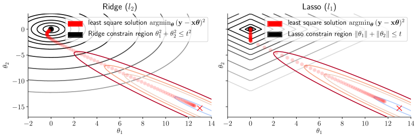
Figure 30: Visualization of the $l_{1}$ and $l_{2}$ constraints and the solution paths. The solution (dots) of the constrained optimization is at the intersection between the contours of the least square solution (red/blue colored ellipses indicating with the color the error for different parameter choices) and the regularization constraint region (black), which extent depends on $\lambda\propto 1/t$. For $\lambda=0$, we recover the least square solution, for $\lambda\to\infty$, the solution will lie at (0,0). If we increase $\lambda$, the optimal solution will tend to be zero in one dimension at the vertex of the Lasso constrain region. For the ridge case, the smooth constrain region will lower the magnitude of the weights, but will not force them to exactly zero. Figure created based on an illustration in Tibshirani, Friedman and Tibshirani³¹ and code by Sicotte.³⁴¹

Since the ridge term shrinks high weights smoothly (there are no edges in the regularization hypercube, cf. Figure 30) it does not lead to sparse solutions but it can be seen as a way to enforce smoother solutions. For example, we do expect potential energy surfaces to vary smoothly with conformational changes—a squiggly polynomial with high weights will hence be a bad solution that does not generalize. Ridge regression can be used to enforce this when training models. For both Lasso and ridge regression, we recover the original solution for $\lambda\rightarrow 0$ and force it to zero for $\lambda\to\infty$.

In DL specific regularization layers are often used to avoid overfitting. The most widely known technique, dropout, randomly disables some neurons from training.³⁴² As it is computationally cheap and can be implemented in almost any network architecture, it belongs to the most popular choices.

For trees, one usually uses pruning heuristics to limit overfitting. One can either limit the number of splits or the maximum depth of the trees before fitting them or eliminate some leaves after fitting.³⁴³ This idea was also used in NNs, e.g., by automatically deleting weights (also known as optimal brain damage (OBD)).³⁴⁴ This procedure not only improves generalization but can also speed up inference (and training).³⁴⁵

6.2.2 Implicit Regularization: More Subtle Ways to Stop the Model From Remembering

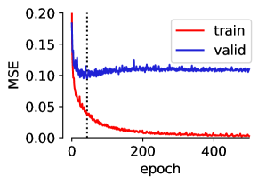
Figure 31: Example of early stopping. For this example, we trained a NN (three hidden layers with ReLU activation and 250, 100, and 10 neurons, respectively, followed by linear activation in the output layer) using the Adam optimizer,³⁴⁶ to predict the CO2 uptake for structures in the database from Boyd et al.¹³ using RACs and pore geometry descriptors as features. We can observe that after approximately 43 epochs (dotted vertical line) the training error still decreases, whereas the validation error starts to increase again.

But there are also other, more subtle ways, to avoid overfitting. One of the simplest, most powerful and generally applicable techniques is early stopping. Here, one monitors both the error on the training and a validation set over the training process and stops training as soon as the validation error no longer decreases (cf. Figure 31).³⁴⁷ Another simple and general technique is to inject noise in the training process.^{348, 349}

For the training of NN batch normalization is widely used.³⁵⁰ Here, the input to layers of a DNN is normalized in each training batch, i.e., the means and the variance are fixed in this way. It was shown that this can accelerate training but it also acts as a regularizer as each training example no longer produces a deterministic value as it depends on which batch it is in.³⁵⁰

Similarly, the training algorithm itself, batched stochastic gradient descent (SGD), was shown to induce implicit regularization due to its stochasticity as only a part of all training examples is used to approximate the gradient.^{351, 352}

In general, one finds that stochasticity is a theme underlying many regularization techniques. Either through the addition of noise, by randomly dropping layers, or by making the prediction not fully deterministic by means of batch normalization. This is in some sense similar to bagging as we also average over many slightly different models.³⁵³

7 How to Measure Performance and Compare Models

In ML, we want to create a model that performs well on unseen data for which we often do not know the underlying distribution when we train a model. To optimize our models towards good performance on unseen data we need to develop surrogates for the performance on the unseen data (empirical error estimates). An article by Sebastian Rascka gives an excellent overview (see Figure 32) of different techniques for model evaluation and selection (the mlxtend Python library of the same author implements all the methods we discuss).³⁵⁴

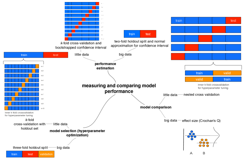
Figure 32: Model performance evaluation and comparison landscape, following the schema from Raschka.³⁵⁴. Blue boxes represent training data, red ones test data. Validation data, for hyperparameter optimization, is shown with orange boxes. Differences between groups can be shown with Gardner-Altman plots where the data for each group are shown with dots and the effect size is shown with a bootstrapped confidence interval.

Often, one finds that models are selected, compared and evaluated based on only one single number, which is the MAE in many materials informatics applications. But this might not be the optimal metric in all cases—especially since such global metrics depend on the distribution of data points (cf. Figure 33) and in materials informatics we often do not only want a model that is “on average right” but one that can also reliably find the top performers. Moreover, in some cases, we want to consider other parameters such as the training time, the feature set or the amount of training data needed. Latter we can for example extract from learning curves in which a metric for the predictive performance, like the MAE, is plotted against the number of training points.^{355, 356, 186}

The optimal (and feasible) model evaluation methodology depends on the amount of available data, the problem setting (e.g., if extrapolation ability is important) and the available computational resources. We will discuss these trade-offs in the following.

Figure 33: Influence of class imbalance on different classification metrics. For this experiment, we used different thresholds (median, mean $2.5\text{\,}\mathrm{mmol}\text{\,}{\mathrm{g}}^{-1}$) for CO2 uptake to divide structures in “high performing” and “low performing” (see histogram inset). I.e., we convert our problem with continuous labels for CO2 uptake to a binary classification problem for which we now need to select an appropriate performance measure. We then test different baselines that randomly predict the class (uniform), i.e., sample from a uniform distribution, that randomly draw from the training set distribution (stratified) and that only predict the majority class (majority). For each baseline and threshold, we then evaluate the predictive performance on a test set using common classification metrics as the accuracy (red), precision (blue), recall (yellow), F₁ score (green), and the AUC (pink). We see that by only reporting one number, without any information about the class distribution, one might be overly optimistic about the performance of a model, i.e., some metrics give rise to a high score even for only random guessing in the case of imbalanced distributions. For example, using a threshold of $2.5\text{\,}\mathrm{mmol}\text{\,}{\mathrm{g}}^{-1}$ we find high values for precision for all of our sampling strategies. Note that some scores are set to zero due to not being defined due to zero division.

7.1 Holdout Splits and Cross-Validation: Sampling Without Replacement

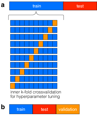
Figure 34: Comparison of model selection techniques for little and big data. For little data, one can use $k$-fold cross-validation with a separate test set (a) whereas the holdout method with three sets can be used for big data (b). In $k$-fold cross-validation the data is split into $k$ folds and one loops over all the $k$-folds, using $k-1$ folds as the training set and the $k$th fold for testing.

The most common approach to measure the performance is to create two (or three) different data sets: the training set, on which the learning algorithm is trained on, the development (or validation set), which is used for hyperparameter tuning, and the test set, which is the ultimate surrogate for the performance on unseen data (cf. Figure 34 b). We do not use the test set for hyperparameter tuning to avoid data leakage, i.e., by tuning our hyperparameters on the test we might overfit to this particular test set. The most common choice to generate these sets is to use a random split of the available data.

But there are caveats with this approach.³⁵⁴ First, and especially for small datasets, the number of training points is reduced (which introduces a pessimistic bias) in this way. But at the same time, the test set must still be large enough to detect statistically significant differences (and avoid too much variance). Second, one should note that random splitting can change the statistic, i.e., we might find different class ratios in the test set than in the training set, especially in case of little data (cf. the discussion for Figure 5).

The most common approach to deal with the first problem is $k$-fold cross-validation (cf. inner loop in Figure 34 a), which is an ensemble approach to the holdout technique. The idea here is to give every example the chance to be part of the training set by splitting the dataset into $k$ parts, using one part for the validation and the remaining $k-1$ parts for training and iterate this procedure $k$ times. A special case of the $k$-fold method is when the number of folds is equal to the number of data points, i.e., $k=n$. This case has a special name, leave-one-out cross validation (LOOCV), as it is quite useful for small datasets where one does not want to waste any data point, and it is also an almost unbiased estimator since nearly all data is used for the training. But it comes with a high computational burden and a high variance (the training set merely changes but the test example can change drastically from one fold to the next). Empirically, it was found that $k=10$ provides a good trade-off between bias and variance for many datasets.³⁵⁷ But, one needs to keep in mind that a pessimistic bias might not be a problem as in some cases, as in the model selection, we are only interested in relative errors of different models.

A remedy for the second problem of the holdout method (the change of the class distributions upon sampling) is stratification (cf. Figure 5), which is a name for the constraint that the original class proportions are kept in all sets. To use this approach in regression one can bin the data range and apply stratification on the bins.

One caveat one should always keep in mind when using cross-validation is that the data splitting procedure must be applied before any other step of the modeling pipeline (filtering, feature selection, standardization, …) to avoid data leakage. The problem of performing for example feature selection before splitting the data is that feature selection is then performed based on all data (including the test data) which can bias which features are selected (based on the information from the test set)—which is an unfair advantage.

7.2 Bootstrap: Sampling With Replacement

An alternative to $k$-fold cross-validation is to artificially create new datasets by means of sampling with replacement, i.e., bootstrapping. If one samples $n$ examples from $n$ data points with replacement, some points might not be sampled (in the limit of large data, only $63.2\text{\,}\mathrm{\char 37\relax}$ will be sampled).³⁵⁸ Those can be used as a leave-one-out bootstrap (LOOB) estimator of the generalization error and using 50–100 bootstraps, one also finds reliable estimates for confidence intervals (vide infra). Since only $63.2\text{\,}\mathrm{\char 37\relax}$ of the examples are selected also this estimator is pessimistically biased and corrections like the 0.632(+) bootstrap³⁵⁹ have been developed to correct for this pessimistic bias. In practice, the bootstrap is more complicated than the $k$-fold cross-validation for the estimation of the prediction error, e.g., because the size of the test set is not fixed in the LOOB approach. Therefore, in summary, the 10-fold cross-validation offers the best compromise for model evaluation on modestly sized datasets—also compared to the holdout method which is the method of choice for large datasets (like for DL applications).³⁶⁰

7.3 Choosing the Appropriate Regression Metric

One of the most widely known metrics is the $R^{2}$ value (for which several definitions exist, which are equal for the linear case).³⁶¹ The most basic definition of this score is the ratio between the variance of the predictions and the labels. The problem is that in this way it can be arbitrarily low even if the model is correct and e.g., on Anscombe’s quartet it has the same value for all datasets (cf. Figure 4). Hence, this metric should be used with great care. The choice between the MAE and the MSE depends on how one wants to treat outliers. If all errors should be treated equally one should choose the MAE, if large errors should get higher weights, one should choose the MSE. Often, the square root of latter, the root MSE (RMSE), is used to achieve a metric that is more easily interpretable.

To get a better estimate of the central tendency of the errors, one can use for example the median or trimean³⁶² absolute error, which is a weighted average of the median, the first quartile, and the third quartile.

Especially in the process of model development it is valuable to analyze the cases with maximum errors by hand to develop ideas why the model’s prediction was wrong. This can for example show that a particular structure class is underrepresented—in which case it might be worth generating more data for this class or to try techniques for imbalanced learning (cf. section 3). In other cases one might also realize that the feature set is inadequate for some examples or that features or labels are wrong.

7.4 Classification

7.4.1 Probabilities That Can Be Interpreted as Confidence

An appealing feature of many classification models is that they output probabilities and one might be tempted to interpret them as “confidence in the prediction”. But this is not always possible without additional steps. Ensemble models, such as random forest for example tend to rarely predict high or low probabilities.³⁶³ To remedy this, one can calibrate the probabilities using either Platt scaling or isotonic regression. Platt scaling is a form of logistic regression where the outputs of the classifier are used as input for a sigmoid function and the parameters of the sigmoid are estimated using maximum likelihood estimation on a validation set. In isotonic regression, on the other hand, one fits to a piecewise constant, stair-shaped, function which tends to be more prone to overfitting. To study the quality of the probabilities that are produced by a classifier it is convenient to plot a reliability diagram in which the probabilities are divided into bins and plotted against their relative frequency. A well-calibrated classifier should fall onto the diagonal of this plot.

7.4.2 Choosing the Appropriate Classification Metric

Especially in a case in which one wants to identify the few best materials, accuracy—although widely used—is not the ideal classification metric. This is the case as accuracy is defined as the ratio of correct predictions over the total number of predictions and can, in the case of imbalanced classes, be maximized by always predicting the majority class—which certainly is not the desired outcome (cf. Figure 33). Popular alternatives to the accuracy are precision and recall:

accuracy $$=\frac{\text{true positive}+\text{true negative}}{\text{true positive}+\text{true negative}+\text{false positive}+\text{false negative}}$$ (23)

precision $$=\frac{\text{true positives}}{\text{true positives}+\text{false positives}}$$ (24)

recall $$=\frac{\text{true positives}}{\text{true positives}+\text{false negatives}}.$$ (25)

The precision will be low when the model classifies many negatives as positives and the recall, on the other hand, will be low if the model misses many positive results. Similar to accuracy these metrics have their issues, e.g., recall can be maximized by predicting only the positive class. But as there is usually a trade-off between precision and recall, summary metrics have been developed. The $F_{1}$ score tries to summarize precision and recall using a harmonic mean

$$F_{1}=\frac{2}{\frac{1}{\text{precision}}+\frac{1}{\text{recall}}}=2\,\frac{\mathrm{precision}\cdot\mathrm{recall}}{\mathrm{precision}+\mathrm{recall}},$$ (26)

which is useful for imbalanced data.

Since the classification usually relies on a probability (or score) threshold (e.g., for binary classification we could treat all predictions with probability $>0.3$ as positive), receiver-operating characteristic (ROC) curves are widely used. Here, one measures the classifier performance for different probability thresholds and plots the true positive rate [true positives / (true positives + false negatives)] against the false positive rate $[1-\mathrm{true\ negative}/(\mathrm{true\ negative}+\mathrm{false\ positive})]$. A random classifier would fall on the diagonal of a ROC curve and the optimal classifier would touch the top left corner (only true positives). This motivated the development of metrics that try to capture the full curve in only one number. The most popular one is the AUC,^{364, 365} but also this metric is no silver bullet. For example, care has to be taken when one wants to use the AUC as a model selection criterion. For instance, the AUC will not carry information about how confident the models are in their predictions—which would be an important for model selection.³⁶⁶

Related to ROC curves are precision-recall curves. They share the recall (true positive rate) with the ROC curves but plot it against the precision, which is, for a small number of positives, more sensitive to false positive predictions than the false positive rate. For this reason, we see an increasing difference between the ROC and the precision-recall curves with increasing class imbalance (cf. Figure 35).³⁶⁷

Figure 35: Comparison of precision-recall (top) and ROC (bottom) curves for different thresholds for the binary classification of CO2 uptake (same as for Figure 5). For this example, we fitted a GBDT classifier on the dataset from Boyd et al.¹³ We can observe that for increasingly imbalanced class distributions (e.g., higher threshold for “high” performing MOFs, i.e., there are few of them) the difference between the shape of the precision-recall curve and the ROC, as well as the area under those curves, are more different. For imbalanced classes, the precision-recall curve (and the area under this curve) is a more sensible measure of model performance.

Usually, it is also useful to print a confusion matrix in which the rows represent the actual classes and the columns the predicted ones. This table can be useful to understand between which classes misclassification happens and allows for a more detailed analysis than a single metric. A particularly useful Python package is PyCM which implements most of the classification metrics, including multi-class confusion matrices.³⁶⁸

7.5 Estimating Extrapolation Ability

For some tasks, like the discovery of new materials, one wants models that can robustly extrapolate. To estimate the extrapolation ability, specific metrics have been developed. The leave-on-cluster-out cross-validation (lococv) technique proposed by Meredig et al. is an example of such a metric.³⁶⁹ The key idea is to perform clustering in the $n$ cross-validation runs and leave one of the clusters out in the training set and then use this cluster as the test set. Xiong et al. propose a closely related approach: But instead of clustering the data in feature space they partition the data in target property space and use only a part of property space for training in a $k$-fold cross-validation loop and the holdout part for testing purposes.³⁷⁰

Similar to that is the scaffolding splitting technique,³⁶⁷ in which the two-dimensional framework of molecules³⁷¹ is used to separate structurally dissimilar molecules into training and test set.

7.6 Domain of Applicability

In production, one would like to know if the predictions the model gives are reliable. This question received particular attention in Cheminformatics^{372, 373} with the emphasis of the registration evaluation and authorization of chemicals (REACH) regulations on the reliability of QSAR predictions.^{374, 375, 376} Often, comparing the training and production distributions is a good starting point to understand if a model can work. Here, one could first consider if the descriptor values of the production (test) examples fall into the range of the descriptors of the training examples (boundary box estimate). This approach gives a first estimate if the prediction is made on solid ground, but it does not consider the distribution of the training examples, i.e., it might overlook “holes” in the training distribution.³⁷² But it is easy to implement and can, for example, be used during a molecular simulation with a NN potential. If a fingerprint vector outside the bounding box is detected, a warning could be raised (or the ab initio data can be calculated in an active learning setting).²⁹¹

More involved methods often use clustering,³⁷⁷ subgroup discovery,³⁷⁸ and distances to the nearest neighbors of the test datum. If this distance is greater than a threshold, which can be based on the average distance of the points in the training set, the model can be considered unreliable. Again, the choice of the distance metric requires some testing.

More elaborate are methods based on the estimation of the probability density distribution of datasets and the evaluation of their overlaps. These methods are closely related to kernel-mean matching (KMM)—a method to mitigate covariate shift—which attempts to estimate the density ratio between test (production) and training distribution and then reweights the training distribution to more closely resemble the test (or production) distribution.³⁷⁹

7.7 Confidence Intervals and Error Estimates

The outputs of ML models are random variables, with respect to the sampling, e.g., how the training and test set are created (cf. sections 3.2 and 6)³⁸⁰ and the optimization (one may end up in a different local minimum for stochastic minimization) and in some cases also with respect to the initialization. Hence, one needs to be aware that there are errorbars around the predictions of any ML model that one needs to consider when comparing models (cf. section 7.8), using the predictions, or simply to estimate the stability of a learning algorithm.

In addition, reliable error estimates are also needed to make predictions based on ML models trustworthy. Bayesian approaches automatically produce uncertainty estimates (cf. section 5.2.3) but are not applicable to all problem settings. In the following, we will review techniques that can be used to get error estimates in a model-agnostic way.

7.7.1 Ensemble Approach

Based on the insight that the outputs are random variables it seems natural to use an ensemble approach to calculate error bars.³⁸¹ One of the most popular ways to do this is to train the same model on different bootstraps of the dataset and then take the variance of this ensemble as a proxy for the error bars. This is connected to two insights. First, the training set is only one particular realization of a probability distribution (which is the key idea behind the bootstrap), and second, the variance of the ensemble will be larger for cases in which the model is uncertain and has seen few training data.³⁸²

A related approach is to use to same data but to vary the architecture of the model, e.g., the number of hidden layers. If the variance between the predictions in a particular part of chemical space is too large, this indicates that the models are still too “flexible” and need more training data in that particular region.²⁹¹ In contrast to the bootstrap approach, the ensemble surrogate can also be used in production, i.e., when we do not know the actual labels.

The fact that all ensemble or resampling approaches increase the computational cost motivated the development of other approaches for uncertainty quantification.

7.7.2 Distance-based

Most of the distance-based uncertainty surrogates are based on the idea that there is a relationship between the distance of a query example from the training set and the uncertainty of the prediction. This is directly related to the concept of the domain of applicability, which we discussed above (cf. section 7.6). Although this approach may seem straightforward, there are caveats as the feature vector and the distance metric must be carefully chosen to allow for the calculation of a meaningful distance. Also, this approach is not applicable to models that perform representation learning (cf. section 5.1.1).

This motivated Kulik and co-workers to develop uncertainty estimators that are cheaper than ensemble approaches and applicable to NN in which feature engineering happens in the hidden layers.³⁸³ The idea of this approach is to use the distance in the latent space of the NN, which is calibrated by fitting it to a conditional Gaussian distribution of the errors, as a surrogate for the uncertainty.

7.7.3 Conformal Prediction

A less widely known technique is conformal prediction, which is a rigorous mathematical framework that only assumes interchangeability (which is the case for independently and identically distributed (i.i.d) data, which is usually assumed for interpolative applications of ML) and can be used for any learning framework with minimal cost. Practically, given a test datum $x_{i}$ and a significance level of choice $\epsilon\in(0,1)$, a conformal predictor calculates a prediction region $\Gamma_{i}^{\epsilon}\subseteq Y$ that contains the ground truth $y_{i}\in Y$ with a probability of $1-\epsilon$.

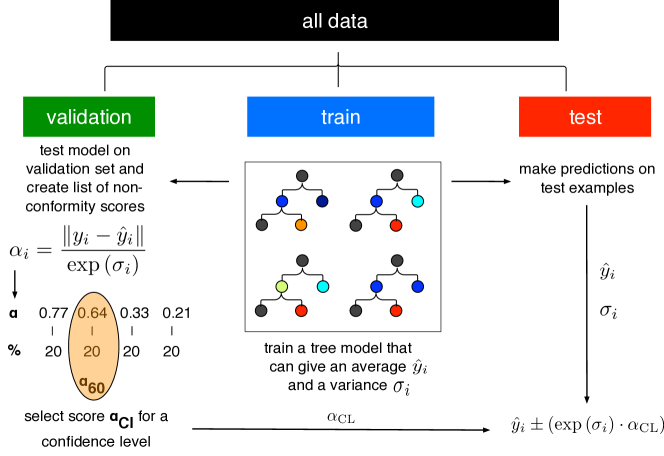
Figure 36: Example of inductive conformal prediction for the regression with tree models.

The idea behind this concept (cf. Figure 36) is to compute the nonconformity scores that measure the “uniqueness” of an example, using a nonconformity function, that can be the MAE ($\|y_{i}-\hat{y}_{i}\|$) for regression,³⁸⁴ on a calibration set (green in Figure 36)

$$\alpha=\frac{\|y_{i}-\hat{y}_{i}\|}{\exp\left(\sigma_{i}\right)},$$ (27)

and that can be scaled by a measure of uncertainty, like the variance $\sigma$ between the different trees in a random forest.^{385, 386} One then sorts this list of nonconformity scores and can then choose the $n$th percentile (e.g., 60th percentile $\alpha_{\mathrm{CL}}$ corresponding to a confidence level of $60\text{\,}\mathrm{\char 37\relax}$) and compute the prediction region for a test example (red in Figure 36)

$$\hat{y}_{i}\pm\left(\exp\left(\sigma_{i}\right)\cdot\alpha_{\mathrm{CL}}\right).$$ (28)

The review by Cortés-Ciriano and Bender gives a more detailed overview of the possibilities and limitations of conformal prediction in the chemical sciences, especially for drug discovery,³⁸⁶ and a tutorial by Shafer and Vovk provides more theoretical background.³⁸⁷ A Python package that implements the conformal prediction framework is nonconformist.³⁸⁸

7.8 Comparing Models

One of the reasons why we focus on developing robust metrics and measures of variance is to be able to compare the predictive performance of different models. Even though, as it is sometimes done, one could simply compare the metrics, such a comparison is not meaningful given that the predictions are random variables with an error bar around them. The task of the modeler is to identify statistically significant and relevant differences in model performance. There are a range of statistical tools that try to identify significant differences.³⁸⁹ Some of the fallacies and the most common techniques are discussed in a seminal paper by Dietterich.³⁸⁹

If the difference between the error of two models is small, or not even statistically significant, one usually prefers, following Occam’s Razor, the simpler model. One popular rule-of-thumb is the one-standard error rule according to which one chooses the simplest model within one standard error of the best performing one.^{354, 31}

The simplest approach to compare two models is to perform a $z$-test which practically means to check if their confidence intervals overlap—but this tends to often show differences even if there are none (due to not independent training and/or test sets in resampling approaches which results in a variance estimate that is too small).

It was found that one of the most reliable estimates is the $5\times 2$-fold cross-validated $t$-test in which the data is split into training and test set five times. For each fold, the two models that shall be compared are fitted on the training set and evaluated on the test set (and the sets are rotated afterward) which results in two performance difference estimates per fold. The variance of this procedure can be used to calculate a $t$-statistic which was shown to have a low type-1 error—but also low replicability, i.e., different results are obtained when the test is rerun.³⁹⁰ Using statistical tests for model comparison leads to another problem when one does not only compare two models: Namely, the problem of multiple comparisons for which reasons additional corrections, like the Bonferroni correction, need to be applied. Also, problems with the interpretability of $p$-values are also widely discussed outside the ML domain. For this reason, it is not practical to use such statistical tests and estimation statistics might be the method of choice.^{391, 392, 392, 393} It is more meaningful to compare effect sizes, e.g., differences between the accuracies of two classifiers, and the corresponding confidence interval than relying on a dichotomous decision based on the $p$-value. A convenient format to do this can be a Gardner-Altman plot for bootstrapped performance estimates. Here, each measurement is plotted together with the means and the bootstrapped confidence interval of the effect size—with is particularly useful if the main focus of a study is to compare algorithms. A Python package that create such plots is DABEST.³⁹⁴

7.8.1 Ablation Studies

When designing a new model, one often changes multiple parameters at the same time: the network architecture, the optimizer or the hyperparameters. But to understand what caused an improvement, ablation studies, where one removes one part of the set of changes and monitors the change in model performance, can be used. In several instances, it was shown that not a more complex model architecture but rather a better hyperparameter optimization is the reason for improved model performance.^{395, 396, 397} Understanding and reporting where the improvement stems from is especially important when the main objective of the work is to report a new model architecture.

7.9 Randomization Tests: Is the Model Learning Something Meaningful?

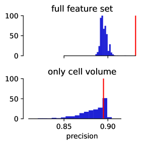
Figure 37: Example of a $y$-scrambling analysis to assess the significance of a performance metric. For this example, we built two simple GBDT classifiers that attempt to classify the materials from Boyd et al.¹³ into structures with high and low CO2 uptake, respectively. We trained one of them using RACs and pore property descriptors and the other one using only the cell volume as descriptor. We also measure the performance using the AUC and can observe that the model, trained on the full feature set, can capture a relationship in the real data (red line) and significantly ($p<0.01$) outperforms the models with permuted labels (bars). The model trained only on the cell volume does not perform better than random.

With the number of tested variables the probability of chance correlation increases—but ideally, we want a meaningful model. Randomization tests, where either the labels or the feature vectors are randomized, are powerful ways to ensure that the model learned something for the right or at least reasonable reasons. $y$-scrambling,³⁹⁸ where the labels are randomly shuffled is hence known as the “probably most powerful validation strategy” for QSAR (cf. Figure 37).³⁹⁹ A web app available at go.epfl.ch/permutationplotter allows performing basic permutation analysis online and to explore how easy it is to generate “patterns” using random data. The importance of randomization tests has recently been demonstrated for a model for C-N cross-coupling reactions.⁴⁰⁰ Chuang and Keiser showed that “straw” models which use random fingerprints perform similarly to the original model trained on chemical features.⁴⁰¹ This showcases that randomization tests can be a powerful tool to understand if the model learns causal chemical relationships or not.

8 How to Interpret the Results: Avoiding the Clever Hans

Clever Hans was a horse that was believed to be able to perform intellectual tasks like arithmetic operations (it was later shown that it did this by observing the questioner). In ML, there is also the risk that the user of a model can be deceived by the model and (unrightfully) believe that a model makes predictions based on physical or chemical rules it (supposedly) learned.⁴⁰² In the following, we describe methods that can be used to avoid “black boxes” or to at least peek inside them to debug models, understand problems with the underlying dataset or to extract design rules. This is especially valuable when high-level, physical and interpretable, features are used.

Unfortunately, the term “interpretable” is not well-defined.⁴⁰³ Sometimes, the term might be used to describe efforts to understand how the model works (e.g., if one could replicate what the model does using pen and paper) and in other instances it might be used to generate post-hoc explanations that one could hope to use for inferring general design rules. Still, one needs to keep in mind that we draw conclusions and interpretations only based on the model’s reasoning (and the underlying training data) which can be a crude approximation of nature and without prove of predictive ability of the underlying models, such analyzes remain inutile.³¹⁹ For a more comprehensive overview over the field of interpretable ML we recommend the book from Molnar.⁴⁰⁴

8.1 Consider Using Explainable Models

Cynthia Rudin makes a strong point against post-hoc explanations.²⁹ If they were completely faithful, there would be no need for the original model in the first place. Especially for high-stakes decisions a post-hoc explanation that is right $90\text{\,}\mathrm{\char 37\relax}$ of the time is not trustworthy. To avoid such problems, one can attempt to first use simple models that might be intrinsically interpretable, e.g., in terms of their weights. Obviously, simple models such as linear regression reach their limitations of expressivity for some problems, especially if the feature sets are not optimal.

Generalized additive models (GAMs) try to combine the advantages of linear models—for each feature one can analyze the weight (due to the additivity) and get confidence intervals around it—with flexibility to describe non-linear patterns (cf. Figure 38). This can be achieved by using the features via smooth, nonparametric functions, like splines:

$$g(E_{Y}(y|x))=\beta_{0}+f_{1}(x_{1})+f_{2}(x_{2})+\cdots+f_{p}(x_{p}).$$ (29)

GAMs are hence additive models that describe the outcome by adding up smooth relationships between the target and the label. Linear models can be seen as special case of GAMs, where the $f$ are restricted to be linear.

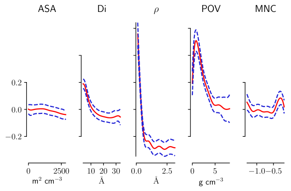
Figure 38: Examples for the splines for features that we used in a GAM to predict the N2 uptake for structures in the database of Boyd et al.¹³ Overall, we can observe that the surface area (ASA) and the minimum negative charge (MNC) have only a small influence on the prediction, whereas an increase in density leads to a stark decrease in the model outcome.

One drawback of such additive models is that interaction effects have to be incorporated by creating a specific interaction feature like $f(\text{density}\cdot\text{surface area})$ (in case one assumes that the interaction between the density and the surface area is important). A modification of Caruana et al. includes pairwise interactions in the form of $f(x_{1},x_{2})$ by default,⁴⁰⁵ and is implemented in the interpret package.⁴⁰⁶

Similar to DT—which we do not recommend due to their instability, and the fact that they are only interpretable when they are short—decision rules formulate if-then statements. The simplest approach to create such rules is to discretize continuous variables and then create cross tables between feature values and model outcomes. Afterwards, one can attempt to create decision rules based on the frequency of the outcomes, e.g., “if $\rho>$2\text{\,}\mathrm{g}\text{\,}{\mathrm{cm}}^{-3}$$ then deliverable capacity low and if $$1\text{\,}\mathrm{g}\text{\,}{\mathrm{cm}}^{-3}$<\rho<$2\text{\,}\mathrm{g}\text{\,}{\mathrm{cm}}^{-3}$$ then deliverable capacity high”. Further developments provide safeguards against overfitting and multiple features can be taken into account by deriving rules from small DT. One of the main disadvantages of this method is that it needs discretization of features and targets, which induces steps in the decision surfaces. The skater Python library implements this technique.⁴⁰⁷ Short DTs are also used in the RuleFit algorithm.⁴⁰⁸ Here, Friedman and Popescu propose to create a linear model with additional features that have been created by decomposing decision trees. The model is then sparsified using the Lasso. The problem using this approach is that, although the features and rules themselves might be interpretable, there might be problems in combining them when there are overlapping rules. This is the case since the interpretation of weights of linear models assumes that all other weights remain fixed (e.g., there can be problems with co-linear features).

Another form of interpretability can be achieved using $k$NN models. As the model does not learn anything (cf. section 5.2.4) the explanation for any prediction are the $k$ closest examples from the training set—which works well if the dimensionality is not too high (cf. section 4.1).

This also illustrates the two different levels of interpretation one might aim for. Some methods like the coefficients of linear models or the feature importance rankings for tree models (see below) give us global interpretations (integrated over all data points), whereas other techniques like $k$NN give us local explanations for each sample and some techniques can give us both (like SHapley Additive exPlanations (SHAP), see below).

8.2 Post-Hoc Techniques to Shine Light Into Black Boxes

The most popular approach to extract interpretation from ML models in the materials informatics domain is to use feature importance—often based on where in a tree model a feature contributed to a split (an early split is more important) or how good this split was, e.g., by measuring how much it reduces the model’s variance. Most of these methods fall under the umbrella of sensitivity analysis,^{409, 410} which is also widely known as the study of how uncertainty in the output of models is related to the uncertainties in the inputs by studying how the model reacts to changes in the input. Unfortunately, there are problems with several of those techniques—like the fact that some of them are biased towards the high-variance features.^{411, 412}

There are several model-agnostic alternatives that attempt to avoid this problem. Isayev et al. used partial dependence plots (cf. Figure 39) to interrogate the influence of the features and their interaction on the model outcome.²¹⁰

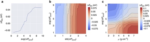
Figure 39: Partial dependence plots of $\Delta\mathrm{IP}_{\mathrm{bond}}$. The first plot reflects physical intuition that more polar bonds (larger ionization potential difference) have larger band gaps. Interactions between two features are shown in b and c. For example, we can observe that materials with higher density, $\rho$, and lower average $\Delta\mathrm{IP}_{\mathrm{bond}}$ statistically have a larger band gap. Figure reprinted from Isayev et al.²¹⁰

This can be done by marginalizing over all the other features $x_{c}$ which are not plotted:

$$\hat{f}_{x_{s}}(x_{s})=\int\hat{f}(x_{s},x_{c})\,\mathrm{d}\mathbb{P}(x_{c}).$$ (30)

The integral over all the other features $x_{c}$ is in practice estimated using Monte-Carlo (MC) integration. By integration over all but two variables, one can generate heatmaps that show how the target property varies as a function of the features assuming that those features are independent of all the other features. The latter assumption is the biggest problem with partial dependence plots.

Another powerful method, the permutation technique, shares this problem. In the permutation technique one tries to estimate the global importance of features by measuring the difference between the error of a model trained with fully intact feature columns and one where the values for the feature of interest are randomly permuted. To remedy issues due to correlated features⁴¹³ one can permute them together. The permutation technique was for example used by Moosavi et al. to capture the importance of synthesis parameters in the synthesis in the of HKUST-1.²¹

One technique that attempts to provide consistent interpretations, avoiding most of the aforementioned problems, on both local and global level is the use of Shapley values. The idea is based on a game-theoretical problem in which one wants to estimate the optimal payout for a player. The players in the case of ML are the features. Again, this involves marginalization over all the features we are not interested in but considering all possible ways in which the feature can enter the model (similar to all possible teams a player could be in). But considering all possible combinations of features is computationally unfeasible wherefore Lundberg and Lee developed new algorithms to calculate it efficiently (exact for trees and approximate for kernel methods, see Figure 40 for an example).^{414, 415, 416} In contrast to partial dependence plots, which show average effects, the plots of the feature values against the importance will appear dispersed in the case of the Shapley technique, which can give more insight into interaction effects. This technique started to find use in materials informatics. For example, Korolev et al. used SHAP values to probe their ML model for partial charges of MOFs. There they, for example, find that the model (a GBDT) correctly recovers that the charge should decrease with increasing electronegativity.⁴¹⁷ But it also highlights that (post-hoc) interpretability methods are not the only puzzle-stone towards interpretability. If the features themselves are not intuitive quantities (like the RDF) no post-hoc interpretability technique will make it easier to create design rules—but it still can be useful for debugging of models.

Still, one should keep in mind that it has also been shown that there can be stability problems with SHAP.⁴¹⁸

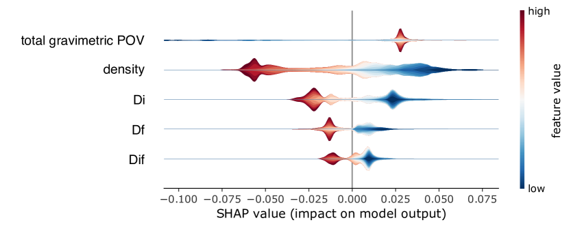
Figure 40: Summary plot of SHAP feature importance for a GBDT model, trained using pore properties descriptors (POV: pore occupiable volume, D_i: diameter of the largest included sphere, D_f: diameter of the largest free sphere, $D_{if}$: diameter of the largest included sphere along the free path) to predict N2 uptake from the CO2/N2 mixture data from Boyd et al.¹³ Note that we chose the N2 uptake as one expects that the pore geometry is more important than the chemistry, which simplifies the example. The violins in this plot show the distributions of the importance, i.e., the spread of the SHAP values (along the abscissa) and how many samples we have for different SHAP values (the thickness of the violin). The coloring encodes the value of the features, red meaning high feature values whereas blue represents low feature values (e.g., high vs. low density). The SHAP value is shown on the abscissa and reflects how a particular feature (one feature per row) with a value represented by the color impacts the prediction. For example, a high density (red color in the second row) leads to lower predictions for N2 uptake (indicated by negative SHAP values).

For NNs techniques that analyze the gradients are popular. The magnitude of the partial derivative of the outputs with respect to the input was for example also used by Esfandiari et al. to assign importance values to the features they used for their NN that predicts the CO2/CH4 separation factor.⁴¹⁹

Related is work by Umehara et al. who used gradient analysis to visualize the predictions of neural networks and showed that this analysis can reveal structure-property relationships for the design of photoanodes.⁴²⁰ This technique, where one calculates the partial derivative in the $i$th feature dimension for the $j$th sample

$$G_{ij}=\left|\frac{\partial f(\mathbf{x})}{\partial x_{i}}\right|,$$ (31)

is also known as saliency mapping. Thanks to libraries like tf-explain⁴²¹ and keras-vis⁴²² appealing visualizations of model explanations are often only one function call away, but one should be aware that there are many caveats wherefore some sanity checks (like randomization tests or addition of noise) should be used before relying on such a model interpretation.^{423, 418}

8.3 Auditing Models: What Are Indirect Influences?

In the mainstream ML community algorithmic fairness, e.g., to prevent racial bias, is a pressing problem. One might expect that this is not a problem in scientific datasets. Jia et al. showed that also reaction datasets are anthropogenically biased, e.g. by experimenters selecting reactants and reaction conditions that they know to work (Matthew effect mechanism⁴²⁴)—which is similar to the bias towards certain reaction types which Schneider et al. found in the U.S. patent database.⁴²⁵ Jia et al. trained ML models on randomly selected reaction conditions and on larger, human-selected reaction conditions from the chemical literature and found that the models trained on random conditions outperform the models trained on (anthropogenically biased) conditions from the literature for the prediction of crystal formation of amine-templated metal oxides—due to a better sampling of feature space.⁴²⁶

Some features in our feature set might encode such anthropogenic biases. Auditing techniques, as for example implemented in the BlackBoxAuditing package,⁴²⁷ try to estimate such indirect influences. In a high-stake decision case, an example for indirect influence might be a zip-code feature that is a proxy for ethnicity—which we then should drop to avoid that our model is biased due to the ethnicity.

In scientific datasets, such indirect influences might stem from artifacts in the data collection process or non-uniqueness of specific identifiers (which could be interpreted in different ways by different tools).⁴²⁸ The estimation of indirect influences works by perturbing a feature in such a way (typically by random perturbation) that it no longer can be predicted by the other features. Similar to the perturbation techniques discussed above for (direct) feature importance, one then measures the drop in performance between the original model and the one with the perturbed feature. And indeed Jia et al. found the indirect feature importance for models trained for the reaction conditions in literature conditions to be linearly correlated to those for models trained on randomly selected conditions—except for the features that describe the chemistry of the amines.⁴²⁶

9 Applications of Supervised Machine Learning

As we mentioned in the introduction, ML in the field MOFs, COFs, and related porous materials relies on the availability of tens of thousands experimental structures,^{2, 3} and to a large extent on the large libraries of (hypothetical) structures that have been assembled and scrutinized with computational screenings.^{5, 429, 430, 431, 432, 13, 433} But even with the most efficient computational techniques, like force-field-based simulations, the total number of materials has become so large that it is prohibitive to screen all possible materials for any given application. In addition, brute force screening is not the best way to uncover structure-property relationships. More importantly, other phenomena, especially electronic properties or fuzzy concepts such as synthesis or reactivity, are so complex that there is no good theory to describe the phenomenon (reaction outcomes) or that the theory is too expensive for a large-scale screening (electronic phenomena). For these reasons, researchers started to employ (supervised) ML for porous materials.

In Table LABEL:tab:overview_table we give an overview of the techniques which we discussed in the first part and some examples where they have been used in the field of porous materials and will discuss those examples in more detail in the following. It is striking that many of the techniques that we discussed in the first part did not find an application for porous materials. We discuss those possibilities in more detail in the following and the outlook.

Table 2: Overview of learning methods that we discussed in Section 5 and examples of their use in the field of porous materials. For some methods there has been no application reported in the field of porous materials, and we instead provide ideas of possible applications.

method	section	application to porous materials
representation learning
HDNNP	5.1.1	trained on fragments for MOF-5 by Behler and co-workers287
message-passing NN	5.1.1	not used for porous materials so far
convolutional or recurrent NN	5.1.1	Wang et al. used CNN to classify MOFs based on their XRPD pattern135
crystal-graph based models	5.1.1	Korolev et al. use them to predict bulk and shear moduli of pure silica zeolites and Xe/Kr selectivity of MOFs 434
generative models	2.1.2	ZeoGAN by Kim and co-workers435 (cf. section 9.7)
classical statistical learning
linear models	5.2.1	predicting gas uptakes based on tabular data of simple geometric descriptors247
kernel methods	5.2.2	predicting gas uptakes based on graphs and geometric properties,436 might be also interesting in the SOAP-GAP framework, as work by Ceriotti and co-workers as well as Chehaibou et al. showed437, 438
ensemble models	5.2.5	often used in form of RF or GBDT to predict gas uptakes based on tabular data of simple geometric descriptors, ensemble used to estimate uncertainty when predicting oxidation states439
Bayesian methods	5.2.3	have been used e.g., in the form of GPR 436 or Bayesian NN 440, 441 but not all features, like the uncertainty measure, have been fully exploited so far. This might be useful for active learning, e.g. for MD simulations in the Bayesian formulation of the SOAP-GAP framework
TDA	4.2.2	Moosavi, Xu et al. built KRR models for gas uptake in porous organic cages,185 or Zhang et al. for gas uptake in MOF 234, Lee et al. for similarity analysis238
other ML techniques
automated machine learning	10.1	Tsamardinos et al.442 use the Just Add Data tool to predict the CH4 and CO2 capacity of MOFs, Borboudakis et al. use the same tool to predict CO2 and H2 uptakes172
data augmentation	3	Wang et al. used it for the detection of MOFs based on their diffraction patterns135
transfer learning	10.3	He et al. used it for the prediction of band gaps246
active learning	3.3	could be used for MD simulations using ML forcefields313, or to guide the selection of next experiments or computations
capturing the provenance of ML experiments	10.2	Jablonka et al. used comet.ml to track the experiments they ran for building models that can predict the oxidation state of metal centers in MOFs 439
$\Delta$-ML	10.3	Chehaibou et al. used a $\Delta$-ML approach to predict random phase approximation (RPA) adsorption energies in zeolites438

9.1 Gas Storage and Separation

Gas storage is one of the simplest screening studies. Most screening studies focus on designing a material with the highest deliverable capacity, which is defined as the difference between the amount of gas a material can adsorb at the high, charging, pressure minus the amount of gas that stays in the material at the lowest operational pressure.⁴⁴³ Hence, these screening studies typically require two data points on the adsorption isotherms. Most of the studies for gas storage have focused on methane^{444, 445, 446, 447, 430, 443} and hydrogen.^{448, 446, 449}

Gas separations are another important application of porous materials^{450, 451}. Given the importance of reducing CO2 emission,^{452, 453} a lot of research has focused on finding materials for carbon capture, both experimentally^{454, 455, 456, 457} as well as by means computational screening studies.^{458, 15, 459} Gas separations require the (mixture) adsorption isotherms of the gases one would like to separate. In most screening studies, the mixture isotherms are predicted from the pure component isotherms using ideal adsorbed solution theory. For gas separations, the objective function is less obvious. Of course, one can argue that for a good separation the selectivity and working capacity are important, but one often has to carry out a more detailed design of an actual separation process to find what are the key performance parameters one would like to screen.

Most screening studies focus on thermodynamic properties. Yet, if the diffusion coefficients of the gases that need to be adsorbed are too low, excellent thermodynamic properties are of little use. Therefore, it is also important to screen for transport properties. However, only a few studies have been reported that study the dynamics.^{460, 461, 462, 463} The conventional method to compute transport properties, like diffusion coefficients, is molecular dynamics. However, depending on the value of the diffusion coefficients these simulations can be time-consuming.⁴⁶¹ Because of these limitations, free energy-based methods have been developed to estimate the diffusion coefficients from transition state theory (cf. ref. ⁴⁶², ⁴⁶³).

A popular starting point is methane storage, a topic which has been studied extensively.^{444, 445} As in most of the screening studies methane is considered a united atom without net charge, and without dipole or quadruple, the interactions with the framework atoms are described by the Van der Waals interactions.⁴³⁰ As these interactions do not vary much from one atom in the framework to another, one can expect that methane storage is dominated by the pore topology rather than the specific chemistry. Hence, most of the ML models are trained using simple geometric properties such as the density, the pore diameter or the surface area. These characteristics are obviously directly related to physisorption, but sometimes multicolinear, which can lead to problems with some algorithms as we discussed above (cf. section 4.3.3).

For gases like CO2 or H2O, the specific chemistry of the material will be more significant. For these gases, the pore geometry descriptors will not be sufficient and we will need descriptors that can describe phenomena that involve specific chemical interactions. One also has to keep in mind that conventional high-throughput screenings can have difficulties to properly describe the strong interactions of CO2 with open metal sites (OMSs).⁴⁶⁴ For example, especially for the low-pressure regime of the adsorption isotherm of CO2, the method used to efficiently (i.e., avoiding DFT calculations for each structure) assign partial charges to the framework atoms can lead to systematic errors in the results.

One also needs to realize that descriptors that are only based on geometric properties have limited use for materials’ design. Even if we find a model that relates pore properties with the gas uptake and then use optimization tools (like particle swarm optimization, genetic algorithms or random searches⁴³⁶) to maximize the uptake with respect to the pore properties there still remains the burden of proof as a given combination of pore properties might optimize gas adsorption in our model but might not be feasible or synthesizable (cf. section 3.1).

9.1.1 Starting on Small Datasets

As in other fields of chemistry, ML for porous materials developed from quantitative structure property relationship (QSPR) on small datasets (tens of data points) to the use of more complex models, such as neural networks, on large datasets with hundred thousands of data points. Generally, one needs to keep in mind that all boundaries or trends that are observed in QSPR studies can either be due to underlying physics or limitations of the dataset, which necessarily does not explore some areas of the enormous design space of MOFs.⁴⁶⁵

As in computer aided drug design (CADD), the first studies also used high-level descriptors. Kim reported one of the first QSPR for gas storage in MOFs.⁴⁶⁶ Inspired by previous works in CADD, they calculated descriptors like the polar surface area and the molar refractivity but also used the iso-value of the electrostatic potential to create a model for the H2 adsorption capacity of ten MOFs. Similar to that, Amrouche et al. built models based on descriptors of the linker chemistry of zeolitic imidazolate frameworks (ZIFs), like the dipole moment, as well as descriptors of the adsorbing gas molecules to predict the heat of adsorption for 15 ZIFs and eleven gas molecules.⁴⁶⁷ Also Duerinck et al. used descriptors like polarizability and dipole moment, which are familiar from cheminformatics, to build a model for the adsorption of aromatics and heterocyclic molecules on a set of 22 functionalized MIL-47 and found that polarizability and dipole moment are the most important features.⁴⁶⁸

Pore Geometry Descriptors

Sezginel et al. used a small set of 45 MOFs and trained multivariate linear models to predict the methane uptake based on geometric properties,⁴⁶⁹ and also Yilidz and Uzun used a small set of 15 structures to train a NN to predict methane uptakes in MOFs based on geometric properties.⁴⁷⁰ Wu et al. increased the number of structures in their study to 105 and built a model that can predict the CO2/N2 selectivity of MOF based on the heat of adsorption and the porosity.⁴⁷¹ They used this relationship to create a map of the interplay between the porosity and the heat of adsorption and their impact on the selectivity which showed that simultaneously increasing the heat of adsorption while decreasing the porosity is a route to increase selectivity for this separation.

9.1.2 Moving to Big Data

Development of New Descriptors

Fernandez et al. started working with considerably larger sets of structures and also introduced more elaborate techniques like DT or SVMs, which reflect the shift from cheminformatics with (multi)linear models on small datasets to complex nonlinear models trained on large datasets, that also other fields of chemistry experienced.²⁴⁷

In their first work,²⁴⁷ they used geometric descriptors such as the density or the pore volume to predict the methane uptake but then realized²²⁰ the need to introduce more chemistry to build predictive models for carbon dioxide adsorption. They did so by introducing the atomic property (AP) weighted RDF (AP-RDF). For different fields of chemistry different encodings of the RDF emerged as powerful descriptors (cf. section 4.2.2) and also Fernandez et al.²²⁰ achieved good predictive performance for gas adsorption using this descriptor and could also show that the principal components of this descriptor show good discrimination of geometrical and gas adsorption properties. Importantly, they also demonstrated that ML techniques can be used for pre-screening purposes to avoid running grand-canonical Monte Carlo (GCMC) simulations for low-performing materials. For this, they trained a support vector classifier (SVC) using their AP-RDF as descriptors and found that this classifier correctly identifies 945 of the top 1,000 MOFs while only flagging $10\text{\,}\mathrm{\char 37\relax}$ for further investigation with GCMC simulations. Recently, also Dureckova et al. used this descriptor to screen a database of hypothetical materials with more than 1000 topologies for CO2/N2 selectivity.⁴⁷²

Interaction Energy Based Descriptors

Related to the Voronoi energy introduced by Simon et al.⁴³² is the energy histogram Bucior et al. developed²⁵⁴ (see Figure 41. In this descriptor, the interaction energy between gas and the framework is binned and used as input for the learning algorithm which the group around Snurr used to learn the H2 uptake for a large library of hypothetical structures and more than 50,000 experimental structures from the CSD. Notably, the authors also investigated the limits of the domain of applicability by training a model only on hypothetical structures—from only one database as well as a random mix of two databases—and evaluating its performance on experimental structures from the CSD. Overall, they found better performance for the “mixed” model that was trained on data from two different hypothetical databases.

Fanourgakis developed a descriptor that uses ideas similar to the ones used for the interaction energy histogram from Bucior et al. Instead of using the actual probe atom, they decided to use multiple probes with different Lennard-Jones parameters and to compute the average interaction energy for each of them by randomly inserting the probes into the framework, basically computing void fractions for different probe radii.²⁴⁹ In doing so, Fanourgakis et al. observed an improvement in predictive performance in the low methane loading regime compared to conventional descriptors such as void fraction, density, and surface area.

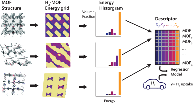
Figure 41: Overall machine learning workflow used by Bucior et al.²⁵⁴ to predict the H2 storage capacity of MOFs. For each MOF, an energy grid within the MOF unit cell was computed, from which an energy histogram was obtained, which is a feature in their regression model that they used to predict the H2 uptake. Figure adopted from Bucior et al.²⁵⁴

Closely related is the use of the heat adsorption as a descriptor in ML models. Similar to the interaction energy captured by the energy histograms, it is a crude estimate of the target. It was for example used in recent studies on adsorption-based heat pumps, where a working fluid is adsorbed by the adsorbent and the released heat is used to drive the heat pump. MOFs are an interesting alternative for the conventional adsorbents.⁴⁷³ The most commonly used working fluid is water but for applications below $0\text{\,}\mathrm{\SIUnitSymbolCelsius}$ one would like to use an alternative fluid.⁴⁷⁴ Shi et al.⁴⁷⁵ used ML to identify that the density and the heat of adsorption are the most important features from their descriptor set (including geometric properties and the maximal working capacity) for models for identifying the optimal MOF for a methanol-based adsorption-driven heat pump. Li et al.⁴⁷⁶ used a similar approach, using the Henry coefficient $K_{\mathrm{H}}$ as a surrogate for the target, to build ML models that identify promising COFs and MOFs for ethanol-based adsorption.

Geometric Descriptors

As we already indicated, most of the works on ML of the adsorption of non-polar gases in porous materials simply trained their models using geometric descriptors.^{477, 478, 419}

Following the idea that MOF databases are likely to contain redundant information, Fernandez et al. performed archetypal analysis (AA) and clustering on geometrical properties to identify the “truly significant” structures.⁴⁷⁹ AA is a matrix decomposition technique that deconstructs the feature matrix, in their case built from geometric properties, into archetypes that do not need to be contained in the data and which can be linearly combined to describe all the data. They trained classifiers on the $20\text{\,}\mathrm{\char 37\relax}$ of structures that are closest to the archetypes and cluster centroids and propose the rules which their DTs learned as rules of thumb for enhancing CO2 and N2 uptake.

Using only geometric descriptors, Thornton et al. developed an iterative prescreening workflow to explore the limits of hydrogen storage in the Nanoporous Materials Genome. After running GCMC simulations on a diverse set of zeolites, they trained a NN on that data and used it to predict a set of 1,000 promising candidates, for which they again ran GCMC simulations and repeated this cycle two more times to reduce the computational time (cf. Figure 42).

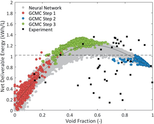
Figure 42: Net deliverable energy as a function of the void fraction for the data predicted using the NN and experimental data. The solid dark line shows the Langmuir model. Figure reproduced from Thornton et al.⁴⁴¹

Using the Building Blocks as Features

In contrast to all aforementioned studies, Borboudakis et al. chose a featurization approach that is not based on geometric properties but that encodes the presence (and absence) of building blocks. In this way, it is not possible for the model, which they trained with an automated ML tool (cf. section 10.1), to perform predictions for structures with building blocks that are not in the training set.¹⁷² This approach was recently generalized by Fanourgakis et al. who use statistics over atom types (e.g., minimum, maximum and average of triple bonded carbon per unit cell), that would usually be used to set up force field topologies, as descriptors to predict the methane adsorption in MOFs.²⁵⁶

Graph-Based Descriptors

Ohno and Mukae used a different set of descriptors, which have also been used with great success in other parts of chemistry. They decided to use molecular graphs to describe the building blocks of the structures (cf. section 4.2.2) and then used a kernel-based technique (Gaussian process regression, cf. section 5.2.3) to measure similarities between the structures.⁴³⁶ They used this kernel in a multiple kernel approach together with pore descriptors and then performed a random search to find the combination of linkers and pore properties that maximizes the prediction (methane uptake) of their model.
Recently, Korolev et al. benchmarked GCNN (cf. section 4.2.2) on different materials classes and also considered the prediction of the bulk and shear modulus of pure-silica zeolites and the Xe/Kr selectivity of MOFs.⁴³⁴ For both applications they found worse performance than with the GBDT baselines which let the authors to conclude that pore-centered descriptors are more suitable for porous materials than atom centered descriptors. Still, GCNN are a promising avenue as the same framework can be applied to many structure classes without tedious feature engineering.

Describing the Pore Shape Using Topological Data Analysis

A different approach for the description of a similarity between pores has been developed by Lee et al. Using topological data analysis, they create persistent homology barcodes (see section 4.2.2). By means of this pore-shape analysis, the authors could find hypothetical zeolites that have similar methane uptake as the top-performing experimental structures.^{238, 237} Lee and co-workers recently also used this descriptor to train machine learning models to predict the methane deliverable capacity of zeolites and MOFs.²³⁴ To do so, they had to derive fixed-length descriptors based on the original persistent homology barcodes which cannot easily be used in ML applications as the number non-zero elements of the barcodes are of varying lengths. They worked around this limitation by using the distances with respect to landmarks, which are a selection of the most diverse structures, as well as some statistics describing the persistent homology barcode (like the mean survival time, the latest birth time). A approach related to the distance to barcodes has been chosen by Moosavi, Xu et al.  who used the distance between barcodes to define a kernel which they then used to train a KRR model for the methane deliverable capacities of porous molecular crystals.¹⁸⁵

Predicting Full Isotherms

The works we described so far were built to predict one specific point on a gas adsorption isotherm (i.e., at one specific temperature and pressure). But in practice, one often wants multiple points on the isotherm, or even the full isotherm, for process development. In principle, one could imagine training one model per pressure point. But we also all know that this is a waste of resources as there are laws that connect the pressure and the loading (e.g., Langmuir adsorption). This motivated researchers to investigate whether one single ML model can be used to predict the full isotherm.

Recently, Sun et al. reported a multitask deep NN (SorbNet) for the prediction of binary adsorption isotherms on zeolites.⁴⁸⁰ Their idea was to use a model architecture in which the two components have two independent branches in the neural network close to the output and share layers close to the inputs, which are the initial loading, the volume, and the temperature. They then used this model to optimize process conditions for desorptive drying, which highlights that such models can help avoid the need for iteratively running simulations for the optimization of process conditions (we discuss the connection between materials simulation and process engineering in more detail in the next section). A limitation of the reported model is that it does not use any descriptors of the sorbate or the porous framework and is therefore limited to a specific combination of sorbates and framework and needs to be retrained for new systems. A recent work by Desgranges uses the same inputs ($N,V,T$, or $N_{1},N_{2},V,T$, respectively) to predict the partition function, which in principle gives them access to all thermodynamic quantities.⁴⁸¹ But similar to the work of Sun et al. the model remains limited to the systems (gas and framework) it was trained on. An interesting avenue might be to combine this approach with the ideas from Anderson et al. who encode the sorbates by training with different achemical species (e.g., varying the Lennard-Jones interaction strength, $\epsilon$).^{482, 483}

Most of the works we discussed so far trained their models on data that were generated with force fields (FFs). But in some cases this is not accurate enough. Correlated method such as RPA might enable simulations to reach chemical accuracy ($1\text{\,}\mathrm{k}\mathrm{c}\mathrm{a}\mathrm{l}\mathrm{/}\mathrm{mol}$). Unfortunately, those methods are prohibitively expensive for use in MD simulations. For this reason, Chehaibou et al. combined several (ML) techniques to predict adsorption energies of CO2 and CH4 in zeolites.⁴³⁸ First, they ran MD simulations with an affordable DFT functional, then they selected a few distant snapshots on which they performed RPA calculations. They used these calculations to train a KRR model for which they used a SOAP kernel to describe the similarity between structures. Interestingly, they also use the $\Delta$-ML approach in which they predict the different between the RPA and DFT energy. This is based on the reasoning that the DFT result already gives the majority of the contribution to the RPA total energy, wherefore it is not necessary to learn this part (cf. section 10.3). Using thermodynamic pertubation theory, they reweighted the DFT trajectory using the RPA energies predicted using the KRR model to get ensemble averages on RPA level.

9.1.3 Bridging the Gap Between Process Engineering and Materials Science

Materials’ design is nearly always a multiobjective optimization in which the goal is to find an optimal spot on the Pareto front of multiple performance metrics. One issue with performance metrics is that it is not always clear how they relate to the actual performance on a process level, e.g. in a pressure swing adsorption system. This is also reflected in the 2018 Mission Innovation report that highlights the need to “understand the relationship between material and process integration to produce optimal capture designs for flexible operation—bridging the gap between process engineering and materials science”.⁴⁸⁴ ML might help to bridge this gap.^{485, 486, 487, 488} Motivated by the need to integrate materials science and process engineering, Burns et al. performed molecular simulations and detailed simulations for a vacuum swing adsorption process for carbon capture on 1632 MOF.⁴⁸⁹ When attempting to build ML models that can predict the process level performance metrics they realized that they can predict the ability of a material to reach the $95\text{\,}\mathrm{\char 37\relax}$ CO2 purity and $90\text{\,}\mathrm{\char 37\relax}$ CO2 recovery targets (95/90-PRT)—but not the parasitic energy, which is the energy needed to recover the sorbent and to compress the CO2. Furthermore, using their RF models they found the N2 adsorption properties to be of the highest importance for the prediction of the 95/90-PRT.

9.1.4 Interpreting the Models

Over the years QSPR has evolved from visual inspection of relationships,⁴⁶⁵ over the use of more and more complex models to the interpretation of these models, e.g., using some feature importance analysis. On the one hand, these analyses can give potentially more insights, also for new materials but, on the other hand, they introduce new error sources. As we discussed in section 8, we not only have to consider the limitations of the dataset for such analyses but also the limitations of the ML model, that might not be able to capture these relationships.

The use of tree-based models,^{490, 491, 477, 492, 476, 475, 493} and the feature importance that can be extracted from them (e.g., based on how high in the tree a feature was used for a split) have evolved to the most popular techniques to interrogate ML models in the MOF community.^{494, 432, 478, 495}

For example, Gülsoy fitted decision trees for the CH4 storage capacity of MOFs using two different feature sets²⁴⁸. Similar trees were also derived by Fernandez and Barnard as “rules of thumb” for CO2 and N2 uptake in MOFs ⁴⁷⁹.

Anderson et al. used feature importance analysis on a library of hypothetical databases for a selection of storage and separation tasks and found that the importance of different features depends on the task. For example, they found chemistry-related metrics (such as the maximum charges) to be more important for CO2/N2 mixtures than for only the uptake of CO2⁴⁹⁵ (see Figure 43). One advantage of ML models is that they can potentially be used for materials’ design, i.e., to design a material with an optimal performance from scratch. Anderson et al. attempted to do so by using a genetic algorithm to find feature combinations that maximize the performance indicators.

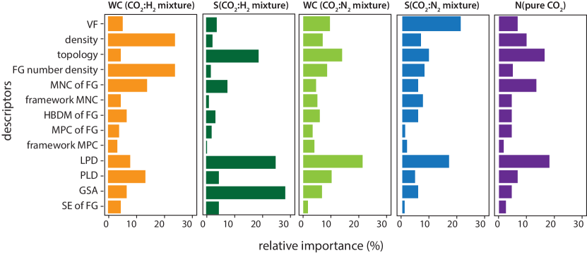
Figure 43: Relative importance of the different material descriptors for carbon capture, as obtained for GBDT models trained by Anderson et al.⁴⁹⁵ In these plots S = selectivity, WC = working capacity, N = adsorption loading. FG = functional group, VF = void fraction, HDBM = highest dipole moment, MPC = most positive charge, MNC = most negative charge, LPD = largest pore diameter, PLD = limiting pore diameter, SE = sum of epsilons, GSA = gravimetric surface area. Figure adopted from Anderson et al.⁴⁹⁵.

9.2 Stability

But also the MOF with the best gas adsorption properties is not of much use if it is not stable. One needs to distinguish between chemical stability and mechanical stability.⁴⁹⁶

The issue of chemical stability is one of the most asked questioned after a MOF presentation. Indeed, MOF-5, one of the first published MOFs, is not stable in water and therefore there is a strong perception that therefore all MOFs have a water issue. However, one has to realize that MOF are, like polymers, a class of materials. Some can be boiled in acids for months without losing their crystallinity while others readily dissolve in water.⁴⁹⁷ For most practical applications it is important, however, to know whether a structure is stable in water. For this reason, there have been efforts to develop models that are able to predict the stability of porous materials based on readily available descriptors. This is a typical example of a less well-defined property as can be seen by the different proxies that are used to mimic the notion of stability. Most of these proxies are based on the idea that for a chemically unstable MOF it is favorable to replace a linker by water. To the best of our knowledge, no ML studies have been reported that investigate the chemical stability. Yet this is a complex topic in which ML might give us some interesting insights.

Sufficient mechanical stability is also of considerable practical importance. In most practical applications MOFs need to be processed, and during this processing there will be pressure and shear forces applied on the crystal. If this causes the pores to deform, the properties of the material may change significantly. Therefore, sufficient mechanical stability is an important practical requirement. Yet, it is not a property that is often studied.^{498, 499, 500}

Evans and Coudert took on this challenge by training a GBDT to predict the bulk and shear moduli based on geometrical properties for 121 training points calculated using DFT.³²⁸ Moghadam et al. followed up this work by training a NN on bulk moduli of more than 3000 MOFs that they obtained from FF-based simulations.⁵⁰¹ Their model uses geometric descriptors and also information about the topology, which their EDA showed to be of utter importance. Recently, the group around Coudert extended their analysis of the mechanical properties of zeolites using FF-derived mechanical properties for all structures from Deem’s database of hypothetical zeolites⁵⁰² for a subset of which they also computed the mechanical properties using DFT. Motivated by the lackluster performance of the FF to describe the mechanical properties, they trained a GBDT (using the same approach which they also used in their first work) on the data derived with DFT. And they found that, on average, their model can predict the Poisson’s ratio better than the FF.

For a related family of porous materials, organic cages, mechanical stability is even a bigger problem as they lack 3D bonding. Turcani et al. built models to predict the stability of the cages based on the precursors to focus more elaborate investigations on materials that are likely mechanically stable.⁵⁰³

Such a tool would certainly also benefit screenings of MOFs, but the lack of good training data makes it difficult to create such a model and also explains the scarcity of the studies in this field. An important part of a solution for this problem is the adoption of standardized computing protocols—such that different databases can be combined into one training set—and sharing of the data in a findable, accessible, interoperable, reusable (FAIR) compliant way.⁵⁰⁴

9.3 Reactivity and Chemical Properties

One of the emerging topics in MOFs is catalysis.^{505, 506, 507, 508} MOFs are interesting for catalysis as the presence of OMS or the specifics of the linker can be combined with concepts of shape selectivity known from zeolite catalysis.⁵⁰⁹

For reactivity on surfaces,⁵¹⁰ but also in zeolites,^{511, 512, 513} scaling relations (that often incorporate the heat of adsorption of the reactants) have been proven to be a powerful tool to predict and rationalize chemical reactivity. Rosen et al. recently introduced such relationships, for example, based on the H-affinity of open metal sites, for methane activation in MOFs.⁵¹⁴ As Andersen et al. recently pointed out, more elaborate MLs techniques like compressed sensing (cf. section 4.3.2) might help us to go beyond scaling relationships and discover hidden patterns in big data. This approach is motivated by the realization that some phenomena might not be describable by a simple equation and that data-driven techniques might be able to approximate those complex relationships.⁵¹⁵

9.4 Electronic Properties

Other emerging applications of MOFs are photocatalysis,⁵¹⁶ luminescence,^{517, 518} and sensing.^{519, 520} For these properties it is important to know the electronic (band) structure. However, ML studies on the electronic properties of MOFs are scarce due to the lack of training data in open databases, and the fact that this data is expensive to create using DFT due to the large unit cells of many MOFs. This motivated He et al. to attempt to use transfer learning.²⁴⁶ They trained four different classifiers on inorganic structures from the open quantum materials database (OQMD) in which the band gaps have been calculated for about 52,300 materials using DFT, and then retrained the model to classify nearly 3,000 materials from the computationally ready experimental (CoRE)-MOF database as either metallic or non-metallic using their ML model.

A key descriptor for the chemistry of materials, that is also needed as input for electronic structure calculations, is the oxidation state of a material. Jablonka et al. retrieved the oxidation states assigned in the chemical names of MOFs in the CSD and trained an ensemble of classifiers to assign the oxidation state,⁴³⁹ using features that, amongst other, describe the geometry of local coordination environments.⁵²¹ Using the ensemble they not only made the model more robust (cf. section 5.2.5) but also obtained an uncertainty measure. In this way, they could not only assign oxidation states with high predictive performance but also find some errors in the underlying training data.

9.5 ML for Molecular Simulations

In other parts of chemical science, HDNNPs received a lot of attention as they promise to create potentials in ab initio quality that can be used to run simulations at a cost of FF based simulation with the additional advantage of the ability to describe reactions (bond breaking and formation). Also, popular molecular simulation codes such as large-scale atomic/molecular massively parallel simulator (LAMMPS) have been extended to perform simulations with such potentials. However, such models are usually trained on DFT reference data which can make it a demanding task to create a training a set given the large unit cells of MOFs.

Figure 44: Molecular basis fragments used by Eckhoff and Behler as starting points for the generation of reference structures for the training of the HDNNP for MOF-5. Based on the five fragments, more than 4,500 other fragments were generated by scaling of the coordinates and small random displacements. All atoms that have complete bulk-like environments within a cutoff radius of $12\text{\,}\mathrm{\SIUnitSymbolAngstrom}$ are shown as balls, capping hydrogen atoms, to saturate broken bonds, are shown in orange. Figure reprinted from Eckhoff and Behler.²⁸⁷

Eckhoff and Behler attempted to avoid this problem by constructing a potential based on more than 4,500 small molecular fragments (the base fragments are shown in Figure 44) that were constructed by cutting out fragments from the crystal structure of MOF-5. The HDNNP which they trained in this way was able to correctly describe the negative thermal expansion and the phonon density of states.²⁸⁷

Besides a potential that describes the interatomic interactions, the assignment of partial charges is needed to calculate the Coulomb contribution to the energy in molecular simulations. The most reliable methods to assign those charges rely on DFT derived electrostatic potentials and in this way can easily become the bottleneck for molecular simulations. As an alternative, Xu and Zhong proposed to use connectivity-based atom types, for which it is assumed that atoms with the same connectivity have the same charge.⁵²² Korolev and co-workers attempted to solve the main limitation of the connectivity-based atom types, namely that all relevant atom types need to be included in the training set, using a ML approach.⁴¹⁷ To do so, they trained a GBDT on 440,000 partial charge assignments using local descriptors such as the electronegativity of the atom or local order parameters, which are based on a Voronoi tessellation of the neighborhood of a given site.

9.6 Synthesis

Synthesis is at the heart of chemistry. Still, it is unfeasible to use computational approaches to predict reactivity or to suggest ideal reaction conditions—also because for example crystallization is a complex interfacial phenomenon that is influenced by structure-directing agents or modifiers.⁵²³ For this reason, chemical reactivity is one of the most promising fields for ML.

Nevertheless, there are only a few reports that try to use artificial intelligence techniques in the synthesis of MOFs. This is likely due to the same reasons as for reactivity and electronic properties, for which there are also no large open databases of properties and for which the training data is expensive to generate.

Some of the early works in the field set out to optimize the synthesis of zeolites. Corma et al. attempted to make high-throughput synthesis (e.g., using robotic systems) more efficient, i.e., improve on classical DoE techniques like full factorial design (generating all possible combinations of experimental parameters, cf. section 3.2.1)^{524, 525} by reducing the number of low-promising experiments.⁵²⁶ First, they attempted to use simple statistical analysis to estimate the importance of different experimental parameters and then moved to actual predictive modeling. After training a NN on synthesis descriptors to predict and optimize crystallinity,^{527, 526} they combined a genetic algorithm (GA) with a NN to guide the next experiments suggested by the GA with the knowledge extracted by the NN ⁵²⁸ (using the NN to predict the fitness).⁵²⁸ A related approach was introduced to the field of MOF synthesis by Moosavi et al. where the synthesis parameters were optimized using a GA. To make this more efficient, the authors introduced the importance of variables derived from a RF model, that was also trained on the failed experiments, as weights for the distance metric for the selection of a diverse set of experimental parameters. In this way, they could synthesize the HKUST-1 with the highest Brunauer–Emmett–Teller (BET) surface area reported so far.²¹

In a similar vein, Xie et al.⁵²⁹ analyzed failed and partly successful experiments and used a GBDT to determine the importance of experimental variables that determine the crystallization of metal-organic nanocapsuless (MONCs), which are compounds that can self-assemble and form porous crystals in some cases.⁵³⁰

Given the large body of experimental procedures for the synthesis of porous materials many works attempted to mine or extract this collective knowledge to create structured datasets that can be used to train ML models for reaction condition prediction.

Figure 45: First four layers of a decision tree for zeolite synthesis that Muraoka et al. extracted from a GBDT model fitted on literature data. The percentages give the fractions of the dominant phases for the complete tree with 12 layers. According to this tree, the most important factor for predicting the synthesis result is the Na/(Si + Al) ratio. Figure reprinted from Muraoka et al.⁵³¹

A recent study of Muraoka et al. was enabled by a literature review on the synthesis of zeolites. Using this data, they trained ML models to predict the phase based on parameters describing the synthetic conditions, producing decision trees, as shown in Figure 45, that reflect chemically reasonable knowledge extraction from the literature data. For example, the authors compare the early split based on the Si/Al ratio with Löwenstein’s rule that forbids Al-O-Al bonds. By optimizing the structural fingerprint by re-weighting the similarity between zeolites to be similar in the synthesis and structure space, they could build a similarity network in which they could uncover an overlooked similarity between zeolites that also manifested itself in the synthesis conditions.⁵³¹

Jensen et al. developed algorithms to retrieve the synthesis conditions from 70,000 zeolite papers and used this to build a model that can predict the framework density of germanium zeolites based on the synthetic conditions.⁵³² Also, Schwalbe-Koda mined the literature about polymorphic transformations between zeolites to enable their work in which they showed that graph isomorphism can be used as a metric for these transformations.⁵³³

For MOFs, Park et al.¹⁵⁸, as well as Tayfuroglu et al.⁵³⁴, parsed the literature to retrieve surface areas and pore volumes for a large collection of MOF. But so far, the data generated from these studies have not yet been used to build predictive models for MOF properties and synthesis.

Another approach was taken by Deem and co-workers who addressed the design of organic structure directing agents (OSDAs).⁵³⁵ Zeolites are all isomorphic structures and OSDAs are used during the synthesis to favor the formation of the desired isomorph. Finding the right OSDA to synthesize a particular zeolite is seen as one of the bottlenecks. To support this effort, Deem and co-workers developed a materials’ design program to generate synthetically accessible OSDA.⁵⁰² To expedite this process, Deem and co-workers developed a ML approach, in which they calculated the stabilization energy of different OSDAs inside of zeolite beta and then trained a NN using molecular descriptors derived from ideas of electron diffraction.⁵³⁶ In this way, they could speed up the search for novel OSDA by a factor of 350 and suggest 469 new and promising OSDA (see Figure 46). Daeyaert and Deem⁵³⁷ further extended this work to find an OSDA for some of the hypothetical zeolites that were found to perform optimally in a screening study for the separation of CO2 and CH4.⁴⁶²

Figure 46: Deem and co-workers used a ML approach to identify chemically synthesizable OSDA for zeolite beta, which is one of the top-six zeolites of commercial interest. The figure shows the top-three OSDAs that Deem and co-workers discovered.⁵³⁵ The scores in the figure are the binding energy in kJ/(mol Si). Figure adopted from ref.⁵³⁵

Even if one manages to create some material it is not always trivial what the material is. To address this, Wang et al. build models, including CNNs similar to the one we described in section 5.1.1 to identify the material based on its experimental XRPD pattern. To do so, they predicted diffraction patterns for structures deposited in the CSD and used data augmentation techniques (cf. section 3.4) like the addition of noise and then tested their model using experimental diffraction patterns.¹³⁵

9.6.1 Synthesizability

One question that always arises in the context of hypothetical materials is the question of synthesizability. In the context of zeolites, this question received a lot of attention. Early works proposed that low framework energies are the distinctive criterion^{538, 539, 540}—akin to the recent attempt of Anderson and Gómez-Gualdrón to assess the synthetic feasibility of MOFs.⁵⁴¹ But this quickly got overturned with the discovery of high-energy zeolites and replaced by a “flexibility window”,⁵⁴² which was eventually also found to not be reliable and replaced by criteria that focus on local interatomic distances.⁵⁴³ A library of such criteria was used in a screening study of Perez et al. to reduce the pool of candidate materials from over 300,000 to below 100. As a conclusion of their study, they suggest using the overlap between the distribution of descriptors of experimental materials and those generated in silico as a metric to evaluate how feasible the materials are which an algorithm produces.⁵⁴⁴ Such an approach, which is related to approaches suggested for benchmarking of generative techniques for small molecules,^{545, 546} might also be useful for evaluation of the generative models that we discuss in the following.

9.7 Generative Models

The ultimate goal of materials’ design is to build a model that, given desired (application) properties, can produce candidate structures using generative techniques like GANs. Though this flavor of ML is formally not supervised learning, on which we focused in this review, we give a short overview of recent progress in this promising application of ML to porous materials. One model architecture that is often used in this context are GANs where a first NN acts as generator and tries to “deceive” a discriminator NN that tries to distinguish real data (structures) from the “fake” ones that the generator generated. For molecules, this approach received wide attention,^{64, 24} but the works on nanoporous solids proved to be more difficult due to the periodicity and the non-unique representation of the unit cell. Kim and co-workers started building GANs that can generate energy grids of zeolites⁵⁴⁷ and recently extended their model to predict the structure of all-silica zeolites.⁴³⁵

Figure 47: Distribution of Henry coefficient, void fraction and heat of adsorption for generated structures with a user-defined target range of $18\text{\,}\mathrm{kJ}\text{\,}{\mathrm{mol}}^{-1}22\text{\,}\mathrm{kJ}\text{\,}{\mathrm{mol}}^{-1}$ for the heat of adsorption. Reproduced from ref. ⁴³⁵.

To do so, they used a separate channel (as it is used for the RGB channels in color images) for oxygen and silicon atom positions which they encoded by placing Gaussian at the atom positions. By adjusting the loss function to target structures with a specific heat of adsorption, they could observe a drastic shift in the shape of the distribution of this property but not in the one for the void fraction or the Henry coefficient.

10 Outlook and Concluding Remarks

One of the aims of this review is to provide a comprehensive overview of the state of the art of ML in the field of materials science. In our review, we not only discuss the technical details, but we also try to point out the potential caveats that are more specific for material science. As part of the outlook, we discuss some techniques that are, as of yet, little, if at all, used for porous materials. Yet, these methods can address some of the issues that we have discussed in the previous sections.

10.1 Automatizing the Machine Learning Workflow

Given that the complete process from structure to prediction, which we discussed in this review, is quite laborious, there is a significant barrier for scientists with little computational background to enter the field. To lower the entrance barrier, a lot of effort is spent to automatize the ML process.⁵⁴⁸ In the ML community tools like H2O’s autoML,⁵⁴⁹ TPOPT⁵⁵⁰ or Google’s AutoML are widely known and receive mounting attention.⁵⁵¹ In the materials science community especially the chemml^{552, 553} and the automatminer package⁵⁵⁴ are worth mentioning. Latter uses matminer to calculate descriptors that are relevant for materials science, performs the feature selection (using TPOPT) as well as training and cross-validation.⁵⁵⁴ Such tools will lower the barrier for domain experts even more and also help practitioners of ML to expedite tedious tasks.

10.2 Reproducibility in Machine Learning

Reproducibility, and being able to build on top of previous results, is one of the hallmarks of science. And it is also one of the main technical debts of ML systems, where technical debt describes costs due to (code) rework that are caused by choosing an easy solution now instead of a proper one that might take longer to be developed.⁵⁵⁵ If one cannot even replicate published experiments one can ask if we are making any progress as a community. This question was posed by a recent study that found that they could only reproduce 7 from 18 recommender algorithms. Moreover, six of the algorithms which were reproducible could be outperformed by simple heuristics.⁵⁵⁶

It is also the authors’ personal experience that reproducing computational data from the literature can be a painful process. Even, if the literature is an article from the same group, reproducing the results from only a few years earlier can be a difficult search for the information that was not reported in the original article. Often, the reason for being unable to reproduce the data is that many programs use default settings. These default settings can be hidden in the input files—or in the code itself—and since they are never changed during the reported studies, these settings get overlooked and do not get reported. However, if in a new release or for any other reasons the defaults get changed, the results become nearly impossible to reproduce. Of course, if we had realized the importance of these unknown unknowns, we, and any other author, would have reported the values in the original article. The only way to avoid these issues is to rigorously report all input and output files as well as workflows for all computations.⁵⁵⁷ In ML the same holds—for example different implementations of performance measures (e.g., in off-the-shelf ML libraries) can lead to different, biased, estimates that hinder comparability and reproducibility.⁵⁵⁸

In computational materials science there are ongoing efforts, like the AiiDA infrastructure⁵⁵⁹ or the Fireworks workflow management system,⁵⁶⁰ to make computational workflows more reproducible and to lower the barrier of applying the FAIR principles of data sharing.⁵⁶¹ For example, Ongari et al.⁵⁶² developed a workflow to optimize and screen experimental COFs structures for their potential for carbon capture.⁵⁶²

Figure 48: Screenshot of the Materials Cloud (https://archive.materialscloud.org/2019.0034/v2) pages for the screening of COFs for carbon capture. In the “Discover” section (a) there is an interactive plot and table that links to the original references and structures as well as to plots of the relaxation and the process optimization which are all linked to the “Explore” section (b), where one can find the source code for the workflows and interactive provenance graphs.

Figure 48 shows a snapshot from the Materials Cloud website where, by clicking on a data point, one not only obtains all data that have been computed for this particular material, but also the complete provenance. This provenance includes an optimization step of the experimental structure, the computation of the charges on the framework, the GCMC simulations to compute the isotherms and heats of adsorption, and finally the program that computes the objective function used to rank the materials for carbon capture. The idea here is that anybody in the world can reproduce the data by simply downloading the AiiDA scripts and running the programs on a local computer. Or, by adding more structures, extending to work to other materials, or reproducing the complete study using a different force field, by simply replacing the force field input file. Given that the data contains rich metadata, and all parameters of the calculations, it is easy to identify with which other databases it could be combined to create a training set for a ML algorithm.

But these workflow management tools, and even version control system like git, are not easily applicable to ML problems, where one usually wants to share and curate data separately from the code, but still retain the link between data, hyperparameters, code, and metrics. Tools like comet,⁵⁶³ neptune,⁵⁶⁴ provenance,⁵⁶⁵, Renku,⁵⁶⁶ mlflow,⁵⁶⁷ ModelDB,⁵⁶⁸ and dvc⁵⁶⁹ try to make ML more reproducible by providing parts of this solution, like data version control or automatic tracking of hyperparameter and metrics together with data hashes.

We consider both reproducibility and sharing of data as essential for the progress in this field. Therefore, to promote the adaptation of good practices, we encourage using tools such as the data-science cookiecutter⁵⁷⁰ that automatically sets up a ML development environment that promotes good development practices.

Journals in the chemical domain might also encourage good practices by providing “reproducibility checklists”, similar to the major ML conferences like NeurIPS.⁵⁷¹

Publishing the full provenance of the model development process, as it can be done for example with tools like comet, can to some extent also remedy the problem that negative results (e.g., plausible architectures that do not work) are usually not reported.

10.2.1 Comparability and Reporting Standards

One factor that makes it difficult to build on top of previous work is the lack of standardization. In the MOF community, many researchers use hypothetical databases to build their models. But unfortunately, they typically use different databases, or different train/test splits of the same database. This makes it difficult to compare different works as the chemistry in some databases might be less diverse and easier to learn than for example in the CoRE-MOF database, which contains experimental structures. Also, in comparing the protocols with which the various labels ($y$) for different databases are created, one often finds worrying differences, e.g., in the details of the truncation of the interaction potential⁵⁷² or the choice of the method for assigning partial charges. This can make it necessary to recompute some of the data, as the discrepancy between the two approaches will dictate the Bayes basis error.^{280, 215} Unfortunately, there are no widely accepted benchmark sets in the porous materials community—even though the ML efforts on (small) molecules greatly benefited from such benchmark sets (see e.g. http://quantum-machine.org/datasets/ or MoleculeNet³⁶⁷) which allow for a fair comparison between studies.⁴²⁸ We are currently working on assembling such sets for ML studies on porous materials.

In addition to the lack of benchmark sets, there is also a lack of common reporting standards. Not all works provide full access to data, features, code, trained models, and choice of hyperparameters—even though this would be needed to ensure replicability. The crystals.ai project is an effort to create a repository for such data.⁵⁷³ Again, reproducibility checklists, like the one for NeurIPS, might be beneficial for our community to ensure that researchers stick to some common reporting standard.

10.3 Transfer Learning and Multifidelity Optimization

A problem of ML for materials science, and in particular MOFs with their large unit cells, is that the datasets of the ground truth (the experimental results) are scarce and only available for a few materials. Often, experimental data are replaced by estimates from computations, and these computational data necessarily introduce errors due to approximations in the theories.¹⁴² Similarly, it is much easier to create large datasets using DFT than using expensive, but more accurate, wavefunction methods. But even DFT can still be prohibitively expensive for large libraries of materials with large unit cells. This is why multifidelity optimization (which combines low and high-fidelity data, like semi-empirical and DFT-level data) and transfer learning are promising avenues for materials science.

Transfer learning has found widespread use in the “mainstream” ML community, e.g., for image recognition, where models are trained on abundant data and then partially (re)-trained on the less abundant (and more expensive) data. Hutchinson et al. used transfer learning techniques to predict experimental band gaps and activation energies using DFT labels as the main data source and showed that transfer learning generally seems to be able to improve predictive performance.¹⁴² Related to this is a recent physics-based neural network from the Pande group in which a cheap electron density, for example from Hartree-Fock (HF), is used to predict the energetics and electron density on the “gold standard” level of theory (Coupled Cluster Single-double with pertubative triple excitations (CCSD(T))).⁵⁷⁴ The authors relate the expensive electron density $\rho$ to the cheap one using a Taylor expansion and use a CNN to learn the $\Delta\rho$ and $\Delta E$. Since both Taylor expansions for $\Delta E$ and $\Delta\rho$ share terms like $\left(\frac{\delta^{2}E}{\delta\rho(\mathbf{r})\delta\rho(\mathbf{r}^{\prime})}\right)$ they can use the same first layers and then branch into two separate output channels for $\Delta\rho$ and $\Delta E$, respectively. The NN was first trained using less expensive DFT data, and then transfer learning was used to refine the weights using the more expensive and less abundant CCSD(T) densities. This is similar to the approach which was used to bring the ANI-1 potential to CCSD(T) accuracy on many benchmark sets.²⁸⁸

But for transfer learning to find more widespread use in the materials science domain it would be necessary to share the trained models, and the training as well as evaluation data, in an interoperable way.

The fact that inaccurate, but inexpensive, simulation data is widely available motivated the development of the $\Delta$-ML technique, where the objective of the ML model is to predict the difference between the result of a cheap calculation and one obtained at a higher level of theory.³⁶ This approach was subsequently formalized and extended in multiple dimensions using the sparse grid combination technique, which combines models trained on different subspaces (e.g. combination of basis set size and correlation level) such that only a few samples are needed on the highest, target, level of accuracy.⁵⁷⁵

A different multifidelity learning approach, known as co-kriging, can combine low- and high-fidelity training data to predict properties at the highest fidelity level—without using the low-fidelity data as features or baseline. This technique was used by Pilania et al. to predict band gaps of elpasolites on hybrid functional level of theory using a training set of properties on both GGA and hybrid functional level.³⁰⁴

All these methods are promising avenues for ML for porous materials.

10.4 Multitask Prediction

In the search for new materials, we usually do not only to want to optimize one property but multiple. Also, we usually not only have training data for only one target but also for related targets, e.g., for Xe, Kr and CH4 adsorption. Multitask models are built around this insight and that models, particularly NNs, might learn similar high-level representations to predict related properties (e.g., one might expect the gas uptake for noble gases and CH4 follow the same basic relationship). Hence, training a model to predict several properties at the same time might improve its generalization performance due to the implicit information captured between the different targets. In the chemical sciences, Zubatyuk et al. used multimodal training to create an information-rich representation using a message-passing NN.¹⁴¹ This representation could then be used to efficiently (with less training data) learn new properties. Similar benefits of multitask learning were also observed in models trying to predict properties relevant for drug discovery.^{576, 140}

10.5 The Future of Big-Data Science in Porous Materials

It is tempting to conclude that MOFs and related porous material are synthesized for ML. MOFs are among the most studied materials in chemistry and the number of MOFs that are being synthesized is still growing. In addition, the number of possible applications of these materials is also increasing. We are already in a situation that if a group has synthesized a novel MOF it is in practice impossible to test this novel material for all possible applications. One can then clearly envision the role of ML. If we can capture the different computational screening studies using ML, we should be able to indicate the potential performance of a novel material for a range of different applications. Clearly, a lot of work needs to be done to reach this aim; with this review we intended to show that the foundations for such an approach are being built.

The other important domain where we expect significant progress is in the field of MOF synthesis. The global trend in science is to share more data, and technology makes it easier to share large amounts of data. But the common practice to only publish successful synthesis routes is throwing away lots of valuable information. For example, an essential step in MOF synthesis is finding the right conditions for the material to crystallize. At present, this is mainly trial and error. Moosavi et al.²¹ have shown how to learn from the failed and partially successful experiments. Interestingly, they used as example HKUST-1, which is one of the most synthesized MOFs, but they had to reproduce the failed experiments to be able to analyze the data using ML techniques. One can only dream about the potential of such studies if all synthetic MOF groups would share their failed and partially successful experiments. This would open the possibility to use ML to find correlations between linker/metal nodes and crystallization conditions, and would allow us to make predictions of the optimal synthesis conditions for novel MOFs. Also here, ML methods have the potential to change the way we do chemistry, but the challenges are enormous in solving the practical issues in creating an infrastructure and change of mind set that all synthesis attempts are shared in such a way that the data are publicly accessible.

Hence, a key factor in the success of ML in the field of MOFs will be the extent in which the community is willing and able to share data. If all data on these hundreds of thousands porous materials are shared, it will open up possibilities that go beyond the conventional ways of doing science. We hope that the examples of ML applied to MOFs we discussed in this review, illustrate how ML can change the way we do and think science.

Glossary

Acronyms

AA

archetypal analysis

ADASYN

adaptive synthetic oversampling

AP

atomic property

AUC

area under the curve

BAML

bond-angles machine learning

BET

Brunauer–Emmett–Teller

BoB

bag of bonds

CADD

computer aided drug design

CART

classification and regression tree

CAS

chemical abstract services

CCSD(T)

Coupled Cluster Single-double with pertubative triple excitations

CNN

convolutional neural network

COF

covalent organic framework

CoRE

computationally ready experimental

CSD

Cambridge Structure Database

DFT

density-functional theory

DL

deep learning

DNN

deep neural networks

DoE

design of experiment

DOS

density of states

DT

decision tree

DTNN

deep tensor neural network

EDA

exploratory data analysis

FAIR

findable, accessible, interoperable, reusable

FF

force field

FPS

farthest point sampling

GA

genetic algorithm

GAM

generalized additive model

GAN

generative adverserial network

GAP

Gaussian approximation potential

GBDT

gradient boosted decision trees

GCMC

grand-canonical Monte Carlo

GCNN

graph-convolutional

GGA

general-gradient approximation

GP

Gaussian process

GPR

Gaussian process regression

HDNNP

high-dimensional neural network potential

HF

Hartree-Fock

HIP

hierarchically interacting particle

i.i.d

independently and identically distributed

KMM

kernel-mean matching

$k$NN

$k$ nearest neighbor

KRR

kernel ridge regression

LAMMPS

large-scale atomic/molecular massively parallel simulator

Lasso

least absolute shrinkage and selection operator

LHS

latin hypercube sampling

lococv

leave-on-cluster-out cross-validation

LOOB

leave-one-out bootstrap

LOOCV

leave-one-out cross validation

MAE

mean absolute error

MBTR

many-body tensor representation

MC

Monte-Carlo

MD

molecular dynamics

MDP

maximum diversity problem

ML

machine learning

MLP

multilayer perceptron

MOF

metal-organic framework

MONC

metal-organic nanocapsules

MSE

mean squared error

NLP

natural language processing

NN

neural network

NP

non-deterministic polynomial-time

OBD

optimal brain damage

OMS

open metal site

OQMD

open quantum materials database

OSDA

organic structure directing agent

PCA

principal component analysis

PES

potential energy surface

PLMF

property labeled materials fragments

PPN

porous polymer network

PSD

pore size distribution

QSAR

quantitative structure activity relationship

QSPR

quantitative structure property relationship

RAC

revised autocorrelation

RDF

radial distribution function

REACH

registration evaluation and authorization of chemicals

ReLU

rectified linear unit

RF

random forest

RFA

recursive feature addition

RFE

recursive feature elimination

RMSE

root mean squared error (MSE)

RNN

recurrent neural network

ROC

receiver-operating characteristic

RPA

random phase approximation

SGD

stochastic gradient descent

SHAP

SHapley Additive exPlanations

si

sure independence

SISSO

sure independence screening and sparsifying operator

SMBO

sequential model-based optimization

SMILES

simplified molecular input line entry system

SMOTE

synthetic minority oversampling technique

SOAP

smooth overlap of atomic positions

SVC

support vector classifier

SVM

support vector machine

TDA

topological data analysis

TPE

tree-Parzen estimator

t-SNE

t-distributed stochastic neighbor embedding

VAE

variational autoencoders

VIF

variance inflation factor

XRD

x-ray diffraction

XRPD

x-ray powder diffraction

ZIF

zeolitic imidazolate framework

Author Information

Corresponding author

Berend Smit; e-mail berend.smit@epfl.ch.

Biographies

Kevin Maik Jablonka

received his undergraduate degree in chemistry from the Technical University of Munich and then joined EPFL for his graduate studies, supported by the Alfred Werner fund, during which he also obtained a degree in data science. Currently, he is a PhD student in Berend Smit’s group, investigating the use of data-driven methods for the design and discovery of new materials for energy-related applications.

Daniele Ongari

received his diploma in chemical engineering from Politecnico di Milano. In 2019, he completed his PhD under the supervision of Prof. Berend Smit. His research focuses on the investigation of microporous materials, in particular MOFs and COFs, using computational methods to assess their performances for molecular adsorption and catalysis.

Seyed Mohamad Moosavi

was born in Boroujerd, Iran. He received his undergraduate degree in mechanical engineering from Sharif University of Technology in Tehran, Iran. He has recently defended his PhD in chemistry and chemical engineering at EPFL under the supervision of Prof. Berend Smit. He visited Prof. Kulik’s group at MIT on an SNSF fellowship award. His research interests focus on computational and data-driven design and engineering of novel materials for energy-related applications.

Berend Smit

received a MSc in Chemical Engineering in 1987 and a MSc in Physics both from the Technical University in Delft (the Netherlands). In 1990, he received a cum laude PhD in Chemistry from Utrecht University (the Netherlands). He was a (senior) Research Physicists at Shell Research before he joined the University of Amsterdam (the Netherlands) as Professor of Computational Chemistry. In 2004, he was elected Director of the European Center of Atomic and Molecular Computations (CECAM) Lyon France. Since 2007 he is Professor of Chemical Engineering and Chemistry at U.C. Berkeley and Faculty Chemist at Materials Sciences Division, Lawrence Berkeley National Laboratory. Since July 2014 he is full professor at EPFL.

Berend Smit’s research focuses on the application and development of novel molecular simulation techniques, with emphasis on energy-related applications. Together with Daan Frenkel he wrote the textbook Understanding Molecular Simulations and together with Jeff Reimer, Curt Oldenburg, and Ian Bourg the textbook Introduction to Carbon Capture and Sequestration.

References

- Furukawa et al. 2013 Furukawa, H.; Cordova, K. E.; O’Keeffe, M.; Yaghi, O. M. The Chemistry and Applications of Metal-Organic Frameworks. Science 2013, 341, 1230444
- Chung et al. 2014 Chung, Y. G.; Camp, J.; Haranczyk, M.; Sikora, B. J.; Bury, W.; Krungleviciute, V.; Yildirim, T.; Farha, O. K.; Sholl, D. S.; Snurr, R. Q. Computation-Ready, Experimental Metal–Organic Frameworks: A Tool To Enable High-Throughput Screening of Nanoporous Crystals. Chem. Mater. 2014, 26, 6185–6192
- Chung et al. 2019 Chung, Y. G. et al. Advances, Updates, and Analytics for the Computation-Ready, Experimental Metal–Organic Framework Database: CoRE MOF 2019. J. Chem. Eng. Data 2019, 64, 5985–5998
- Moghadam et al. 2017 Moghadam, P. Z.; Li, A.; Wiggin, S. B.; Tao, A.; Maloney, A. G. P.; Wood, P. A.; Ward, S. C.; Fairen-Jimenez, D. Development of a Cambridge Structural Database Subset: A Collection of Metal–Organic Frameworks for Past, Present, and Future. Chem. Mater. 2017, 29, 2618–2625
- Boyd et al. 2017 Boyd, P. G.; Lee, Y.; Smit, B. Computational Development of the Nanoporous Materials Genome. Nat. Rev. Mater. 2017, 2, 17037
- Halevy et al. 2009 Halevy, A.; Norvig, P.; Pereira, F. The Unreasonable Effectiveness of Data. IEEE Intell. Syst. 2009, 24, 8–12
- Mehta et al. 2019 Mehta, P.; Bukov, M.; Wang, C.-H.; Day, A. G. R.; Richardson, C.; Fisher, C. K.; Schwab, D. J. A High-Bias, Low-Variance Introduction to Machine Learning for Physicists. Phys. Rep. 2019, 810, 1–124
- Butler et al. 2018 Butler, K. T.; Davies, D. W.; Cartwright, H.; Isayev, O.; Walsh, A. Machine Learning for Molecular and Materials Science. Nature 2018, 559, 547–555
- Samuel 2000 Samuel, A. L. Some Studies in Machine Learning Using the Game of Checkers. IBM J. Res. Dev. 2000, 44, 206–226
- Hutson 2019 Hutson, M. Bringing Machine Learning to the Masses. Science 2019, 365, 416–417
- Gray and Szalay 2007 Gray, J.; Szalay, A. eScience-A Transformed Scientific Method, Presentation to the Computer Science and Technology Board of the National Research Council. 2007; https://www.slideshare.net/dullhunk/escience-a-transformed-scientific-method (accessed Nov 11, 2019)
- Hey 2009 Hey, A. J. G., Ed. The Fourth Paradigm: Data-Intensive Scientific Discovery; Microsoft Research: Redmond, Washington, 2009
- Boyd et al. 2019 Boyd, P. G. et al. Data-driven design of metal–organic frameworks for wet flue gas \ceCO2 capture. Nature 2019, 576, 253–256
- Curtarolo et al. 2013 Curtarolo, S.; Hart, G. L. W.; Nardelli, M. B.; Mingo, N.; Sanvito, S.; Levy, O. The High-Throughput Highway to Computational Materials Design. Nat. Mater. 2013, 12, 191–201
- Lin et al. 2012 Lin, L.-C. et al. In Silico Screening of Carbon-Capture Materials. Nat. Mater. 2012, 11, 633–641
- Pyzer-Knapp et al. 2015 Pyzer-Knapp, E. O.; Li, K.; Aspuru-Guzik, A. Learning from the Harvard Clean Energy Project: The Use of Neural Networks to Accelerate Materials Discovery. Adv. Funct. Mater. 2015, 25, 6495–6502
- Curtarolo et al. 2003 Curtarolo, S.; Morgan, D.; Persson, K.; Rodgers, J.; Ceder, G. Predicting Crystal Structures with Data Mining of Quantum Calculations. Phys. Rev. Lett. 2003, 91, 135503
- Collins et al. 2016 Collins, S. P.; Daff, T. D.; Piotrkowski, S. S.; Woo, T. K. Materials Design by Evolutionary Optimization of Functional Groups in Metal-Organic Frameworks. Sci. Adv. 2016, 2, e1600954
- Duan et al. 2019 Duan, C.; Janet, J. P.; Liu, F.; Nandy, A.; Kulik, H. J. Learning from Failure: Predicting Electronic Structure Calculation Outcomes with Machine Learning Models. J. Chem. Theory Comput. 2019, 15, 2331–2345
- Heinen et al. 2020 Heinen, S.; Schwilk, M.; von Rudorff, G. F.; von Lilienfeld, O. A. Machine Learning the Computational Cost of Quantum Chemistry. Mach. Learn.: Sci. Technol. 2020, 1, 025002
- Moosavi et al. 2019 Moosavi, S. M.; Chidambaram, A.; Talirz, L.; Haranczyk, M.; Stylianou, K. C.; Smit, B. Capturing Chemical Intuition in Synthesis of Metal-Organic Frameworks. Nat. Commun. 2019, 10, 539
- Aspuru-Guzik et al. 2018 Aspuru-Guzik, A.; Lindh, R.; Reiher, M. The Matter Simulation (R)Evolution. ACS Cent. Sci. 2018, 4, 144–152
- De Luna et al. 2017 De Luna, P.; Wei, J.; Bengio, Y.; Aspuru-Guzik, A.; Sargent, E. Use Machine Learning to Find Energy Materials. Nature 2017, 552, 23–27
- Sanchez-Lengeling and Aspuru-Guzik 2018 Sanchez-Lengeling, B.; Aspuru-Guzik, A. Inverse Molecular Design Using Machine Learning: Generative Models for Matter Engineering. Science 2018, 361, 360–365
- Pauling 1929 Pauling, L. The Principles Determining the Structure of Complex Ionic Crystals. J. Am. Chem. Soc. 1929, 51, 1010–1026
- Pettifor 1995 Pettifor, D. G. Bonding and Structure of Molecules and Solids; Clarendon Press ; Oxford University Press: Oxford : New York, 1995
- Tukey 1977 Tukey, J. W. Exploratory Data Analysis; Addison-Wesley Series in Behavioral Science; Addison-Wesley Pub. Co: Reading, Mass, 1977
- Lake et al. 2016 Lake, B. M.; Ullman, T. D.; Tenenbaum, J. B.; Gershman, S. J. Building machines that learn and think like people. Behav. Brain Sci. 2016, 40
- Rudin 2019 Rudin, C. Stop Explaining Black Box Machine Learning Models for High Stakes Decisions and Use Interpretable Models Instead. Nat. Mach. Intell. 2019, 1, 206–215
- Schmidt et al. 2019 Schmidt, J.; Marques, M. R. G.; Botti, S.; Marques, M. A. L. Recent Advances and Applications of Machine Learning in Solid-State Materials Science. npj Comput. Mater. 2019, 5, 83
- Tibshirani et al. 2017 Tibshirani, T.; Friedman, J.; Tibshirani, R. The Elements of Statistical Learning - Data Mining, Inference, and Prediction, 2nd ed.; Springer Series in Statistics; Springer, 2017
- Shalev-Shwartz and Ben-David 2014 Shalev-Shwartz, S.; Ben-David, S. Understanding Machine Learning: From Theory to Algorithms; Cambridge University Press: Cambridge, 2014
- Bishop 2006 Bishop, C. M. Pattern Recognition and Machine Learning; Information Science and Statistics; Springer: New York, 2006
- Géron 2019 Géron, A. Hands-on Machine Learning with Scikit-Learn, Keras, and TensorFlow: Concepts, Tools, and Techniques to Build Intelligent Systems; O’Reilly Media, Inc: Sebastopol, CA, 2019
- Raschka et al. 2020 Raschka, S.; Patterson, J.; Nolet, C. Machine Learning in Python: Main Developments and Technology Trends in Data Science, Machine Learning, and Artificial Intelligence. Information 2020, 11, 193
- Ramakrishnan et al. 2015 Ramakrishnan, R.; Dral, P. O.; Rupp, M.; von Lilienfeld, O. A. Big Data Meets Quantum Chemistry Approximations: The -Machine Learning Approach. J. Chem. Theory Comput. 2015, 11, 2087–2096
- Häse et al. 2019 Häse, F.; Roch, L. M.; Aspuru-Guzik, A. Next-Generation Experimentation with Self-Driving Laboratories. Trends Chem. 2019, 1, 282–291
- MacLeod et al. 2019 MacLeod, B. P. et al. Self-Driving Laboratory for Accelerated Discovery of Thin-Film Materials. arXiv:1906.05398 [cond-mat, physics:physics] 2019,
- Häse et al. 2018 Häse, F.; Roch, L. M.; Aspuru-Guzik, A. Chimera: Enabling Hierarchy Based Multi-Objective Optimization for Self-Driving Laboratories. Chem. Sci. 2018, 9, 7642–7655
- Tabor et al. 2018 Tabor, D. P. et al. Accelerating the Discovery of Materials for Clean Energy in the Era of Smart Automation. Nat. Rev. Mater. 2018, 3, 5–20
- Gromski et al. 2019 Gromski, P. S.; Henson, A. B.; Granda, J. M.; Cronin, L. How to Explore Chemical Space Using Algorithms and Automation. Nat. Rev. Chem. 2019, 3, 119–128
- Gromski et al. 2019 Gromski, P. S.; Granda, J. M.; Cronin, L. Universal Chemical Synthesis and Discovery with ‘The Chemputer’. Trends Chem. 2019, 2, 4–12
- Keenan et al. 2019 Keenan, G.; Salley, D.; Martin, S.; Grizou, J.; Sharma, A.; Cronin, L. A Nanomaterials Discovery Robot for the Darwinian Evolution of Shape Programmable Gold Nanoparticles. ChemRxiv preprint 2019,
- Dragone et al. 2017 Dragone, V.; Sans, V.; Henson, A. B.; Granda, J. M.; Cronin, L. An Autonomous Organic Reaction Search Engine for Chemical Reactivity. Nat. Commun. 2017, 8, 15733
- Gasparotto et al. 2018 Gasparotto, P.; Meißner, R. H.; Ceriotti, M. Recognizing Local and Global Structural Motifs at the Atomic Scale. J. Chem. Theory Comput. 2018, 14, 486–498
- Das et al. 2006 Das, P.; Moll, M.; Stamati, H.; Kavraki, L. E.; Clementi, C. Low-Dimensional, Free-Energy Landscapes of Protein-Folding Reactions by Nonlinear Dimensionality Reduction. Proc. Natl. Acad. Sci. U.S.A. 2006, 103, 9885–9890
- Xie et al. 2019 Xie, T.; France-Lanord, A.; Wang, Y.; Shao-Horn, Y.; Grossman, J. C. Graph Dynamical Networks for Unsupervised Learning of Atomic Scale Dynamics in Materials. Nat. Commun. 2019, 10, 2667
- Tribello et al. 2012 Tribello, G. A.; Ceriotti, M.; Parrinello, M. Using Sketch-Map Coordinates to Analyze and Bias Molecular Dynamics Simulations. Proc. Natl. Acad. Sci. U.S.A. 2012, 109, 5196–5201
- Hashemian et al. 2013 Hashemian, B.; Millán, D.; Arroyo, M. Modeling and Enhanced Sampling of Molecular Systems with Smooth and Nonlinear Data-Driven Collective Variables. J. Chem. Phys. 2013, 139, 214101
- Kohonen 1997 Kohonen, T. Exploration of Very Large Databases by Self-Organizing Maps. Proceedings of International Conference on Neural Networks (ICNN’97). 1997; pp PL1–PL6 vol.1
- Beckonert et al. 2003 Beckonert, O.; Monnerjahn, J.; Bonk, U.; Leibfritz, D. Visualizing Metabolic Changes in Breast-Cancer Tissue Using 1H-NMR Spectroscopy and Self-Organizing Maps. NMR Biomed. 2003, 16, 1–11
- Fritzke 1994 Fritzke, B. Growing Cell Structures—A Self-Organizing Network for Unsupervised and Supervised Learning. Neural Netw. 1994, 7, 1441–1460
- Ceriotti et al. 2013 Ceriotti, M.; Tribello, G. A.; Parrinello, M. Demonstrating the Transferability and the Descriptive Power of Sketch-Map. J. Chem. Theory Comput. 2013, 9, 1521–1532
- De et al. 2016 De, S.; Bartók, A. P.; Csányi, G.; Ceriotti, M. Comparing Molecules and Solids across Structural and Alchemical Space. Phys. Chem. Chem. Phys. 2016, 18, 13754–13769
- Isayev et al. 2015 Isayev, O.; Fourches, D.; Muratov, E. N.; Oses, C.; Rasch, K.; Tropsha, A.; Curtarolo, S. Materials Cartography: Representing and Mining Materials Space Using Structural and Electronic Fingerprints. Chem. Mater. 2015, 27, 735–743
- Kunkel et al. 2019 Kunkel, C.; Schober, C.; Oberhofer, H.; Reuter, K. Knowledge Discovery through Chemical Space Networks: The Case of Organic Electronics. J. Mol. Model. 2019, 25, 87
- Samudrala et al. 2013 Samudrala, S.; Rajan, K.; Ganapathysubramanian, B. Informatics for Materials Science and Engineering; Elsevier, 2013; pp 97–119
- Ceriotti 2019 Ceriotti, M. Unsupervised Machine Learning in Atomistic Simulations, between Predictions and Understanding. J. Chem. Phys. 2019, 150, 150901
- Tshitoyan et al. 2019 Tshitoyan, V.; Dagdelen, J.; Weston, L.; Dunn, A.; Rong, Z.; Kononova, O.; Persson, K. A.; Ceder, G.; Jain, A. Unsupervised Word Embeddings Capture Latent Knowledge from Materials Science Literature. Nature 2019, 571, 95
- Sanchez-Lengeling et al. 2019 Sanchez-Lengeling, B.; Wei, J. N.; Lee, B. K.; Gerkin, R. C.; Aspuru-Guzik, A.; Wiltschko, A. B. Machine Learning for Scent: Learning Generalizable Perceptual Representations of Small Molecules. arXiv:1910.10685 [physics, stat] 2019,
- Gómez-Bombarelli et al. 2018 Gómez-Bombarelli, R.; Wei, J. N.; Duvenaud, D.; Hernández-Lobato, J. M.; Sánchez-Lengeling, B.; Sheberla, D.; Aguilera-Iparraguirre, J.; Hirzel, T. D.; Adams, R. P.; Aspuru-Guzik, A. Automatic Chemical Design Using a Data-Driven Continuous Representation of Molecules. ACS Cent. Sci. 2018, 4, 268–276
- Noé et al. 2019 Noé, F.; Olsson, S.; Köhler, J.; Wu, H. Boltzmann Generators: Sampling Equilibrium States of Many-Body Systems with Deep Learning. Science 2019, 365, eaaw1147
- Zhavoronkov et al. 2019 Zhavoronkov, A. et al. Deep Learning Enables Rapid Identification of Potent DDR1 Kinase Inhibitors. Nat. Biotechnol. 2019, 37, 1038–1040
- Elton et al. 2019 Elton, D. C.; Boukouvalas, Z.; Fuge, M. D.; Chung, P. W. Deep Learning for Molecular Design—a Review of the State of the Art. Mol. Syst. Des. Eng. 2019, 4, 828–849
- Huo et al. 2019 Huo, H.; Rong, Z.; Kononova, O.; Sun, W.; Botari, T.; He, T.; Tshitoyan, V.; Ceder, G. Semi-Supervised Machine-Learning Classification of Materials Synthesis Procedures. npj Comput. Mater. 2019, 5, 62
- Popova et al. 2018 Popova, M.; Isayev, O.; Tropsha, A. Deep Reinforcement Learning for de Novo Drug Design. Sci. Adv. 2018, 4, eaap7885
- Sutton and Barto 2018 Sutton, R. S.; Barto, A. G. Reinforcement Learning: An Introduction, second edition ed.; Adaptive Computation and Machine Learning Series; The MIT Press: Cambridge, Massachusetts, 2018
- Zhou et al. 2017 Zhou, Z.; Li, X.; Zare, R. N. Optimizing Chemical Reactions with Deep Reinforcement Learning. ACS Cent. Sci. 2017, 1337–1344
- Mnih et al. 2013 Mnih, V.; Kavukcuoglu, K.; Silver, D.; Graves, A.; Antonoglou, I.; Wierstra, D.; Riedmiller, M. Playing Atari with Deep Reinforcement Learning. arXiv:1312.5602 [cs] 2013,
- Silver et al. 2016 Silver, D. et al. Mastering the Game of Go with Deep Neural Networks and Tree Search. Nature 2016, 529, 484–489
- Carey 2018 Carey, R. Interpreting AI Compute Trends. AI Impacts, 2018; https://aiimpacts.org/interpreting-ai-compute-trends/ (accessed Nov 20, 2019)
- Anderson 2008 Anderson, C. The End of Theory: The Data Deluge Makes the Scientific Method Obsolete. Wired 2008, https://www.wired.com/2008/06/pb-theory/ (accessed Aug 8, 2019)
- Ceriotti et al. 2018 Ceriotti, M.; Willatt, M. J.; Csányi, G. In Handbook of Materials Modeling; Andreoni, W., Yip, S., Eds.; Springer International Publishing: Cham, 2018; pp 1–27
- Childs and Washburn 2019 Childs, C. M.; Washburn, N. R. Embedding Domain Knowledge for Machine Learning of Complex Material Systems. MRS Commun. 2019, 1–15
- Maier et al. 2019 Maier, A. K.; Syben, C.; Stimpel, B.; Würfl, T.; Hoffmann, M.; Schebesch, F.; Fu, W.; Mill, L.; Kling, L.; Christiansen, S. Learning with Known Operators Reduces Maximum Error Bounds. Nat. Mach. Intell. 2019, 1, 373–380
- Lake et al. 2015 Lake, B. M.; Salakhutdinov, R.; Tenenbaum, J. B. Human-Level Concept Learning through Probabilistic Program Induction. Science 2015, 350, 1332–1338
- Veit et al. 2019 Veit, M.; Jain, S. K.; Bonakala, S.; Rudra, I.; Hohl, D.; Csányi, G. Equation of State of Fluid Methane from First Principles with Machine Learning Potentials. J. Chem. Theory Comput. 2019, 15, 2574–2586
- Constantine et al. 2016 Constantine, P. G.; del Rosario, Z.; Iaccarino, G. Many Physical Laws Are Ridge Functions. arXiv:1605.07974 [math] 2016,
- Bereau et al. 2018 Bereau, T.; DiStasio, R. A.; Tkatchenko, A.; von Lilienfeld, O. A. Non-Covalent Interactions across Organic and Biological Subsets of Chemical Space: Physics-Based Potentials Parametrized from Machine Learning. J. Chem. Phys. 2018, 148, 241706
- Li et al. 2016 Li, L.; Snyder, J. C.; Pelaschier, I. M.; Huang, J.; Niranjan, U.-N.; Duncan, P.; Rupp, M.; Müller, K.-R.; Burke, K. Understanding Machine-Learned Density Functionals: Understanding Machine-Learned Density Functionals. Int. J. Quantum Chem. 2016, 116, 819–833
- Hollingsworth et al. 2018 Hollingsworth, J.; Baker, T. E.; Burke, K. Can Exact Conditions Improve Machine-Learned Density Functionals? J. Chem. Phys. 2018, 148, 241743
- Chmiela et al. 2017 Chmiela, S.; Tkatchenko, A.; Sauceda, H. E.; Poltavsky, I.; Schütt, K. T.; Müller, K.-R. Machine Learning of Accurate Energy-Conserving Molecular Force Fields. Sci. Adv. 2017, 3, e1603015
- Huan et al. 2017 Huan, T. D.; Batra, R.; Chapman, J.; Krishnan, S.; Chen, L.; Ramprasad, R. A Universal Strategy for the Creation of Machine Learning-Based Atomistic Force Fields. npj Comput. Mater. 2017, 3, 37
- Karpatne et al. 2017 Karpatne, A.; Atluri, G.; Faghmous, J. H.; Steinbach, M.; Banerjee, A.; Ganguly, A.; Shekhar, S.; Samatova, N.; Kumar, V. Theory-Guided Data Science: A New Paradigm for Scientific Discovery from Data. IEEE Trans. Knowl. Data Eng. 2017, 29, 2318–2331
- Wagner and Rondinelli 2016 Wagner, N.; Rondinelli, J. M. Theory-Guided Machine Learning in Materials Science. Front. Mater. 2016, 3, 28
- Platt 1964 Platt, J. R. Strong Inference. Science 1964, 146, 347–353
- Chamberlin 1965 Chamberlin, T. C. The Method of Multiple Working Hypotheses. Science 1965, 148, 754–759
- van Gunsteren 2013 van Gunsteren, W. F. The Seven Sins in Academic Behavior in the Natural Sciences. Angew. Chem. Int. Ed. 2013, 52, 118–122
- Chuang and Keiser 2018 Chuang, K. V.; Keiser, M. J. Adversarial Controls for Scientific Machine Learning. ACS Chem. Biol. 2018, 13, 2819–2821
- Domingos 2012 Domingos, P. A Few Useful Things to Know about Machine Learning. Communications of the ACM 2012, 55, 78
- Banko and Brill 2001 Banko, M.; Brill, E. Scaling to Very Very Large Corpora for Natural Language Disambiguation. Proceedings of the 39th Annual Meeting on Association for Computational Linguistics - ACL ’01. Toulouse, France, 2001; pp 26–33
- Anscombe 1973 Anscombe, F. J. Graphs in Statistical Analysis. Am. Stat. 1973, 27, 17–21
- Zunger 2019 Zunger, A. Beware of Plausible Predictions of Fantasy Materials. Nature 2019, 566, 447–449
- Olson 1997 Olson, G. B. Computational Design of Hierarchically Structured Materials. Science 1997, 277, 1237–1242
- Ghosh 1996 Ghosh, J. B. Computational Aspects of the Maximum Diversity Problem. Oper. Res. Lett. 1996, 19, 175–181
- Kennard and Stone 1969 Kennard, R. W.; Stone, L. A. Computer Aided Design of Experiments. Technometrics 1969, 11, 137–148
- Bartók et al. 2017 Bartók, A. P.; De, S.; Poelking, C.; Bernstein, N.; Kermode, J. R.; Csányi, G.; Ceriotti, M. Machine Learning Unifies the Modeling of Materials and Molecules. Sci. Adv. 2017, 3, e1701816
- Dral et al. 2017 Dral, P. O.; Owens, A.; Yurchenko, S. N.; Thiel, W. Structure-Based Sampling and Self-Correcting Machine Learning for Accurate Calculations of Potential Energy Surfaces and Vibrational Levels. J. Chem. Phys. 2017, 146, 244108
- Montgomery 2020 Montgomery, D. C. Design and Analysis of Experiments, tenth edition ed.; Wiley: Hoboken, NJ, 2020
- Fisher 1992 Fisher, R. A. In Breakthroughs in Statistics: Methodology and Distribution; Kotz, S., Johnson, N. L., Eds.; Springer Series in Statistics; Springer: New York, NY, 1992; pp 82–91
- Tye and Whittaker 2004 Tye, H.; Whittaker, M. Use of a Design of Experiments Approach for the Optimisation of a Microwave Assisted Ugi Reaction. Org. Biomol. Chem. 2004, 2, 813–815
- M. Murray et al. 2016 M. Murray, P.; Bellany, F.; Benhamou, L.; Bučar, D.-K.; B. Tabor, A.; D. Sheppard, T. The Application of Design of Experiments (DoE) Reaction Optimisation and Solvent Selection in the Development of New Synthetic Chemistry. Org. Biomol. Chem. 2016, 14, 2373–2384
- Weissman and Anderson 2015 Weissman, S. A.; Anderson, N. G. Design of Experiments (DoE) and Process Optimization. A Review of Recent Publications. Org. Process Res. Dev. 2015, 19, 1605–1633
- DelMonte et al. 2011 DelMonte, A. J.; Fan, Y.; Girard, K. P.; Jones, G. S.; Waltermire, R. E.; Rosso, V.; Wang, X. Kilogram Synthesis of a Second-Generation LFA-1/ICAM Inhibitor. Org. Process Res. Dev. 2011, 15, 64–72
- McKay et al. 1979 McKay, M. D.; Beckman, R. J.; Conover, W. J. Comparison of Three Methods for Selecting Values of Input Variables in the Analysis of Output from a Computer Code. Technometrics 1979, 21, 239–245
- Park 1994 Park, J.-S. Optimal Latin-Hypercube Designs for Computer Experiments. J. Stat. Plan. Inference 1994, 39, 95–111
- Steponavičė et al. 2016 Steponavičė, I.; Shirazi-Manesh, M.; Hyndman, R. J.; Smith-Miles, K.; Villanova, L. In Advances in Stochastic and Deterministic Global Optimization; Pardalos, P. M., Zhigljavsky, A., Žilinskas, J., Eds.; Springer International Publishing: Cham, 2016; Vol. 107; pp 273–296
- Mahoney and Drineas 2009 Mahoney, M. W.; Drineas, P. CUR Matrix Decompositions for Improved Data Analysis. Proc. Natl. Acad. Sci. U.S.A. 2009, 106, 697–702
- Bernstein et al. 2019 Bernstein, N.; Csányi, G.; Deringer, V. L. De Novo Exploration and Self-Guided Learning of Potential-Energy Surfaces. npj Comput. Mater. 2019, 5, 99
- de Aguiar et al. 1995 de Aguiar, P.; Bourguignon, B.; Khots, M.; Massart, D.; Phan-Than-Luu, R. D-Optimal Designs. Chemom. Intell. Lab. Syst. 1995, 30, 199–210
- Podryabinkin and Shapeev 2017 Podryabinkin, E. V.; Shapeev, A. V. Active Learning of Linearly Parametrized Interatomic Potentials. Comput. Mater. Sci. 2017, 140, 171–180
- Podryabinkin et al. 2019 Podryabinkin, E. V.; Tikhonov, E. V.; Shapeev, A. V.; Oganov, A. R. Accelerating Crystal Structure Prediction by Machine-Learning Interatomic Potentials with Active Learning. Phys. Rev. B 2019, 99, 064114
- Zheng and Tropsha 2000 Zheng, W.; Tropsha, A. Novel Variable Selection Quantitative Structure-Property Relationship Approach Based on the k-Nearest-Neighbor Principle. J. Chem. Inf. Comput. Sci. 2000, 40, 185–194
- Golbraikh and Tropsha 2002 Golbraikh, A.; Tropsha, A. Predictive QSAR Modeling Based on Diversity Sampling of Experimental Datasets for the Training and Test Set Selection. J. Comput. Aided Mol. Des. 2002, 16, 357–369
- Rännar and Andersson 2010 Rännar, S.; Andersson, P. L. A Novel Approach Using Hierarchical Clustering To Select Industrial Chemicals for Environmental Impact Assessment. J. Chem. Inf. Model. 2010, 50, 30–36
- Yu et al. 2005 Yu, H.; Yang, J.; Han, J.; Li, X. Making SVMs Scalable to Large Data Sets Using Hierarchical Cluster Indexing. Data Min. Knowl. Disc. 2005, 11, 295–321
- Wu et al. 1996 Wu, W.; Walczak, B.; Massart, D.; Heuerding, S.; Erni, F.; Last, I.; Prebble, K. Artificial Neural Networks in Classification of NIR Spectral Data: Design of the Training Set. Chemom. Intell. Lab. Syst. 1996, 33, 35–46
- S. Smith et al. 2017 S. Smith, J.; Isayev, O.; E. Roitberg, A. ANI-1: An Extensible Neural Network Potential with DFT Accuracy at Force Field Computational Cost. Chem. Sci. 2017, 8, 3192–3203
- Martin et al. 2012 Martin, T. M.; Harten, P.; Young, D. M.; Muratov, E. N.; Golbraikh, A.; Zhu, H.; Tropsha, A. Does Rational Selection of Training and Test Sets Improve the Outcome of QSAR Modeling? J. Chem. Inf. Model. 2012, 52, 2570–2578
- Warmuth et al. 2003 Warmuth, M. K.; Liao, J.; Rätsch, G.; Mathieson, M.; Putta, S.; Lemmen, C. Active Learning with Support Vector Machines in the Drug Discovery Process. J. Chem. Inf. Comput. Sci. 2003, 43, 667–673
- Settles 2012 Settles, B. Active Learning. Synthesis Lectures on Artificial Intelligence and Machine Learning 2012, 6, 1–114
- De Vita and Car 1997 De Vita, A.; Car, R. A Novel Scheme for Accurate Md Simulations of Large Systems. MRS Proc. 1997, 491, 473
- Csányi et al. 2004 Csányi, G.; Albaret, T.; Payne, M. C.; De Vita, A. “Learn on the Fly”: A Hybrid Classical and Quantum-Mechanical Molecular Dynamics Simulation. Phys. Rev. Lett. 2004, 93, 175503
- Behler 2015 Behler, J. Constructing High-Dimensional Neural Network Potentials: A Tutorial Review. Int. J. Quantum Chem. 2015, 115, 1032–1050
- Gastegger et al. 2017 Gastegger, M.; Behler, J.; Marquetand, P. Machine Learning Molecular Dynamics for the Simulation of Infrared Spectra. Chem. Sci. 2017, 8, 6924–6935
- Proppe et al. 2019 Proppe, J.; Gugler, S.; Reiher, M. Gaussian Process-Based Refinement of Dispersion Corrections. J. Chem. Theory Comput. 2019, 15, 6046–6060
- Botu and Ramprasad 2015 Botu, V.; Ramprasad, R. Adaptive Machine Learning Framework to Accelerate Ab Initio Molecular Dynamics. Int. J. Quantum Chem. 2015, 115, 1074–1083
- Hernández-Lobato et al. 2017 Hernández-Lobato, J. M.; Requeima, J.; Pyzer-Knapp, E. O.; Aspuru-Guzik, A. Parallel and Distributed Thompson Sampling for Large-Scale Accelerated Exploration of Chemical Space. Proceedings of the 34th International Conference on Machine Learning. Sydney, Australia, 2017; p 10
- Lookman et al. 2019 Lookman, T.; Balachandran, P. V.; Xue, D.; Yuan, R. Active Learning in Materials Science with Emphasis on Adaptive Sampling Using Uncertainties for Targeted Design. npj Comput. Mater. 2019, 5, 21
- Azimi et al. 2018 Azimi, S. M.; Britz, D.; Engstler, M.; Fritz, M.; Mücklich, F. Advanced Steel Microstructural Classification by Deep Learning Methods. Sci. Rep. 2018, 8, 2128
- Ziletti et al. 2018 Ziletti, A.; Kumar, D.; Scheffler, M.; Ghiringhelli, L. M. Insightful Classification of Crystal Structures Using Deep Learning. Nat. Commun. 2018, 9, 2775
- Cubuk et al. 2019 Cubuk, E. D.; Zoph, B.; Mane, D.; Vasudevan, V.; Le, Q. V. AutoAugment: Learning Augmentation Policies from Data. arXiv:1805.09501 [cs, stat] 2019,
- Cortes-Ciriano and Bender 2015 Cortes-Ciriano, I.; Bender, A. Improved Chemical Structure–Activity Modeling Through Data Augmentation. J. Chem. Inf. Model. 2015, 55, 2682–2692
- Oviedo et al. 2019 Oviedo, F. et al. Fast and Interpretable Classification of Small X-Ray Diffraction Datasets Using Data Augmentation and Deep Neural Networks. npj Comput. Mater. 2019, 5, 60
- Wang et al. 2020 Wang, H.; Xie, Y.; Li, D.; Deng, H.; Zhao, Y.; Xin, M.; Lin, J. Rapid Identification of X-Ray Diffraction Patterns Based on Very Limited Data by Interpretable Convolutional Neural Networks. J. Chem. Inf. Model. 2020, 60, 2004–2011
- Goh et al. 2017 Goh, G. B.; Siegel, C.; Vishnu, A.; Hodas, N. O.; Baker, N. Chemception: A Deep Neural Network with Minimal Chemistry Knowledge Matches the Performance of Expert-Developed QSAR/QSPR Models. arXiv:1706.06689 [cs, stat] 2017,
- Bjerrum 2017 Bjerrum, E. J. SMILES Enumeration as Data Augmentation for Neural Network Modeling of Molecules. arXiv:1703.07076 [cs] 2017,
- Montavon et al. 2012 Montavon, G.; Hansen, K.; Fazli, S.; Rupp, M.; Biegler, F.; Ziehe, A.; Tkatchenko, A.; Lilienfeld, A. V.; Müller, K.-R. In Advances in Neural Information Processing Systems 25; Pereira, F., Burges, C. J. C., Bottou, L., Weinberger, K. Q., Eds.; Curran Associates, Inc., 2012; pp 440–448
- Rhone et al. 2019 Rhone, T. D.; Hoyt, R.; O’Connor, C. R.; Montemore, M. M.; Kumar, C. S. S. R.; Friend, C. M.; Kaxiras, E. Predicting Outcomes of Catalytic Reactions Using Machine Learning. arXiv:1908.10953 [cond-mat, physics:physics] 2019,
- Ramsundar et al. 2015 Ramsundar, B.; Kearnes, S.; Riley, P.; Webster, D.; Konerding, D.; Pande, V. Massively Multitask Networks for Drug Discovery. arXiv:1502.02072 [cs, stat] 2015,
- Zubatyuk et al. 2019 Zubatyuk, R.; Smith, J. S.; Leszczynski, J.; Isayev, O. Accurate and Transferable Multitask Prediction of Chemical Properties with an Atoms-in-Molecules Neural Network. Sci. Adv. 2019, 5, eaav6490
- Hutchinson et al. 2017 Hutchinson, M. L.; Antono, E.; Gibbons, B. M.; Paradiso, S.; Ling, J.; Meredig, B. Overcoming Data Scarcity with Transfer Learning. arXiv:1711.05099 [cond-mat, stat] 2017,
- Antoniou et al. 2017 Antoniou, A.; Storkey, A.; Edwards, H. Data Augmentation Generative Adversarial Networks. arXiv:1711.04340 [cs, stat] 2017,
- Vinyals et al. 2016 Vinyals, O.; Blundell, C.; Lillicrap, T.; kavukcuoglu, k.; Wierstra, D. In Advances in Neural Information Processing Systems 29; Lee, D. D., Sugiyama, M., Luxburg, U. V., Guyon, I., Garnett, R., Eds.; Curran Associates, Inc., 2016; pp 3630–3638
- Li Fei-Fei et al. 2006 Li Fei-Fei,; Fergus, R.; Perona, P. One-Shot Learning of Object Categories. IEEE Trans. Pattern Anal. Machine Intell. 2006, 28, 594–611
- Olah and Carter 2016 Olah, C.; Carter, S. Attention and Augmented Recurrent Neural Networks. Distill 2016, 1, e1
- Koch et al. 2015 Koch, G.; Zemel, R.; Salakhutdinov, R. Siamese Neural Networks for One-Shot Image Recognition. Proceedings of the 32nd International Conference on Machine Learning. Lille, France, 2015; p 8
- Altae-Tran et al. 2017 Altae-Tran, H.; Ramsundar, B.; Pappu, A. S.; Pande, V. Low Data Drug Discovery with One-Shot Learning. ACS Cent. Sci. 2017, 3, 283–293
- Balachandran et al. 2017 Balachandran, P. V.; Young, J.; Lookman, T.; Rondinelli, J. M. Learning from Data to Design Functional Materials without Inversion Symmetry. Nat. Commun. 2017, 8, 14282
- He and Garcia 2009 He, H.; Garcia, E. A. Learning from Imbalanced Data. IEEE Trans. Knowl. Data Eng. 2009, 21, 1263–1284
- Tomek 1976 Tomek, I. Two Modifications of CNN. IEEE Trans. Syst. Man. Cybern. 1976, SMC-6, 769–772
- Krawczyk 2016 Krawczyk, B. Learning from Imbalanced Data: Open Challenges and Future Directions. Prog. Artif. Intell. 2016, 5, 221–232
- Morgan 1965 Morgan, H. L. The Generation of a Unique Machine Description for Chemical Structures-A Technique Developed at Chemical Abstracts Service. J. Chem. Doc. 1965, 5, 107–113
- Lipinski et al. 1997 Lipinski, C. A.; Lombardo, F.; Dominy, B. W.; Feeney, P. J. Experimental and computational approaches to estimate solubility and permeability in drug discovery and development settings. Adv. Drug Deliv. Rev. 1997, 23, 3 – 25
- Tropsha and Golbraikh 2007 Tropsha, A.; Golbraikh, A. Predictive QSAR Modeling Workflow, Model Applicability Domains, and Virtual Screening. Curr. Pharm. 2007, 13, 3494–3504
- Danishuddin and Khan 2016 Danishuddin,; Khan, A. U. Descriptors and Their Selection Methods in QSAR Analysis: Paradigm for Drug Design. Drug Discov. Today 2016, 21, 1291–1302
- Bucior et al. 2019 Bucior, B. J.; Rosen, A. S.; Haranczyk, M.; Yao, Z.; Ziebel, M. E.; Farha, O. K.; Hupp, J. T.; Siepmann, J. I.; Aspuru-Guzik, A.; Snurr, R. Q. Identification Schemes for Metal–Organic Frameworks to Enable Rapid Search and Cheminformatics Analysis. Cryst. Growth Des. 2019, 11, 6682–6697
- Park et al. 2018 Park, S.; Kim, B.; Choi, S.; Boyd, P. G.; Smit, B.; Kim, J. Text Mining Metal–Organic Framework Papers. J. Chem. Inf. Model. 2018, 58, 244–251
- Walsh et al. 2017 Walsh, A.; Sokol, A. A.; Buckeridge, J.; Scanlon, D. O.; Catlow, C. R. A. Electron Counting in Solids: Oxidation States, Partial Charges, and Ionicity. J. Phys. Chem. Lett. 2017, 8, 2074–2075
- Landrum and contributors 2006 Landrum, G.; contributors, RDKit: Open-Source Cheminformatics. 2006; http://www.rdkit.org (accessed Nov 10, 2019)
- Yap 2011 Yap, C. W. PaDEL-Descriptor: An Open Source Software to Calculate Molecular Descriptors and Fingerprints. J. Comput. Chem. 2011, 32, 1466–1474
- Moriwaki et al. 2018 Moriwaki, H.; Tian, Y.-S.; Kawashita, N.; Takagi, T. Mordred: A Molecular Descriptor Calculator. J Cheminform 2018, 10, 4
- Warr 2011 Warr, W. A. Representation of Chemical Structures. Wiley Interdiscip. Rev. Comput. Mol. Sci. 2011, 1, 557–579
- Ramsundar et al. 2019 Ramsundar, B.; Eastman, P.; Walters, P.; Pande, V. Deep Learning for the Life Sciences: Applying Deep Learning to Genomics, Microscopy, Drug Discovery and More, 1st ed.; O’Reilly Media: Sebastopol, CA, 2019
- Ghiringhelli et al. 2015 Ghiringhelli, L. M.; Vybiral, J.; Levchenko, S. V.; Draxl, C.; Scheffler, M. Big Data of Materials Science: Critical Role of the Descriptor. Phys. Rev. Lett. 2015, 114, 105503
- Faber et al. 2015 Faber, F.; Lindmaa, A.; von Lilienfeld, O. A.; Armiento, R. Crystal Structure Representations for Machine Learning Models of Formation Energies. Int. J. Quantum Chem. 2015, 115, 1094–1101
- Dubbeldam et al. 2018 Dubbeldam, D.; Calero, S.; Vlugt, T. J. iRASPA: GPU-Accelerated Visualization Software for Materials Scientists. Mol. Simul. 2018, 44, 653–676
- Noé et al. 2020 Noé, F.; Tkatchenko, A.; Müller, K.-R.; Clementi, C. Machine Learning for Molecular Simulation. Annu. Rev. Phys. Chem. 2020, 71, 361–390
- Glielmo et al. 2017 Glielmo, A.; Sollich, P.; De Vita, A. Accurate Interatomic Force Fields via Machine Learning with Covariant Kernels. Phys. Rev. B 2017, 95, 214302
- Moussa 2012 Moussa, J. E. Comment on “Fast and Accurate Modeling of Molecular Atomization Energies with Machine Learning”. Phys. Rev. Lett. 2012, 109, 059801
- von Lilienfeld et al. 2015 von Lilienfeld, O. A.; Ramakrishnan, R.; Rupp, M.; Knoll, A. Fourier Series of Atomic Radial Distribution Functions: A Molecular Fingerprint for Machine Learning Models of Quantum Chemical Properties. Int. J. Quantum Chem. 2015, 115, 1084–1093
- Borboudakis et al. 2017 Borboudakis, G.; Stergiannakos, T.; Frysali, M.; Klontzas, E.; Tsamardinos, I.; Froudakis, G. E. Chemically Intuited, Large-Scale Screening of MOFs by Machine Learning Techniques. npj Comput. Mater. 2017, 3, 40
- Domingos 1999 Domingos, P. The Role of Occam’s Razor in Knowledge Discovery. J Data Min. Knowl. Discov. 1999, 3, 409–425
- Rissanen 1978 Rissanen, J. Modeling by Shortest Data Description. Automatica 1978, 14, 465–471
- Solomonoff 1964 Solomonoff, R. A formal theory of inductive inference. Part I. Inf. Comput. 1964, 7, 1–22
- Grunwald 2004 Grunwald, P. A Tutorial Introduction to the Minimum Description Length Principle. arXiv:math/0406077 2004,
- Grünwald 2007 Grünwald, P. D. The Minimum Description Length Principle; Adaptive Computation and Machine Learning; MIT Press: Cambridge, Mass, 2007
- Prodan and Kohn 2005 Prodan, E.; Kohn, W. Nearsightedness of Electronic Matter. Proc. Natl. Acad. Sci. U.S.A. 2005, 102, 11635–11638
- Kohn 1996 Kohn, W. Density Functional and Density Matrix Method Scaling Linearly with the Number of Atoms. Phys. Rev. Lett. 1996, 76, 3168–3171
- Galli and Parrinello 1992 Galli, G.; Parrinello, M. Large Scale Electronic Structure Calculations. Phys. Rev. Lett. 1992, 69, 3547–3550
- Zhang et al. 2018 Zhang, L.; Han, J.; Wang, H.; Saidi, W.; Car, R.; E, W. In Advances in Neural Information Processing Systems 31; Bengio, S., Wallach, H., Larochelle, H., Grauman, K., Cesa-Bianchi, N., Garnett, R., Eds.; Curran Associates, Inc., 2018; pp 4436–4446
- First et al. 2011 First, E. L.; Gounaris, C. E.; Wei, J.; Floudas, C. A. Computational characterization of zeolite porous networks: an automated approach. Phys. Chem. Chem. Phys. 2011, 13, 17339
- First and Floudas 2013 First, E. L.; Floudas, C. A. MOFomics: Computational pore characterization of metal–organic frameworks. Micropor. Mesopor. Mat. 2013, 165, 32–39
- Ongari et al. 2017 Ongari, D.; Boyd, P. G.; Barthel, S.; Witman, M.; Haranczyk, M.; Smit, B. Accurate Characterization of the Pore Volume in Microporous Crystalline Materials. Langmuir 2017, 33, 14529–14538
- Moosavi et al. 2020 Moosavi, S. M.; Xu, H.; Chen, L.; Cooper, A. I.; Smit, B. Geometric Landscapes for Material Discovery within Energy-Structure-Function Maps. ChemRxiv preprint 2020,
- Huang and von Lilienfeld 2016 Huang, B.; von Lilienfeld, O. A. Communication: Understanding Molecular Representations in Machine Learning: The Role of Uniqueness and Target Similarity. J. Chem. Phys. 2016, 145, 161102
- Stöhr and Tkatchenko 2019 Stöhr, M.; Tkatchenko, A. Quantum Mechanics of Proteins in Explicit Water: The Role of Plasmon-Like Solute-Solvent Interactions. Sci. Adv. 2019,
- Grisafi and Ceriotti 2019 Grisafi, A.; Ceriotti, M. Incorporating long-range physics in atomic-scale machine learning. J. Chem. Phys. 2019, 151, 204105
- Gastegger and Marquetand 2015 Gastegger, M.; Marquetand, P. High-Dimensional Neural Network Potentials for Organic Reactions and an Improved Training Algorithm. J. Chem. Theory Comput. 2015, 11, 2187–2198
- Braams and Bowman 2009 Braams, B. J.; Bowman, J. M. Permutationally Invariant Potential Energy Surfaces in High Dimensionality. Int. Rev. Phys. Chem. 2009, 28, 577–606
- Ward et al. 2018 Ward, L. et al. Matminer: An Open Source Toolkit for Materials Data Mining. Comput. Mater. Sci. 2018, 152, 60–69
- Khorshidi and Peterson 2016 Khorshidi, A.; Peterson, A. A. Amp : A Modular Approach to Machine Learning in Atomistic Simulations. Comput. Phys. Commun. 2016, 207, 310–324
- Christensen et al. 2017 Christensen, A. S.; Faber, F. A.; Huang, B.; Bratholm, L. A.; Tkatchenko, A.; Klaus-Robert Müller,; O. Anatole von Lilienfeld, Qmlcode/Qml: Release v0.3.1. Zenodo, 2017; https://zenodo.org/record/817332 (accessed Nov 10, 2019)
- Hansen et al. 2019 Hansen, M. H.; Torres, J. A. G.; Jennings, P. C.; Wang, Z.; Boes, J. R.; Mamun, O. G.; Bligaard, T. An Atomistic Machine Learning Package for Surface Science and Catalysis. arXiv:1904.00904 [physics] 2019,
- Bartók and Csányi 2015 Bartók, A. P.; Csányi, G. Gaussian Approximation Potentials: A Brief Tutorial Introduction. Int. J. Quantum Chem. 2015, 115, 1051–1057
- Artrith and Urban 2016 Artrith, N.; Urban, A. An Implementation of Artificial Neural-Network Potentials for Atomistic Materials Simulations: Performance for \ceTiO2. Comput. Mater. Sci. 2016, 114, 135–150
- Lee et al. 2019 Lee, K.; Yoo, D.; Jeong, W.; Han, S. SIMPLE-NN: An Efficient Package for Training and Executing Neural-Network Interatomic Potentials. Comput. Phys. Commun. 2019, 242, 95–103
- Ziletti 2020 Ziletti, A. ai4materials. 2020; https://github.com/angeloziletti/ai4materials (accessed Nov 18, 2019)
- Ward et al. 2016 Ward, L.; Agrawal, A.; Choudhary, A.; Wolverton, C. A general-purpose machine learning framework for predicting properties of inorganic materials. npj Comput. Mater. 2016, 2, 16028
- Willatt et al. 2019 Willatt, M. J.; Musil, F.; Ceriotti, M. Atom-Density Representations for Machine Learning. J. Chem. Phys. 2019, 150, 154110
- Drautz 2019 Drautz, R. Atomic Cluster Expansion for Accurate and Transferable Interatomic Potentials. Phys. Rev. B 2019, 99, 014104
- Pozdnyakov et al. 2020 Pozdnyakov, S. N.; Willatt, M. J.; Bartók, A. P.; Ortner, C.; Csányi, G.; Ceriotti, M. On the Completeness of Atomic Structure Representations. arXiv:2001.11696 [cond-mat, physics:physics] 2020,
- Bartók et al. 2013 Bartók, A. P.; Kondor, R.; Csányi, G. On Representing Chemical Environments. Phys. Rev. B 2013, 87, 184115
- O’Keeffe 1979 O’Keeffe, M. A Proposed Rigorous Definition of Coordination Number. Acta Cryst. 1979, 35, 772–775
- Bartók et al. 2010 Bartók, A. P.; Payne, M. C.; Kondor, R.; Csányi, G. Gaussian Approximation Potentials: The Accuracy of Quantum Mechanics, without the Electrons. Phys. Rev. Lett. 2010, 104, 136403
- Behler 2016 Behler, J. Perspective: Machine Learning Potentials for Atomistic Simulations. J. Chem. Phys. 2016, 145, 170901
- Grisafi et al. 2018 Grisafi, A.; Wilkins, D. M.; Csányi, G.; Ceriotti, M. Symmetry-Adapted Machine Learning for Tensorial Properties of Atomistic Systems. Phys. Rev. Lett. 2018, 120, 036002
- Wilkins et al. 2019 Wilkins, D. M.; Grisafi, A.; Yang, Y.; Lao, K. U.; DiStasio, R. A.; Ceriotti, M. Accurate Molecular Polarizabilities with Coupled Cluster Theory and Machine Learning. Proc. Natl. Acad. Sci. U.S.A 2019, 116, 3401–3406
- Ward et al. 2017 Ward, L.; Liu, R.; Krishna, A.; Hegde, V. I.; Agrawal, A.; Choudhary, A.; Wolverton, C. Including Crystal Structure Attributes in Machine Learning Models of Formation Energies via Voronoi Tessellations. Phys. Rev. B 2017, 96, 024104
- Isayev et al. 2017 Isayev, O.; Oses, C.; Toher, C.; Gossett, E.; Curtarolo, S.; Tropsha, A. Universal Fragment Descriptors for Predicting Properties of Inorganic Crystals. Nat. Commun. 2017, 8, 15679
- Lam Pham et al. 2017 Lam Pham, T.; Kino, H.; Terakura, K.; Miyake, T.; Tsuda, K.; Takigawa, I.; Chi Dam, H. Machine Learning Reveals Orbital Interaction in Materials. Sci. Technol. Adv. Mater. 2017, 18, 756–765
- Yang et al. 2009 Yang, S.; Lach-hab, M.; Vaisman, I. I.; Blaisten-Barojas, E. Identifying Zeolite Frameworks with a Machine Learning Approach. J. Phys. Chem. C 2009, 113, 21721–21725
- Carr et al. 2009 Carr, D. A.; Lach-hab, M.; Yang, S.; Vaisman, I. I.; Blaisten-Barojas, E. Machine learning approach for structure-based zeolite classification. Microporous Mesoporous Mat. 2009, 117, 339–349
- Hansen et al. 2015 Hansen, K.; Biegler, F.; Ramakrishnan, R.; Pronobis, W.; von Lilienfeld, O. A.; Müller, K.-R.; Tkatchenko, A. Machine Learning Predictions of Molecular Properties: Accurate Many-Body Potentials and Nonlocality in Chemical Space. J. Phys. Chem. Lett. 2015, 6, 2326–2331
- Huo and Rupp 2017 Huo, H.; Rupp, M. Unified Representation of Molecules and Crystals for Machine Learning. arXiv:1704.06439 [cond-mat, physics:physics] 2017,
- Schütt et al. 2014 Schütt, K. T.; Glawe, H.; Brockherde, F.; Sanna, A.; Müller, K. R.; Gross, E. K. U. How to Represent Crystal Structures for Machine Learning: Towards Fast Prediction of Electronic Properties. Phys. Rev. B 2014, 89, 205118
- Valle and Oganov 2010 Valle, M.; Oganov, A. R. Crystal Fingerprint Space – a Novel Paradigm for Studying Crystal-Structure Sets. Acta Cryst. 2010, 66, 507–517
- Park et al. 2017 Park, W. B.; Chung, J.; Jung, J.; Sohn, K.; Singh, S. P.; Pyo, M.; Shin, N.; Sohn, K.-S. Classification of Crystal Structure Using a Convolutional Neural Network. IUCrJ 2017, 4, 486–494
- Vecsei et al. 2019 Vecsei, P. M.; Choo, K.; Chang, J.; Neupert, T. Neural network based classification of crystal symmetries from x-ray diffraction patterns. Phys. Rev. B 2019, 99, 245120
- Fernandez et al. 2013 Fernandez, M.; Trefiak, N. R.; Woo, T. K. Atomic Property Weighted Radial Distribution Functions Descriptors of Metal–Organic Frameworks for the Prediction of Gas Uptake Capacity. J. Phys. Chem. C 2013, 117, 14095–14105
- Janet and Kulik 2017 Janet, J. P.; Kulik, H. J. Resolving Transition Metal Chemical Space: Feature Selection for Machine Learning and Structure-Property Relationships. J. Phys. Chem. A 2017, 121, 8939–8954
- Nandy et al. 2019 Nandy, A.; Zhu, J.; Janet, J. P.; Duan, C.; Getman, R. B.; Kulik, H. J. Machine Learning Accelerates the Discovery of Design Rules and Exceptions in Stable Metal–Oxo Intermediate Formation. ACS Catal. 2019, 9, 8243–8255
- Moosavi et al. 2020 Moosavi, S. M.; Nandy, A.; Jablonka, K. M.; Ongari, D.; Janet, J. P.; Boyd, P. G.; Lee, Y.; Smit, B.; Kulik, H. Understanding the Diversity of the Metal-Organic Framework Ecosystem. ChemRxiv preprint 2020,
- Xie and Grossman 2018 Xie, T.; Grossman, J. C. Crystal Graph Convolutional Neural Networks for an Accurate and Interpretable Prediction of Material Properties. Phys. Rev. Lett. 2018, 120, 145301
- Xie and Grossman 2018 Xie, T.; Grossman, J. C. Hierarchical Visualization of Materials Space with Graph Convolutional Neural Networks. J. Chem. Phys. 2018, 149, 174111
- Weyl 1946 Weyl, H. The Classical Groups: Their Invariants and Representations, 2nd ed.; Princeton Landmarks in Mathematics and Physics Mathematics; Princeton University Press: Princeton, N.J. Chichester, 1946
- Maturana and Scherer 2015 Maturana, D.; Scherer, S. VoxNet: A 3D Convolutional Neural Network for Real-Time Object Recognition. 2015 IEEE/RSJ International Conference on Intelligent Robots and Systems (IROS). 2015; pp 922–928
- Charles et al. 2017 Charles, R. Q.; Su, H.; Kaichun, M.; Guibas, L. J. PointNet: Deep Learning on Point Sets for 3D Classification and Segmentation. 2017, 77–85
- Weinberger 2011 Weinberger, S. What Is . . . Persistent Homology? Notices of the AMS 2011, 58, 36–39
- Chazal and Michel 2017 Chazal, F.; Michel, B. An Introduction to Topological Data Analysis: Fundamental and Practical Aspects for Data Scientists. arXiv:1710.04019 [cs, math, stat] 2017,
- Saul and Tralie 2019 Saul, N.; Tralie, C. Scikit-TDA: Topological Data Analysis for Python. Zenodo, 2019; https://zenodo.org/record/2533384 (accessed Nov 10, 2019)
- Tralie et al. 2018 Tralie, C.; Saul, N.; Bar-On, R. Ripser.Py: A Lean Persistent Homology Library for Python. J. Open Source Softw 2018, 3, 925
- Adams et al. 2017 Adams, H.; Emerson, T.; Kirby, M.; Neville, R.; Peterson, C.; Shipman, P.; Chepushtanova, S.; Hanson, E.; Motta, F.; Ziegelmeier, L. Persistence Images: A Stable Vector Representation of Persistent Homology. J. Mach. Learn. Res. 2017, 18, 1–35
- Zhang et al. 2019 Zhang, X.; Cui, J.; Zhang, K.; Wu, J.; Lee, Y. Machine Learning Prediction on Properties of Nanoporous Materials Utilizing Pore Geometry Barcodes. J. Chem. Inf. Model. 2019, 59, 4636–4644
- Krishnapriyan et al. 2020 Krishnapriyan, A. S.; Haranczyk, M.; Morozov, D. Topological Descriptors Help Predict Guest Adsorption in Nanoporous Materials. J. Phys. Chem. C 2020, acs.jpcc.0c01167
- Hofer et al. 2019 Hofer, C. D.; Kwitt, R.; Niethammer, M. Learning representations of persistence barcodes. J. Mach. Learn. Res. 2019, 20, 1–45
- Lee et al. 2018 Lee, Y.; Barthel, S. D.; Dłotko, P.; Moosavi, S. M.; Hess, K.; Smit, B. High-Throughput Screening Approach for Nanoporous Materials Genome Using Topological Data Analysis: Application to Zeolites. J. Chem. Theory Comput. 2018, 14, 4427–4437
- Lee et al. 2017 Lee, Y.; Barthel, S. D.; Dłotko, P.; Moosavi, S. M.; Hess, K.; Smit, B. Quantifying Similarity of Pore-Geometry in Nanoporous Materials. Nat. Commun. 2017, 8, 15396
- DeFever et al. 2019 DeFever, R. S.; Targonski, C.; Hall, S. W.; Smith, M. C.; Sarupria, S. A Generalized Deep Learning Approach for Local Structure Identification in Molecular Simulations. Chem. Sci. 2019, 10, 7503–7515
- Balachandran et al. 2018 Balachandran, P. V.; Emery, A. A.; Gubernatis, J. E.; Lookman, T.; Wolverton, C.; Zunger, A. Predictions of New AB O 3 Perovskite Compounds by Combining Machine Learning and Density Functional Theory. Phys. Rev. Materials 2018, 2, 043802
- Bartel et al. 2019 Bartel, C. J.; Sutton, C.; Goldsmith, B. R.; Ouyang, R.; Musgrave, C. B.; Ghiringhelli, L. M.; Scheffler, M. New Tolerance Factor to Predict the Stability of Perovskite Oxides and Halides. Sci. Adv. 2019, 5, eaav0693
- Legrain et al. 2018 Legrain, F.; Carrete, J.; van Roekeghem, A.; Madsen, G. K.; Mingo, N. Materials Screening for the Discovery of New Half-Heuslers: Machine Learning versus Ab Initio Methods. J. Phys. Chem. B 2018, 122, 625–632
- Acosta et al. 2018 Acosta, C. M.; Ouyang, R.; Fazzio, A.; Scheffler, M.; Ghiringhelli, L. M.; Carbogno, C. Analysis of Topological Transitions in Two-Dimensional Materials by Compressed Sensing. arXiv:1805.10950 [cond-mat] 2018,
- Singh and Zunger 1982 Singh, V. A.; Zunger, A. Phenomenology of Solid Solubilities and Ion-Implantation Sites: An Orbital-Radii Approach. Phys. Rev. B 1982, 25, 907–922
- Hautier et al. 2011 Hautier, G.; Fischer, C.; Ehrlacher, V.; Jain, A.; Ceder, G. Data Mined Ionic Substitutions for the Discovery of New Compounds. Inorg. Chem. 2011, 50, 656–663
- He et al. 2018 He, Y.; Cubuk, E. D.; Allendorf, M. D.; Reed, E. J. Metallic Metal–Organic Frameworks Predicted by the Combination of Machine Learning Methods and Ab Initio Calculations. J. Phys. Chem. Lett. 2018, 9, 4562–4569
- Fernandez et al. 2013 Fernandez, M.; Woo, T. K.; Wilmer, C. E.; Snurr, R. Q. Large-Scale Quantitative Structure–Property Relationship (QSPR) Analysis of Methane Storage in Metal–Organic Frameworks. J. Phys. Chem. C 2013, 117, 7681–7689
- Gülsoy et al. 2019 Gülsoy, Z.; Sezginel, K. B.; Uzun, A.; Keskin, S.; Yildirim, R. Analysis of CH4 Uptake over Metal–Organic Frameworks Using Data-Mining Tools. ACS Comb. Sci. 2019, 21, 257–268
- Fanourgakis et al. 2019 Fanourgakis, G. S.; Gkagkas, K.; Tylianakis, E.; Klontzas, E.; Froudakis, G. A Robust Machine Learning Algorithm for the Prediction of Methane Adsorption in Nanoporous Materials. J. Phys. Chem. A 2019, 123, 6080–6087
- Bobbitt and Snurr 2019 Bobbitt, N. S.; Snurr, R. Q. Molecular Modelling and Machine Learning for High-Throughput Screening of Metal-Organic Frameworks for Hydrogen Storage. Mol. Simul. 2019, 45, 1069–1081
- Pinheiro et al. 2013 Pinheiro, M.; Martin, R. L.; Rycroft, C. H.; Jones, A.; Iglesia, E.; Haranczyk, M. Characterization and comparison of pore landscapes in crystalline porous materials. J. Mol. Graph 2013, 44, 208–219
- Willems et al. 2012 Willems, T. F.; Rycroft, C. H.; Kazi, M.; Meza, J. C.; Haranczyk, M. Algorithms and tools for high-throughput geometry-based analysis of crystalline porous materials. Microporous and Mesoporous Mater. 2012, 149, 134–141
- Sarkisov and Harrison 2011 Sarkisov, L.; Harrison, A. Computational structure characterisation tools in application to ordered and disordered porous materials. Mol Simul. 2011, 37, 1248–1257
- Bucior et al. 2019 Bucior, B. J.; Bobbitt, N. S.; Islamoglu, T.; Goswami, S.; Gopalan, A.; Yildirim, T.; Farha, O. K.; Bagheri, N.; Snurr, R. Q. Energy-Based Descriptors to Rapidly Predict Hydrogen Storage in Metal–Organic Frameworks. Mol. Syst. Des. Eng. 2019, 4, 162–174
- Zhang and Ling 2018 Zhang, Y.; Ling, C. A Strategy to Apply Machine Learning to Small Datasets in Materials Science. npj Comput. Mater. 2018, 4, 25
- Fanourgakis et al. 2020 Fanourgakis, G. S.; Gkagkas, K.; Tylianakis, E.; Froudakis, G. E. A Universal Machine Learning Algorithm for Large-Scale Screening of Materials. J. Am. Chem. Soc. 2020, 142, 3814–3822
- Guyon and Elisseeff 2003 Guyon, I.; Elisseeff, A. An Introduction to Variable and Feature Selection. J. Mach. Learn. Res. 2003, 3, 1157–1182
- Saeys et al. 2007 Saeys, Y.; Inza, I.; Larranaga, P. A Review of Feature Selection Techniques in Bioinformatics. Bioinformatics 2007, 23, 2507–2517
- Imbalzano et al. 2018 Imbalzano, G.; Anelli, A.; Giofré, D.; Klees, S.; Behler, J.; Ceriotti, M. Automatic selection of atomic fingerprints and reference configurations for machine-learning potentials. J. Chem. Phys. 2018, 148, 241730
- Vergara and Estévez 2014 Vergara, J. R.; Estévez, P. A. A Review of Feature Selection Methods Based on Mutual Information. Neural Comput. Appl. 2014, 24, 175–186
- Kursa and Rudnicki 2010 Kursa, M. B.; Rudnicki, W. R. Feature Selection with the Boruta Package. J. Stat. Soft. 2010, 36
- Ghiringhelli et al. 2017 Ghiringhelli, L. M.; Vybiral, J.; Ahmetcik, E.; Ouyang, R.; Levchenko, S. V.; Draxl, C.; Scheffler, M. Learning physical descriptors for materials science by compressed sensing. New J. Phys. 2017, 19, 023017
- Hastie et al. 2015 Hastie, T.; Tibshirani, R.; Wainwright, M. Statistical Learning with Sparsity: The Lasso and Generalizations; Monographs on Statistics and Applied Probability 143; CRC Press, Taylor & Francis Group: Boca Raton, 2015
- Nelson et al. 2013 Nelson, L. J.; Hart, G. L. W.; Zhou, F.; Ozoliņš, V. Compressive Sensing as a Paradigm for Building Physics Models. Phys. Rev. B 2013, 87, 035125
- Ouyang et al. 2018 Ouyang, R.; Curtarolo, S.; Ahmetcik, E.; Scheffler, M.; Ghiringhelli, L. M. SISSO: A Compressed-Sensing Method for Identifying the Best Low-Dimensional Descriptor in an Immensity of Offered Candidates. Phys. Rev. Materials 2018, 2, 083802
- Ouyang 2019 Ouyang, R. SISSO. 2019; https://github.com/rouyang2017/SISSO (accessed Oct 10, 2019)
- Xiang et al. 2014 Xiang, S.; Yang, T.; Ye, J. Simultaneous Feature and Feature Group Selection through Hard Thresholding. Proceedings of the 20th ACM SIGKDD International Conference on Knowledge Discovery and Data Mining - KDD ’14. New York, New York, USA, 2014; pp 532–541
- Keys et al. 2017 Keys, K. L.; Chen, G. K.; Lange, K. Iterative Hard Thresholding for Model Selection in Genome-Wide Association Studies. Genet. Epidemiol. 2017, 41, 756–768
- Jain et al. 2014 Jain, P.; Tewari, A.; Kar, P. In Advances in Neural Information Processing Systems 27; Ghahramani, Z., Welling, M., Cortes, C., Lawrence, N. D., Weinberger, K. Q., Eds.; Curran Associates, Inc., 2014; pp 685–693
- Pankajakshan et al. 2017 Pankajakshan, P.; Sanyal, S.; de Noord, O. E.; Bhattacharya, I.; Bhattacharyya, A.; Waghmare, U. Machine Learning and Statistical Analysis for Materials Science: Stability and Transferability of Fingerprint Descriptors and Chemical Insights. Chem. Mater. 2017, 29, 4190–4201
- Kumar et al. 2019 Kumar, J. N.; Li, Q.; Tang, K. Y. T.; Buonassisi, T.; Gonzalez-Oyarce, A. L.; Ye, J. Machine Learning Enables Polymer Cloud-Point Engineering via Inverse Design. npj Comput. Mater. 2019, 5, 73
- Meinshausen and Bühlmann 2010 Meinshausen, N.; Bühlmann, P. Stability Selection. J. R. Stat. Soc. Series B Stat. Methodol. 2010, 72, 417–473
- Box and Cox 1964 Box, G. E. P.; Cox, D. R. An Analysis of Transformations. J. R. Stat. Soc. Series B Stat. Methodol. 1964, 26, 211–252
- Burbidge et al. 1988 Burbidge, J. B.; Magee, L.; Robb, A. L. Alternative Transformations to Handle Extreme Values of the Dependent Variable. J. Am. Stat. Assoc. 1988, 83, 123–127
- Friedline et al. 2015 Friedline, T.; Masa, R. D.; Chowa, G. A. N. Transforming Wealth: Using the Inverse Hyperbolic Sine (IHS) and Splines to Predict Youth’s Math Achievement. Soc. Sci. Res. 2015, 49, 264–287
- Dormann et al. 2013 Dormann, C. F. et al. Collinearity: A Review of Methods to Deal with It and a Simulation Study Evaluating Their Performance. Ecography 2013, 36, 27–46
- Cronin and Schultz 2003 Cronin, M. T.; Schultz, T. Pitfalls in QSAR. Comp. Theor. Chem. 2003, 622, 39–51
- Roy et al. 2015 Roy, K.; Kar, S.; Das, R. N. In Understanding the Basics of QSAR for Applications in Pharmaceutical Sciences and Risk Assessment; Roy, K., Kar, S., Das, R. N., Eds.; Academic Press: Boston, 2015; pp 191–229
- James et al. 2013 James, G.; Witten, D.; Hastie, T.; Tibshirani, R. An Introduction to Statistical Learning; Springer Texts in Statistics; Springer New York: New York, NY, 2013; Vol. 103
- Ng 2018 Ng, A. Machine Learning Yearning. 2018; https://www.deeplearning.ai/machine-learning-yearning/ (accessed Nov 10, 2019)
- Geiger et al. 2019 Geiger, M.; Spigler, S.; d’Ascoli, S.; Sagun, L.; Baity-Jesi, M.; Biroli, G.; Wyart, M. Jamming Transition as a Paradigm to Understand the Loss Landscape of Deep Neural Networks. Phys. Rev. E 2019, 100, 012115
- Allen-Zhu et al. 2019 Allen-Zhu, Z.; Li, Y.; Liang, Y. In Advances in Neural Information Processing Systems 32; Wallach, H., Larochelle, H., Beygelzimer, A., dAlché-Buc, F., Fox, E., Garnett, R., Eds.; Curran Associates, Inc., 2019; pp 6158–6169
- Belkin et al. 2019 Belkin, M.; Hsu, D.; Ma, S.; Mandal, S. Reconciling Modern Machine-Learning Practice and the Classical Bias–Variance Trade-Off. Proc. Natl. Acad. Sci. U.S.A. 2019, 116, 15849–15854
- Gilmer et al. 2017 Gilmer, J.; Schoenholz, S. S.; Riley, P. F.; Vinyals, O.; Dahl, G. E. Neural Message Passing for Quantum Chemistry. Proceedings of the 34th International Conference on Machine Learning - Volume 70. 2017; p 1263–1272
- Zhang et al. 2016 Zhang, C.; Bengio, S.; Hardt, M.; Recht, B.; Vinyals, O. Understanding Deep Learning Requires Rethinking Generalization. arXiv:1611.03530 [cs] 2016,
- Makridakis et al. 2018 Makridakis, S.; Spiliotis, E.; Assimakopoulos, V. Statistical and Machine Learning Forecasting Methods: Concerns and Ways Forward. PLoS ONE 2018, 13, e0194889
- Eckhoff and Behler 2019 Eckhoff, M.; Behler, J. From Molecular Fragments to the Bulk: Development of a Neural Network Potential for MOF-5. J. Chem. Theory Comput. 2019, 15, 3793–3809
- Smith et al. 2019 Smith, J. S.; Nebgen, B. T.; Zubatyuk, R.; Lubbers, N.; Devereux, C.; Barros, K.; Tretiak, S.; Isayev, O.; Roitberg, A. E. Approaching Coupled Cluster Accuracy with a General-Purpose Neural Network Potential through Transfer Learning. Nat. Commun. 2019, 10, 1–8
- Rupp 2015 Rupp, M. Machine Learning for Quantum Mechanics in a Nutshell. Int. J. Quantum Chem. 2015, 115, 1058–1073
- Blank et al. 1995 Blank, T. B.; Brown, S. D.; Calhoun, A. W.; Doren, D. J. Neural Network Models of Potential Energy Surfaces. J. Chem. Phys. 1995, 103, 4129–4137
- Behler 2014 Behler, J. Representing Potential Energy Surfaces by High-Dimensional Neural Network Potentials. J. Phys.: Condens. Matter 2014, 26, 183001
- Schütt et al. 2019 Schütt, K. T.; Gastegger, M.; Tkatchenko, A.; Müller, K.-R. In Explainable AI: Interpreting, Explaining and Visualizing Deep Learning; Samek, W., Montavon, G., Vedaldi, A., Hansen, L. K., Müller, K.-R., Eds.; Springer International Publishing, 2019; Vol. 11700; pp 311–330
- Schütt et al. 2018 Schütt, K. T.; Sauceda, H. E.; Kindermans, P.-J.; Tkatchenko, A.; Müller, K.-R. SchNet – A Deep Learning Architecture for Molecules and Materials. J. Chem. Phys. 2018, 148, 241722
- Schütt et al. 2019 Schütt, K. T.; Gastegger, M.; Tkatchenko, A.; Müller, K.-R.; Maurer, R. J. Unifying Machine Learning and Quantum Chemistry with a Deep Neural Network for Molecular Wavefunctions. Nat. Commun. 2019, 10, 5024
- Nebgen et al. 2018 Nebgen, B.; Lubbers, N.; Smith, J. S.; Sifain, A. E.; Lokhov, A.; Isayev, O.; Roitberg, A. E.; Barros, K.; Tretiak, S. Transferable Dynamic Molecular Charge Assignment Using Deep Neural Networks. J. Chem. Theory Comput. 2018, 14, 4687–4698
- Unke and Meuwly 2019 Unke, O. T.; Meuwly, M. PhysNet: A Neural Network for Predicting Energies, Forces, Dipole Moments, and Partial Charges. J. Chem. Theory Comput. 2019, 15, 3678–3693
- Zheng et al. 2018 Zheng, X.; Zheng, P.; Zhang, R.-Z. Machine Learning Material Properties from the Periodic Table Using Convolutional Neural Networks. Chem. Sci. 2018, 9, 8426–8432
- Mercado et al. 2018 Mercado, R.; Fu, R.-S.; Yakutovich, A. V.; Talirz, L.; Haranczyk, M.; Smit, B. In Silico Design of 2D and 3D Covalent Organic Frameworks for Methane Storage Applications. Chem. Mater. 2018, 30, 5069–5086
- van Nieuwenburg et al. 2018 van Nieuwenburg, E.; Bairey, E.; Refael, G. Learning Phase Transitions from Dynamics. Phys. Rev. B 2018, 98, 060301
- Pfeiffenberger and Bates 2018 Pfeiffenberger, E.; Bates, P. A. Predicting Improved Protein Conformations with a Temporal Deep Recurrent Neural Network. PLoS ONE 2018, 13, e0202652
- Long et al. 2013 Long, B.; Xian, W.; Jiang, L.; Liu, Z. An Improved Autoregressive Model by Particle Swarm Optimization for Prognostics of Lithium-Ion Batteries. Microelectron Reliab. 2013, 53, 821–831
- Kearnes et al. 2016 Kearnes, S.; McCloskey, K.; Berndl, M.; Pande, V.; Riley, P. Molecular Graph Convolutions: Moving beyond Fingerprints. J. Comput. Aided Mol. Des. 2016, 30, 595–608
- Smola and Schölkopf 2004 Smola, A. J.; Schölkopf, B. A Tutorial on Support Vector Regression. Stat. Comput. 2004, 14, 199–222
- Pilania et al. 2017 Pilania, G.; Gubernatis, J.; Lookman, T. Multi-Fidelity Machine Learning Models for Accurate Bandgap Predictions of Solids. Comput. Mater. Sci. 2017, 129, 156–163
- Ramakrishnan and von Lilienfeld 2015 Ramakrishnan, R.; von Lilienfeld, O. A. Many Molecular Properties from One Kernel in Chemical Space. CHIMIA 2015, 69, 182–186
- Rupp et al. 2012 Rupp, M.; Tkatchenko, A.; Müller, K.-R.; von Lilienfeld, O. A. Fast and Accurate Modeling of Molecular Atomization Energies with Machine Learning. Phys. Rev. Lett. 2012, 108, 058301
- Tipping 2004 Tipping, M. E. In Advanced Lectures on Machine Learning: ML Summer Schools 2003, Canberra, Australia, February 2 - 14, 2003, Tübingen, Germany, August 4 - 16, 2003, Revised Lectures; Bousquet, O., von Luxburg, U., Rätsch, G., Eds.; Lecture Notes in Computer Science; Springer: Berlin, Heidelberg, 2004; pp 41–62
- Salvatier et al. 2016 Salvatier, J.; Wiecki, T. V.; Fonnesbeck, C. Probabilistic Programming in Python Using PyMC3. PeerJ Comput. Sci. 2016, 2, e55
- Tran et al. 2017 Tran, D.; Kucukelbir, A.; Dieng, A. B.; Rudolph, M.; Liang, D.; Blei, D. M. Edward: A Library for Probabilistic Modeling, Inference, and Criticism. arXiv:1610.09787 [cs, stat] 2017,
- Mackay 1995 Mackay, D. J. C. Probable Networks and Plausible Predictions — a Review of Practical Bayesian Methods for Supervised Neural Networks. Netw. Comput. Neural Syst. 1995, 6, 469–505
- Rasmussen 2004 Rasmussen, C. E. In Advanced Lectures on Machine Learning: ML Summer Schools 2003, Canberra, Australia, February 2 - 14, 2003, Tübingen, Germany, August 4 - 16, 2003, Revised Lectures; Bousquet, O., von Luxburg, U., Rätsch, G., Eds.; Lecture Notes in Computer Science; Springer: Berlin, Heidelberg, 2004; pp 63–71
- Seeger 2004 Seeger, M. GAUSSIAN PROCESSES FOR MACHINE LEARNING. Int. J. Neur. Syst. 2004, 14, 69–106
- Jinnouchi et al. 2019 Jinnouchi, R.; Lahnsteiner, J.; Karsai, F.; Kresse, G.; Bokdam, M. Phase Transitions of Hybrid Perovskites Simulated by Machine-Learning Force Fields Trained on the Fly with Bayesian Inference. Phys. Rev. Lett. 2019, 122, 225701
- Cruz-Monteagudo et al. 2014 Cruz-Monteagudo, M.; Medina-Franco, J. L.; Pérez-Castillo, Y.; Nicolotti, O.; Cordeiro, M. N. D.; Borges, F. Activity Cliffs in Drug Discovery: Dr Jekyll or Mr Hyde? Drug Discov. Today 2014, 19, 1069–1080
- Hu et al. 2014 Hu, C.; Jain, G.; Zhang, P.; Schmidt, C.; Gomadam, P.; Gorka, T. Data-Driven Method Based on Particle Swarm Optimization and k-Nearest Neighbor Regression for Estimating Capacity of Lithium-Ion Battery. Appl. Energy 2014, 129, 49–55
- Swamidass et al. 2009 Swamidass, S. J.; Azencott, C.-A.; Lin, T.-W.; Gramajo, H.; Tsai, S.-C.; Baldi, P. Influence Relevance Voting: An Accurate And Interpretable Virtual High Throughput Screening Method. J. Chem. Inf. Model. 2009, 49, 756–766
- Dietterich 2000 Dietterich, T. G. Ensemble Methods in Machine Learning. Multiple Classifier Systems. Berlin, Heidelberg, 2000; pp 1–15
- Rokach 2010 Rokach, L. Ensemble-Based Classifiers. Artif. Intell. Rev. 2010, 33, 1–39
- Breiman 2001 Breiman, L. Statistical Modeling: The Two Cultures (with Comments and a Rejoinder by the Author). Statist. Sci. 2001, 16, 199–231
- Geurts et al. 2006 Geurts, P.; Ernst, D.; Wehenkel, L. Extremely Randomized Trees. Mach. Learn. 2006, 63, 3–42
- Schmidt et al. 2017 Schmidt, J.; Shi, J.; Borlido, P.; Chen, L.; Botti, S.; Marques, M. A. L. Predicting the Thermodynamic Stability of Solids Combining Density Functional Theory and Machine Learning. Chem. Mater. 2017, 29, 5090–5103
- Freund and Schapire 1997 Freund, Y.; Schapire, R. E. A Decision-Theoretic Generalization of On-Line Learning and an Application to Boosting. J. Comput. Syst. Sci. 1997, 55, 119–139
- Friedman 2001 Friedman, J. H. Greedy Function Approximation: A Gradient Boosting Machine. Ann. Stat. 2001, 29, 1189–1232
- Chen and Guestrin 2016 Chen, T.; Guestrin, C. XGBoost: A Scalable Tree Boosting System. Proceedings of the 22nd ACM SIGKDD International Conference on Knowledge Discovery and Data Mining - KDD ’16. San Francisco, California, USA, 2016; pp 785–794
- Ke et al. 2017 Ke, G.; Meng, Q.; Finley, T.; Wang, T.; Chen, W.; Ma, W.; Ye, Q.; Liu, T.-Y. In Advances in Neural Information Processing Systems 30; Guyon, I., Luxburg, U. V., Bengio, S., Wallach, H., Fergus, R., Vishwanathan, S., Garnett, R., Eds.; Curran Associates, Inc., 2017; pp 3146–3154
- Caruana and Niculescu-Mizil 2006 Caruana, R.; Niculescu-Mizil, A. An Empirical Comparison of Supervised Learning Algorithms. Proceedings of the 23rd International Conference on Machine Learning - ICML ’06. Pittsburgh, Pennsylvania, 2006; pp 161–168
- Schapire et al. 1998 Schapire, R. E.; Freund, Y.; Bartlett, P.; Lee, W. S. Boosting the Margin: A New Explanation for the Effectiveness of Voting Methods. Ann. Stat. 1998, 26, 1651–1686
- Evans and Coudert 2017 Evans, J. D.; Coudert, F.-X. Predicting the Mechanical Properties of Zeolite Frameworks by Machine Learning. Chem. Mater. 2017, 29, 7833–7839
- Gaillac et al. 2020 Gaillac, R.; Chibani, S.; Coudert, F.-X. Speeding Up Discovery of Auxetic Zeolite Frameworks by Machine Learning. Chem. Mater. 2020, acs.chemmater.0c00434
- Wang 2018 Wang, R. Significantly Improving the Prediction of Molecular Atomization Energies by an Ensemble of Machine Learning Algorithms and Rescanning Input Space: A Stacked Generalization Approach. J. Phys. Chem. C 2018, 122, 8868–8873
- Bergstra and Bengio 2012 Bergstra, J.; Bengio, Y. Random Search for Hyper-Parameter Optimization. J. Mach. Learn. Res. 2012, 13, 25
- Bergstra et al. 2011 Bergstra, J.; Bardenet, R.; Bengio, Y.; Kégl, B. Algorithms for Hyper-Parameter Optimization. Advances in Neural Information Processing Systems 24. Granada, 2011; p 10
- Snoek et al. 2019 Snoek, J.; Adam, R.; Swersky, K.; Gelbart, M.; Larochelle, H. Spearmint. Harvard Intelligent Probabilistic Systems Group, 2019; https://github.com/HIPS/Spearmint (accessed Nov 10, 2019)
- Clark and Liu 2019 Clark, S.; Liu, E. MOE (Metric Optimization Engine). 2019; https://github.com/Yelp/MOE (accessed Nov 10, 2019)
- Lindauer et al. 2019 Lindauer, M.; Feurer, M.; Eggensperger, K.; Marben, J.; Biedenkapp, A.; Klein, A.; Falkner, S.; Hutter, F. SMAC3. 2019; https://github.com/automl/SMAC3 (accessed Nov 10, 2019)
- Dewancker et al. 2001 Dewancker, I.; McCourt, M.; Clark, S. Bayesian Optimization Primer; 2001; https://app.sigopt.com/static/pdf/SigOpt_Bayesian_Optimization_Primer.pdf (accessed Oct 14, 2019)
- Bergstra et al. 2015 Bergstra, J.; Komer, B.; Eliasmith, C.; Yamins, D.; Cox, D. D. Hyperopt: a Python library for model selection and hyperparameter optimization. Comput. Sci. Disc. 2015, 8, 014008
- Pedregosa et al. 2011 Pedregosa, F. et al. Scikit-Learn: Machine Learning in Python. J. Mach. Learn. Res. 2011, 12, 2825–2830
- Komer et al. 2014 Komer, B.; Bergstra, J.; Eliasmith, C. Hyperopt-Sklearn: Automatic Hyperparameter Configuration for Scikit-Learn. Python in Science Conference. Austin, Texas, 2014; pp 32–37
- Chen and Haykin 2002 Chen, Z.; Haykin, S. On Different Facets of Regularization Theory. Neural Comput. 2002, 14, 2791–2846
- Sicotte 2018 Sicotte, X. B. Ridge and Lasso: Visualizing the Optimal Solutions — Data Blog. 2018; https://xavierbourretsicotte.github.io/ridge_lasso_visual.html (accessed Sep 10, 2019)
- Srivastava et al. 2014 Srivastava, N.; Hinton, G.; Krizhevsky, A.; Sutskever, I.; Salakhutdinov, R. Dropout: A Simple Way to Prevent Neural Networks from Overfitting. J. Mach. Learn. Res. 2014, 15, 30
- Esposito et al. 1997 Esposito, F.; Malerba, D.; Semeraro, G.; Kay, J. A Comparative Analysis of Methods for Pruning Decision Trees. IEEE Trans. Pattern Anal. Machine Intell. 1997, 19, 476–493
- LeCun et al. 1990 LeCun, Y.; Denker, J. S.; Solla, S. A. In Advances in Neural Information Processing Systems 2; Touretzky, D. S., Ed.; Morgan-Kaufmann, 1990; pp 598–605
- Molchanov et al. 2016 Molchanov, P.; Tyree, S.; Karras, T.; Aila, T.; Kautz, J. Pruning Convolutional Neural Networks for Resource Efficient Inference. arXiv:1611.06440 [cs, stat] 2016,
- Kingma and Ba 2014 Kingma, D. P.; Ba, J. Adam: A Method for Stochastic Optimization. arXiv:1412.6980 [cs] 2014,
- Prechelt 1998 Prechelt, L. In Neural Networks: Tricks of the Trade; Goos, G., Hartmanis, J., van Leeuwen, J., Orr, G. B., Müller, K.-R., Eds.; Springer Berlin Heidelberg: Berlin, Heidelberg, 1998; Vol. 1524; pp 55–69
- Noh et al. 2017 Noh, H.; You, T.; Mun, J.; Han, B. Regularizing Deep Neural Networks by Noise: Its Interpretation and Optimization. Proceedings of the Conference on Neural Information Processing Systems. Long Beach, CA, USA., 2017; p 10
- Bishop 1995 Bishop, C. M. Training with Noise Is Equivalent to Tikhonov Regularization. Neural Comput. 1995, 7, 108–116
- Ioffe and Szegedy 2015 Ioffe, S.; Szegedy, C. Batch Normalization: Accelerating Deep Network Training by Reducing Internal Covariate Shift. Proceedings of the 32nd International Conference on International Conference on Machine Learning - Volume 37. 2015; p 448–456
- Lei et al. 2018 Lei, D.; Sun, Z.; Xiao, Y.; Wang, W. Y. Implicit Regularization of Stochastic Gradient Descent in Natural Language Processing: Observations and Implications. arXiv:1811.00659 [cs] 2018,
- Hardt et al. 2016 Hardt, M.; Recht, B.; Singer, Y. Train Faster, Generalize Better: Stability of Stochastic Gradient Descent. Proceedings of the 33rd International Conference on International Conference on Machine Learning - Volume 48. 2016; p 1225–1234
- Goodfellow et al. 2016 Goodfellow, I.; Bengio, Y.; Courville, A. Deep Learning; Adaptive Computation and Machine Learning; The MIT Press: Cambridge, Massachusetts, 2016
- Raschka 2018 Raschka, S. Model Evaluation, Model Selection, and Algorithm Selection in Machine Learning. arXiv:1811.12808 [cs, stat] 2018,
- Cortes et al. 1993 Cortes, C.; Jackel, L. D.; Solla, S. A.; Vapnik, V.; Denker, J. S. Learning Curves: Asymptotic Values and Rate of Convergence. Proceedings of the 6th International Conference on Neural Information Processing Systems. Denver, Colorado, 1993; pp 327–334
- Amari and Murata 1993 Amari, S.-i.; Murata, N. Statistical Theory of Learning Curves under Entropic Loss Criterion. Neural Comput. 1993, 5, 140–153
- Kohavi 1995 Kohavi, R. A Study of Cross-Validation and Bootstrap for Accuracy Estimation and Model Selection. Proceedings of the 14th International Joint Conference on Artificial Intelligence - Volume 2. Montreal, Quebec, Canada, 1995; pp 1137–1143
- Efron and Tibshirani 1986 Efron, B.; Tibshirani, R. Bootstrap Methods for Standard Errors, Confidence Intervals, and Other Measures of Statistical Accuracy. Statist. Sci. 1986, 1, 54–75
- Efron and Tibshirani 1997 Efron, B.; Tibshirani, R. Improvements on Cross-Validation: The .632+ Bootstrap Method. J. Am. Stat. Assoc. 1997, 92, 548–560
- Hawkins et al. 2003 Hawkins, D. M.; Basak, S. C.; Mills, D. Assessing Model Fit by Cross-Validation. J. Chem. Inf. Comput. Sci. 2003, 43, 579–586
- Kvålseth 1985 Kvålseth, T. O. Cautionary Note about . Am. Stat. 1985, 39, 279–285
- Weisberg 1992 Weisberg, H. F. Central Tendency and Variability; Sage University Papers Series 07-083; Sage Publications: Newbury Park, Calif, 1992
- Niculescu-Mizil and Caruana 2005 Niculescu-Mizil, A.; Caruana, R. Predicting Good Probabilities with Supervised Learning. Proceedings of the 22nd International Conference on Machine Learning - ICML ’05. Bonn, Germany, 2005; pp 625–632
- Bradley 1997 Bradley, A. P. The Use of the Area under the ROC Curve in the Evaluation of Machine Learning Algorithms. Pattern Recognit. 1997, 30, 1145–1159
- Huang and Ling 2005 Huang, J.; Ling, C. Using AUC and Accuracy in Evaluating Learning Algorithms. IEEE Trans. Knowl. Data Eng. 2005, 17, 299–310
- Lobo et al. 2008 Lobo, J. M.; Jiménez-Valverde, A.; Real, R. AUC: A Misleading Measure of the Performance of Predictive Distribution Models. Glob. Ecol. Biogeogr 2008, 17, 145–151
- Wu et al. 2018 Wu, Z.; Ramsundar, B.; Feinberg, E. N.; Gomes, J.; Geniesse, C.; Pappu, A. S.; Leswing, K.; Pande, V. MoleculeNet: A Benchmark for Molecular Machine Learning. Chem. Sci. 2018, 9, 513–530
- Haghighi et al. 2018 Haghighi, S.; Jasemi, M.; Hessabi, S.; Zolanvari, A. PyCM: Multiclass Confusion Matrix Library in Python. J. Open Source Softw 2018, 3, 729
- Meredig et al. 2018 Meredig, B. et al. Can Machine Learning Identify the next High-Temperature Superconductor? Examining Extrapolation Performance for Materials Discovery. Mol. Syst. Des. Eng. 2018, 3, 819–825
- Xiong et al. 2020 Xiong, Z.; Cui, Y.; Liu, Z.; Zhao, Y.; Hu, M.; Hu, J. Evaluating Explorative Prediction Power of Machine Learning Algorithms for Materials Discovery Using k-Fold Forward Cross-Validation. Comput. Mater. Sci. 2020, 171, 109203
- Bemis and Murcko 1996 Bemis, G. W.; Murcko, M. A. The Properties of Known Drugs. 1. Molecular Frameworks. J. Med. Chem. 1996, 39, 2887–2893
- Sahigara et al. 2012 Sahigara, F.; Mansouri, K.; Ballabio, D.; Mauri, A.; Consonni, V.; Todeschini, R. Comparison of Different Approaches to Define the Applicability Domain of QSAR Models. Molecules 2012, 17, 4791–4810
- Varnek and Baskin 2012 Varnek, A.; Baskin, I. Machine Learning Methods for Property Prediction in Chemoinformatics: Quo Vadis? J. Chem. Inf. Model. 2012, 52, 1413–1437
- Weaver and Gleeson 2008 Weaver, S.; Gleeson, M. P. The Importance of the Domain of Applicability in QSAR Modeling. J. Mol. Graph Model. 2008, 26, 1315–1326
- Tetko et al. 2008 Tetko, I. V.; Sushko, I.; Pandey, A. K.; Zhu, H.; Tropsha, A.; Papa, E.; Öberg, T.; Todeschini, R.; Fourches, D.; Varnek, A. Critical Assessment of QSAR Models of Environmental Toxicity against Tetrahymena Pyriformis: Focusing on Applicability Domain and Overfitting by Variable Selection. J. Chem. Inf. Model. 2008, 48, 1733–1746
- Gramatica 2007 Gramatica, P. Principles of QSAR Models Validation: Internal and External. QSAR Comb. Sci. 2007, 26, 694–701
- Stanforth et al. 2007 Stanforth, R. W.; Kolossov, E.; Mirkin, B. A Measure of Domain of Applicability for QSAR Modelling Based on Intelligent K-Means Clustering. QSAR Comb. Sci. 2007, 26, 837–844
- Sutton et al. 2019 Sutton, C.; Boley, M.; Ghiringhelli, L. M.; Rupp, M.; Vreek, J.; Scheffler, M. Identifying Domains of Applicability of Machine Learning Models for Materials Science. ChemRxiv preprint 2019,
- Gretton et al. 2008 Gretton, A.; Smola, A.; Huang, J.; Schmittfull, M.; Borgwardt, K.; Schölkopf, B. In Dataset Shift in Machine Learning; Quiñonero-Candela, J., Sugiyama, M., Schwaighofer, A., Lawrence, N. D., Eds.; The MIT Press, 2008; pp 131–160
- Varoquaux 2018 Varoquaux, G. Cross-Validation Failure: Small Sample Sizes Lead to Large Error Bars. NeuroImage 2018, 180, 68–77
- Heskes 1997 Heskes, T. In Advances in Neural Information Processing Systems 9; Mozer, M. C., Jordan, M. I., Petsche, T., Eds.; MIT Press, 1997; pp 176–182
- Peterson et al. 2017 Peterson, A. A.; Christensen, R.; Khorshidi, A. Addressing Uncertainty in Atomistic Machine Learning. Phys. Chem. Chem. Phys. 2017, 19, 10978–10985
- Janet et al. 2019 Janet, J. P.; Duan, C.; Yang, T.; Nandy, A.; Kulik, H. J. A Quantitative Uncertainty Metric Controls Error in Neural Network-Driven Chemical Discovery. Chem. Sci. 2019, 10, 7913–7922
- Papadopoulos and Haralambous 2011 Papadopoulos, H.; Haralambous, H. Reliable Prediction Intervals with Regression Neural Networks. Neural Netw. 2011, 24, 842–851
- Papadopoulos et al. 2011 Papadopoulos, H.; Vovk, V.; Gammerman, A. Regression Conformal Prediction with Nearest Neighbours. J. Artif. Intell. Res 2011, 40, 815–840
- Cortés-Ciriano and Bender 2019 Cortés-Ciriano, I.; Bender, A. Concepts and Applications of Conformal Prediction in Computational Drug Discovery. arXiv:1908.03569 [cs, q-bio] 2019,
- Shafer and Vovk 2008 Shafer, G.; Vovk, V. A Tutorial on Conformal Prediction. J. Mach. Learn. Res. 2008, 9, 371–421
- Linusson 2019 Linusson, H. Nonconformist. 2019; https://github.com/donlnz/nonconformist (accessed Nov 11, 2019)
- Dietterich 1998 Dietterich, T. G. Approximate Statistical Tests for Comparing Supervised Classification Learning Algorithms. Neural Comput. 1998, 10, 1895–1923
- Bouckaert 2003 Bouckaert, R. R. Choosing between Two Learning Algorithms Based on Calibrated Tests. Proceedings of the Twentieth International Conference on International Conference on Machine Learning. 2003; pp 51–58
- Halsey 2019 Halsey, L. G. The Reign of the p -Value Is over: What Alternative Analyses Could We Employ to Fill the Power Vacuum? Biol. Lett. 2019, 15, 20190174
- Claridge-Chang and Assam 2016 Claridge-Chang, A.; Assam, P. N. Estimation Statistics Should Replace Significance Testing. Nat. Methods 2016, 13, 108–109
- Halsey et al. 2015 Halsey, L. G.; Curran-Everett, D.; Vowler, S. L.; Drummond, G. B. The Fickle P Value Generates Irreproducible Results. Nat. Methods 2015, 12, 179–185
- Ho et al. 2019 Ho, J.; Tumkaya, T.; Aryal, S.; Choi, H.; Claridge-Chang, A. Moving beyond P Values: Data Analysis with Estimation Graphics. Nat. Methods 2019, 16, 565–566
- Lipton and Steinhardt 2018 Lipton, Z. C.; Steinhardt, J. Troubling Trends in Machine Learning Scholarship. arXiv:1807.03341 [cs, stat] 2018,
- Melis et al. 2017 Melis, G.; Dyer, C.; Blunsom, P. On the State of the Art of Evaluation in Neural Language Models. arXiv:1707.05589 [cs] 2017,
- Sculley et al. 2018 Sculley, D.; Snoek, J.; Wiltschko, A.; Rahimi, A. Winner’s Curse? On Pace, Progress, and Empirical Rigor. ICLR Workshop. 2018
- Rücker et al. 2007 Rücker, C.; Rücker, G.; Meringer, M. Y-Randomization and Its Variants in QSPR/QSAR. J. Chem. Inf. Model. 2007, 47, 2345–2357
- Kubinyi 2008 Kubinyi, H. Handbook of Chemoinformatics; John Wiley & Sons, Ltd, 2008; pp 1532–1554
- Ahneman et al. 2018 Ahneman, D. T.; Estrada, J. G.; Lin, S.; Dreher, S. D.; Doyle, A. G. Predicting Reaction Performance in C–N Cross-Coupling Using Machine Learning. Science 2018, 360, 186–190
- Chuang and Keiser 2018 Chuang, K. V.; Keiser, M. J. Comment on “Predicting Reaction Performance in C–N Cross-Coupling Using Machine Learning”. Science 2018, 362, eaat8603
- Lapuschkin et al. 2019 Lapuschkin, S.; Wäldchen, S.; Binder, A.; Montavon, G.; Samek, W.; Müller, K.-R. Unmasking Clever Hans Predictors and Assessing What Machines Really Learn. Nat. Commun. 2019, 10, 1096
- Lipton 2016 Lipton, Z. C. The Mythos of Model Interpretability. arXiv:1606.03490 [cs, stat] 2016,
- Molnar 2019 Molnar, C. Interpretable Machine Learning - A Guide for Making Black Box Models Explainable; Lulu.com, 2019
- Caruana et al. 2015 Caruana, R.; Lou, Y.; Gehrke, J.; Koch, P.; Sturm, M.; Elhadad, N. Intelligible Models for HealthCare: Predicting Pneumonia Risk and Hospital 30-Day Readmission. Proceedings of the 21th ACM SIGKDD International Conference on Knowledge Discovery and Data Mining - KDD ’15. Sydney, NSW, Australia, 2015; pp 1721–1730
- InterpretML Team 2019 InterpretML Team, Interpret. 2019; https://github.com/interpretml/interpret (accessed Nov 8, 2019)
- Oracle community 2019 Oracle community, Skater. 2019; https://github.com/oracle/Skater (accessed Nov 10, 2019)
- Friedman and Popescu 2008 Friedman, J. H.; Popescu, B. E. Predictive learning via rule ensembles. Ann. Appl. Stat. 2008, 2, 916–954
- Cortez and Embrechts 2013 Cortez, P.; Embrechts, M. J. Using Sensitivity Analysis and Visualization Techniques to Open Black Box Data Mining Models. Inf. Sci 2013, 225, 1–17
- Saltelli 2002 Saltelli, A. Sensitivity Analysis for Importance Assessment. Risk Anal. 2002, 22, 579–590
- Strobl et al. 2007 Strobl, C.; Boulesteix, A.-L.; Zeileis, A.; Hothorn, T. Bias in Random Forest Variable Importance Measures: Illustrations, Sources and a Solution. BMC Bioinformatics 2007, 8, 25
- Altmann et al. 2010 Altmann, A.; Toloşi, L.; Sander, O.; Lengauer, T. Permutation Importance: A Corrected Feature Importance Measure. Bioinformatics 2010, 26, 1340–1347
- Hooker and Mentch 2019 Hooker, G.; Mentch, L. Please Stop Permuting Features: An Explanation and Alternatives. arXiv:1905.03151 [cs, stat] 2019,
- Lundberg and Lee 2016 Lundberg, S.; Lee, S.-I. An Unexpected Unity among Methods for Interpreting Model Predictions. arXiv:1611.07478 [cs] 2016,
- Lundberg and Lee 2017 Lundberg, S. M.; Lee, S.-I. In Advances in Neural Information Processing Systems 30; Guyon, I., Luxburg, U. V., Bengio, S., Wallach, H., Fergus, R., Vishwanathan, S., Garnett, R., Eds.; Curran Associates, Inc., 2017; pp 4765–4774
- Lundberg et al. 2018 Lundberg, S. M.; Erion, G. G.; Lee, S.-I. Consistent Individualized Feature Attribution for Tree Ensembles. arXiv:1802.03888 [cs, stat] 2018,
- Korolev et al. 2019 Korolev, V.; Mitrofanov, A.; Marchenko, E.; Eremin, N.; Tkachenko, V.; Kalmykov, S. Transferable and Extensible Machine Learning Derived Atomic Charges for Modeling Metal-Organic Frameworks. arXiv:1905.12098 [physics] 2019,
- Alvarez-Melis and Jaakkola 2018 Alvarez-Melis, D.; Jaakkola, T. S. On the Robustness of Interpretability Methods. arXiv:1806.08049 [cs, stat] 2018,
- Esfandiari et al. 2017 Esfandiari, K.; Ghoreyshi, A. A.; Jahanshahi, M. Using Artificial Neural Network and Ideal Adsorbed Solution Theory for Predicting the CO2/CH4 Selectivities of Metal–Organic Frameworks: A Comparative Study. Ind. Eng. Chem. Res. 2017, 56, 14610–14622
- Umehara et al. 2019 Umehara, M.; Stein, H. S.; Guevarra, D.; Newhouse, P. F.; Boyd, D. A.; Gregoire, J. M. Analyzing Machine Learning Models to Accelerate Generation of Fundamental Materials Insights. npj Comput. Mater. 2019, 5, 34
- Meudec 2019 Meudec, R. tf-explain. 2019; https://github.com/sicara/tf-explain (accessed Nov 10, 2019)
- Kotikalapudi 2019 Kotikalapudi, R. keras-vis. 2019; https://github.com/raghakot/keras-vis (accessed Oct 25, 2019)
- Adebayo et al. 2018 Adebayo, J.; Gilmer, J.; Muelly, M.; Goodfellow, I.; Hardt, M.; Kim, B. In Advances in Neural Information Processing Systems 31; Bengio, S., Wallach, H., Larochelle, H., Grauman, K., Cesa-Bianchi, N., Garnett, R., Eds.; Curran Associates, Inc., 2018; pp 9505–9515
- Merton 1968 Merton, R. K. The Matthew Effect in Science: The Reward and Communication Systems of Science Are Considered. Science 1968, 159, 56–63
- Schneider et al. 2016 Schneider, N.; Lowe, D. M.; Sayle, R. A.; Tarselli, M. A.; Landrum, G. A. Big Data from Pharmaceutical Patents: A Computational Analysis of Medicinal Chemists’ Bread and Butter. J. Med. Chem. 2016, 59, 4385–4402
- Jia et al. 2019 Jia, X. et al. Anthropogenic Biases in Chemical Reaction Data Hinder Exploratory Inorganic Synthesis. Nature 2019, 573, 251–255
- Adler et al. 2018 Adler, P.; Falk, C.; Friedler, S. A.; Nix, T.; Rybeck, G.; Scheidegger, C.; Smith, B.; Venkatasubramanian, S. Auditing Black-Box Models for Indirect Influence. Knowl Inf Syst 2018, 54, 95–122
- Ramakrishnan et al. 2014 Ramakrishnan, R.; Dral, P. O.; Rupp, M.; von Lilienfeld, O. A. Quantum Chemistry Structures and Properties of 134 Kilo Molecules. Sci. Data 2014, 1, 140022
- Wilmer et al. 2012 Wilmer, C. E.; Leaf, M.; Lee, C. Y.; Farha, O. K.; Hauser, B. G.; Hupp, J. T.; Snurr, R. Q. Large-Scale Screening of Hypothetical Metal–Organic Frameworks. Nat. Chem. 2012, 4, 83–89
- Simon et al. 2015 Simon, C. M. et al. The Materials Genome in Action: Identifying the Performance Limits for Methane Storage. Energy Environ. Sci. 2015, 8, 1190–1199
- Ahmed et al. 2019 Ahmed, A.; Seth, S.; Purewal, J.; Wong-Foy, A. G.; Veenstra, M.; Matzger, A. J.; Siegel, D. J. Exceptional Hydrogen Storage Achieved by Screening Nearly Half a Million Metal-Organic Frameworks. Nat. Commun. 2019, 10, 1568
- Simon et al. 2015 Simon, C. M.; Mercado, R.; Schnell, S. K.; Smit, B.; Haranczyk, M. What Are the Best Materials To Separate a Xenon/Krypton Mixture? Chem. Mater. 2015, 27, 4459–4475
- Rosen et al. 2019 Rosen, A. S.; Notestein, J. M.; Snurr, R. Q. Identifying Promising Metal–Organic Frameworks for Heterogeneous Catalysis via High-throughput Periodic Density Functional Theory. J. Comput. Chem. 2019, 40, 1305–1318
- Korolev et al. 2020 Korolev, V.; Mitrofanov, A.; Korotcov, A.; Tkachenko, V. Graph Convolutional Neural Networks as “General-Purpose” Property Predictors: The Universality and Limits of Applicability. J. Chem. Inf. Model. 2020, 60, 22–28
- Kim et al. 2020 Kim, B.; Lee, S.; Kim, J. Inverse design of porous materials using artificial neural networks. Sci. Adv. 2020, 6, eaax9324
- Ohno and Mukae 2016 Ohno, H.; Mukae, Y. Machine Learning Approach for Prediction and Search: Application to Methane Storage in a Metal–Organic Framework. J. Phys. Chem. C 2016, 120, 23963–23968
- Helfrecht et al. 2019 Helfrecht, B. A.; Semino, R.; Pireddu, G.; Auerbach, S. M.; Ceriotti, M. A new kind of atlas of zeolite building blocks. J. Chem. Phys. 2019, 151, 154112
- Chehaibou et al. 2019 Chehaibou, B.; Badawi, M.; Bučko, T.; Bazhirov, T.; Rocca, D. Computing RPA Adsorption Enthalpies by Machine Learning Thermodynamic Perturbation Theory. J. Chem. Theory Comput. 2019, 15, 6333–6342
- Jablonka et al. 2020 Jablonka, K. M.; Ongari, D.; Moosavi, S. M.; Smit, B. Using Collective Knowledge to Assign Oxidation States. ChemRxiv preprint 2020,
- Thornton et al. 2015 Thornton, A. W.; Winkler, D. A.; Liu, M. S.; Haranczyk, M.; Kennedy, D. F. Towards Computational Design of Zeolite Catalysts for CO2 Reduction. RSC Adv. 2015, 5, 44361–44370
- Thornton et al. 2017 Thornton, A. W. et al. Materials Genome in Action: Identifying the Performance Limits of Physical Hydrogen Storage. Chem. Mater. 2017, 29, 2844–2854
- Tsamardinos et al. 2020 Tsamardinos, I.; Fanourgakis, G. S.; Greasidou, E.; Klontzas, E.; Gkagkas, K.; Froudakis, G. E. An Automated Machine Learning Architecture for the Accelerated Prediction of Metal-Organic Frameworks Performance in Energy and Environmental Applications. Microporous Mesoporous Mat. 2020, 110160
- Simon et al. 2014 Simon, C. M.; Kim, J.; Lin, L.-C.; Martin, R. L.; Haranczyk, M.; Smit, B. Optimizing Nanoporous Materials for Gas Storage. Phys. Chem. Chem. Phys. 2014, 16, 5499–5513
- Makal et al. 2012 Makal, T. A.; Li, J.-R.; Lu, W.; Zhou, H.-C. Methane Storage in Advanced Porous Materials. Chem. Soc. Rev. 2012, 41, 7761–7779
- Mason et al. 2013 Mason, J. A.; Veenstra, M.; Long, J. R. Evaluating Metal–Organic Frameworks for Natural Gas Storage. Chem. Sci. 2013, 5, 32–51
- Getman et al. 2012 Getman, R. B.; Bae, Y.-S.; Wilmer, C. E.; Snurr, R. Q. Review and Analysis of Molecular Simulations of Methane, Hydrogen, and Acetylene Storage in Metal–Organic Frameworks. Chem. Rev. 2012, 112, 703–723
- Gómez-Gualdrón et al. 2014 Gómez-Gualdrón, D. A.; Wilmer, C. E.; Farha, O. K.; Hupp, J. T.; Snurr, R. Q. Exploring the Limits of Methane Storage and Delivery in Nanoporous Materials. J. Phys. Chem. C 2014, 118, 6941–6951
- Suh et al. 2012 Suh, M. P.; Park, H. J.; Prasad, T. K.; Lim, D.-W. Hydrogen Storage in Metal–Organic Frameworks. Chem. Rev. 2012, 112, 782–835
- Goldsmith et al. 2013 Goldsmith, J.; Wong-Foy, A. G.; Cafarella, M. J.; Siegel, D. J. Theoretical Limits of Hydrogen Storage in Metal–Organic Frameworks: Opportunities and Trade-Offs. Chem. Mater. 2013, 25, 3373–3382
- Li et al. 2009 Li, J.-R.; Kuppler, R. J.; Zhou, H.-C. Selective Gas Adsorption and Separation in Metal–Organic Frameworks. Chem. Soc. Rev 2009, 38, 1477–1504
- Li et al. 2012 Li, J.-R.; Sculley, J.; Zhou, H.-C. Metal–Organic Frameworks for Separations. Chem. Rev. 2012, 112, 869–932
- Bui et al. 2018 Bui, M. et al. Carbon Capture and Storage (CCS): The Way Forward. Energy Environ. Sci. 2018, 11, 1062–1176
- Smit et al. 2014 Smit, B.; Reimer, J. R.; Oldenburg, C. M.; Bourg, I. C. Introduction to Carbon Capture and Sequestration; The Berkeley Lectures on Energy; Imperial College Press: London, 2014
- D’Alessandro et al. 2010 D’Alessandro, D. M.; Smit, B.; Long, J. R. Carbon Dioxide Capture: Prospects for New Materials. Angew. Chem. Int. Ed. 2010, 49, 6058–6082
- Ding et al. 2019 Ding, M.; Flaig, R. W.; Jiang, H.-L.; Yaghi, O. M. Carbon Capture and Conversion Using Metal–Organic Frameworks and MOF-Based Materials. Chem. Soc. Rev. 2019, 48, 2783–2828
- Sumida et al. 2012 Sumida, K.; Rogow, D. L.; Mason, J. A.; McDonald, T. M.; Bloch, E. D.; Herm, Z. R.; Bae, T.-H.; Long, J. R. Carbon Dioxide Capture in Metal–Organic Frameworks. Chem. Rev. 2012, 112, 724–781
- Trickett et al. 2017 Trickett, C. A.; Helal, A.; Al-Maythalony, B. A.; Yamani, Z. H.; Cordova, K. E.; Yaghi, O. M. The Chemistry of Metal–Organic Frameworks for \ceCO2 Capture, Regeneration and Conversion. Nat. Rev. Mater. 2017, 2, 17045
- Yazaydın et al. 2009 Yazaydın, A. Ö. et al. Screening of Metal-Organic Frameworks for Carbon Dioxide Capture from Flue Gas Using a Combined Experimental and Modeling Approach. J. Am. Chem. Soc. 2009, 131, 18198–18199
- Jain et al. 2019 Jain, A.; Babarao, R.; Thornton, A. W. Materials for Carbon Capture; John Wiley & Sons, Ltd, 2019; pp 117–151
- Keskin and Sholl 2007 Keskin, S.; Sholl, D. S. Screening Metal-Organic Framework Materials for Membrane-Based Methane/Carbon Dioxide Separations. J. Phys. Chem. C 2007, 111, 14055–14059
- Keskin and Sholl 2009 Keskin, S.; Sholl, D. S. Efficient Methods for Screening of Metal Organic Framework Membranes for Gas Separations Using Atomically Detailed Models. Langmuir 2009, 25, 11786–11795
- Kim et al. 2013 Kim, J.; Abouelnasr, M.; Lin, L.-C.; Smit, B. Large-Scale Screening of Zeolite Structures for CO2 Membrane Separations. J. Am. Chem. Soc. 2013, 135, 7545–7552
- Mace et al. 2019 Mace, A.; Barthel, S.; Smit, B. Automated Multiscale Approach To Predict Self-Diffusion from a Potential Energy Field. J. Chem. Theory Comput. 2019, 15, 2127–2141
- Ongari et al. 2017 Ongari, D.; Tiana, D.; Stoneburner, S. J.; Gagliardi, L.; Smit, B. Origin of the Strong Interaction between Polar Molecules and Copper(II) Paddle-Wheels in Metal Organic Frameworks. J. Phys. Chem. C 2017, 121, 15135–15144
- Wilmer et al. 2012 Wilmer, C. E.; Farha, O. K.; Bae, Y.-S.; Hupp, J. T.; Snurr, R. Q. Structure–Property Relationships of Porous Materials for Carbon Dioxide Separation and Capture. Energy Environ. Sci. 2012, 5, 9849–9856
- Kim et al. 2007 Kim, D.; Kim, J.; Jung, D. H.; Lee, T. B.; Choi, S. B.; Yoon, J. H.; Kim, J.; Choi, K.; Choi, S.-H. Quantitative Structure–Uptake Relationship of Metal-Organic Frameworks as Hydrogen Storage Material. Cat. Today 2007, 120, 317–323
- Amrouche et al. 2012 Amrouche, H.; Creton, B.; Siperstein, F.; Nieto-Draghi, C. Prediction of Thermodynamic Properties of Adsorbed Gases in Zeolitic Imidazolate Frameworks. RSC Adv. 2012, 2, 6028–6035
- Duerinck et al. 2012 Duerinck, T.; Couck, S.; Vermoortele, F.; De Vos, D. E.; Baron, G. V.; Denayer, J. F. M. Pulse Gas Chromatographic Study of Adsorption of Substituted Aromatics and Heterocyclic Molecules on MIL-47 at Zero Coverage. Langmuir 2012, 28, 13883–13891
- Sezginel et al. 2015 Sezginel, K. B.; Uzun, A.; Keskin, S. Multivariable Linear Models of Structural Parameters to Predict Methane Uptake in Metal–Organic Frameworks. Chem. Eng. Sci. 2015, 124, 125–134
- Yıldız and Uzun 2015 Yıldız, Z.; Uzun, H. Prediction of Gas Storage Capacities in Metal Organic Frameworks Using Artificial Neural Network. Microporous Mesoporous Mater. 2015, 208, 50–54
- Wu et al. 2012 Wu, D.; Yang, Q.; Zhong, C.; Liu, D.; Huang, H.; Zhang, W.; Maurin, G. Revealing the Structure–Property Relationships of Metal–Organic Frameworks for CO2 Capture from Flue Gas. Langmuir 2012, 28, 12094–12099
- Dureckova et al. 2019 Dureckova, H.; Krykunov, M.; Aghaji, M. Z.; Woo, T. K. Robust Machine Learning Models for Predicting High CO2 Working Capacity and CO2/H2 Selectivity of Gas Adsorption in Metal Organic Frameworks for Precombustion Carbon Capture. J. Phys. Chem. C 2019, 123, 4133–4139
- de Lange et al. 2015 de Lange, M. F.; Verouden, K. J. F. M.; Vlugt, T. J. H.; Gascon, J.; Kapteijn, F. Adsorption-Driven Heat Pumps: The Potential of Metal–Organic Frameworks. Chem. Rev. 2015, 115, 12205–12250
- de Lange et al. 2015 de Lange, M. F.; van Velzen, B. L.; Ottevanger, C. P.; Verouden, K. J. F. M.; Lin, L. C.; Vlugt, T. J. H.; Gascon, J.; Kapteijn, F. Metal-Organic Frameworks in Adsorption-Driven Heat Pumps: The Potential of Alcohols as Working Fluids. Langmuir 2015, 31, 12783–12796
- Shi et al. 2020 Shi, Z.; Liang, H.; Yang, W.; Liu, J.; Liu, Z.; Qiao, Z. Machine Learning and in Silico Discovery of Metal-Organic Frameworks: Methanol as a Working Fluid in Adsorption-Driven Heat Pumps and Chillers. Chem. Eng. Sci. 2020, 214, 115430
- Li et al. 2019 Li, W.; Xia, X.; Li, S. Screening of Covalent-Organic Frameworks for Adsorption Heat Pumps. ACS Appl. Mater. Interfaces 2019,
- Aghaji et al. 2016 Aghaji, M. Z.; Fernandez, M.; Boyd, P. G.; Daff, T. D.; Woo, T. K. Quantitative Structure-Property Relationship Models for Recognizing Metal Organic Frameworks (MOFs) with High CO2 Working Capacity and CO2/CH4 Selectivity for Methane Purification: Quantitative Structure-Property Relationship Models for Recognizing Metal Organic Frameworks (MOFs) with High \ceCO2 Working Capacity and \ceCO2/\ceCH4 Selectivity. Eur. J. Inorg. Chem. 2016, 2016, 4505–4511
- Pardakhti et al. 2017 Pardakhti, M.; Moharreri, E.; Wanik, D.; Suib, S. L.; Srivastava, R. Machine Learning Using Combined Structural and Chemical Descriptors for Prediction of Methane Adsorption Performance of Metal Organic Frameworks (MOFs). ACS Comb. Sci. 2017, 19, 640–645
- Fernandez and Barnard 2016 Fernandez, M.; Barnard, A. S. Geometrical Properties Can Predict CO2 and N2 Adsorption Performance of Metal–Organic Frameworks (MOFs) at Low Pressure. ACS Comb. Sci. 2016, 18, 243–252
- Sun et al. 2019 Sun, Y.; DeJaco, R. F.; Siepmann, J. I. Deep Neural Network Learning of Complex Binary Sorption Equilibria from Molecular Simulation Data. Chem. Sci. 2019, 10, 4377–4388
- Desgranges and Delhommelle 2020 Desgranges, C.; Delhommelle, J. Ensemble Learning of Partition Functions for the Prediction of Thermodynamic Properties of Adsorption in Metal–Organic and Covalent Organic Frameworks. J. Phys. Chem. C 2020, acs.jpcc.9b07936
- Anderson et al. 2019 Anderson, G.; Schweitzer, B.; Anderson, R.; Gómez-Gualdrón, D. A. Attainable Volumetric Targets for Adsorption-Based Hydrogen Storage in Porous Crystals: Molecular Simulation and Machine Learning. J. Phys. Chem. C 2019, 123, 120–130
- Anderson et al. 2020 Anderson, R.; Biong, A.; Gómez-Gualdrón, D. A. Adsorption Isotherm Predictions for Multiple Molecules in MOFs Using the Same Deep Learning Model. J. Chem. Theory Comput. 2020, 16, 1271–1283
- Mission Innovation 2017 Mission Innovation, Accelerating Breakthrough Innovation in Carbon Capture, Utilization, and Storage; 2017; https://www.energy.gov/sites/prod/files/2018/05/f51/Accelerating%20Breakthrough%20Innovation%20in%20Carbon%20Capture%2C%20Utilization%2C%20and%20Storage%20_0.pdf (accessed Nov 15, 2019)
- Tsay and Baldea 2019 Tsay, C.; Baldea, M. 110th Anniversary: Using Data to Bridge the Time and Length Scales of Process Systems. Ind. Eng. Chem. Res. 2019, 58, 16696–16708
- Psichogios and Ungar 1992 Psichogios, D. C.; Ungar, L. H. A hybrid neural network-first principles approach to process modeling. AIChE J. 1992, 38, 1499–1511
- Oliveira 2004 Oliveira, R. Combining first principles modelling and artificial neural networks: a general framework. Comput. Chem. Eng. 2004, 28, 755–766
- Pai et al. 2020 Pai, K. N.; Prasad, V.; Rajendran, A. Experimentally validated machine learning frameworks for accelerated prediction of cyclic steady state and optimization of pressure swing adsorption processes. Sep. Purif. Technol. 2020, 116651
- Burns et al. 2020 Burns, T.; Pai, K. N.; Subraveti, S. G.; Collins, S.; Krykunov, M.; Rajendran, A.; Woo, T. K. Prediction of MOF performance in Vacuum-Swing Adsorption systems for post-combustion CO2 capture based on integrated molecular simulation, process optimizations, and machine learning models. Environ. Sci. Technol. 2020, acs.est.9b07407
- Qiao et al. 2017 Qiao, Z.; Xu, Q.; Cheetham, A. K.; Jiang, J. High-Throughput Computational Screening of Metal–Organic Frameworks for Thiol Capture. J. Phys. Chem. C 2017, 121, 22208–22215
- Liang et al. 2019 Liang, H.; Yang, W.; Peng, F.; Liu, Z.; Liu, J.; Qiao, Z. Combining Large-Scale Screening and Machine Learning to Predict the Metal-Organic Frameworks for Organosulfurs Removal from High-Sour Natural Gas. APL Mater. 2019, 7, 091101
- Li et al. 2019 Li, W.; Xia, X.; Li, S. Large-Scale Evaluation of Cascaded Adsorption Heat Pumps Based on Metal/Covalent–Organic Frameworks. J. Mater. Chem. A 2019, 7, 25010–25019
- Deng et al. 2020 Deng, X.; Yang, W.; Li, S.; Liang, H.; Shi, Z.; Qiao, Z. Large-Scale Screening and Machine Learning to Predict the Computation-Ready, Experimental Metal-Organic Frameworks for CO2 Capture from Air. Appl. Sci. 2020, 10, 569
- Wu et al. 2019 Wu, X.; Xiang, S.; Su, J.; Cai, W. Understanding Quantitative Relationship between Methane Storage Capacities and Characteristic Properties of Metal–Organic Frameworks Based on Machine Learning. J. Phys. Chem. C 2019, 123, 8550–8559
- Anderson et al. 2018 Anderson, R.; Rodgers, J.; Argueta, E.; Biong, A.; Gómez-Gualdrón, D. A. Role of Pore Chemistry and Topology in the CO2 Capture Capabilities of MOFs: From Molecular Simulation to Machine Learning. Chem. Mater. 2018, 30, 6325–6337
- Mouchaham et al. 2018 Mouchaham, G.; Wang, S.; Serre, C. Metal-Organic Frameworks; John Wiley & Sons, Ltd, 2018; pp 1–28
- Wang et al. 2016 Wang, C.; Liu, X.; Demir, N. K.; Chen, J. P.; Li, K. Applications of Water Stable Metal–Organic Frameworks. Chem. Soc. Rev. 2016, 45, 5107–5134
- Tan et al. 2010 Tan, J. C.; Bennett, T. D.; Cheetham, A. K. Chemical Structure, Network Topology, and Porosity Effects on the Mechanical Properties of Zeolitic Imidazolate Frameworks. Proc. Natl. Acad. Sci. U.S.A. 2010, 107, 9938–9943
- Tan and Cheetham 2011 Tan, J. C.; Cheetham, A. K. Mechanical Properties of Hybrid Inorganic–Organic Framework Materials: Establishing Fundamental Structure–Property Relationships. Chem. Soc. Rev. 2011, 40, 1059–1080
- Moosavi et al. 2018 Moosavi, S. M.; Boyd, P. G.; Sarkisov, L.; Smit, B. Improving the Mechanical Stability of Metal–Organic Frameworks Using Chemical Caryatids. ACS Cent. Sci. 2018, 4, 832–839
- Moghadam et al. 2019 Moghadam, P. Z. et al. Structure-Mechanical Stability Relations of Metal-Organic Frameworks via Machine Learning. Matter 2019, 1, 219–234
- Pophale et al. 2013 Pophale, R.; Daeyaert, F.; Deem, M. W. Computational prediction of chemically synthesizable organic structure directing agents for zeolites. J. Mater. Chem. A 2013, 1, 6750–6760
- Turcani et al. 2019 Turcani, L.; Greenaway, R. L.; Jelfs, K. E. Machine Learning for Organic Cage Property Prediction. Chem. Mater. 2019, 31, 714–727
- Coudert 2019 Coudert, F.-X. Materials Databases: The Need for Open, Interoperable Databases with Standardized Data and Rich Metadata. Adv. Theory Simul. 2019, 1900131
- Lee et al. 2009 Lee, J.; K. Farha, O.; Roberts, J.; A. Scheidt, K.; T. Nguyen, S.; T. Hupp, J. Metal–Organic Framework Materials as Catalysts. Chem. Soc. Rev 2009, 38, 1450–1459
- Huang et al. 2017 Huang, Y.-B.; Liang, J.; Wang, X.-S.; Cao, R. Multifunctional Metal–Organic Framework Catalysts: Synergistic Catalysis and Tandem Reactions. Chem. Soc. Rev. 2017, 46, 126–157
- Jiao et al. 2018 Jiao, L.; Wang, Y.; Jiang, H.-L.; Xu, Q. Metal–Organic Frameworks as Platforms for Catalytic Applications. Adv. Mater. 2018, 30, 1703663
- Kang et al. 2019 Kang, Y.-S.; Lu, Y.; Chen, K.; Zhao, Y.; Wang, P.; Sun, W.-Y. Metal–Organic Frameworks with Catalytic Centers: From Synthesis to Catalytic Application. Coord. Chem. Rev. 2019, 378, 262–280
- Smit and Maesen 2008 Smit, B.; Maesen, T. L. M. Towards a Molecular Understanding of Shape Selectivity. Nature 2008, 451, 671–678
- Studt et al. 2008 Studt, F.; Abild-Pedersen, F.; Bligaard, T.; Sorensen, R. Z.; Christensen, C. H.; Norskov, J. K. Identification of Non-Precious Metal Alloy Catalysts for Selective Hydrogenation of Acetylene. Science 2008, 320, 1320–1322
- Brogaard et al. 2014 Brogaard, R. Y.; Wang, C.-M.; Studt, F. Methanol–Alkene Reactions in Zeotype Acid Catalysts: Insights from a Descriptor-Based Approach and Microkinetic Modeling. ACS Catal. 2014, 4, 4504–4509
- Wang et al. 2014 Wang, C.-M.; Brogaard, R. Y.; Weckhuysen, B. M.; Nørskov, J. K.; Studt, F. Reactivity Descriptor in Solid Acid Catalysis: Predicting Turnover Frequencies for Propene Methylation in Zeotypes. J. Phys. Chem. Lett. 2014, 5, 1516–1521
- Wang et al. 2015 Wang, C.-M.; Brogaard, R. Y.; Xie, Z.-K.; Studt, F. Transition-state scaling relations in zeolite catalysis: influence of framework topology and acid-site reactivity. Catal. Sci. Technol. 2015, 5, 2814–2820
- Rosen et al. 2019 Rosen, A. S.; Notestein, J. M.; Snurr, R. Q. Structure–Activity Relationships That Identify Metal–Organic Framework Catalysts for Methane Activation. ACS Catal. 2019, 9, 3576–3587
- Andersen et al. 2019 Andersen, M.; Levchenko, S. V.; Scheffler, M.; Reuter, K. Beyond Scaling Relations for the Description of Catalytic Materials. ACS Catal. 2019, 9, 2752–2759
- Zhang and Lin 2014 Zhang, T.; Lin, W. Metal–Organic Frameworks for Artificial Photosynthesis and Photocatalysis. Chem. Soc. Rev. 2014, 43, 5982–5993
- Cui et al. 2012 Cui, Y.; Yue, Y.; Qian, G.; Chen, B. Luminescent Functional Metal–Organic Frameworks. Chem. Rev. 2012, 112, 1126–1162
- Rocha et al. 2011 Rocha, J.; Carlos, L. D.; Paz, F. A. A.; Ananias, D. Luminescent Multifunctional Lanthanides-Based Metal–Organic Frameworks. Chem. Soc. Rev. 2011, 40, 926–940
- Kreno et al. 2012 Kreno, L. E.; Leong, K.; Farha, O. K.; Allendorf, M.; Van Duyne, R. P.; Hupp, J. T. Metal–Organic Framework Materials as Chemical Sensors. Chem. Rev. 2012, 112, 1105–1125
- Hu et al. 2014 Hu, Z.; Deibert, B. J.; Li, J. Luminescent Metal–Organic Frameworks for Chemical Sensing and Explosive Detection. Chem. Soc. Rev. 2014, 43, 5815–5840
- R. Zimmermann and Jain 2020 R. Zimmermann, N. E.; Jain, A. Local structure order parameters and site fingerprints for quantification of coordination environment and crystal structure similarity. RSC Advances 2020, 10, 6063–6081
- Xu and Zhong 2010 Xu, Q.; Zhong, C. A General Approach for Estimating Framework Charges in Metal-Organic Frameworks. J. Phys. Chem. C 2010, 114, 5035–5042
- Moliner et al. 2019 Moliner, M.; Román-Leshkov, Y.; Corma, A. Machine Learning Applied to Zeolite Synthesis: The Missing Link for Realizing High-Throughput Discovery. Acc. Chem. Res. 2019, 52, 2971–2980
- Akporiaye et al. 1998 Akporiaye, D. E.; Dahl, I. M.; Karlsson, A.; Wendelbo, R. Combinatorial Approach to the Hydrothermal Synthesis of Zeolites. Angew. Chem. Int. Ed. 1998, 37, 609–611
- Choi et al. 1999 Choi, K.; Gardner, D.; Hilbrandt, N.; Bein, T. Combinatorial Methods for the Synthesis of Aluminophosphate Molecular Sieves. Angew. Chem. Int. Ed. 1999, 38, 2891–2894
- Corma et al. 2006 Corma, A.; Moliner, M.; Serra, J. M.; Serna, P.; Díaz-Cabañas, M. J.; Baumes, L. A. A New Mapping/Exploration Approach for HT Synthesis of Zeolites. Chem. Mater. 2006, 18, 3287–3296
- Moliner et al. 2005 Moliner, M.; Serra, J. M.; Corma, A.; Argente, E.; Valero, S.; Botti, V. Application of Artificial Neural Networks to High-Throughput Synthesis of Zeolites. Microporous Mesoporous Mater. 2005, 78, 73–81
- Corma et al. 2005 Corma, A.; Serra, J.; Serna, P.; Valero, S.; Argente, E.; Botti, V. Optimisation of Olefin Epoxidation Catalysts with the Application of High-Throughput and Genetic Algorithms Assisted by Artificial Neural Networks (Softcomputing Techniques). J. Catal. 2005, 229, 513–524
- Xie et al. 2019 Xie, Y.; Zhang, C.; Hu, X.; Zhang, C.; Kelley, S. P.; Atwood, J. L.; Lin, J. Machine Learning Assisted Synthesis of Metal-Organic Nanocapsules. J. Am. Chem. Soc. 2019,
- Dalgarno et al. 2008 Dalgarno, S. J.; Power, N. P.; Atwood, J. L. Metallo-Supramolecular Capsules. Coord. Chem. Rev. 2008, 252, 825–841
- Muraoka et al. 2019 Muraoka, K.; Sada, Y.; Miyazaki, D.; Chaikittisilp, W.; Okubo, T. Linking Synthesis and Structure Descriptors from a Large Collection of Synthetic Records of Zeolite Materials. Nat. Commun. 2019, 10, 4459
- Jensen et al. 2019 Jensen, Z.; Kim, E.; Kwon, S.; Gani, T. Z. H.; Román-Leshkov, Y.; Moliner, M.; Corma, A.; Olivetti, E. A Machine Learning Approach to Zeolite Synthesis Enabled by Automatic Literature Data Extraction. ACS Cent. Sci. 2019, 5, 892–899
- Schwalbe-Koda et al. 2019 Schwalbe-Koda, D.; Jensen, Z.; Olivetti, E.; Gómez-Bombarelli, R. Graph Similarity Drives Zeolite Diffusionless Transformations and Intergrowth. Nat. Mater. 2019, 18, 1177–1181
- Tayfuroglu et al. 2019 Tayfuroglu, O.; Kocak, A.; Zorlu, Y. In Silico Investigation into H2 Uptake in MOFs: Combined Text/Data Mining and Structural Calculations. Langmuir 2019,
- Daeyaert et al. 2019 Daeyaert, F.; Ye, F.; Deem, M. W. Machine-Learning Approach to the Design of OSDAs for Zeolite Beta. Proc. Natl. Acad. Sci. U.S.A. 2019, 116, 3413–3418
- Schuur et al. 1996 Schuur, J. H.; Selzer, P.; Gasteiger, J. The Coding of the Three-Dimensional Structure of Molecules by Molecular Transforms and Its Application to Structure-Spectra Correlations and Studies of Biological Activity. J. Chem. Inf. Comput. Sci. 1996, 36, 334–344
- Daeyaert and Deem 2019 Daeyaert, F.; Deem, M. W. Design of Organic Structure-Directing Agents for the Controlled Synthesis of Zeolites for Use in Carbon Dioxide/Methane Membrane Separations. ChemPlusChem 2019, n/a
- Bushuev and Sastre 2010 Bushuev, Y. G.; Sastre, G. Feasibility of Pure Silica Zeolites. J. Phys. Chem. C 2010, 114, 19157–19168
- Foster et al. 2003 Foster, M. D.; Friedrichs, O. D.; Bell, R. G.; Paz, F. A. A.; Klinowski, J. Structural Evaluation of Systematically Enumerated Hypothetical Uninodal Zeolites. Angew. Chem. Int. Ed. 2003, 42, 3896–3899
- Akporiaye and Price 1989 Akporiaye, D.; Price, G. Relative stability of zeolite frameworks from calculated energetics of known and theoretical structures. Zeolites 1989, 9, 321–328
- Anderson and Gómez-Gualdrón 2020 Anderson, R.; Gómez-Gualdrón, D. Large-Scale Free Energy Calculations on a Computational MOF Database: Toward Synthetic Likelihood Predictions. ChemRxiv preprint 2020,
- Sartbaeva et al. 2006 Sartbaeva, A.; Wells, S. A.; Treacy, M. M. J.; Thorpe, M. F. The flexibility window in zeolites. Nat. Mater. 2006, 5, 962–965
- Li et al. 2013 Li, Y.; Yu, J.; Xu, R. Criteria for Zeolite Frameworks Realizable for Target Synthesis. Angew. Chem. Int. Ed. 2013, 52, 1673–1677
- Salcedo Perez et al. 2019 Salcedo Perez, J. L.; Haranczyk, M.; Zimmermann, N. E. R. High-throughput assessment of hypothetical zeolite materials for their synthesizeability and industrial deployability. Z. Kristallogr. Cryst. Mater. 2019, 234, 437–450
- Brown et al. 2019 Brown, N.; Fiscato, M.; Segler, M. H.; Vaucher, A. C. GuacaMol: Benchmarking Models for de Novo Molecular Design. J. Chem. Inf. Model. 2019, 59, 1096–1108
- Gao and Coley 2020 Gao, W.; Coley, C. W. The Synthesizability of Molecules Proposed by Generative Models. arXiv:2002.07007 [cs, q-bio, stat] 2020,
- Lee et al. 2019 Lee, S.; Kim, B.; Kim, J. Predicting performance limits of methane gas storage in zeolites with an artificial neural network. J. Mater. Chem. A 2019, 7, 2709–2716
- Zöller and Huber 2019 Zöller, M.-A.; Huber, M. F. Survey on Automated Machine Learning. arXiv:1904.12054 [cs, stat] 2019,
- H2O.ai 2019 H2O.ai, AutoML. 2019; http://docs.h2o.ai/h2o/latest-stable/h2o-docs/automl.html (accessed Nov 10, 2019)
- Olson et al. 2016 Olson, R. S.; Urbanowicz, R. J.; Andrews, P. C.; Lavender, N. A.; Kidd, L. C.; Moore, J. H. In Applications of Evolutionary Computation; Squillero, G., Burelli, P., Eds.; Springer International Publishing: Cham, 2016; Vol. 9597; pp 123–137
- Zoph et al. 2017 Zoph, B.; Vasudevan, V.; Shlens, J.; Le, Q. V. Learning Transferable Architectures for Scalable Image Recognition. arXiv:1707.07012 [cs, stat] 2017,
- Vishwakarma et al. 2019 Vishwakarma, G.; Haghighatlari, M.; Hachmann, J. Towards Autonomous Machine Learning in Chemistry via Evolutionary Algorithms. ChemRxiv preprint 2019,
- Haghighatlari et al. 2020 Haghighatlari, M.; Vishwakarma, G.; Altarawy, D.; Subramanian, R.; Kota, B. U.; Sonpal, A.; Setlur, S.; Hachmann, J. ChemML: A Machine Learning and Informatics Program Package for the Analysis, Mining, and Modeling of Chemical and Materials Data. WIREs Comput Mol Sci. 2020, e1458
- Dunn et al. 2019 Dunn, A.; Ganose, A.; Faghaninia, A.; Wang, Q.; Jain, A. Automatminer. Hacking Materials Research Group, 2019; https://github.com/hackingmaterials/automatminer (accessed Nov 10, 2019)
- Sculley et al. 2015 Sculley, D.; Holt, G.; Golovin, D.; Davydov, E.; Phillips, T.; Ebner, D.; Chaudhary, V.; Young, M.; Crespo, J.-F.; Dennison, D. In Advances in Neural Information Processing Systems 28; Cortes, C., Lawrence, N. D., Lee, D. D., Sugiyama, M., Garnett, R., Eds.; Curran Associates, Inc., 2015; pp 2503–2511
- Dacrema et al. 2019 Dacrema, M. F.; Cremonesi, P.; Jannach, D. Are We Really Making Much Progress? A Worrying Analysis of Recent Neural Recommendation Approaches. Proceedings of the 13th ACM Conference on Recommender Systems. New York, NY, USA, 2019; p 101–109
- Coudert 2017 Coudert, F.-X. Reproducible Research in Computational Chemistry of Materials. Chem. Mater. 2017, 29, 2615–2617
- Forman and Scholz 2010 Forman, G.; Scholz, M. Apples-to-Apples in Cross-Validation Studies. ACM SIGKDD Explorations Newsletter. 2010
- Pizzi et al. 2016 Pizzi, G.; Cepellotti, A.; Sabatini, R.; Marzari, N.; Kozinsky, B. AiiDA: Automated Interactive Infrastructure and Database for Computational Science. Comput. Mater. Sci. 2016, 111, 218–230
- Jain et al. 2015 Jain, A. et al. FireWorks: A Dynamic Workflow System Designed for High-Throughput Applications. Concurr. Comp. Pract. E 2015, 27, 5037–5059
- Wilkinson et al. 2016 Wilkinson, M. D. et al. The FAIR Guiding Principles for Sci. Data Management and Stewardship. Sci. Data 2016, 3, 160018
- Ongari et al. 2019 Ongari, D.; Yakutovich, A. V.; Talirz, L.; Smit, B. Building a Consistent and Reproducible Database for Adsorption Evaluation in Covalent–Organic Frameworks. ACS Cent. Sci. 2019, 5, 1663–1675
- Comet 2019 Comet, comet. 2019; https://www.comet.ml/ (accessed Nov 10, 2019)
- Neptune Labs Inc. 2019 Neptune Labs Inc., neptune. 2019; https://neptune.ai (accessed Nov 10, 2019)
- Mabey 2019 Mabey, B. Provenance. 2019; https://github.com/bmabey/provenance (accessed Nov 10, 2019)
- Swiss Data Science Center 2020 Swiss Data Science Center, RENKU. Swiss Data Science Center, 2020; https://datascience.ch/renku/ (accessed Nov 10, 2019)
- Databricks 2019 Databricks, MLflow. MLflow, 2019; https://github.com/mlflow/mlflow
- Vartak et al. 2016 Vartak, M.; Subramanyam, H.; Lee, W.-E.; Viswanathan, S.; Husnoo, S.; Madden, S.; Zaharia, M. MOdel DB: A System for Machine Learning Model Management. Proceedings of the Workshop on Human-In-the-Loop Data Analytics - HILDA ’16. San Francisco, California, 2016; pp 1–3
- Petrov 2019 Petrov, D. DVC. Iterative, 2019; https://github.com/iterative/dvc (accessed Nov 10, 2019)
- DrivenData 2019 DrivenData, Cookiecutter Data Science. 2019; https://drivendata.github.io/cookiecutter-data-science/ (accessed Nov 10, 2019)
- Beygelzimer et al. 2019 Beygelzimer, A.; Fox, E.; d’Alché, F.; Larochelle, H.; Wallach, H. NeurIPS 2019 Call for Papers. 2019; https://nips.cc/Conferences/2019/CallForPapers (accessed Nov 11, 2019)
- Jablonka et al. 2019 Jablonka, K. M.; Ongari, D.; Smit, B. Applicability of Tail-Corrections in the Molecular Simulations of Porous Materials. J. Chem. Theory Comput. 2019, 15, 5635–5641
- Materials Virtual Lab (2019) Shyue Ping Ong Materials Virtual Lab (Shyue Ping Ong), Crystals.Ai. 2019; https://crystals.ai/ (accessed Nov 10, 2019)
- Sinitskiy and Pande 2019 Sinitskiy, A. V.; Pande, V. S. Physical Machine Learning Outperforms "Human Learning" in Quantum Chemistry. arXiv:1908.00971 [physics] 2019,
- Zaspel et al. 2019 Zaspel, P.; Huang, B.; Harbrecht, H.; von Lilienfeld, O. A. Boosting Quantum Machine Learning Models with a Multilevel Combination Technique: Pople Diagrams Revisited. J. Chem. Theory Comput. 2019, 15, 1546–1559
- Kearnes et al. 2016 Kearnes, S.; Goldman, B.; Pande, V. Modeling Industrial ADMET Data with Multitask Networks. arXiv:1606.08793 [stat] 2016,