MULTILOOP QED IN THE EULER-HEISENBERG APPROACH

Abstract

I summarize what is known about the Euler-Heisenberg Lagrangian and its multiloop corrections for scalar and spinor QED, in various types of constant fields, and in various dimensions. Particular attention is given to the asymptotic properties of the weak-field expansion of the Lagrangian, which via Borel summation is related to Schwinger pair-creation, and the status of the ”exponentiation conjecture” for the imaginary part of the Euler-Heisenberg to all loop orders.

In 1936 Heisenberg and Euler obtained their well-known effective Lagrangian in a constant field (“ Euler-Heisenberg Lagrangian” = ‘EHL’) in the form

$${\cal L}^{(1)}(a,b) = -{1\over 8\pi^{2}}\int_{0}^{\infty}{dT\over T^{3}}\,\,{\rm e}^{-m^{2}T}\biggl{[}{(eaT)(ebT)\over{\rm tanh}(eaT)\tan(ebT)}-{e^{2}\over 3}(a^{2}-b^{2})T^{2}-1\biggr{]}\,.$$

Here $a,b$ are the two invariants of the Maxwell field, related to $\bf E$, $\bf B$ by $a^{2}-b^{2}=B^{2}-E^{2},\quad ab={\bf E}\cdot{\bf B}$. The superscript $(1)$ stands for one-loop.

The EHL describes the effective interaction between photons due to the presence of virtual electron-positron pairs in the vacuum, leading to light-by-light scattering, vacuum birefringence in a magnetic field, Schwinger pair creation in an electric field, and many other effects of actual interest for high-energy and laser physics. Fourier transformation of the EHL yields the $N$ - photon amplitudes in the low energy limit, where all photon energies are small compared to the electron mass, $\omega_{i}\ll m$. Diagrammatically, this corresponds to Fig. 1:

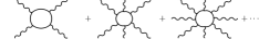
Figure 1: Sum of diagrams equivalent to the one-loop EHL.

If the field has an electric component ($b\neq 0$) then there are poles on the integration contour at $ebT=k\pi$ which create an imaginary part. For the purely electric case one gets Schwinger’s 1951 formula,

$${\rm Im}{\cal L}^{(1)}(E) = \frac{m^{4}}{8\pi^{3}}\beta^{2}\,\sum_{k=1}^{\infty}\frac{1}{k^{2}}\,\exp\left[-\frac{\pi k}{\beta}\right]$$ (2)

($\beta=eE/m^{2}$). In the following we will consider the weak-field limit $\beta\ll 1$, where only the leading $k=1$ is relevant. Note that ${\rm Im}{\cal L}^{(1)}(E)$ depends on $E$ non-perturbatively (nonanalytically), which is consistent with Sauter’s interpretation of pair creation as vacuum tunneling.

This connection between the effective action and the pair creation rate is based on the Optical Theorem, which relates the imaginary part of the diagrams shown in Fig. 1 to the “ cut diagrams ” shown in Fig. 2.

         

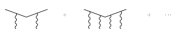
Figure 2: “Cut” diagrams describing Schwinger pair creation.

However, the latter individually all vanish for a constant field, which can emit only zero-energy photons. Thus for a constant field we cannot use dispersion relations for individual diagrams; what counts is the asymptotic behaviour of the diagrams for a large number of photons. The appropriate generalization is a Borel dispersion relation. This works in the following way $\!{{\bf??}}$: define the weak field expansion coefficients of the purely electric EHL by

$${\cal L}^{(1)}(E)=\sum_{n=2}^{\infty}c(n)\Bigl{(}\frac{eE}{m^{2}}\Bigr{)}^{2n}\,.$$ (3)

It can be shown that their leading large - $n$ behavior is

$$c(n)\,\,{\stackrel{{\scriptstyle n\to\infty}}{{\sim}}}\,\,c_{\infty}\Gamma[2n-2]$$ (4)

with a constant $c_{\infty}$. The Borel dispersion relation relates this leading behavior to the leading weak-field behavior of the imaginary part of the Lagrangian:

$${\rm Im}{\cal L}^{(1)}(E)\,\,{\stackrel{{\scriptstyle\beta\to 0}}{{\sim}}}\,\,c_{\infty}\,\,{\rm e}^{-\frac{\pi m^{2}}{eE}}\,.$$ (5)

Thus we have rederived the leading Schwinger exponential of (2) in a way that turns out to be very useful for higher-loop considerations.

The two-loop (one-photon exchange) correction to the EHL corresponds to the set of diagrams shown in Fig. 3 (there is also a one-particle reducible contribution $\!{{\bf??}}$, but for our present purposes it can be discarded). The corresponding corrections to the tree-level pair creation diagrams of Fig. 2 are shown in Fig. 4.

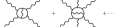
Figure 3: Feynman diagrams corresponding to the 2-loop EHL.

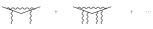
Figure 4: Feynman diagrams contributing to 2-loop Schwinger pair creation.

These two-loop diagrams lead to rather intractable two-parameter integrals $\!{{\bf??},{\bf??}}$. However, the imaginary part ${\rm Im}{\cal L}^{(2)}(E)$ when taken in the weak-field limit becomes a simple addition to ${\rm Im}{\cal L}^{(1)}(E)$ $\!{{\bf??}}$:

$${\rm Im}{\cal L}^{(1)}(E)+{\rm Im}{\cal L}^{(2)}(E)\,\,\,\,{\stackrel{{\scriptstyle\beta\to 0}}{{\sim}}}\,\,\,\,\frac{m^{4}\beta^{2}}{8\pi^{3}}\bigl{(}1+\alpha\pi\bigr{)}\,{\rm e}^{-{\pi\over\beta}}\,.$$ (6)

In $\!{{\bf??}}$, Lebedev and Ritus further noted that, if one assumes that higher orders in this limit will lead to exponentiation,

$${\rm Im}{\cal L}^{(1)}(E)+{\rm Im}{\cal L}^{(2)}(E)+\ldots\,\,\,\,{\stackrel{{\scriptstyle\beta\to 0}}{{\sim}}}\,\,\,\,\frac{m^{4}\beta^{2}}{8\pi^{3}}\,{\rm exp}\Bigl{[}-{\pi\over\beta}+\alpha\pi\Bigr{]}={\rm Im}{\cal L}^{(1)}(E)\,\,{\rm e}^{\alpha\pi}$$ (7)

then the result could be interpreted in the tunneling picture as the corrections to the Schwinger pair creation rate due to the pair being created with a negative Coulomb interaction energy:

$$m(E)\approx m+\delta m(E),\quad\delta m(E)=-\frac{\alpha}{2}\frac{eE}{m}$$ (8)

where $\delta m(E)$ is just the “Ritus mass shift”, originally derived from the crossed process of one-loop electron propagation in the field $\!{{\bf??}}$.

For scalar QED the corresponding exponentiation had been conjectured already two years earlier by Affleck, Alvarez and Manton $\!{{\bf??}}$:

$$\sum_{l=1}^{\infty}{\rm Im}{\cal L}^{(l)}_{\rm scal}(E) {\stackrel{{\scriptstyle\beta\to 0}}{{\sim}}} -\frac{m^{4}\beta^{2}}{16\pi^{3}}\,{\rm exp}\Bigl{[}-{\pi\over\beta}+\alpha\pi\Bigr{]}={\rm Im}{\cal L}^{(1)}_{\rm scal}(E)\,\,{\rm e}^{\alpha\pi}\,.$$ (9)

However, they arrived at this conjecture in a very different way, namely using Feynman’s worldline path integral formalism in a semi-classical approximation.

Thus there is much that speaks for the exponentiation conjecture. However, it would be a very surprising result, since it leads to the analytic factor ${\rm e}^{\alpha\pi}$! This is counter-intuitive, since the growth in the number of diagrams caused by the insertion of an increasing number of photons into an electron loop would lead one to expect a vanishing radius of convergence in $\alpha$.

Using Borel analysis, this factor can be transferred from the imaginary part of the effective Lagrangian to the large - $N$ limit of the $N$ - photon amplitudes $\!{{\bf??}}$:

$${\rm lim}_{N\to\infty}\frac{\Gamma^{({\rm all-loop})}[k_{1},\varepsilon_{1};\ldots;k_{N},\varepsilon_{N}]}{\Gamma^{(1)}[k_{1},\varepsilon_{1};\ldots;k_{N},\varepsilon_{N}]}=\,{\rm e}^{\alpha\pi}\,$$ (10)

The exponentiation conjecture has been verified at the two-loop order by explicit computation in both scalar and spinor QED. A three-loop check in $D=4$ seems presently out of reach. In 2005, Krasnansky $\!{{\bf??}}$ found the following explicit formula for the two-loop EHL in scalar QED in 1+1 dimensions:

$${\cal L}_{\rm scal}^{(2)(2D)}(\kappa) = -\frac{e^{2}}{32\pi^{2}}\left(\xi^{2}_{2D}-4\kappa\xi_{2D}^{\prime}\right),$$ (11)

where $\xi_{2D}=-\Bigl{(}\psi(\kappa+{1\over 2})-\ln(\kappa)\Bigr{)}$, $\psi(x)=\frac{\Gamma^{\prime}(x)}{\Gamma(x)}$, $\kappa=\frac{m^{2}}{2ef}$, $f^{2}={1\over 4}F_{\mu\nu}F^{\mu\nu}$.

This is simpler than in four dimensions, but still non-trivial (in fact very similar in structure to the EHL in four dimensions for a self-dual field $\!{{\bf??}}$), which suggests to use 1+1 dimensional QED as a toy model for testing the exponentiation conjecture. In $\!{{\bf??}}$ we used the method of $\!{{\bf??}}$ to generalize the exponentiation conjecture to the 2D case, obtaining

$${\rm Im}{\cal L}^{(all-loop)}_{2D}\sim\,{\rm e}^{-\frac{m^{2}\pi}{eE}+\tilde{\alpha}\pi^{2}\kappa^{2}}$$ (12)

where $\tilde{\alpha}=\frac{2e^{2}}{\pi m^{2}}$, and obtained the one- and two-loop $2D$ spinor QED EHL explicitly in terms of the function $\tilde{\psi}(x)\equiv\psi(x)-\ln x+{1\over 2x}$. This allowed us to obtain formulas for $c^{(1,2)}(n)$ in terms of the Bernoulli numbers, and made it possible to analytically verify (12) at the two-loop level:

$$\lim_{n\to\infty}{c^{(2)}(n)\over c^{(1)}(n+1)} = \tilde{\alpha}\pi^{2}\,.$$ (13)

At the three-loop level, only the two diagrams with a single electron loop, Fig. 5, turn out to be relevant for the exponentiation conjecture.

Figure 5: Single electron-loop contributions to the three-loop EHL.

In $\!{{\bf??}}$ the authors developed a method for computing the weak-field expansion coefficients for these diagrams, and obtained the first seven coefficients explicitly; one more was computed by E. Panzer. Plotting these eight coefficients, one gets Fig. 6, where the normalization is such that the coefficients would have to converge to unity for the conjecture to hold at the three-loop level, which appears unlikely.

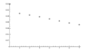
Figure 6: Plot of the three-loop coefficients against the asymptotic prediction.

To summarize:

• The higher-loop corrections to the one-loop Euler-Heisenberg Lagrangian should provide valuable information on the asymptotic properties of QED.

• The exponentiation conjecture implies two very non-obvious properties of the asymptotic growth of the weak-field expansion coefficients: (i) At any fixed loop order, their leading asymptotic growth is always the same (which already at the two-loop level is true only after renormalization!). (ii) The coefficients of these leading terms exponentiate in $\alpha$.

• The exponentiation in $\alpha$ seems not to be true (at least not for $D=2$), but analyticity in $\alpha$ remains a strong possibility.

References

- [1] G.V. Dunne, C. Schubert, Nucl. Phys. B 564 (2000) 59.
- [2] H. Gies, F. Karbstein, JHEP 1703 (2017) 108.
- [3] V. I. Ritus, Zh. Eksp. Teor. Fiz 69 (1975) 1517 [Sov. Phys. JETP 42 (1975) 774].
- [4] S. L. Lebedev, V. I. Ritus, Zh. Eksp. Teor. Fiz. 86 (1984) 408 [JETP 59 (1984) 237].
- [5] V.I. Ritus, Zh. Eksp. Teor. Fiz. 75 (1978) 1560 [JETP 48 (1978) 788].
- [6] I.K. Affleck, O. Alvarez, N.S. Manton, Nucl. Phys. B 197 (1982) 509.
- [7] G.V. Dunne, C. Schubert, J. Phys.: Conf. Ser. 37 (2006) 59.
- [8] M. Krasnansky, Int. J. Mod. Phys. A 23, 5201 (2008).
- [9] G. V. Dunne, C. Schubert, JHEP 0208 (2002) 053.
- [10] I. Huet, D.G.C. McKeon, C. Schubert, JHEP 1012 (2010) 036.
- [11] I. Huet, M. Rausch de Traubenberg, C. Schubert, JHEP 1903 (2019) 167.