On the Universal Texture in the PA-2HDM for the V-SPIN case

Abstract

In a Partially Aligned Two Higgs Doublet Model, where only is allowed flavor violation between third and second generation of fermions, we propose a mechanism to generate the second Yukawa matrix through a Unitary V-Spin flavor transformation on the mass matrix for quarks and leptons. Also we assume that this flavor transformation is universal, this is, we use the same parameters to generate Yukawa matrix elements in both sectors, reducing drastically the number of free parameters. As consequence we obtained a serie of relations between Yukawa matrix elements, that we called the Universality Constraint. Also, we obtained an interval of values for the second Yukawa matrix elements, expressed in terms of the Cheng and Sher ansatz, for $\tau\to\mu\mu^{+}\mu^{-}$ and $\tau\to\gamma\mu$ coming from the Universality Constraint and experimental bounds for light scalar masses. Finally, we show the allowed region of parameters for the flavor transformation from $B_{s}\to\mu\mu$ decays, $B_{s}^{0}-\bar{B}_{s}^{0}$ mixing, $\tau\to\mu\mu^{+}\mu^{-}$ and $\tau\to\gamma\mu$ experimental bounds.

PACS numbers:11.30.Hv, 12.15.Ff, 13.20.-v, 14.80Cp

1 Introduction

After the 2012 discovery of the Higgs boson, particle physics entered a new era. On one hand, the Standard Model (SM) predictions have been confirmed with remarkable precision, reinforcing its role as the best description of nature up to the electroweak scale. On the other hand, there are many open questions from the theoretical and phenomenological points of view, and some tension in the experimental measurements related to some rare meson decays. At present, we do not have a deep understanding of the matter sector of the SM, its familiar multiplicity and hierarchical couplings, nor can we explain the amount of baryonic asymmetry and the abundance and nature of dark matter. Beyond the SM, theories with Natural Flavor Conservation are unable to account for various tensions between the SM and Lepton Flavor Violation (LFV), polarization asymmetries, etc. At the same time, many observables constrain the apparition of Flavor Changing Neutral Currents (FCNCs), which should be very small[1].

An interesting feature of the SM as it stands today is that the mixing structures of quarks and leptons are notably different: neutrino mixing is very large compared with quark mixing, where the offline CKM entries are significantly supressed. This appears to suggest that different mechanisms may account for lepton and quarks mass generation and mixings. For example, this happens in models that couple the light and heavy fermions to different Higgs doublets[2]. Another interesting possibility is the existence of Majorana mass terms in the neutrino sector, which would provide a clear difference between quarks and leptons[3].

However, apparently different mixing structures in the leptonic and quark sectors, can be accomodated with the same structure at the price of leaving the fermion masses unexplained. This is the idea of a universal texture [4, 5], where the mass hierarchy is responsible for the nearly maximal neutrino mixing and the suppressed quark mixing angles. In this scenario, only the mixing is addressed since the lepton and quark mass hierarchy remains unexplained, although it is possible to implement such hierarchy with a Froggat-Nielsen mechanism [6]. Nonetheless, while representing only a partial solution, this would still be a step forward.

The present work explores this concept by pitting a version of the universal texture idea against the significant constraints coming from rare lepton and meson decays. In a previous work[7], a version of the 2HDM was studied where Yukawa matrices are almost-aligned in such a way that only a pair of generations at a time develops FCNC’s. We will refer to this model as the Partially Aligned Two Higgs Doublet Model (PA-2HDM) [8], and focus in an scenario with second and third family mixing, called the V-spin. In order to implement the universal texture idea, the same dimensionless parameters are used for the quark and lepton Yukawa couplings, with scales provided by the fermion masses.

In the following, section 2 lays out the model and the assumptions employed. In section 3, some rare decays are used to test the viability of the model and we show our numerical analysis. Afterwards, we present our conclusions in section 4.

2 The V-Spin case of the PA-2HDM and the Universality Constraint

The starting point of the PA-2HDM is a generic 2HDM that might be seen as a low energy limit of a model with an underlying flavor dynamics. The Yukawa sector of the 2HDM has the following form

$$-\mathcal{L}_{Y} = \bar{Q}_{Li}\left[Y^{d}_{a,ij}\Phi_{a}D_{Rj}+Y^{u}_{a,ij}\tilde{\Phi}_{a}U_{Rj}\right]$$ (1)

$$+\bar{L}_{Li}Y_{a,ij}^{\ell}\Phi_{a}E_{Rj}+\text{H.c.},$$

where $i,j$ are flavor indexes and $a=1,2$. $Q_{Li}=(U_{Li},D_{Li})$ and $L_{Li}=(N_{Li},E_{Li})$ are the fermion $SU(2)$ doublets, and $D_{Rj}$, $U_{Rj}$ and $E_{Rj}$ are the fermion singlets. The mass matrix is defined by

$$M^{f}_{ij}=\frac{1}{\sqrt{2}}\left(v_{1}Y^{f}_{1,ij}+v_{2}Y^{f}_{2,ij}\right),$$ (2)

where $f=u,d,\ell$ or $e,\mu,\tau$, and $v_{1}$ and $v_{2}$ are the vacuum expectation values (VEV) of each doublet. There are several ways to parameterize flavor violating (FV) couplings. In this work, to ease comparison with the literature, we use (2) to write down the Feynman rules in terms of the mass matrix $M^{f}_{ij}$, and $Y^{f}_{2,ij}$ for the couplings of down-type quarks and leptons. Once the mass matrix is diagonal in the mass basis, the matrix $Y^{f}_{2,ij}$ contains all information of the FV contribution.

We express the Yukawa matrix elements in the Cheng and Sher ansatz [9], but relaxing the requirement of order-one couplings $\chi^{f}_{2,ij}$:

$$Y^{f}_{2,ij}=\frac{\sqrt{m^{f}_{i}m^{f}_{j}}}{v}\chi^{f}_{2,ij},\quad\text{for}\quad f=d,\ell.$$ (3)

Here, the parameters $\chi^{f}_{2,ij}$ can take any complex value. Without loss of generality, we can parameterize these contributions as follows:

$$\chi_{2,ij}^{f}=\frac{1}{\sqrt{m^{f}_{i}m^{f}_{j}}}\left(A^{f}_{2L}M^{f}A_{2R}^{f}\right)_{ij},$$ (4)

where $v^{2}=v_{1}^{2}+v_{2}^{2}$ and $A_{2L(R)}^{f}$ are $SU(3)$ matrices.

Alignment between the Yukawa couplings[10] is one of several ways to constrain the large number of parameters of the 2HDM-III[11]. As it was described before, the PA-2HDM relaxes the alignment in order to generalize the model while keeping the free parameters manageable. In this work, we will focus in a version of the PA-2HDM where only the mixing between the second and the third generation of quarks and leptons is allowed. We consider this to be the most promising case given the experimental constraints. For example, the $K^{0}-\bar{K}^{0}$ mixing is very close to the SM prediction, and therefore permits a very restricted NP contribution [12]. In the leptonic $\tau$ decays and $\mu$ decays recently updated upper bounds are given by [1, 13]

$$\text{Br}(\mu\to ee^{+}e^{-}) <1.0\times 10^{-12},$$ (5)

$$\text{Br}(\mu\to e\gamma\gamma) <1.0\times 10^{-12},$$ (6)

$$\text{Br}(\tau\to\mu e^{+}e^{-}) <1.8\times 10^{-8},$$ (7)

$$\text{Br}(\tau\to\mu\gamma) <4.4\times 10^{-8},$$ (8)

$$\text{Br}(\mu\to e\gamma) <4.2\times 10^{-13}.$$ (9)

The flavor changing (FC) upper bounds for $\tau$-$\mu$ are up to five orders of magnitude larger than $\mu$-$e$ bounds. If we include the FC processes $\tau$-$e$, we have bounds similar to $\tau$-$\mu$. Modulo kinematical effects, the mixing of any generation with the third generation prevails over the one that first and second mixing. Now, if we observe the leptonic decays[1]

$$\text{Br}(B_{s}^{0}\to\mu\bar{\mu})=(3.0\pm 0.4)\times 10^{-9},$$ (10)

$$\text{Br}(B_{d}^{0}\to\mu\bar{\mu})=(1.4^{+1.6}_{-1.4})\times 10^{-10},$$ (11)

the FV process for $b-s$ mixing is one order of magnitude larger than the $b-d$ one. Since we want to find a common mixing texture for leptons and quarks, this favors choosing the PA-2HDM version with mixing of the second and third generations. We call the choice to enforce a universal texture the Universality Constraint(UC). Having taken observations on the current experimental evidence, and considering that we are looking for a scenario with light pseudoscalar and scalars, we will from now on consider the PA-2HDM with $\chi^{q,\ell}_{2,1j}\simeq 0$ and $j=(2,3)$, the V-Spin scenario.

In order to analyze the consequences of the UC and its phenomenological viability, we have chosen a set of channels where FCNC and LFV couplings appear either at tree level (in the case of $B_{s}^{0}\to\mu\bar{\mu}$, $B^{0}_{s}-\bar{B}^{0}_{s}$ physics), or at least at one and two loops (for $\tau\to\mu\ \mu^{+}\mu^{-}$, $\tau\to\gamma\mu$). In Table 2, we show the experimental values for the branching ratios and the SM bounds. The $\tau$ channels are promising since the corresponding SM contribution is extremely small.

Channels with Flavor Violation where only couplings of the second and third generation $\chi_{2,ij}^{q,\ell}$ are involved. Channel SM prediction Exp. Results [1] $\text{BR}(\tau\to\gamma\mu)$ $<10^{-53}$ [14, 15] $<4.4\times 10^{-8}$ $\text{BR}(\tau\to\mu\mu^{+}\mu^{-})$ $6.4\times 10^{-55}$ [16] $<2.1\times 10^{-8}$ $\text{BR}(B_{s}^{0}\to\mu^{+}\mu^{-})$ $(3.65\pm 0.23)\times 10^{-9}$ [17] $(3.0\pm 0.4)\times 10^{-9}$ $\Delta M_{B^{0}_{s}}\ (\times 10^{-8}\text{MeV})^{-1}$ $(1.3167\pm 0.08225)$ [18] $(1.169\pm 0.0014)$

Because we have chosen the V-Spin scenario, as discussed in a previous work[7], channels with FCNC and LFV involving fermions of the first generation do not get NP contributions. Therefore, the compatibility between the SM predictions and the experimental data will not be altered. Also, the values for flavor-conserving parameters $\chi^{\ell,q}_{2,ii}$ are not strongly constrained.

The observations described above are similar to those that sustain the approximations taken long time ago in the context of the 2HDM-III as in reference [19], or even to ignore the tree level FC coupling in [20], to mention some examples. In contrast, in this work we assume that the absencet of FC couplings at tree level involving the first generation of fermions is consequence of an underlying flavor symmetry in the context of a generic 2HDM.

For the V-Spin texture, we can rewrite the couplings in terms of the parameters $(c^{V}_{0},c^{V}_{3},c^{V})$ and the angle $\theta_{V}$:

$$\tilde{\chi}^{f}_{2,11} = (c^{V}_{0})^{2},$$ (12)

$$\tilde{\chi}^{f}_{2,22} = (c^{V}_{0}+c^{V}_{3})^{2}+\frac{m^{f}_{3}}{m_{2}^{f}}(c^{V})^{2},$$ (13)

$$\tilde{\chi}^{f}_{2,33} = (c^{V}_{0}-c^{V}_{3})^{2}+\frac{m^{f}_{2}}{m_{3}^{f}}(c^{V})^{2},$$ (14)

$$\tilde{\chi}^{f}_{2,23} = c^{V}e^{i\theta_{V}}\left[\sqrt{\frac{m^{f}_{2}}{m_{3}^{f}}}(c^{V}_{0}+c^{V}_{3})+\sqrt{\frac{m^{f}_{3}}{m^{f}_{2}}}(c^{V}_{0}-c^{V}_{3})\right],$$ (15)

with $\tilde{\chi}_{2,13}^{f}=\tilde{\chi}_{2,12}^{f}=0$.

This same structure, with the same values for the $c^{V}$, $c_{0}^{V}$ and $c_{3}^{V}$ parameters, is used for the leptonic and quark sectors.

3 Rare $\tau$ decays and FCNC for $B_{s}^{0}$ in the V-Spin texture

3.1 The observables for the V-Spin texture

In the PA-2HDM for the V-Spin case, the only channels with LFV are those that involve the $\tau$ and $\mu$ leptons. We will consider the decays of $\tau$ leptons that appear in Table 2 in order to test our hypothesis about the viability of the reduction of free parameters.

3.1.1 The $\tau\rightarrow\mu\gamma$ channel

For $\tau\rightarrow\mu\gamma$, the SM prediction is too small to be experimentally accesible[16], while the experimental bound is many orders of magnitude above[21]. This bound is expected to improve one order of magnitude during the current LHC era[22]. The Bjorken-Weinberg mechanism can make the two loops correction larger than the one loop contribution[23]. This effect is more pronounced in the higher mass region. Here, we are mainly interested in relatively light new scalars from the 2HDM, where the two-loops contribution is not too important, nevertheless we will consider it in our numerical calculations. Also, as this decay has been measured with very good precision, we use the exact 2-loops expression given by[24, 25]

$$\mathcal{M} \simeq \frac{1}{16\pi^{2}}\left\{\sqrt{2}\sum_{\phi}\frac{\Gamma_{\phi\mu\tau}\Gamma_{\phi\tau\tau}}{M_{\phi}^{2}}\left(\log\frac{M_{\phi}^{2}}{m_{\tau}^{2}}-\frac{3}{2}\right)\right.$$ (16)

$$\quad\left.+2\sum_{\phi,f}\Gamma_{\phi\mu\tau}\Gamma_{\phi ff}\frac{N_{c}Q_{f}^{2}\alpha}{\pi}\frac{1}{m_{\tau}m_{f}}F_{\phi}\left(\frac{m_{f}^{2}}{M_{\phi}^{2}}\right)\right.$$

$$\left.\qquad-\sum_{h^{0},H^{0}}\Gamma_{\phi\mu\tau}C_{\phi WW}\frac{g\alpha}{2\pi m_{\tau}M_{W}}\left[3F_{\phi}\left(\frac{M_{W}^{2}}{m_{\phi}^{2}}\right)\right.\right.$$

$$\qquad\left.\left.+\frac{23}{4}G\left(\frac{M_{W}^{2}}{M_{\phi}^{2}}\right)+\frac{3}{4}H\left(\frac{M_{W}^{2}}{M_{\phi}^{2}}\right)+M_{\phi}^{2}\frac{F_{\phi}\left(\frac{M_{W}^{2}}{M_{\phi}^{2}}\right)-G\left(\frac{M_{W}^{2}}{M_{\phi}^{2}}\right)}{2M_{W}^{2}}\right]\right\}$$

where $\phi=h^{0},H^{0},A^{0}$ and $f=t,b$ . The loops integrals can be written as[24]

$$F_{A}(z) = G(z)=\frac{z}{2}\int^{1}_{0}dx\frac{1}{x(1-x)-z}\log\left[\frac{x(1-x)}{z}\right],$$ (17)

$$F_{h^{0},H^{0}} = \frac{z}{2}\int^{1}_{0}dx\frac{(1-2x(1-x))}{x(1-x)-z}\log\left[\frac{x(1-x)}{z}\right],$$ (18)

$$H(z) = -\frac{z}{2}\int^{1}_{0}dx\frac{1}{x(1-x)-z}\left\{1-\frac{z}{x(1-x)-z}\log\left[\frac{x(1-x)}{z}\right]\right\}.$$ (19)

In these expressions, only the 2-loop contributions coming from virtual $t$ and $b$ quarks have been considered.

The couplings for the PA-2HDM are obtained from (3) and (15). In this model, the couplings of gauge bosons with the scalars $H^{0}$ and $h^{0}$ are the same as in Ref. [25]:

$$C_{h^{0}WW} = \sin(\beta-\alpha),$$ (20)

$$C_{H^{0}WW} = \cos(\beta-\alpha).$$ (21)

The branching ratio for this decay is a function of the scalar masses, $\tan\beta$, the angle $\alpha$ and the $c^{\prime}s$ parameters through the $\chi^{\ell}_{2,\tau\mu}$ and $\chi^{\ell}_{2,\tau\tau}$ couplings. In order to test the V-Spin texture and compute our numerical estimations we have fixed $\alpha=0$ and set relatively light scalar masses; i. e. $M_{H^{0}}=300$ GeV and $M_{A^{0}}=300$. For the light scalar $h^{0}$, we have fixed its mass as $125.6$ GeV. In Figure 1, we show the allowed regions in the parameter space $\chi^{\ell}_{2,\tau\mu}$ vs $\chi^{\ell}_{2,\tau\tau}$ that are compatible with the experimental upper bound of $\text{Br}(\tau\to\gamma\mu)$ for different values of $\tan\beta$. Also, we plot the restricted region that comes from the UC, that is, the restriction coming from the expressions (12-15). As it can be seen in the graph, for small values of $|\chi^{\ell}_{2,\tau\tau}|$ the upper bound of $\chi^{\ell}_{2,\tau\mu}$ is determined by the UC and the allowed region is smaller than the one without V-Spin texture.

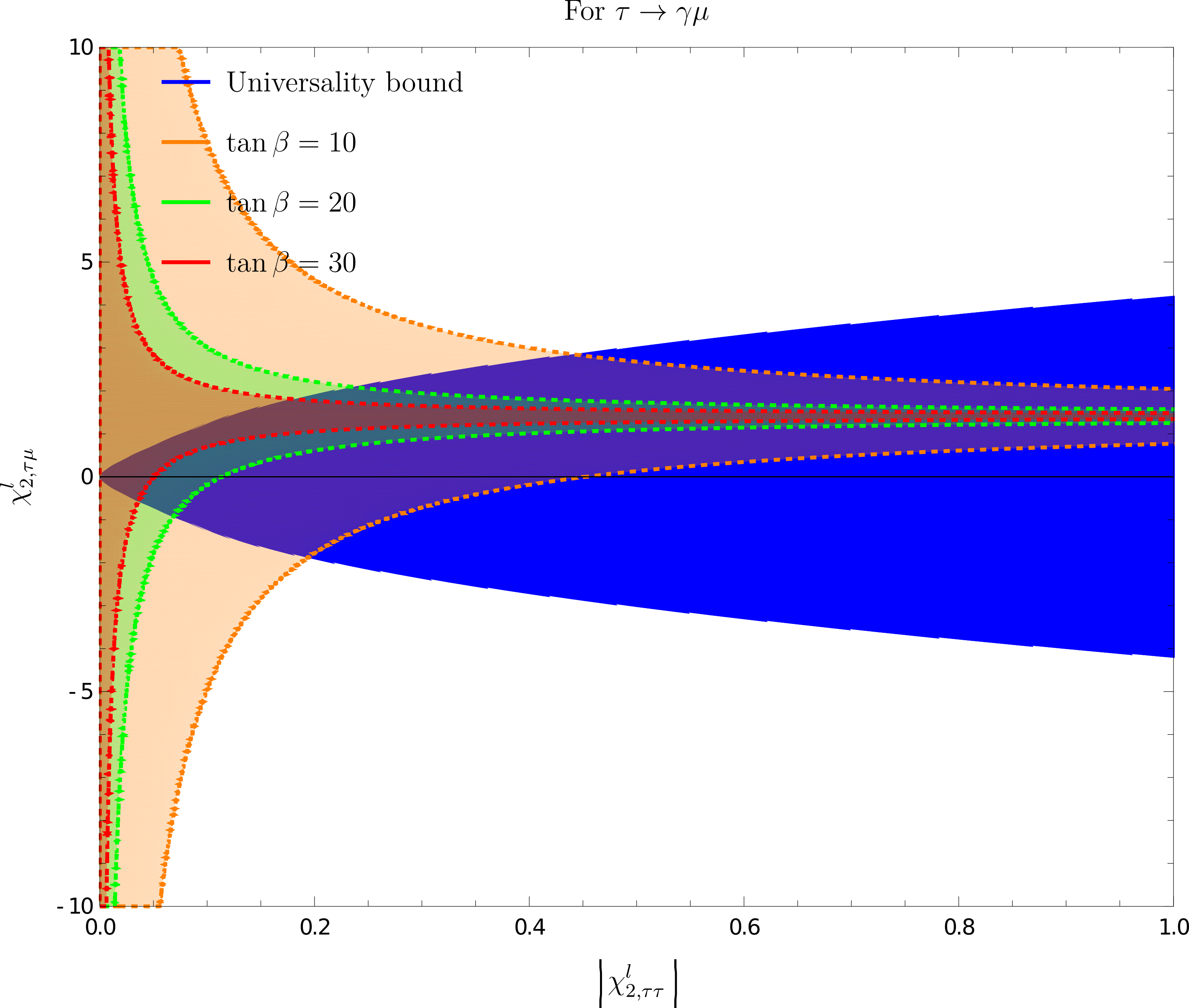
Figure 1: Alowed regions for $\chi^{\ell}_{2,\tau\mu}$ and $|\chi^{\ell}_{2,\tau\tau}|$ with masses $m_{h}=125.6$ GeV, $M_{H^{0}}=300$ GeV and $M_{A^{0}}=300$ GeV and several values of $\tan\beta$. Constrictions come from the $\tau\to\gamma\mu$ experimental bound and from the UC hypothesis.

3.1.2 The channel $\tau\to 3\mu$

In the SM, the $\tau\to\mu\mu^{+}\mu^{-}$ decay is strongly suppressed because the main contribution comes from higher order diagrams suppressed by a GIM-like mechanism[16]. In order to estimate the NP contribution to this channel, we dismiss the SM contribution and adopt the formalism of the Effective Lagrangians [26, 27]. In general, the amplitude for this channel from scalar contributions can be written as

$$\mathcal{L}_{\text{eff}} \simeq C_{\tau\mu\mu\mu}^{LL}\left(\bar{\mu}P_{L}\tau\right)\left(\bar{\mu}P_{L}\mu\right)+C_{\tau\mu\mu\mu}^{RR}\left(\bar{\mu}P_{R}\tau\right)\left(\bar{\mu}P_{R}\mu\right)$$ (22)

$$+C_{\tau\mu\mu\mu}^{LR}\left(\bar{\mu}P_{L}\tau\right)\left(\bar{\mu}P_{R}\mu\right)+C_{\tau\mu\mu\mu}^{RL}\left(\bar{\mu}P_{R}\tau\right)\left(\bar{\mu}P_{L}\mu\right)$$

where the Wilson coefficients are defined by

$$C_{\tau\mu\mu\mu}^{Q_{1}Q_{2}}=-i\sum_{\phi}\frac{\Gamma_{\phi\tau\mu}^{Q_{1}}\Gamma_{\phi\mu\mu}^{Q_{2}}}{M_{\phi}^{2}}$$ (23)

with $Q_{1}=L,R$ and $Q_{2}=L,R$ and $\phi=h^{0},H^{0},A^{0}$. The couplings obtained from the Lagrangian (1) using the parametrization described in section 2 are

$$\Gamma^{R(L)}_{h^{0}\ell_{i}\ell_{j}} = +(-)i\left[\frac{\cos(\alpha-\beta)}{v\cos\beta}\delta_{ij}m_{\ell_{i}}-\frac{\sin\alpha}{\sqrt{2}\cos\beta}Y^{\ell}_{2,ij}(c^{V},c_{0}^{V},c_{3}^{V})\right]$$ (24)

$$\Gamma^{R(L)}_{H^{0}\ell_{i}\ell_{j}} = +(-)i\left[\frac{\sin(\alpha-\beta)}{v\cos\beta}\delta_{ij}m_{\ell_{i}}+\frac{\cos\alpha}{\sqrt{2}\cos\beta}Y^{\ell}_{2,ij}(c^{V},c_{0}^{V},c_{3}^{V})\right]$$ (25)

$$\Gamma^{R(L)}_{A^{0}\ell_{i}\ell_{j}} = -\left[\frac{\tan\beta}{v\cos\beta}\delta_{ij}m_{\ell_{i}}-\frac{1}{\sqrt{2}\cos\beta}Y^{\ell}_{2,ij}(c^{V},c_{0}^{V},c_{3}^{V})\right]$$ (26)

where the matrices $Y^{\ell}_{2,ij}$ are hermitian. Thus, the squared amplitude takes the following form

$$|\mathcal{M}|^{2} = 4\left[\frac{1}{4}(m^{2}_{23}-2m_{\mu}^{2})(m_{\tau}^{2}+m_{\mu}^{2}-m_{23}^{2})F_{1}+m_{\tau}m_{\mu}(m_{23}^{2}-2m_{\mu}^{2})F_{2}\right.$$ (27)

$$+m_{\mu}^{2}(-m_{23}^{2}+m_{\tau}^{2}+m_{\mu}^{2})F_{3}+2m_{\tau}m_{\mu}^{3}F_{4}\Big{]}$$

where $m_{23}^{2}=(p_{2}+p_{3})^{2}$ and $p_{2,3}$ are the 4-momentum of the final muons. The parameters $F_{i}$ are in general

$$F_{1} = |C^{LL}_{\tau\mu\mu\mu}|^{2}+|C^{LR}_{\tau\mu\mu\mu}|^{2}+|C^{LR}_{\tau\mu\mu\mu}|^{2}+|C^{RL}_{\tau\mu\mu\mu}|^{2},$$ (28)

$$F_{2} = \text{Re}\left(C^{RL}_{\tau\mu\mu\mu}C^{LL*}_{\tau\mu\mu\mu}+C^{RR}_{\tau\mu\mu\mu}C^{LR*}_{\tau\mu\mu\mu}\right),$$ (29)

$$F_{3} = \text{Re}\left(C^{LR}_{\tau\mu\mu\mu}C^{LL*}_{\tau\mu\mu\mu}+C^{RR}_{\tau\mu\mu\mu}C^{RL*}_{\tau\mu\mu\mu}\right),$$ (30)

$$F_{4} = \text{Re}\left(C^{RR}_{\tau\mu\mu\mu}C^{LL*}_{\tau\mu\mu\mu}+C^{RL}_{\tau\mu\mu\mu}C^{LR*}_{\tau\mu\mu\mu}\right).$$ (31)

With the amplitude (27), we have calculated the branching ratio of the $\tau\to 3\mu$ channel. Figure 2 shows the experimentally allowed regions for this channel in the parameter space $\chi^{\ell}_{2,\mu\mu}$ vs $\chi^{\ell}_{2,\tau\mu}$. Also, we have set the theoretical restriction coming from the UC. The region of parameters are consistent with similar analysis in the context of the 2HDM-III[11].

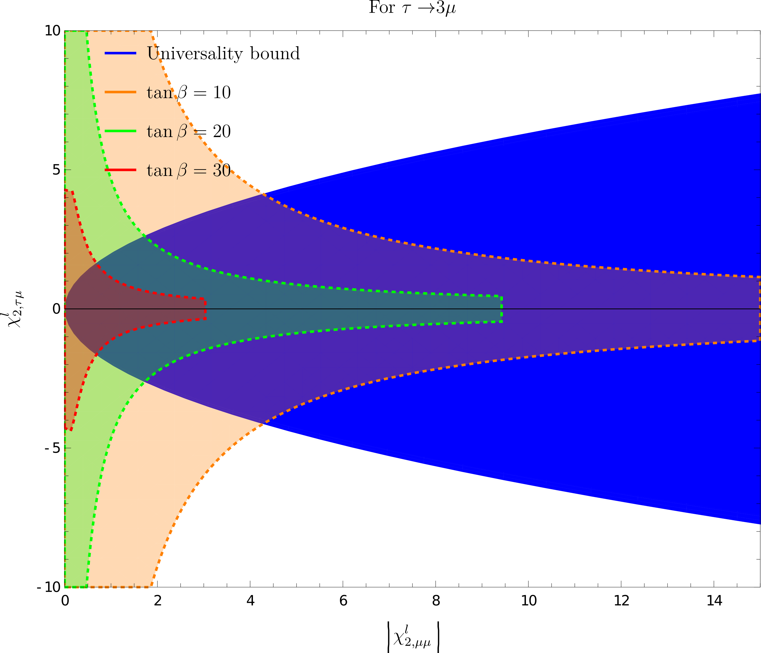
Figure 2: Here, it is shown the allowed values for $\chi^{\ell}_{2,\tau\mu}$ and $|\chi^{\ell}_{2,\mu\mu}|$ for different values of $\tan\beta$ and masses $M_{h^{0}}=125.6$ GeV, $M_{H^{0}}=300$ GeV and $M_{A^{0}}=300$ GeV. Also it is shown the UC coming from the assumption of a common V-Spin texture. As we can see, for small values of $|\chi^{\ell}_{2,\mu\mu}|$ the main restriction on $\chi^{\ell}_{2,\tau\mu}$ comes from the UC and there is a significant reduction of the allowed region.

The interval for $|\chi^{\ell}_{2,\tau\mu}|$ is determined by the upper bound for the branching ratio. We have obtained a similar behavior to the case $\tau\to\gamma\mu$, where we notice that for small values of $|\chi^{\ell}_{2,\mu\mu}|$ the UC is more important than the limit obtained from the experimental measurement. Thus, the LFV contribution is suppressed by the texture given by the expressions (12-15). Comparing the interval of values for $\chi^{\ell}_{2,\tau\mu}$ in Figure 1 and 2, we can see that the UC is more restrictive for the channel $\tau\to\gamma\mu$ than for $\tau\to 3\mu$. Thus, in order to test the UC, the process $\tau\to\gamma\mu$ is more important.

3.1.3 The $B^{0}_{s}\to\mu^{+}\mu^{-}$ channel

This channel is a rare decay because in the SM it is helicity suppressed and it contains FCNC[28, 17]. Since the observation of this decay[29, 30] and its compatibility with the SM prediction[31], it has been used to test several models[32, 33], from the 2HDM [34] to Supersymmetry (See [35] and references therein) and also models with Spin 2 mediators [36] and leptoquarks[37] to mention some examples. A recent experimental study for this decay can be seen in reference [38].

In general, the Wilson operators that contribute to leptonic decays of pseudoscalar mesons at low energies consider whether axial, vector, scalar and pseudoscalar operators [39]. In a general 2HDM, the NP contributions to these decays are only the axial and the pseudoscalar when we restrict ourselves to tree level[34]. The Wilson operators that parameterize such effects are

$$\begin{split}\mathcal{O}_{A}^{q_{f}q_{i}}&=\left(\bar{q}_{f}\gamma_{\mu}P_{L}q_{i}\right)\left(\bar{l}_{B}\gamma^{\mu}\gamma_{5}l_{A}\right),\\ \mathcal{O^{{}^{\prime}}}_{A}^{q_{f}q_{i}}&=\left(\bar{q}_{f}\gamma_{\mu}P_{R}q_{i}\right)\left(\bar{l}_{B}\gamma^{\mu}\gamma_{5}l_{A}\right),\\ \mathcal{O}_{P}^{q_{f}q_{i}}&=\left(\bar{q}_{f}P_{L}q_{i}\right)\left(\bar{l}_{B}\gamma_{5}l_{A}\right),\\ \mathcal{O^{{}^{\prime}}}_{P}^{q_{f}q_{i}}&=\left(\bar{q}_{f}P_{R}q_{i}\right)\left(\bar{l}_{B}\gamma_{5}l_{A}\right).\end{split}$$ (32)

Thus, the effective Hamiltonian is given by

$$\begin{split}\mathcal{H}_{eff}=-\frac{G_{F}^{2}M_{W}^{2}}{\pi^{2}}[C_{V}^{q_{f}q_{i}}O_{V}^{q_{f}q_{i}}+C_{A}^{q_{f}q_{i}}O_{A}^{q_{f}q_{i}}+C_{S}^{q_{f}q_{i}}O_{S}^{q_{f}q_{i}}+C_{P}^{q_{f}q_{i}}O_{P}^{q_{f}q_{i}}\\ +\text{primed}]+H.c..\end{split}$$ (33)

The branching ratio for this decay is reduced to

$$\begin{split}\text{Br}[P^{0}_{\bar{q}_{f},q_{i}}\to l_{A}^{+}l_{B}^{-}]&=\frac{G_{F}^{4}M_{W}^{4}}{32\pi^{5}}f(x_{A}^{2},x_{B}^{2})M_{P^{0}}f_{P^{0}}^{2}(m_{l_{A}}+m_{l_{B}})^{2}\tau_{P^{0}}[1-(x_{A}-x_{B})^{2}]\\ &\left|\frac{M_{P^{0}}^{2}\left(C_{P}^{q_{f}q_{i}}-C_{p}^{{}^{\prime}q_{f}q_{i}}\right)}{\left(m_{q_{f}}+m_{q_{i}}\right)\left(m_{l_{A}}+m_{l_{B}}\right)}-\left(C_{A}^{q_{f}q_{i}}-C_{A}^{{}^{\prime}q_{f}q_{i}}\right)\right|^{2},\end{split}$$ (34)

where $f(x_{i},x_{j})$ is the kinematical function defined by

$$f(x_{i},x_{j})=\sqrt{1-2\left(x_{i}+x_{j}\right)+\left(x_{i}-x_{j}\right)^{2}},$$ (35)

where $x_{i}=\frac{m_{l_{i}}}{M_{P^{0}}}$. The SM contributions to the branching ratio are contained in the Wilson coefficient $C_{A}$. The SM contribution for this channel has been calculated for the pseudoscalar meson $B$ in [40, 41, 42]. In general, the axial contributions for a pseudoscalar meson decay can be written as [34]

$$C_{A}^{q_{f}q_{i}}-C_{A}^{{}^{\prime}q_{f}q_{i}}=-V_{tq_{i}}^{*}V_{tq_{f}}Y(\frac{m_{t}^{2}}{M_{W}^{2}})-V_{cq_{i}}^{*}V_{cq_{f}}Y(\frac{m_{c}^{2}}{M_{W}^{2}}),$$ (36)

where $V_{q_{k}q_{l}}$ are the CKM matrix elements and $Y(x)=\eta_{Y}Y_{0}(x)$ is the widely known Inami-Lim function[43], that includes the NLO QCD effects[28] with $\eta_{Y}=1.0113$. The NP tree level contribution is parameterized by the Wilson coefficients

$$C_{P}-C^{\prime}_{P}=\frac{-i}{m_{A}^{2}}\Gamma_{A^{0}q_{i}q_{f}}\Gamma_{A^{0}\ell_{A}\ell_{B}},$$ (37)

where the couplings are given by (26) and

$$\Gamma_{A^{0}q_{f}q_{i}}=\frac{i}{2}\left[-m_{i}\tan\beta\delta_{fi}+\frac{\sqrt{m_{q_{i}}m_{q_{f}}}}{\sqrt{2}\cos\beta}\tilde{\chi}_{2,q_{f}q_{i}}^{d}\right].$$ (38)

As a result, we obtain the branching ratio as a function of the pseudoscalar mass $M_{A^{0}}$, $\tan\beta$, the mixing angle $\alpha$ and the parameters $c^{V},c^{0},c_{3}^{V}$.

3.1.4 $B_{s}^{0}-B_{s}^{0}$ mixing

In the quark sector, the most important restriction to NP that generates FCNCs comes from the mixing of pseudoscalar neutral mesons. Actually, the $K^{0}-\bar{K}^{0}$ highly restricts the contribution that might come from the interaction with the first generation of quarks. In the case when there exist mixing only between second and third generation, the only observable that might be deviated from the SM prediction is $\Delta M_{B^{0}_{s}}$. In our previous work[7], we have shown that it is possible to find a bound on the non standard scalar contribution to this observable assuming that the experimental measurement contains two terms of the form

$$\Delta M_{q}=\Delta M^{\text{SM}}_{q}+\Delta M^{NP}_{q}.$$ (39)

where $\Delta M^{\text{SM}}_{q}$ is the SM prediction and $\Delta M_{q}^{\text{NP}}$ can be parameterized by

$$\Delta M_{q}^{\text{NP}}(\mu)=|C_{\text{NP}}|\frac{M_{B_{q}}^{2}f_{B_{q}}^{2}}{\left[m_{b}(\mu)+m_{q}(\mu)\right]^{2}}\sigma(\mu),$$ (40)

where we have define $\mathcal{\sigma}(\mu)=|-\frac{5}{24}B_{2}(\mu)+\frac{1}{24}B_{3}(\mu)+\frac{1}{24}B_{4}(\mu)+\frac{1}{12}B_{5}(\mu)|$ and $B_{i}(\mu)$ (for $i=2,3,4,5$) are the renormalized bag parameters at the scale $\mu$ ($\mu=m_{b}$)[44, 45, 46]. The coefficient $|C_{\text{NP}}|$ is calculated at the low energy limit of the generic 2HDM and it has the form

$$|C_{\text{NP}}|=\frac{1+\tan^{2}\beta}{2M_{A}^{2}}|\widetilde{Y}_{2,ij}^{q}|,$$ (41)

where $\widetilde{Y}_{2,ij}^{q}$ is the corresponding Yukawa matrix element in the mass basis. Thus, the upper bound for $|\tilde{\chi}^{d}_{2,bq}|$ is given by

$$|\tilde{\chi}^{d}_{2,bq}|\leq\left(\frac{2M_{A}^{2}}{1+\tan^{2}\beta}\right)\frac{v(m_{b}+m_{q})^{2}}{\sqrt{m_{b}m_{q}}M_{B_{q}}^{2}f_{B_{q}}^{2}}\frac{E_{B_{q}}}{\mathcal{\sigma}(m_{b})},$$ (42)

where we have defined the parameter

$$E_{B_{q}}=|\Delta M^{\text{SM}}-\Delta M^{\text{Exp}}|-\sqrt{\delta^{2}(\Delta M^{\text{SM}})+\delta^{2}(\Delta M^{\text{Exp}})}.$$ (43)

3.2 Numerical analysis

In order to find the combination of parameters that is compatible with the UC, that is, the values of $c^{V}$, $c_{0}^{V}$ and $c_{3}^{V}$ that render values for the branching ratios of $\tau\to\gamma\mu$, $\tau\to 3\mu$ and $B^{0}_{s}\to\mu\bar{\mu}$ restricted by the narrow window for NP given by the restriction of $\Delta M_{B^{0}_{s}}$, we built level curves in the free parameters space with the following choice of parameters:

• The lightest scalar $h^{0}$ of the model was chosen as the Higgs boson of the SM, that is, $M_{h^{0}}=125.6$ GeV.

• We are interested only in scenarios with relatively light non standard neutral scalars and pseudoscalars, thus we have set $M_{A^{0}}=300$ GeV and $M_{H^{0}}=300$ GeV.

• The mixing angle was chosen as $\alpha=0$ without loss of generality.

• For the free parameters in the texture, the phase has been set as $\theta_{V}=0$ and the intervals for $c^{V}$, $c_{0}^{V}$ and $c_{3}^{V}$ are determined by the phenomenology of the 4 selected observables.

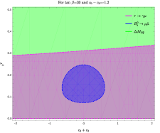
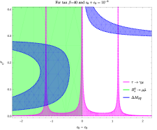
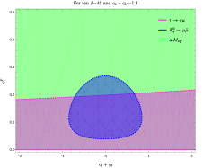
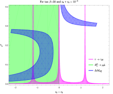
Figure 3: Here, we show the allowed regions of parameters of the transformation (4) that fulfills the experimental bounds coming from the channels $\tau\to\gamma\mu$, $\tau\to 3\mu$ and $B^{0}_{s}\to\mu\bar{\mu}$. Also, it is included the restriction coming from the measurement of $\Delta M_{B^{0}_{s}}$. The region for $\tau\to 3\mu$ is wider and includes the other processes, thus we focus on the regions shown here. On the left, it is shown the narrow region of values for $c_{0}^{V}-c_{3}^{V}$ and $c^{V}$ for different values of $\tan\beta$ with $M_{h^{0}}=125.6$ GeV, $M_{H^{0}}=300$ GeV and $M_{A^{0}}=300$ GeV. The sum of parameters was fixed as $c_{0}^{V}+c_{3}^{V}=10^{-3}$. The right-hand side plots were generated fixing $(c_{0}^{V}-c_{3}^{V})\simeq-1.2$. The area where the allowed region are superposed gives the interval of values for $c^{V}$, $c_{0}^{V}-c_{3}^{V}$ and $c_{0}^{V}+c_{3}^{V}$ where the UC is valid. The region is sensitive to $\tan\beta$ and it disappears at $\tan\beta\gtrsim 80$.

In Figure 3, we look for the region of parameters where UC bound is valid using the 4 channels that contain NP contribution from the V-Spin texture. The region given by $\tau\to 3\mu$ is wider than those from the rest of the processes, thus in the following plot we concentrate our the attention to the region that come from the bounds on $\Delta M_{B^{0}_{s}}$, $\text{BR}(\tau\to\gamma\mu)$ and $\text{BR}(B_{s}^{0}\to\mu\bar{\mu})$. The main result of this work is reviewed in Figure 3, where we have plotted the experimental allowed region described by the parameters $c^{V}$, $c^{V}_{0}-c_{3}^{V}$ and $c^{V}_{0}+c_{3}^{V}$. The left-hand side plots were generated fixing $c_{0}^{V}+c_{3}^{V}\simeq\mathcal{O}(10^{-3})$ . As we can see from the plots on the right side, the only place where there is a superposition of parameters is when $c_{0}^{V}-c_{3}^{V}\simeq-1.2$. This region is very sensitive to the values of $\tan\beta$ and in our analysis we found that for $\tan\beta\gtrsim 80$ the UC coming from the V-Spin cannot describe simultaneously the updated experimental bounds for the three channels with the chosen scalar masses in this analysis.

4 Conclusions

At this point, we want to review this work. We have used the V-Spin case of a PA-2HDM model in order to describe possible FCNC and LFV at tree level as the result of the interchange of non-standard scalars. The V-Spin case gives a texture for the second Yukawa matrix where only the second and the third generation of fermions are mixed. In consequence, only the channels $\tau\to\gamma\mu$, $\tau\to 3\mu$ in the leptonic sector and $B_{s}^{0}\to\mu\bar{\mu}$ with $\Delta M_{B^{0}_{s}}$ for quarks might have effects of NP that could be measured in current experiments.

Also, we have assumed that the texture for the second Yukawa matrix is universal, that is, that the same dimensionless parameters enter the quark and lepton couplings, and the difference in mixings comes from the fermion mass hierarchy. This assumption introduces a relation between the Yukawa matrix elements for different sectors; we have called this relation the Universality Constraint. For this reason, the phenomenological bounds in one sector impacts the predictions for other sectors. In this work, we have used the Cheng and Sher parametrization of the Yukawa matrix elements in order to facilitate a comparison with past analysis on the generic 2HDM and to express the UC in the parameter spaces $\chi^{\ell}_{2,\mu\mu}$ vs $\chi^{\ell}_{2,\tau\mu}$ and $\chi^{\ell}_{2,\mu\mu}$ vs $\chi^{\ell}_{2,\tau\tau}$. This was shown in the figures 2 and 1. These regions were built with the LFV processes $\tau\to\gamma\mu$ and $\tau\to 3\mu$ respectively.

Under the universal texture scheme, the restrictive measurements of B-meson decays require the suppression of LFV effects in $\tau\to\gamma\mu$ and $\tau\to 3\mu$. The allowed regions were shown in Figures 1 and 2 where the superposition region is such that for small values of $\chi^{\ell}_{2,\tau\tau}$ and $\chi^{\ell}_{2,\mu\mu}$, the main restriction on $\chi^{\ell}_{2,\tau\mu}$ comes from the UC. For large values, the experimental bound is stronger for this parameter.

We have found a region in the parameter space where the UC is phenomenologically viable, testing the universality hypothesis using the channels of Table 2. This requires that the dimensionless parameters satisfy $(c_{0}^{V}-c_{3}^{V})\sim-1.2$ and $(c_{0}^{V}+c_{3}^{V})\sim\mathcal{O}(10^{-3})$. The channel $B_{s}^{0}\to\mu\bar{\mu}$ gives the stronger constraint, and updates to experimental precision of this channel could challenge the UC. For relatively light masses $M_{h^{0}}=125.6$ GeV, $M_{H^{0}}=300$ GeV and $M_{A^{0}}=300$ GeV, the allowed region disappear at values of $\tan\beta\gtrsim 80$.

References

- [1] M. Tanabashi et. al., Physical Review D 98, 030001 (Aug 2018), 10.1103/PhysRevD.98.030001.
- [2] W. Altmannshofer and B. Maddock (2018), arXiv:1805.08659, 10.1103/PhysRevD.98.075005.
- [3] G. C. Branco, M. N. Rebelo, J. J. I. Silva-Marcos and D. Wegman, Physical Review D - Particles, Fields, Gravitation and Cosmology 91, 1 (2015), 10.1103/PhysRevD.91.013001.
- [4] Y. Koide, Physical Review D 69, 093001 (May 2004), 10.1103/PhysRevD.69.093001.
- [5] K. Matsuda and H. Nishiura, Physical Review D 69, 053005 (Mar 2004), 10.1103/PhysRevD.69.053005.
- [6] C. D. Froggatt and H. B. Nielsen, Nucl. Phys. B147, 277 (1979), 10.1016/0550-3213(79)90316-X.
- [7] A. Carrillo-Monteverde, S. Gómez-Ávila, R. Gómez-Rosas, L. López-Lozano and A. Rosado, International Journal of Modern Physics A 34, 1950198 (Oct 2019), 10.1142/S0217751X19501987.
- [8] J. Hernández-Sánchez, L. López-Lozano, R. Noriega-Papaqui and A. Rosado, Physical Review D 85, 071301 (Apr 2012), 10.1103/PhysRevD.85.071301.
- [9] T. P. Cheng and M. Sher, Phys. Rev. D35, 3484 (1987), 10.1103/PhysRevD.35.3484.
- [10] A. Pich and P. Tuzon, Phys. Rev. D80, 091702 (2009), arXiv:0908.1554 [hep-ph], 10.1103/PhysRevD.80.091702.
- [11] D. Atwood, L. Reina and A. Soni, Phys. Rev. D55, 3156 (1997), 10.1103/PhysRevD.55.3156.
- [12] A. Antaramian, L. J. Hall and A. Rašin, Physical Review Letters 69, 1871 (Sep 1992), 10.1103/PhysRevLett.69.1871.
- [13] C. O. Dib, T. Gutsche, S. G. Kovalenko, V. E. Lyubovitskij and I. Schmidt, Physical Review D 99, 035020 (Feb 2019), 10.1103/PhysRevD.99.035020.
- [14] B. W. Lee and R. E. Shrock, Physical Review D 16, 1444 (Sep 1977), 10.1103/PhysRevD.16.1444.
- [15] E. . Kou et. al., Progress of Theoretical and Experimental Physics 2019 (Dec 2019), 10.1093/ptep/ptz106.
- [16] G. Hernández-Tomé, G. López Castro and P. Roig, The European Physical Journal C 79, 84 (Jan 2019), 10.1140/epjc/s10052-019-6563-4.
- [17] C. Bobeth, M. Gorbahn, T. Hermann, M. Misiak, E. Stamou and M. Steinhauser, Physical Review Letters 112, 101801 (Mar 2014), 10.1103/PhysRevLett.112.101801.
- [18] L. Di Luzio, M. Kirk and A. Lenz, Physical Review D 97, 095035 (May 2018), 10.1103/PhysRevD.97.095035.
- [19] Z.-j. Xiao and L. Guo, Phys. Rev. D69, 014002 (2004), arXiv:hep-ph/0309103 [hep-ph], 10.1103/PhysRevD.69.014002.
- [20] D. Bowser-Chao, K.-m. Cheung and W.-Y. Keung, Phys. Rev. D59, 115006 (1999), arXiv:hep-ph/9811235 [hep-ph], 10.1103/PhysRevD.59.115006.
- [21] B. Aubert et. al., Physical Review Letters 104, 1 (2010), arXiv:0908.2381, 10.1103/PhysRevLett.104.021802.
- [22] e. Aushev, T. (Feb 2010), arXiv:1002.5012.
- [23] J. D. Bjorken and S. Weinberg, Physical Review Letters 38, 622 (Mar 1977), 10.1103/PhysRevLett.38.622.
- [24] D. Chang, W. S. Hou and W. Y. Keung, Physical Review D 48, 217 (Jul 1993), 10.1103/PhysRevD.48.217.
- [25] S. Davidson and G. Grenier, Physical Review D 81, 095016 (May 2010), 10.1103/PhysRevD.81.095016.
- [26] A. Celis, V. Cirigliano and E. Passemar, Physical Review D 89, 095014 (May 2014), 10.1103/PhysRevD.89.095014.
- [27] C. O. Dib, T. Gutsche, S. G. Kovalenko, V. E. Lyubovitskij and I. Schmidt, Physical Review D 99, 35020 (2019), 10.1103/PhysRevD.99.035020.
- [28] A. J. Buras, J. Girrbach, D. Guadagnoli and G. Isidori, Eur. Phys. J. C72, 2172 (2012), arXiv:1208.0934 [hep-ph], 10.1140/epjc/s10052-012-2172-1.
- [29] LHCb Collaboration (R. Aaij et al.), Phys. Rev. Lett. 110, 021801 (2013), arXiv:1211.2674 [hep-ex], 10.1103/PhysRevLett.110.021801.
- [30] CDF Collaboration (T. Aaltonen et al.), Phys. Rev. D87, 072003 (2013), arXiv:1301.7048 [hep-ex], 10.1103/PhysRevD.97.099901, 10.1103/PhysRevD.87.072003, [Erratum: Phys. Rev.D97,no.9,099901(2018)].
- [31] CMS, LHCb Collaboration (CMS and L. Collaborations) (2013).
- [32] R. Fleischer, Int. J. Mod. Phys. A29, 1444004 (2014), arXiv:1407.0916 [hep-ph], 10.1142/S0217751X14440047.
- [33] D. Guadagnoli and G. Isidori, Phys. Lett. B724, 63 (2013), arXiv:1302.3909 [hep-ph], 10.1016/j.physletb.2013.05.054.
- [34] A. Crivellin, A. Kokulu and C. Greub, Phys. Rev. D87, 094031 (2013), arXiv:1303.5877 [hep-ph], 10.1103/PhysRevD.87.094031.
- [35] A. Arbey, M. Battaglia, F. Mahmoudi and D. Martínez Santos, Phys. Rev. D87, 035026 (2013), arXiv:1212.4887 [hep-ph], 10.1103/PhysRevD.87.035026.
- [36] S. Fajfer, B. Melic and M. Patra, Phys. Rev. D97, 095036 (2018), arXiv:1801.07115 [hep-ph], 10.1103/PhysRevD.97.095036.
- [37] A. D. Smirnov, Mod. Phys. Lett. A33, 1850019 (2018), arXiv:1801.02895 [hep-ph], 10.1142/S0217732318500190.
- [38] ATLAS Collaboration (M. Aaboud et al.), JHEP 04, 098 (2019), arXiv:1812.03017 [hep-ex], 10.1007/JHEP04(2019)098.
- [39] G. Buchalla, A. J. Buras and M. E. Lautenbacher, Rev. Mod. Phys. 68, 1125 (1996), arXiv:hep-ph/9512380 [hep-ph], 10.1103/RevModPhys.68.1125.
- [40] C. Bobeth, M. Gorbahn and E. Stamou, Phys. Rev. D89, 034023 (2014), arXiv:1311.1348 [hep-ph], 10.1103/PhysRevD.89.034023.
- [41] C. Bobeth, M. Gorbahn, T. Hermann, M. Misiak, E. Stamou and M. Steinhauser, Phys. Rev. Lett. 112, 101801 (2014), arXiv:1311.0903 [hep-ph], 10.1103/PhysRevLett.112.101801.
- [42] C. Bobeth, T. Ewerth, F. Kruger and J. Urban, Phys. Rev. D64, 074014 (2001), arXiv:hep-ph/0104284 [hep-ph], 10.1103/PhysRevD.64.074014.
- [43] T. Inami and C. S. Lim, Prog. Theor. Phys. 65, 297 (1981), 10.1143/PTP.65.297, [Erratum: Prog. Theor. Phys.65,1772(1981)].
- [44] D. Becirevic, M. Ciuchini, E. Franco, V. Gimenez, G. Martinelli, A. Masiero, M. Papinutto, J. Reyes and L. Silvestrini, Nucl. Phys. B634, 105 (2002), arXiv:hep-ph/0112303 [hep-ph], 10.1016/S0550-3213(02)00291-2.
- [45] D. Becirevic, V. Gimenez, G. Martinelli, M. Papinutto and J. Reyes, JHEP 04, 025 (2002), arXiv:hep-lat/0110091 [hep-lat], 10.1088/1126-6708/2002/04/025.
- [46] C.-S. Huang and J.-T. Li, Int. J. Mod. Phys. A20, 161 (2005), arXiv:hep-ph/0405294 [hep-ph], 10.1142/S0217751X05019749.