Effective model for elastic waves propagating in a substrate supporting a dense array of plates/beams with flexural resonances

Abstract

We consider the effect of an array of plates or beams over a semi-infinite elastic ground on the propagation of elastic waves hitting the interface. The plates/beams are slender bodies with flexural resonances at low frequencies able to perturb significantly the propagation of waves in the ground. An effective model is obtained using asymptotic analysis and homogenization techniques, which can be expressed in terms of the ground alone with effective dynamic (frequency-dependent) boundary conditions of the Robin’s type. For an incident plane wave at oblique incidence, the displacement fields and the reflection coefficients are obtained in closed forms and their validity is inspected by comparison with direct numerics in a two-dimensional setting.

1 Introduction

We are interested in wave propagation in a semi-infinite elastic substrate supporting a periodic and dense array of thin or slender bodies. This is the canonic idealized configuration used to illustrate the problem of ”site-city interaction”. Such a problem, recent on the seismology history scale, aims to account for the urban environment as a factor modifying the seismic ground motion. Starting in the 19${}^{\text{th}}$ century, the interest was primarily focused on the motion of the soil elicited by static or dynamic sources being concentrated or distributed on the free surface in the absence of buildings. These studies have led to important results as the Lamb’s problem [1, 2]. Then, more realistic configurations have been considered using approximate models to predict the effect of complex soils, including the presence of buried foundations, on the displacements in structures on the ground, see e.g. [3, 4, 5] and [6] for a review. In the classical two-step model, the displacements in the soil without structures above, so-called free fields, were firstly calculated and they were subsequently used as input data to determine the motion within the structure [4, 6]. This means that the interaction, refereed to as the soil-structure interaction, was restricted to the effect of the soil on the structure. In the mid-1970s, Luco and Contesse [7] and Wong and Trifunac [8] studied the interaction between nearby buildings and they evidenced the resulting modification on the ground motion. They termed this mutual interaction the structure-soil-structure interaction, which has been later renamed soil-structure-soil interaction. On the basis of these pioneering works the idea took root that several structures may interact with each other and modify the ground motion, supplied by numerical simulations and direct observations during earthquakes [9, 10, 11, 12, 13, 14, 15, 16]. At the scale of a city with the specificity of the presence of a sedimentary basin, the soil-structure-soil interaction has been called site-city interaction, a term firstly coined bu Guéguen [10]. From a theoretical point of view, most of the models encapsulate the response of a building with a single or multi-degree of freedom system [17, 10, 18, 19, 20, 16]. On the basis of this model, Boutin, Roussillon and co-workers have developed homogenized models where the multiple interactions between periodically located oscillators are accounted for from a macroscopic city-scale point of view [19, 21, 22, 23, 24]. In the low frequency limit, that is when the incident wavelength is large compared to the resonator spacing, the effect of the resonators can be encapsulated in effective boundary conditions of the Robin type for the soil, a result that we shall recovered in the present study. Such a mass-spring model has been used in physics for randomly distributed oscillators [25] and periodically distributed oscillators [26, 27, 28] for their influence on surface Love and Rayleigh waves. The ability of arrays of resonators to block Love and Rayleigh waves has been exploited to envision new devices of seismic metasurfaces [29, 30, 31, 32, 33, 34, 35, 36, 37, 38] in analogy with metasurfaces in acoustics [39, 40] and in electromagnetism [41, 42].

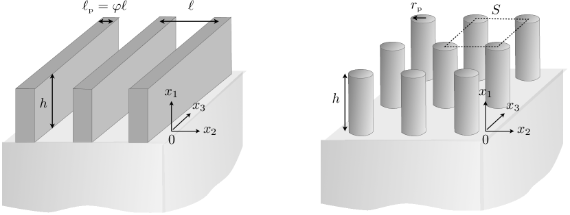
(a)                                                                     (b)

Figure 1: Geometry of the actual problems: (a) Array of parallel plates infinite along $x_{3}$ atop an isotropic substrate; (b) Doubly periodic array of cylindrical beams atop an isotropic substrate. The scalings are chosen to capture the bending resonances only; with $k_{\text{\tiny T}}$ the wavenumber in the substrate, $k_{\text{\tiny T}}h=\eta$ and $k_{\text{\tiny T}}\ell=O(\eta^{2})$.

In this study, we use asymptotic analysis and homogenization techniques to revisit the problem of the interaction of a periodic array of plates or beams on the propagation of seismic waves in three dimensions. We consider slender bodies in the low frequency limit which means two things. Firstly, the typical wavelength $1/k$ is much larger than the array spacing $\ell$, which is a classical hypothesis. Secondly, we focus on the lowest resonances of the bodies being flexural resonances. The first flexural resonances correspond to $kh\sim\ell_{\text{\tiny p}}/h$, with $\ell_{\text{\tiny p}}$ the body thickness, $h$ the body height and $\ell_{\text{\tiny p}}/h$ the slenderness (in comparison the first longitudinal resonance appears at $kh\sim 1$). Now, we consider dense arrays, which means that $\ell_{\text{\tiny p}}\sim\ell$, and $\varphi=\ell_{\text{\tiny p}}/\ell\in(0,1)$ (Figure 1). Hence the asymptotic analysis is conducted considering that

the wavelength $$1/k h \ell_{\text{\tiny p}}\sim\ell$$ is large compared to which is itself large compared to .

It is worth noting that assuming $\varphi=O(\eta^{n})$ with $n\geq 1$ would allow a reduction of model in a first step, resulting in concentrated force problems, as implicitly considered in [19, 21, 35]. Here on the contrary, the implementation of the asymptotic method will require that we reconstruct the asymptotic theory of plates and beams in a low frequency regime, as previously done for a single body in solid mechanics, see e.g. [43, 44] for plates and [45, 46, 47, 48] for beams. However, this classical theory has to be complemented with matched asymptotic expansions to link the behavior in the periodic set of bodies with that in the substrate. This “soil-structure” coupling requires a specific treatment as used in interface homogenization [49, 50, 51, 52], see also [53] for a resonant case. In the present case, we shall derive effective boundary and transmission conditions applying in a homogenized region which replaces the actual array; and in this effective region the wave equation for flexural waves applies. This problem can be further simplified in effective boundary conditions of the Robin type applying on the surface of the soil, namely

$${\bm{\sigma}}\cdot{\bf n}={\mathsf{K}}(\omega){\bf u},$$ (1)

where the frequency-dependent rigidity matrix ${\mathsf{K}}$ depends explicitly on the flexural frequencies of the plates/beams. The rigidity matrix is diagonal as soon as the bodies have sufficient symmetry, resulting in effective impedance conditions which ressemble those obtained in [22] in the same settings.

The paper is organized as follows. In §2, we summarize the result of the asymptotic analysis in the case of an array of plates, whose detailed derivation is given in the §3. The resulting ”complete” formulation (3)-(5) is equivalent to that in (6)-(7) thanks to a partial resolution of the problem. In §4, the accuracy of the effective model is inspected by comparison with direct numerics based on multimodal method [54] for an in-plane incident wave. The strong coupling of the array with the ground at the flexural resonances are exemplified and the agreement between the actual and effective problems is discussed. We finish the study in §5 with concluding remarks and perspectives. We provide in the appendix B the effective problem for the an array of beams which is merely identical to the case of the plates with some specificities which are addressed.

2 The actual problem and the effective problem

We consider in this section the asymptotic analysis of an array of parallel plates atop an isotropic elastic substrate. We note that the problem splits in the in-plane and out-of-plane polarizations. The latter case has been already addressed in [36]. We focus in this section on the former, in-plane, case. We further note that the asymptotic analysis of a doubly periodic array of cylinders atop an isotropic substrate is a fully coupled elastodynamic wave problem, which is thus slightly more involved and addressed in the Appendix.

2.1 The physical problem

We consider the equation of elastodynamics for the displacement vector ${\bf u}$ the stress tensor ${\bm{\sigma}}$ and the strain tensor ${\bm{\varepsilon}}$

$$\left\{\begin{array}[]{ll}\text{in the substrate},x_{1}\in(-\infty,0):&\text{div}{\bm{\sigma}}+\rho_{\text{\tiny s}}\omega^{2}{\bf u}={\bf 0},\quad{\bm{\sigma}}=2\mu_{\text{\tiny s}}{\bm{\varepsilon}}+\lambda_{\text{\tiny s}}\text{tr}({\bm{\varepsilon}}){\mathsf{\bm{missing}}I},\quad{\bm{\varepsilon}}=\frac{1}{2}(\nabla{\bf u}+\;^{t}\nabla{\bf u}),\\[10.0pt] \text{in the plates},x_{1}\in(0,\ell):&\text{div}{\bm{\sigma}}+\rho_{\text{\tiny p}}\omega^{2}{\bf u}={\bf 0},\quad{\bm{\sigma}}=2\mu_{\text{\tiny p}}{\bm{\varepsilon}}+\lambda_{\text{\tiny p}}\text{tr}({\bm{\varepsilon}}){\mathsf{\bm{missing}}I},\end{array}\right.$$ (2)

with the Lamé coefficients $(\lambda_{\text{\tiny p}},\mu_{\text{\tiny p}})$ of the plates and $(\lambda_{\text{\tiny s}},\mu_{\text{\tiny s}})$ of the substrate, $\omega$ the angular frequency and ${\mathsf{\bm{missing}}I}$ stands for the identity matrix. In three dimensions with ${\bf x}=(x_{1},x_{2},x_{3})$, stress free conditions ${\bm{\sigma}}\cdot{\bf n}={\bf 0}$ apply at each boundary between an elastic medium (the plates or the substrate) and air, with $\bf n$ the normal to the interface. Eventually, the continuity of the displacement and the normal stress apply at each boundary between the parallel plates and the substrate. This problem can be solved once the source ${\bf u}^{\text{\tiny inc}}$ has been defined and accounting for the radiation condition for $x_{1}\to-\infty$ which applies to the scattered field $({\bf u}-{\bf u}^{\text{\tiny inc}})$.

2.2 The effective problem

Below we summarize the main results of the analysis developed in the §3 and which provides the so-called ”complete formulation” where the array of parallel plates is replaced by an equivalent layer associated to effective boundary and transmission conditions (Figure 2(a)). Owing to a partial resolution, this formulation can be simplified to an equivalent ”impedance formulation” set on the substrate only (Figure 2(b)). We note that all three components of the displacement field appear in this section, and the reader should be aware that we make use of variables ${\bf x}=(x_{1},x_{2},x_{3})$ and ${\bf x}^{\prime}=(x_{2},x_{3})$.

2.2.1 Complete formulation

The effective problem reads as follow

$$\left\{\begin{array}[]{ll}\displaystyle\text{In the substrate},x_{1}\in(-\infty,0):&\text{div}{\bm{\sigma}}+\rho_{\text{\tiny s}}\omega^{2}{\bf u}={\bf 0},\quad{\bm{\sigma}}=2\mu_{\text{\tiny s}}{\bm{\varepsilon}}+\lambda_{\text{\tiny s}}\text{tr}({\bm{\varepsilon}}){\mathsf{\bm{missing}}I},\\[12.0pt] \displaystyle\text{In the region of the plates},x_{1}\in(0,h):&\displaystyle\frac{\partial^{4}u_{2}}{\partial x_{1}^{4}}-\kappa^{4}\,u_{2}=0,\quad\kappa=\left(\frac{\rho_{\text{\tiny p}}\omega^{2}\ell_{\text{\tiny p}}}{D_{\text{\tiny p}}}\right)^{1/4},\\[10.0pt] &u_{1}(x_{1},{\bf x}^{\prime})=u_{1}(0,{\bf x}^{\prime}),\quad u_{3}(x_{1},{\bf x}^{\prime})=u_{3}(0,{\bf x}^{\prime}),\end{array}\right.$$ (3)

with ${\bf x}^{\prime}=(x_{2},x_{3})$,

$$D_{\text{\tiny p}}=\frac{E_{\text{\tiny p}}}{(1-\nu_{\text{\tiny p}}^{2})}\frac{\ell_{\text{\tiny p}}^{3}}{12},$$ (4)

the flexural rigidity of the plates ($\rho_{\text{\tiny p}}$ the mass density, $E_{\text{\tiny p}}$ the Young’s modulus and $\nu_{\text{\tiny p}}$ the Poisson’s ratio), complemented with boundary conditions at $x_{1}=0$ and $x_{1}=h$ of the form

$$\left\{\begin{array}[]{l}\displaystyle\sigma_{11}(0^{-},{\bf x}^{\prime})=\rho_{\text{\tiny p}}\omega^{2}\varphi h\;u_{1}(0,{\bf x}^{\prime}),\quad\displaystyle\sigma_{12}(0^{-},{\bf x}^{\prime})=-\frac{D_{\text{\tiny p}}}{\ell}\,\;\frac{\partial^{3}u_{2}}{\partial x_{1}^{3}}(0^{+},{\bf x}^{\prime}),\\[10.0pt] \displaystyle\sigma_{13}(0^{-},{\bf x}^{\prime})=\varphi h\left(E_{\text{\tiny p}}\frac{\partial^{2}u_{3}}{\partial x_{3}^{2}}(0^{-},{\bf x}^{\prime})+\rho_{\text{\tiny p}}\omega^{2}u_{3}(0^{-},{\bf x}^{\prime})\right),\\[10.0pt] \displaystyle{u_{2}}(0^{+},{\bf x}^{\prime})={u_{2}}(0^{-},{\bf x}^{\prime}),\quad\displaystyle\frac{\partial u_{2}}{\partial x_{1}}(0^{+},{\bf x}^{\prime})=0,\\[10.0pt] \displaystyle\frac{\partial^{2}u_{2}}{\partial x_{1}^{2}}(h,{\bf x}^{\prime})=\frac{\partial^{3}u_{2}}{\partial x_{1}^{3}}(h,{\bf x}^{\prime})=0.\end{array}\right.$$ (5)

These effective conditions express (i) at $x_{1}=0$ a balance of the stress, prescribed displacements and vanishing rotation and (ii) at $x_{1}=h$, free end conditions with vanishing bending moment and shearing force. One notes that all three components of the displacement field ${\bf u}$ appear in (5) which involves partial derivatives on $x_{1}$ and $x_{3}$ only.

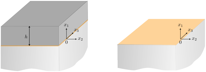
(a)                                                                     (b)

Figure 2: Geometry in the effective problems for an array of plates. (a) In the complete formulation, the region of the array is replaced by an equivalent layer where (3) applies, complemented by the transmission conditions in (5). (b) In the impedance formulation, the problem is reduced to effective boundary conditions (6) which hold at $x_{1}=0$. The same holds for the array of beams, with (a) (55)-(57) and (b) (59).

2.2.2 Impedance formulation

From (3), the problem in $x_{1}\in(0,h)$ can be solved owing to the linearity of the problem with respect to $u_{2}(0^{-},x_{2})$, see A. Doing so, the problem can be thought in the substrate only along with the boundary conditions of the Robin’s type, namely

$$\left\{\begin{array}[]{l}\displaystyle\text{div}{\bm{\sigma}}+\rho_{\text{\tiny s}}\omega^{2}{\bf u}={\bf 0},\quad{\bm{\sigma}}=2\mu_{\text{\tiny s}}{\bm{\varepsilon}}+\lambda_{\text{\tiny s}}\text{tr}({\bm{\varepsilon}}){\mathsf{\bm{missing}}I},\quad x_{1}\in(-\infty,0),\\[12.0pt] \displaystyle\sigma_{11}(0,{\bf x}^{\prime})=\;Z\,u_{1}(0,{\bf x}^{\prime}),\quad\displaystyle\sigma_{12}(0,{\bf x}^{\prime})=Z\;f(\kappa h)\;u_{2}(0,{\bf x}^{\prime}),\\[10.0pt] \displaystyle\sigma_{13}(0,{\bf x}^{\prime})=\varphi h\left(E_{\text{\tiny p}}\frac{\partial^{2}u_{3}}{\partial x_{3}^{2}}(0,{\bf x}^{\prime})+\rho_{\text{\tiny p}}\omega^{2}u_{3}(0,{\bf x}^{\prime})\right),\end{array}\right.$$ (6)

with the following impedance parameters

$$Z=\rho_{\text{\tiny p}}\omega^{2}\varphi h,\quad f(\kappa h)=\frac{\text{sh}\kappa h\cos\kappa h+\text{ch}\kappa h\sin\kappa h}{\kappa h(1+\text{ch}\kappa h\cos\kappa h)},$$ (7)

(we have used that $D_{\text{\tiny p}}\kappa^{4}=\rho_{\text{\tiny p}}\omega^{2}\ell_{\text{\tiny p}}$). The conditions on $(\sigma_{11},\sigma_{12})$ encapsulate the effects of the in-plane bending of the plates while the condition on $\sigma_{13}$ can be understood as the equilibrium of an axially loaded bar (in the absence of substrate, we recover the wave equation for quasi-longitudinal waves). It is worth noting that for out-of-plane displacements, $u_{3}(x_{1},x_{2})$ and $u_{1}=u_{2}=0$, the boundary conditions simplify to $\sigma_{13}(0,x_{2})=\rho_{\text{\tiny p}}\varphi h\omega^{2}u_{3}(0,x_{2})$. This corresponds to the impedance condition which can be deduced from the analysis conducted in [36] and resulting in $\sigma_{13}(0,x_{2})=\mu_{\text{\tiny p}}\varphi k_{\text{\tiny T}}\tan(k_{\text{\tiny T}}h)u_{3}(0,x_{2})$ and obtained here in the limit $k_{\text{\tiny T}}h\ll 1$.

3 Derivation of the effective problem

As previously said, the asymptotic analysis is conducted considering that the typical wavelength $1/k$ is large compared to the plate height $h$ which is itself large compared to the array spacing $\ell\sim\ell_{\text{\tiny p}}$. Hence, with $k_{\text{\tiny T}}=\omega\sqrt{\rho_{\text{\tiny s}}/\mu_{\text{\tiny s}}}$ and $k_{\text{\tiny L}}=\omega\sqrt{\rho_{\text{\tiny s}}/(\lambda_{\text{\tiny s}}+2\mu_{\text{\tiny s}})}$ of the same order of magnitude, we define the small non-dimensional parameter $\eta$ as

$$\eta=\sqrt{k_{\text{\tiny T}}\ell},\quad\text{and}\quad k_{\text{\tiny T}}h=O(\eta),$$

(note that to excite both the bending and the longitudinal modes another scaling is required with $kh=O(1)$, and this is a higher frequency regime studied in [35]). Accordingly, the asymptotic analysis is conducted using the rescaled height $\hat{h}$ of the plates and array’s spacing $\hat{\ell}$ defined by

$$(\hat{h},\hat{\ell})=\left(\frac{h}{\eta},\frac{\ell}{\eta^{2}}\right),$$

which models an array of densely packed thin plates. We also define the associated rescaled spatial coordinates

$$y_{1}=\frac{x_{1}}{\eta},\quad{\bf z}=\frac{{\bf x}}{\eta^{2}}.$$ (8)

3.1 Effective wave equation in the region of the plates

3.1.1 Notations

In the region of the array of parallel plates, the displacements and the stresses vary in the horizontal direction over small distances dictated by $\ell$, and over large distances dictated by the incoming waves; these two scales are accounted for by the two-scale coordinates $({\bf x}^{\prime},z_{2})$, with ${\bf x}^{\prime}=(x_{2},x_{3})$. In the vertical direction, the variations are dictated by $h$ only and this is accounted for by the rescaled coordinate $y_{1}$. It follows that the fields $({\bf u},{\bm{\sigma}})$ are written of the form

$${\bf u}=\sum_{n\geq 0}\eta^{n}{\bf w}^{n}(y_{1},z_{2},{\bf x}^{\prime}),\quad{\bm{\sigma}}=\sum_{n\geq 0}\eta^{n}{\bm{\pi}}^{n}(y_{1},z_{2},{\bf x}^{\prime}),$$ (9)

with the three-scale differential operator reading

$$\nabla\to\frac{{\bm{e}}_{1}}{\eta}\frac{\partial}{\partial y_{1}}+\frac{{\bm{e}}_{2}}{\eta^{2}}\,\frac{\partial}{\partial z_{2}}+\nabla_{{\bf x}^{\prime}},$$ (10)

where ${\bm{e}}_{1}=(1,0,0)$ and ${\bm{e}}_{2}=(0,1,0)$. Now, we introduce the strain tensor with respect to ${\bf x}^{\prime}$

$${\bm{\varepsilon}}^{{\bf x}^{\prime}}({\bf u})=\frac{1}{2}\begin{pmatrix}0&\displaystyle\partial_{x_{2}}{u_{1}}&\partial_{x_{3}}{u_{1}}\\[8.0pt] \partial_{x_{2}}{u_{1}}&2\partial_{x_{2}}{u_{2}}&\left(\partial_{x_{3}}{u_{2}}+\partial_{x_{2}}{u_{3}}\right)\\[8.0pt] \partial_{x_{3}}{u_{1}}&\left(\partial_{x_{3}}{u_{2}}+\partial_{x_{2}}{u_{3}}\right)&2\partial_{x_{3}}{u_{3}}\end{pmatrix},$$ (11)

and the strain tensors with respect to the rescaled coordinates $y_{1}$ and $z_{2}$,

$${\bm{\varepsilon}}^{y_{1}}({\bf u})=\frac{1}{2}\begin{pmatrix}2\partial_{y_{1}}{w_{1}}&\partial_{y_{1}}{u_{2}}&\partial_{y_{1}}{u_{3}}\\[8.0pt] \partial_{y_{1}}{u_{2}}&0&0\\[8.0pt] \partial_{y_{1}}{u_{3}}&0&0\end{pmatrix},\quad{\bm{\varepsilon}}^{z_{2}}({\bf u})=\frac{1}{2}\begin{pmatrix}0&\partial_{z_{2}}{u_{1}}&0\\[8.0pt] \partial_{z_{2}}{u_{1}}&2\partial_{z_{2}}{u_{2}}&\partial_{z_{2}}{u_{3}}\\[8.0pt] 0&\partial_{z_{2}}{u_{3}}&0\end{pmatrix}.$$ (12)

The system in the region of the plates reads, from (2),

$$\left\{\begin{array}[]{ll}(\text{E}_{1})\quad\displaystyle\frac{1}{\eta}\partial_{y_{1}}{\sigma_{11}}+\partial_{x_{\alpha}}{\sigma_{1\alpha}}+\frac{1}{\eta^{2}}\,\partial_{z_{2}}{\sigma_{12}}+\rho_{\text{\tiny p}}\omega^{2}u_{1}=0,\\[10.0pt] (\text{E}_{\alpha})\quad\displaystyle\frac{1}{\eta}\partial_{y_{1}}{\sigma_{\alpha 1}}+\partial_{x_{\beta}}{\sigma_{\alpha\beta}}+\frac{1}{\eta^{2}}\,\partial_{z_{2}}{\sigma_{\alpha 2}}+\rho_{\text{\tiny p}}\omega^{2}u_{\alpha}=0,\\[10.0pt] (\text{C})\quad\displaystyle{\bm{\sigma}}=\frac{1}{\eta}\left(2\mu_{\text{\tiny p}}{\bm{\varepsilon}}^{y_{1}}+\lambda_{\text{\tiny p}}\text{tr}({\bm{\varepsilon}}^{y_{1}})\right)+\left(2\mu_{\text{\tiny p}}{\bm{\varepsilon}}^{{\bf x}^{\prime}}+\lambda_{\text{\tiny p}}\text{tr}({\bm{\varepsilon}}^{{\bf x}^{\prime}})\right)+\frac{1}{\eta^{2}}\left(2\mu_{\text{\tiny p}}{\bm{\varepsilon}}^{{\bf z}^{\prime}}+\lambda_{\text{\tiny p}}\text{tr}({\bm{\varepsilon}}^{{\bf z}^{\prime}})\right),\\[10.0pt] \end{array}\right.$$ (13)

with the convention on the Greek letters $\alpha=2,3$, the same for $\beta$, and where ${\bm{\varepsilon}}$ stands for ${\bm{\varepsilon}}({\bf u})$.

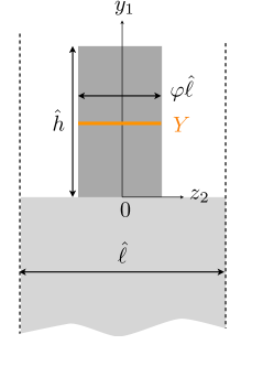
Figure 3: Analysis of a single plate in rescale coordinates, (9) with $Y=\{z_{2}\in(-\varphi\hat{\ell}/2,\varphi\hat{\ell}/2)\}$; the analysis holds within the plate far from its boundaries at $y_{1}=0,\hat{h}$.

We shall use the stress-strain relation written in the form

$$(\text{C}^{\prime})\quad\displaystyle\frac{1}{\eta}{\bm{\varepsilon}}^{y_{1}}+{\bm{\varepsilon}}^{{\bf x}^{\prime}}+\frac{1}{\eta^{2}}\,{\bm{\varepsilon}}^{z_{2}}=\frac{(1+\nu_{\text{\tiny p}})}{E_{\text{\tiny p}}}\,{\bm{\sigma}}-\frac{\nu_{\text{\tiny p}}}{E_{\text{\tiny p}}}\,\text{tr}({\bm{\sigma}})\,{\mathsf{\bm{missing}}I}.$$ (14)

Eventually, the boundary conditions read

$${\sigma_{2i}}=0,\quad i=1,2,3,\quad{at}\;z_{2}=\pm\varphi\hat{\ell}/2,$$ (15)

and are complemented by boundary conditions at $y_{1}=0,\hat{h}$ assumed to be known (they will be justified later). We seek to establish the effective behaviour in the region of the array in terms of macroscopic averaged fields which do not depend anymore on the rapid coordinate $z_{2}$ associated with the small scale $\hat{\ell}$ as the following averages taken along rescaled variable $z_{2}$. These fields are defined at any order $n$ as

$$\overline{{\bf w}^{n}}(y_{1},{\bf x}^{\prime})=\frac{1}{\varphi\hat{\ell}}\int_{Y}{\bf w}^{n}(y_{1},z_{2},{\bf x}^{\prime})\,{\text{d}}z_{2},\quad\overline{{\bm{\pi}}^{n}}(y_{1},{\bf x}^{\prime})=\frac{1}{\hat{\ell}}\int_{Y}{\bm{\pi}}^{n}(y_{1},z_{2},{\bf x}^{\prime})\,{\text{d}}z_{2},$$

with $Y=\{z_{2}\in(-\varphi\hat{\ell}/2,\varphi\hat{\ell}/2)\}$ the segment shown in figure 3.

3.1.2 Sequence of resolution and main results of the analysis

We shall derive the equation satisfied in the region of the array, and additional results on the stresses $(\overline{\pi^{0}_{1i}},\overline{\pi^{1}_{1i}}\,)$, $i=1,2,3$, required to establish the effective boundary conditions at $y_{1}=0,\hat{h}$. The main results will be obtained following the procedure :

1. We establish the following properties on ${\bm{\pi}}^{0}$

   $$\overline{\pi^{0}_{11}}=0,\quad\pi^{0}_{2i}=0,\;i=1,2,3,\quad\overline{\pi_{13}^{0}}=0.$$ (16)

2. Then we derive the dependence of $({\bf w}^{0},{\bf w}^{1})$ on $z_{2}$ which have the form

   $$\left\{\begin{array}[]{l}w^{0}_{1}=W^{0}_{1}({\bf x}^{\prime}),\quad w^{0}_{2}=W^{0}_{2}(y_{1},{\bf x}^{\prime}),\quad w^{0}_{3}=W^{0}_{3}({\bf x}^{\prime}),\\[10.0pt] \displaystyle w^{1}_{1}=W_{1}^{1}({\bf x}^{\prime})-\frac{\lambda_{\text{\tiny p}}}{2(\lambda_{\text{\tiny p}}+\mu_{\text{\tiny p}})}\frac{\partial W_{3}^{0}}{\partial x_{3}}({\bf x}^{\prime})\,y_{1}-\frac{\partial W^{0}_{2}}{\partial y_{1}}(y_{1},{\bf x}^{\prime})\,z_{2},\quad w^{1}_{\alpha}=W^{1}_{\alpha}(y_{1},{\bf x}^{\prime}),\\ \end{array}\right.$$ (17)

   and

   $$\pi_{11}^{0}=-\frac{E_{\text{\tiny p}}}{1-\nu_{\text{\tiny p}}^{2}}\frac{\partial^{2}W^{0}_{2}}{\partial y_{1}^{2}}(y_{1},{\bf x}^{\prime})\;z_{2},\quad\displaystyle\overline{\pi_{33}^{0}}=\varphi E_{\text{\tiny p}}\frac{\partial W_{3}^{0}}{\partial x_{3}}({\bf x}^{\prime}).$$ (18)

3. Eventually, we identify the form of $\overline{\pi^{1}_{1i}}$, $i=1,2,3$, and the Euler -Bernoulli equation governing the bending $W^{0}_{2}$. Specifically

   $$\left\{\begin{array}[]{l}\displaystyle\overline{\pi_{11}^{1}}(y_{1},{\bf x}^{\prime})=\rho_{\text{\tiny p}}\omega^{2}\varphi\,W_{1}^{0}({\bf x}^{\prime})\,(\hat{h}-y_{1}),\\[12.0pt] \displaystyle\overline{\pi^{1}_{12}}(y_{1},{\bf x}^{\prime})=-\frac{E_{\text{\tiny p}}}{(1-\nu_{\text{\tiny p}}^{2})}\frac{\varphi^{3}\hat{\ell}^{2}}{12}\frac{\partial^{3}W_{2}^{0}}{\partial y_{1}^{3}}(y_{1},{\bf x}^{\prime}),\\[12.0pt] \displaystyle\overline{\pi^{1}_{13}}(y_{1},{\bf x}^{\prime})=\varphi\left(E_{\text{\tiny p}}\frac{\partial^{2}W^{0}_{3}}{\partial x_{3}^{2}}({\bf x}^{\prime})+\rho_{\text{\tiny p}}\omega^{2}W^{0}_{3}({\bf x}^{\prime})\right)\left(\hat{h}-y_{1}\right),\end{array}\right.$$ (19)

   and

   $$\frac{E_{\text{\tiny p}}}{(1-\nu_{\text{\tiny p}}^{2})}\,\frac{\varphi^{2}\hat{\ell}^{2}}{12}\,\frac{\partial^{4}W^{0}_{2}}{\partial y_{1}^{4}}-\rho_{\text{\tiny p}}\omega^{2}\,W^{0}_{2}=0.$$ (20)

In the remainder of this section, we shall establish the above results. We shall denote $(\text{E}_{1})^{n}$, $(\text{E}_{\alpha})^{n}$ and $(\text{C})^{n}$ the equations which correspond to terms in (13) factor of $\eta^{n}$.

3.1.3 First step: properties of $\bf\pi^{0}$ in (16)

From $(\text{E})^{-2}$ in (13), we have that $\partial_{z_{2}}{\pi^{0}_{2i}}=0$, which along with the boundary conditions at $z_{2}=\pm\varphi\hat{h}/2$ leave us with $\pi^{0}_{2i}=0$. Next from $(\text{E}_{1})^{-1}$ and $(\text{E}_{3})^{-1}$, we also have that $\partial_{y_{1}}{\pi^{0}_{11}}+\partial_{z_{2}}{\pi^{1}_{12}}=0$ and $\partial_{y_{1}}{\pi^{0}_{13}}+\partial_{z_{2}}{\pi^{1}_{23}}=0$; by averaging these relations over $Y$ and accounting for ${\pi^{1}_{2i}}_{|{\,\partial Y}}=0$, we get that $\overline{\pi^{0}_{11}}$ and $\overline{\pi^{0}_{13}}$ do not depend on $y_{1}$. We now anticipate the boundary condition $\overline{\pi^{0}_{11}}(\hat{h},{\bf x}^{\prime})=\overline{\pi^{0}_{13}}(\hat{h},{\bf x}^{\prime})=0$ that we shall prove later on (see forthcoming (35)), we get $\overline{\pi^{0}_{11}}=\overline{\pi^{0}_{13}}=0$ in $Y$. We have the properties announced in (16).

3.1.4 Second step: $({\bf w}^{0},{\bf w}^{1})$ in (17) and $(\pi^{0}_{11},\overline{\pi_{33}^{0}}\,)$ in (18)

Some of the announced results are trivially obtained. From $(\text{C}^{\prime})^{-2}$ in (14), we get that $\partial_{z_{2}}{w^{0}_{i}}=0$, and from $(\text{C}^{\prime}_{11})^{-1}$ and $(\text{C}^{\prime}_{13})^{-1}$ that $\partial_{y_{1}}{w^{0}_{1}}=\partial_{y_{1}}{w^{0}_{3}}=0$, which leaves us with the form of ${\bf w}^{0}$ in (17). Next $(\text{C}^{\prime}_{\alpha\alpha})^{-1}$ tells us that $\partial_{z_{2}}{w^{1}_{\alpha}}=0$, in agreement with the form of $w_{\alpha}^{1}$ in (17). We have yet to derive the form of $w_{1}^{1}$, which is more demanding. From $(\text{C}^{\prime}_{12})^{-1}$, $\partial_{z_{2}}{w^{1}_{1}}=-\partial_{y_{1}}{w_{2}^{0}}$ and thus

$$w^{1}_{1}=W_{1}(y_{1},{\bf x}^{\prime})-\frac{\partial W^{0}_{2}}{\partial y_{1}}(y_{1},{\bf x}^{\prime})\,z_{2},$$ (21)

but we can say more on $W_{1}$. Let us consider the system provided by $(\text{C}_{11})^{0}$ and $(\text{C}_{22})^{0}$, specifically

$$\left\{\begin{array}[]{ll}\pi^{0}_{11}=&\displaystyle(\lambda_{\text{\tiny p}}+2\mu_{\text{\tiny p}})\partial_{y_{1}}{w_{1}^{1}}+\lambda_{\text{\tiny p}}\left(\partial_{x_{\alpha}}{w^{0}_{\alpha}}+\partial_{z_{2}}{w^{2}_{2}}\right),\\ 0=&\displaystyle(\lambda_{\text{\tiny p}}+2\mu_{\text{\tiny p}})\left(\partial_{z_{2}}{w_{2}^{2}}+\partial_{x_{2}}{w_{2}^{0}}\right)+\lambda_{\text{\tiny p}}\left(\partial_{y_{1}}{w^{1}_{1}}+\partial_{x_{3}}{w^{0}_{3}}\right),\end{array}\right.$$ (22)

where we have used that $\pi_{22}^{0}=0$. After elimination of $\partial_{z_{2}}{w_{2}^{2}}$ and owing to the form of $w^{0}_{\alpha}$ in (16) and $w^{1}_{1}$ in (21) (at this stage), we get $\pi^{0}_{11}=a(y_{1},{\bf x}^{\prime})z_{2}+b(y_{1},{\bf x}^{\prime})$ with

$$a=-\frac{E_{\text{\tiny p}}}{1-\nu_{\text{\tiny p}}^{2}}\frac{\partial^{2}W^{0}_{2}}{\partial y_{1}^{2}}(y_{1},{\bf x}^{\prime}),\quad b=\frac{2\mu_{\text{\tiny p}}}{(\lambda_{\text{\tiny p}}+2\mu_{\text{\tiny p}})}\left(2(\lambda_{\text{\tiny p}}+\mu_{\text{\tiny p}})\frac{\partial W_{1}}{\partial y_{1}}(y_{1},{\bf x}^{\prime})+\lambda_{\text{\tiny p}}\frac{\partial W_{3}^{0}}{\partial x_{3}}({\bf x}^{\prime})\right),$$ (23)

(we have used that ${E_{\text{\tiny p}}}/(1-\nu_{\text{\tiny p}}^{2})=4\mu_{\text{\tiny p}}(\mu_{\text{\tiny p}}+\lambda_{\text{\tiny p}})/(\lambda_{\text{\tiny p}}+2\mu_{\text{\tiny p}})$). It is now sufficient to remark that $\overline{\pi_{11}^{0}}=0$ imposes $b=0$. This immediately provides the form of $\pi^{0}_{11}$ in (18) and

$$W_{1}(y_{1},{\bf x}^{\prime})=W_{1}^{1}({\bf x}^{\prime})-\frac{\lambda_{\text{\tiny p}}}{2(\lambda_{\text{\tiny p}}+\mu_{\text{\tiny p}})}\frac{\partial W_{3}^{0}}{\partial x_{3}}({\bf x}^{\prime})\,y_{1},$$ (24)

which along with (21) leaves us with the form of $w_{1}^{1}$ in (17). The same procedure is used to get $\pi_{33}^{0}$, which from $(\text{C}_{33})^{0}$, reads

$$\pi^{0}_{33}=\displaystyle(\lambda_{\text{\tiny p}}+2\mu_{\text{\tiny p}})\partial_{x_{3}}{w_{3}^{0}}+\lambda_{\text{\tiny p}}\left(\partial_{y_{1}}{w^{1}_{1}}+\partial_{x_{2}}{w^{0}_{2}}+\partial_{z_{2}}{w^{2}_{2}}\right).$$ (25)

Using that $\pi_{22}^{0}=0$ to eliminate $\partial_{z_{2}}{w^{2}_{2}}$, we get

$$\pi^{0}_{33}=\displaystyle E_{\text{\tiny p}}\frac{\partial W_{3}^{0}}{\partial x_{3}}({\bf x}^{\prime})-\frac{2\mu_{\text{\tiny p}}\lambda_{\text{\tiny p}}}{\lambda_{\text{\tiny p}}+2\mu_{\text{\tiny p}}}\frac{\partial^{2}W_{2}^{0}}{\partial y_{1}^{2}}(y_{1},{\bf x}^{\prime})\,z_{2},$$ (26)

which after integration over $Y$ leaves us with $\overline{\pi^{0}_{33}}$ in (18). Incidentally, $w^{2}_{2}$ can be determined from (22) and we find

$$w^{2}_{2}=-\left(\frac{\partial W_{2}^{0}}{\partial x_{2}}(y_{1},{\bf x}^{\prime})+\frac{\lambda_{\text{\tiny p}}}{2(\lambda_{\text{\tiny p}}+\mu_{\text{\tiny p}})}\,\frac{\partial W^{0}_{3}}{\partial x_{3}}({\bf x}^{\prime})\right)z_{2}+\frac{\lambda_{\text{\tiny p}}}{\lambda_{\text{\tiny p}}+2\mu_{\text{\tiny p}}}\,\frac{\partial^{2}W_{2}^{0}}{\partial y_{1}^{2}}\;\frac{z^{2}_{2}}{2}+W^{2}_{2}(y_{1},{\bf x}^{\prime}).$$ (27)

3.1.5 Third step: the $\overline{\pi^{1}_{1i}}$ in (19) and the Euler-Bernoulli equation in (20).

We start with $(\text{E})^{0}$ in (13) integrated over $Y$, specifically,

$$\frac{\partial\overline{\pi^{1}_{11}}}{\partial y_{1}}+\rho_{\text{\tiny p}}\omega^{2}\varphi\,W_{1}^{0}=0,\quad\displaystyle\frac{\partial\overline{\pi^{1}_{12}}}{\partial y_{1}}+\rho_{\text{\tiny p}}\omega^{2}\varphi\,W_{2}^{0}=0,\quad\displaystyle\frac{\partial\overline{\pi^{1}_{13}}}{\partial y_{1}}+\frac{\partial\overline{\pi^{0}_{33}}}{\partial x_{3}}+\rho_{\text{\tiny p}}\omega^{2}W_{3}^{0}=0,$$ (28)

where we have used (16) and ${\bm{\pi}}^{2}\cdot{\bf n}_{|{\,\partial Y}}={\bf 0}$. Since $W^{0}_{1}$ and $W^{0}_{3}$ depend on ${\bf x}^{\prime}$ only, and accounting for $\overline{\pi^{0}_{33}}({\bf x}^{\prime})$ in (18), we get by integration the forms of $\overline{\pi^{1}_{11}}$ and of $\overline{\pi^{1}_{13}}$ announced in (19). Note that we have anticipated the boundary conditions $\overline{\pi^{1}_{1i}}=0$ at $y_{1}=\hat{h}$, see forthcoming (35).

The equation on $\overline{\pi^{1}_{12}}$ in (28) will provide the Euler-Bernoulli equation once $\overline{\pi^{1}_{12}}$ has been determined (the integration is not possible since $W^{0}_{2}$ depends on $y_{1}$). To do so, we use, that $\partial_{y_{1}}{\pi^{0}_{11}}+\partial_{z_{2}}{\pi^{1}_{12}}=0$, from $(\text{E}_{1})^{-1}$, along with $\pi^{0}_{11}$ in (18). After integration and using the boundary condition of vanishing $\pi^{1}_{12}$ at $z_{2}=\pm\varphi\hat{\ell}/2$, we get that

$$\pi^{1}_{12}=\frac{E_{\text{\tiny p}}}{2(1-\nu_{\text{\tiny p}}^{2})}\frac{\partial^{3}W_{1}^{0}}{\partial y_{1}^{3}}(y_{1},{\bf x}^{\prime})\,\left(z_{2}^{2}-\frac{\varphi^{2}\hat{\ell}^{2}}{4}\right),$$ (29)

hence the form of $\overline{\pi^{1}_{12}}$ in (19). It is now sufficient to use $\pi^{1}_{12}$ in (28) to get the Euler-Bernoulli announced in (20).

3.2 Effective boundary conditions at the top of the array

To derive the transmission conditions at the top of the array, we perform a zoom by substituting $y_{1}$ used in (9) by $z_{1}=y_{1}/\eta$, see Figure 4a. Accordingly, the expansions of the fields are sought of the form

$${\bf u}=\sum_{n\geq 0}\eta^{n}{\bf v}^{n}({\bf z}^{\prime},{\bf x}^{\prime}),\quad{\bm{\sigma}}=\sum_{n\geq 0}\eta^{n}{\bm{\tau}}^{n}({\bf z}^{\prime},{\bf x}^{\prime}),$$ (30)

where we denote ${\bf z}^{\prime}=(z_{1},z_{2})$. The coordinate $z_{1}\in(-\infty,0)$ accounts for small scale variations of the evanescent fields at the top of the plates. Next, the boundary conditions will be obtained by matching the solution in (30) for $z_{1}\to-\infty$ with that in (9) valid far from the boundary for $y_{1}\to\hat{h}$. This means that we ask the two expansions to satisfy

$${\bf v}^{0}(z_{1},z_{2},{\bf x}^{\prime})+\eta{\bf v}^{1}(z_{1},z_{2},{\bf x}^{\prime})+\cdots\underset{z_{1}\to-\infty}{\sim}{\bf w}^{0}(\hat{h}+\eta z_{1},z_{2},{\bf x}^{\prime})+\eta{\bf w}^{1}(\hat{h}+\eta z_{1},z_{2},{\bf x}^{\prime})+\cdots,$$

(and the same for the stress tensors); note that we have used that $y_{1}=\eta z_{1}$. It results that

$$\left\{\begin{array}[]{ll}\displaystyle\lim_{z_{1}\to-\infty}{\bf v}^{0}({\bf z}^{\prime},{\bf x}^{\prime})={\bf w}^{0}(\hat{h},{\bf x}^{\prime}),&\displaystyle\lim_{z_{1}\to-\infty}\left({\bf v}^{1}({\bf z}^{\prime},{\bf x}^{\prime})-z_{1}\frac{\partial{\bf w}^{0}}{\partial y_{1}}(\hat{h},z_{2},{\bf x}^{\prime})\right)={\bf w}^{1}(\hat{h},z_{2},{\bf x}^{\prime}),\\[10.0pt] \displaystyle\lim_{z_{1}\to-\infty}{\bm{\tau}}^{0}({\bf z}^{\prime},{\bf x}^{\prime})={\bm{\pi}}^{0}(\hat{h},z_{2},{\bf x}^{\prime}),&\displaystyle\lim_{z_{1}\to-\infty}\left({\bm{\tau}}^{1}({\bf z}^{\prime},{\bf x}^{\prime})-z_{1}\frac{\partial{\bm{\pi}}^{0}}{\partial y_{1}}(\hat{h},z_{2},{\bf x}^{\prime})\right)={\bm{\pi}}^{1}(\hat{h},z_{2},{\bf x}^{\prime}).\end{array}\right.$$ (31)

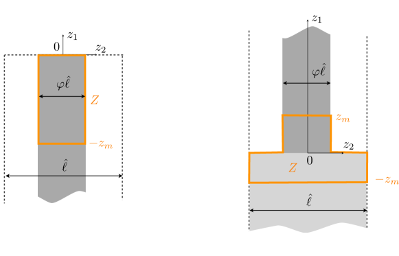
(a)                                                  (b)

Figure 4: Analysis of the effective conditions at the top and at the bottom of the array. (a) Half strip at the top of the array in $(z_{1},z_{2})$ coordinate with $z_{1}\in(-\infty,0)$, (b) Strip at the bottom of the array with $z_{1}\in(-\infty,+\infty)$; for $z_{1}\in(-\infty,0)$, the terms in the expansions (30) are periodic with respect to $z_{2}\in(-\hat{\ell}/2,\hat{\ell}/2)$.

According to the dependence of the fields in (30) on $({\bf z}^{\prime},{\bf x}^{\prime})$, the differential operator reads as follows

$$\nabla\to\frac{1}{\eta^{2}}\,\nabla_{{\bf z}^{\prime}}+\nabla_{{\bf x}^{\prime}},$$ (32)

and we shall need only the first equation of (2), which reads

$$(\text{e})\quad\displaystyle\frac{1}{\eta^{2}}\,\text{div}_{{\bf z}^{\prime}}\,{\bm{\sigma}}+\text{div}_{{\bf x}^{\prime}}{\bm{\sigma}}+\rho_{\text{\tiny p}}\omega^{2}\,{\bf u}={\bf 0},$$ (33)

where $\text{div}_{{\bf z}^{\prime}}$ and $\text{div}_{{\bf x}^{\prime}}$ means the divergence with respect to the coordinate ${\bf z}^{\prime}$ and ${\bf x}^{\prime}$ respectively. In (33), $(\text{e})^{-2}$ and $(\text{e})^{-1}$ tell us that $\text{div}_{{\bf z}^{\prime}}{\bm{\tau}}^{0}=\text{div}_{{\bf z}^{\prime}}{\bm{\tau}}^{1}={\bm{0}}$, that we integrate over $Z=\{z_{1}\in(-z_{m},0),z_{2}\in Y\}$ to get $\int_{\partial Z}{\bm{\tau}}^{0}\cdot{\bf n}\;\text{d}s=\int_{\partial Z}{\bm{\tau}}^{1}\cdot{\bf n}\;\text{d}s={\bf 0}$. On $\partial Z$, ${\bm{\tau}}^{0}\cdot{\bf n}$ and ${\bm{\tau}}^{1}\cdot{\bf n}$ vanish except on the bottom edge $Y$ of $\partial Z$ at $z_{1}=-z_{m}$ where ${\bf n}=-{\bm{e}}_{1}$. It follows, from (31) along with $\overline{\pi^{0}_{1i}}=0$ in (16), that

$${\bf 0}=\lim_{z_{m}\to\infty}\int_{\partial Z}{\bm{\tau}}^{0}\cdot{\bf n}\,\text{d}s=-\hat{\ell}\,\overline{\pi^{0}_{1i}}(\hat{h},{\bf x}^{\prime})\,{\bm{e}}_{i},\quad{\bf 0}=\lim_{z_{m}\to\infty}\int_{\partial Z}{\bm{\tau}}^{1}\cdot{\bf n}\,\text{d}s=-\,\hat{\ell}\overline{\pi^{1}_{1i}}(\hat{h},{\bf x}^{\prime})\,{\bm{e}}_{i}.$$ (34)

which provides the boundary conditions

$$\overline{\pi^{0}_{1i}}(\hat{h},{\bf x}^{\prime})=\overline{\pi^{1}_{1i}}(\hat{h},{\bf x}^{\prime})=0,\quad i=1,2,3.$$ (35)

The conditions on $\overline{\pi^{0}_{1i}}$ are consistent with (16). The conditions on $\overline{\pi^{1}_{11}}$ and $\overline{\pi^{1}_{13}}$ are those anticipated in the previous section, see (19). Eventually, the condition $\overline{\pi^{1}_{12}}(\hat{h},x_{2})=0$ combined with (19) leads to the condition of zero shear force

$$\frac{\partial^{3}W_{2}^{0}}{\partial y_{1}^{3}}(\hat{h},{\bf x}^{\prime})=0.$$ (36)

We have yet to derive the condition of zero bending moment. First, integrating $\text{div}_{\bf z}{\bm{\tau}}^{0}$ over $Z$, we get $0=\int_{\partial Z}\,\tau^{0}_{ij}n_{j}\;\text{d}z_{2}=\int_{Y}\,{\tau^{0}_{12}}_{|{z_{1}=-z_{m}}}\;\text{d}z_{2}$. Next, integrating over $Z$ the scalar ${\bf a}\cdot\text{div}_{\bf z}{\bm{\tau}}^{0}=a_{i}\partial_{z_{j}}{\tau_{ij}^{0}}=0$ (since $\text{div}_{\bf z}{\bm{\tau}}^{0}={\bf 0}$) with ${\bf a}=z_{2}\,{\bm{e}}_{1}-z_{1}{\bm{e}}_{2}$ and integrating by parts, we get that

$$0=\int_{\partial Z}a_{i}\;\tau^{0}_{ij}n_{j}\;\text{d}s=-\int_{Y}\,z_{2}\,{\tau^{0}_{11}}_{|{z_{1}=-z_{m}}}\;\text{d}z_{2}-z_{m}\int_{Y}\,{\tau^{0}_{12}}_{|{z_{1}=-z_{m}}}\;\text{d}z_{2}=-\int_{Y}\,z_{2}\,{\tau^{0}_{11}}_{|{z_{1}=-z_{m}}}\;\text{d}z_{2}.,$$ (37)

(the integral on $\partial Z$ reduces to that on $Y$ at $z=-z_{m}$). In the limit $z_{m}\to\infty$, where $\int_{Y}z_{2}\tau^{0}_{11}\to\overline{z_{2}\pi^{0}_{11}}(\hat{h},{\bf x}^{\prime})$, and accounting for $\pi^{0}_{11}$ in (18), we obtain the expected boundary condition

$$\frac{\partial^{2}W_{2}^{0}}{\partial y_{1}^{2}}(\hat{h},{\bf x}^{\prime})=0.$$ (38)

3.3 Effective transmission conditions between the substrate and the region of the array

To begin with, we shall need the solution in the substrate which is expanded as

$${\bf u}=\sum_{n\geq 0}\eta^{n}{\bf u}^{n}({\bf x}),\quad{\bm{\sigma}}({\bf x})=\sum_{n\geq 0}\eta^{n}{\bm{\sigma}}^{n}({\bf x}),$$ (39)

with no dependence on the rapid coordinates, while in the array it is given by (9). As in the previous section, a zoom is performed in the vicinity of the interface between the substrate and the region of the array, owing to the substitution $y_{1}\to z_{1}$. In the intermediate region, the fields are expanded as in (30) with the interface at $z_{1}=0$ and $z_{1}\in(-\infty,+\infty)$, see Figure 4(b). It is worth noting that for $z_{1}\in(-\infty,0)$ the terms in the expansion (30) are assumed to be periodic with respect to $z_{2}\in(-\hat{\ell}/2,\hat{\ell}/2)$ while for $z_{1}\in(0,\infty)$ we have $z_{2}\in(-\varphi\hat{\ell}/2,\varphi\hat{\ell}/2)$. Note that we should use different notations for the expansions and for $z_{1}$ since their meaning is different; for simplicity, we keep the same. The transmission conditions will be obtained by matching the solution in (30) for $z_{1}\to+\infty$ with that in (9) for $x_{1}\to 0^{+}$, and for $z_{1}\to-\infty$ with that in (39) for $x_{1}\to 0^{-}$. Matching the solutions hence means, with ${\bf z}=(z_{1},z_{2})$,

$$\left\{\begin{array}[]{l}{\bf v}^{0}({\bf z}^{\prime},{\bf x}^{\prime})+\eta{\bf v}^{1}({\bf z}^{\prime},{\bf x}^{\prime})+\cdots\underset{z_{1}\to-\infty}{\sim}{\bf u}^{0}(\eta^{2}z_{1},{\bf x}^{\prime})+\eta{\bf u}^{1}(\eta^{2}z_{1},{\bf x}^{\prime})+\cdots,\\[10.0pt] {\bf v}^{0}({\bf z}^{\prime},{\bf x}^{\prime})+\eta{\bf v}^{1}({\bf z}^{\prime},{\bf x}^{\prime})+\cdots\underset{z_{1}\to+\infty}{\sim}{\bf w}^{0}(\eta z_{1},z_{2},{\bf x}^{\prime})+\eta{\bf w}^{1}(\eta z_{1},z_{2},{\bf x}^{\prime})+\cdots,\end{array}\right.$$

where we have used that $x_{1}=\eta^{2}z_{1}$ and $y_{1}=\eta z_{1}$. It results that

$$\left\{\begin{array}[]{l}\displaystyle\lim_{z_{1}\to-\infty}{\bf v}^{0}({\bf z}^{\prime},{\bf x}^{\prime})={\bf u}^{0}(0^{-},{\bf x}^{\prime}),\quad\lim_{z_{1}\to-\infty}{\bf v}^{1}({\bf z}^{\prime},x_{2})={\bf u}^{1}(0^{-},{\bf x}^{\prime}),\\ \displaystyle\lim_{z_{1}\to-\infty}{\bm{\tau}}^{0}({\bf z}^{\prime},{\bf x}^{\prime})={\bm{\sigma}}^{0}(0^{-},{\bf x}^{\prime}),\quad\lim_{z_{1}\to-\infty}{\bm{\tau}}^{1}({\bf z}^{\prime},{\bf x}^{\prime})={\bm{\sigma}}^{1}(0^{-},{\bf x}^{\prime}),\end{array}\right.$$ (40)

and that

$$\left\{\begin{array}[]{ll}\displaystyle\lim_{z_{1}\to+\infty}{\bf v}^{0}({\bf z}^{\prime},{\bf x}^{\prime})={\bf w}^{0}(0^{+},{\bf x}^{\prime}),&\displaystyle\lim_{z_{1}\to+\infty}\left({\bf v}^{1}({\bf z}^{\prime},{\bf x}^{\prime})-z_{1}\frac{\partial{\bf w}^{0}}{\partial y_{1}}(0^{+},z_{2},{\bf x}^{\prime})\right)={\bf w}^{1}(0^{+},z_{2},{\bf x}^{\prime}),\\[10.0pt] \displaystyle\lim_{z_{1}\to+\infty}{\bm{\tau}}^{0}({\bf z}^{\prime},{\bf x}^{\prime})={\bm{\pi}}^{0}(0^{+},z_{2},{\bf x}^{\prime}),&\displaystyle\lim_{z_{1}\to+\infty}\left({\bm{\tau}}^{1}({\bf z}^{\prime},{\bf x}^{\prime})-z_{1}\frac{\partial{\bm{\pi}}^{0}}{\partial y_{1}}(0^{+},z_{2},{\bf x}^{\prime})\right)={\bm{\pi}}^{1}(0^{+},z_{2},{\bf x}^{\prime}).\end{array}\right.$$ (41)

Eventually, with the differential operator in (32), (33) applies; we shall also need from (2) that

$$(\text{c})\quad\eta^{2}{\bm{\sigma}}=2\mu_{\text{\tiny a}}\,{\bm{\varepsilon}}^{{\bf z}^{\prime}}+\lambda_{\text{\tiny a}}\text{tr}({\bm{\varepsilon}}^{{\bf z}^{\prime}}){\mathsf{\bm{missing}}I},\quad\quad(\text{c}^{\prime})\quad\displaystyle\frac{1}{\eta}{\bm{\varepsilon}}^{y_{1}}+{\bm{\varepsilon}}^{{\bf x}^{\prime}}+\frac{1}{\eta^{2}}{\bm{\varepsilon}}^{{\bf z}^{\prime}}=\frac{(1+\nu_{\text{\tiny a}})}{E_{\text{\tiny a}}}\,{\bm{\sigma}}-\frac{\nu_{\text{\tiny a}}}{E_{\text{\tiny a}}}\,\text{tr}({\bm{\sigma}})\,{\mathsf{\bm{missing}}I}.$$ (42)

(${\bm{\varepsilon}}$ stands for ${\bm{\varepsilon}}({\bf u})$) applying in the substrate, a=s, and in the plate, a=p, where we have defined

$${\bm{\varepsilon}}^{{\bf z}^{\prime}}({\bf u})=\frac{1}{2}\begin{pmatrix}2\partial_{z_{1}}{u_{1}}&\left(\partial_{z_{2}}{u_{1}}+\partial_{z_{1}}{u_{2}}\right)&\partial_{z_{1}}{u_{3}}\\[8.0pt] \left(\partial_{z_{2}}{u_{1}}+\partial_{z_{1}}{u_{2}}\right)&2\partial_{z_{2}}{u_{2}}&\partial_{z_{2}}{u_{3}}\\[8.0pt] \partial_{z_{1}}{u_{3}}&\partial_{z_{2}}{u_{3}}&0\end{pmatrix}.$$ (43)

The continuity of the displacement is easily deduced. From $(\text{c}^{\prime})^{-2}$ in (42), $v_{3}^{0}$ does not depend on ${\bf z}^{\prime}$, and $(v_{1}^{0},v_{2}^{0})$ correspond to a rigid body motion, i.e. $v^{0}_{1}=\Omega^{0}_{\text{\tiny a}}z_{2}+{V_{1}^{0}}_{\text{\tiny a}}$ and $v^{0}_{2}=\Omega^{0}_{\text{\tiny a}}z_{1}+{V_{2}^{0}}_{\text{\tiny a}}$, with $(\Omega^{0}_{\text{\tiny a}},{\bf V}^{0}_{\text{\tiny a}})$ independent of ${\bf z}^{\prime}$. The periodic boundary conditions in the substrate impose $\Omega^{0}_{\text{\tiny s}}=0$; next, the continuity of the displacement at $z_{1}=0$ imposes $\Omega^{0}_{\text{\tiny p}}=0$ in the plates and ${\bf v}^{0}={\bf V}^{0}_{\text{\tiny p}}={\bf V}^{0}_{\text{\tiny s}}$ is independent of ${\bf z}^{\prime}$. From (40)-(41), ${\bf u}^{0}(0^{-},{\bf x}^{\prime})={\bf v}^{0}={\bf w}^{0}(0^{+},z_{2},{\bf x}^{\prime})$, and making use of (17)

$$u^{0}_{1}(0^{-},{\bf x}^{\prime})=W_{1}^{0}({\bf x}^{\prime}),\quad u^{0}_{2}(0^{-},{\bf x}^{\prime})=W_{2}^{0}(0^{+},{\bf x}^{\prime}).$$ (44)

For the same reasons, ${\bf v}^{1}$ is a constant displacement, hence ${\bf u}^{1}(0^{-},{\bf x}^{\prime})={\bf w}^{1}(0^{+},z_{2},{\bf x}^{\prime})$, but this has now a consequence. Indeed, from (41) for the displacement at order 1, we have necessarily $\partial_{y_{1}}{{\bf w}^{0}}(0^{+},z_{2},{\bf x}^{\prime})={\bf 0}$ to ensure that ${\bf w}^{1}(0^{+},z_{2},{\bf x}^{\prime})$ is finite; from (17), we already know that $\partial_{y_{1}}{w^{0}_{1}}=\partial_{y_{1}}{w^{0}_{3}}=0$ but the condition remains for $w^{0}_{2}=W^{0}_{2}(y_{1},{\bf x}^{\prime})$, hence

$$\frac{\partial W^{0}_{2}}{\partial y_{1}}(0^{+},{\bf x}^{\prime})=0.$$ (45)

We now move on the effective conditions on the force. From $(\text{c})^{-2}$ in (33), $\text{div}_{{\bf z}^{\prime}}{\bm{\tau}}^{0}={\bf 0}$ that we integrate over $Z=\{z_{1}\in(0,z_{m}),z_{2}\in Y\}\cup\{z_{1}\in(-z_{m},0),z_{2}\in(-\hat{\ell}/2,\hat{\ell}/2)\}$. Accounting for i) ${\bm{\tau}}^{0}\cdot{\bf n}$ continuous at $z_{1}=0$, ii) ${\bm{\tau}}^{0}\cdot{\bf n}=0$ between the plates and the air, iii) ${\bm{\tau}}^{0}$ periodic at $z_{2}=\pm\hat{\ell}/2$ in the substrate, we get that $\int_{-\hat{\ell}/2}^{\hat{\ell}/2}\tau_{1i}^{0}(-z_{m},z_{2},{\bf x}^{\prime})\,{\text{d}}z_{2}=\int_{Y}\tau_{1i}^{0}(z_{m},z_{2},{\bf x}^{\prime})\,{\text{d}}z_{2}$. In the limit $z_{m}\to\infty$ in (40) - (41) along with $\overline{\pi^{0}_{1i}}=0$ from (16), we get

$$\sigma^{0}_{1i}(0^{-},{\bf x}^{\prime})=0,\quad i=1,2,3,$$ (46)

which tells us that the plates do not couple to the substrate at the dominant order. The coupling appears at the next order, starting with $\text{div}_{{\bf z}^{\prime}}{\bm{\tau}}^{1}={\bf 0}$ from $(\text{c})^{-1}$. As for ${\bm{\tau}}^{0}$ and using again that $\overline{\pi^{0}_{1i}}=0$, we get that $\sigma^{1}_{1i}(0^{-},{\bf x}^{\prime})=\overline{\pi^{1}_{1i}}(0^{+},{\bf x}^{\prime})$; eventually, using $\overline{\pi^{1}_{1i}}$ in (19), we get

$$\left\{\begin{array}[]{l}\displaystyle\sigma_{11}^{1}(0^{-},{\bf x}^{\prime})=\rho_{\text{\tiny p}}\omega^{2}\varphi\hat{h}\,W_{1}^{0}({\bf x}^{\prime}),\quad\sigma_{12}^{1}(0^{-},{\bf x}^{\prime})=-\;\frac{E_{\text{\tiny p}}}{(1-\nu_{\text{\tiny p}}^{2})}\,\frac{\varphi^{3}\hat{\ell}^{2}}{12}\,\frac{\partial^{3}W^{0}_{2}}{\partial y_{1}^{3}}(0^{+},{\bf x}^{\prime}),\\ \displaystyle\sigma_{13}^{1}(0^{-},{\bf x}^{\prime})=\varphi\hat{h}\left(E_{\text{\tiny p}}\frac{\partial^{2}W^{0}_{3}}{\partial x_{3}^{2}}({\bf x}^{\prime})+\rho_{\text{\tiny p}}\omega^{2}W^{0}_{3}({\bf x}^{\prime})\right)\end{array}\right.$$ (47)

3.4 The final problem

The effective problem (3) is obtained for $({\bf u}={\bf u}^{0},{\bm{\sigma}}={\bm{\sigma}}^{0}+\eta{\bm{\sigma}}^{1})$ in the substrate for $x_{1}<0$, $({\bf u}={\bf W}^{0},{\bm{\sigma}}={\bm{\pi}}^{0}+\eta{\bm{\pi}}^{1})$ in the region of the array for $x_{1}>0$. Remembering that $y_{1}=x_{1}/\eta$ and $\hat{h}=h/\eta$, $\hat{\ell}=\ell/\eta^{2}$, it is easy to see that (i) the Euler-Bernoulli equation in (3) is obtained from (20), (ii) the effective boundary conditions announced in (5) from (36), (38), (44), (45) and (46)-(47).

4 Numerical validation of the effective problem for a two-dimensional problem

In this section, we inspect the validity of the effective problem in a two-dimensional setting for in-plane waves ($u_{3}=0$, hence $\partial_{x_{3}}=0$). We solve numerically the actual problem of an incident plane wave coming from $x_{1}\to-\infty$ at oblique incidence on the free surface supporting the array of plates, and Lamb waves are excited in the plates. This is done using a multimodal method with pseudo-periodic solutions in the soil and Lamb modes in the plates; the method is detailed in [54]. In the effective problem, the solution is explicit, from (3) - (5) or equivalently (6)-(7) when the solution in the plates is disregarded.

We set the material properties for the elastic substrate: $\nu_{\text{\tiny s}}=0.2$, $E_{\text{\tiny s}}=2$ GPa, $\rho_{\text{\tiny s}}=1000$ Kg.m^-3, and for the plates : $\nu_{\text{\tiny p}}=0.3$, $E_{\text{\tiny p}}=2$ GPa, $\rho_{\text{\tiny p}}=500$ Kg.m^-3, and $\varphi=0.5$. We choose $\ell=1$ m and we set $\eta=\sqrt{k_{\text{\tiny T}}\ell}=0.37$ ($\omega=124$ rad.s^-1), hence $\kappa=0.64$ m^-1. We shall consider $h\in(0,30)$ m resulting in $\kappa h\in(0,20)$ which includes the first 6 bending modes for $h=h_{n}$, $n=1,\cdots,6$, and $h_{1}\simeq 3$ m, $h_{2}\simeq 7.3$ m, $h_{3}\simeq 12.3$ m, $h_{4}=17.2$ m, $h_{5}=22.1$ m, $h_{6}=27.0$ m. The first resonance of the quasi-longitudinal wave along $x_{1}$ appears for $h=\pi/(2\omega)\;\sqrt{E_{\text{\tiny p}}/\rho_{\text{\tiny p}}}\simeq 25.3$ m, hence it will be visible in our results.

4.1 Reflection of elastic waves - the solution of the effective problem

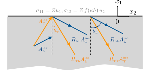
Figure 5: The effective (partial) problem – Reflection of an elastic wave on the surface $x_{1}=0$ where effective boundary conditions (6) apply. The incident wave is defined by (48) and the solution by (49). The arrows show the wavevectors.

We define the potentials $(\phi,\psi)$ using the Helmholtz decomposition, with ${\bf u}=\nabla\phi+\nabla\times(\psi\;{\bf e}_{3})$. The incident wave in the substrate is defined in terms of the incident potentials

$$\left\{\begin{array}[]{l}\displaystyle\phi^{\text{\tiny inc}}(x_{1},x_{2})=A_{\text{\tiny L}}^{\text{\tiny inc}}e^{i\alpha_{\text{\tiny L}}x_{1}}e^{i\beta x_{2}},\quad\psi^{\text{\tiny inc}}(x_{1},x_{2})=A_{\text{\tiny T}}^{\text{\tiny inc}}e^{i\alpha_{\text{\tiny T}}x_{1}}e^{i\beta x_{2}},\\[10.0pt] \displaystyle\text{with }(\alpha_{\text{\tiny L}},\beta)=k_{\text{\tiny L}}\;(\cos\theta_{\text{\tiny L}},\sin\theta_{\text{\tiny L}}),\quad(\alpha_{\text{\tiny T}},\beta)=k_{\text{\tiny T}}\;(\cos\theta_{\text{\tiny T}},\sin\theta_{\text{\tiny T}}),\end{array}\right.$$ (48)

with $k_{\text{\tiny L}}=\sqrt{\frac{\rho_{\text{\tiny s}}}{\lambda_{\text{\tiny s}}+2\mu_{\text{\tiny s}}}}\;\omega$ and $k_{\text{\tiny T}}=\sqrt{\frac{\rho_{\text{\tiny s}}}{\mu_{\text{\tiny s}}}}\;\omega$. The solution in the substrate reads

$$\left\{\begin{array}[]{l}\displaystyle\phi(x_{1},x_{2})=\phi^{\text{\tiny inc}}(x_{1},x_{2})+\left(R_{\text{\tiny LL}}\,A_{\text{\tiny L}}^{\text{\tiny inc}}+R_{\text{\tiny LT}}\,A_{\text{\tiny T}}^{\text{\tiny inc}}\right)e^{-i\alpha_{\text{\tiny L}}x_{1}}e^{i\beta x_{2}},\\[10.0pt] \psi(x_{1},x_{2})=\psi^{\text{\tiny inc}}(x_{1},x_{2})+\left(R_{\text{\tiny TL}}\,A_{\text{\tiny L}}^{\text{\tiny inc}}+R_{\text{\tiny TT}}\,A_{\text{\tiny T}}^{\text{\tiny inc}}\right)e^{-i\alpha_{\text{\tiny T}}x_{1}}e^{i\beta x_{2}}.\end{array}\right.$$ (49)

The effective problem can be solved explicitly. Accounting for the boundary conditions (6), it is easy to show that

$$\left\{\begin{array}[]{l}\displaystyle R_{\text{\tiny LL}}=\frac{1}{D}\;\left[\sin 2\theta_{\text{\tiny T}}\sin 2\theta_{\text{\tiny L}}-\xi^{2}\cos^{2}2\theta_{\text{\tiny T}}-i\xi a\left(\cos\theta_{\text{\tiny L}}-\xi f\cos\theta_{\text{\tiny T}}\right)-\xi a^{2}f\cos(\theta_{\text{\tiny L}}+\theta_{\text{\tiny T}})\right],\\[12.0pt] \displaystyle R_{\text{\tiny TT}}=\frac{1}{D}\;\left[\sin 2\theta_{\text{\tiny T}}\sin 2\theta_{\text{\tiny L}}-\xi^{2}\cos^{2}2\theta_{\text{\tiny T}}+i\xi a\left(\cos\theta_{\text{\tiny L}}-\xi f\cos\theta_{\text{\tiny T}}\right)-\xi a^{2}f\cos(\theta_{\text{\tiny L}}+\theta_{\text{\tiny T}})\right],\\[12.0pt] \displaystyle R_{\text{\tiny LT}}=-\frac{\xi^{2}\sin 2\theta_{\text{\tiny T}}}{D}{\,\left(2\cos 2\theta_{\text{\tiny T}}+a^{2}f\right)},\quad\par\displaystyle R_{\text{\tiny TL}}=\frac{\sin 2\theta_{\text{\tiny L}}}{D}\;{\left(2\cos 2\theta_{\text{\tiny T}}+a^{2}f\right)},\\[10.0pt] \begin{array}[]{ll}\text{where }&\displaystyle D=\sin 2\theta_{\text{\tiny T}}\sin 2\theta_{\text{\tiny L}}+\xi^{2}\cos^{2}2\theta_{\text{\tiny T}}-i\xi a\left(\cos\theta_{\text{\tiny L}}+\xi f\cos\theta_{\text{\tiny T}}\right)-\xi a^{2}f\cos(\theta_{\text{\tiny L}}-\theta_{\text{\tiny T}}),\\[8.0pt] \displaystyle&\displaystyle\text{$f$ stands for $f(\kappa h)$ in \eqref{deff} and }\xi=\frac{\sin\theta_{\text{\tiny L}}}{\sin\theta_{\text{\tiny T}}}=\sqrt{\frac{2(1-\nu_{\text{\tiny s}})}{1-2\nu_{\text{\tiny s}}}},\quad a=\varphi\,\frac{\rho_{\text{\tiny p}}}{\rho_{\text{\tiny s}}}\;k_{\text{\tiny T}}h,\end{array}\end{array}\right.$$ (50)

(note that $a=Z/(k_{\text{\tiny T}}\rho_{\text{\tiny s}})$ in (7)).

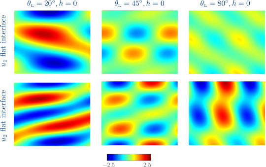
Figure 6: Reference case – Vertical $u_{1}$ and horizontal $u_{2}$ displacement fields in the absence of array. The fields are shown for $x_{1}\in(-100,0)$ m and $x_{2}\in(0,120)$ m.

Obviously, the same reflection coefficients are obtained by solving the complete problem (3)-(5); we get the displacement fields in the region of the plates $x_{1}\in(0,h)$, with

$$\begin{array}[]{c}\displaystyle u_{1}(x_{1},x_{2})=u_{1}(0,x_{2}),\quad{u_{2}}(x_{1},x_{2})=u_{2}(0,x_{2})V(x_{1}),\\[8.0pt] \left\{\begin{array}[]{l}\displaystyle u_{1}(0,x_{2})=\frac{2i\xi^{2}k_{\text{\tiny L}}}{D}\left[\cos\theta_{\text{\tiny L}}\left(\cos 2\theta_{\text{\tiny T}}-i\cos\theta_{\text{\tiny T}}\;af\right)A_{\text{\tiny L}}^{\text{\tiny inc}}+\left(\sin 2\theta_{\text{\tiny T}}\cos\theta_{\text{\tiny L}}-i\sin\theta_{\text{\tiny L}}\cos\theta_{\text{\tiny T}}\;af\right)A_{\text{\tiny T}}^{\text{\tiny inc}}\right]\;e^{i\beta x_{2}},\\[14.0pt] \displaystyle u_{2}(0,x_{2})=\displaystyle\frac{ik_{\text{\tiny T}}}{D}\;\left[\sin 2\theta_{\text{\tiny L}}(2\cos\theta_{\text{\tiny T}}-ia)A_{\text{\tiny L}}^{\text{\tiny inc}}-2\xi\cos\theta_{\text{\tiny T}}(\xi\cos 2\theta_{\text{\tiny T}}-ia\cos\theta_{\text{\tiny L}})A_{\text{\tiny T}}^{\text{\tiny inc}}\right]\;e^{i\beta x_{2}},\\[14.0pt] \displaystyle V(x_{1})=\frac{v_{1}(\kappa h)\left[\text{ch}\kappa(x_{1}-h)+\cos\kappa(x_{1}-h)\right]+v_{2}(\kappa h)\left[\text{sh}\kappa(x_{1}-h)+\sin\kappa(x_{1}-h)\right]}{2\left(1+\text{ch}\kappa h\cos\kappa h\right)},\\[10.0pt] \text{with }\quad v_{1}(\kappa h)=(\text{ch}\kappa h+\cos\kappa h),\quad v_{2}(\kappa h)=(\text{sh}\kappa h-\sin\kappa h).\end{array}\right.\end{array}$$ (51)

As a reference case, typical displacement fields $(u_{1},u_{2})$ for a surface on its own ($h=0$) are reported in figure 6. The incident wave is of the form (48) with $A_{\text{\tiny L}}^{\text{\tiny inc}}=1/(2\beta),A_{\text{\tiny T}}^{\text{\tiny inc}}=-1/(2\alpha_{\text{\tiny T}})$ producing an incident horizontal displacement equal to unity at $x_{1}=0$; three incident angles $\theta_{\text{\tiny L}}$ are reported. It is worth noting that with $a=0$ in (50), we recover the reflection coefficients for a flat interface, see e.g. [55].

4.2 Weak and strong interactions between plates and substrate

The effect of the array is encapsulated in the impedance parameters $(a,f)$, or equivalently $(Z=k_{\text{\tiny T}}\rho_{\text{\tiny s}}a,f)$, whose variations versus $k_{\text{\tiny T}}h$ are reported in figure 7. The parameter $Z=\rho_{\text{\tiny p}}\omega^{2}\varphi h$ tells us that heavier plates and higher frequency produce more pronounced coupling with the substrate, which is not surprising. The parameter $f$ encapsulates the effects of the bending resonances and it diverges when approaching them. This occurs at the frequencies corresponding to a clamped- free single plate, in other words $\text{ch}\kappa h\cos\kappa h=-1$.

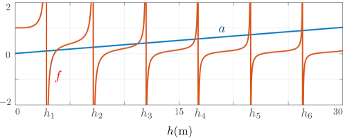
Figure 7: Variations of the impedance parameters $a=Z/(k_{\text{\tiny T}}\rho_{\text{\tiny s}})$ in (50), and $(Z,f)$ in (7), versus $h$. The parameter $f$ diverges at the resonances of the clamped - free plates for $\text{ch}\kappa h\cos\kappa h=-1$.

It is worth noting that the impedance condition implying the resonant contribution is used in [22] in the same configuration considering a spring-mass model. Neglecting the damping used in this reference and adapting the notation, the impedance parameter $f$ is reduced to $f=1/(1-\omega^{2}/\omega_{n}^{2})$ with $\omega_{n}$ a resonance frequency. This relation has to be understood locally in the vicinity of a single resonance, and from $f$ in figure 7, it is visible that (i) it captures the physics of a single resonance locally (ii) it should be corrected by a constant $C_{n}$ depending on the considered resonance $f=C_{n}/(1-\omega^{2}/\omega_{n}^{2})$ to account for the increase in sharpness of the bending resonances when $h$ or $\omega$ increases.

4.2.1 Weak interaction

Far from the resonances, the interaction is weak. Indeed, from (6), with $Z$ being small and $f(\kappa h)$ of the order of unity, the wave impinging the surface sees essentially a flat surface, with $\sigma_{11}\simeq\sigma_{12}\simeq 0$ at $x_{1}=0$. The resulting patterns, not reported, are indeed similar to those obtained for a flat interface in figure 6. Since there is not much to be said on the field in the substrate, we focus on the capability of the complete effective solution to reproduce the actual displacement in the plates. Figure 8 show a small region of the displacement fields near the interface ($h=5$ m resulting in $k_{\text{\tiny T}}h=0.7$ and $\theta_{\text{\tiny L}}=45^{\circ}$). From what we have said (the interaction is weak), the displacements in the substrate are neatly reproduced. More interestingly, the displacements in the plates are also accurately reproduced in an ”averaged” sense which clearly appears for the displacement $u_{1}$ : in the actual problem, $u_{1}$ varies linearly with $x_{2}$ within a single plate, in agreement with (21); this variation at the small scale is superimposed to a variation at large scale, from one plate to the other. The small scale variations do not appear in the homogenized solution since they vanish on average while the large scale variation is captured. The same occurs for $u_{2}$ but in this case, the small scale variations are less visible because they appears at the order 2 (see (17) and (27)).

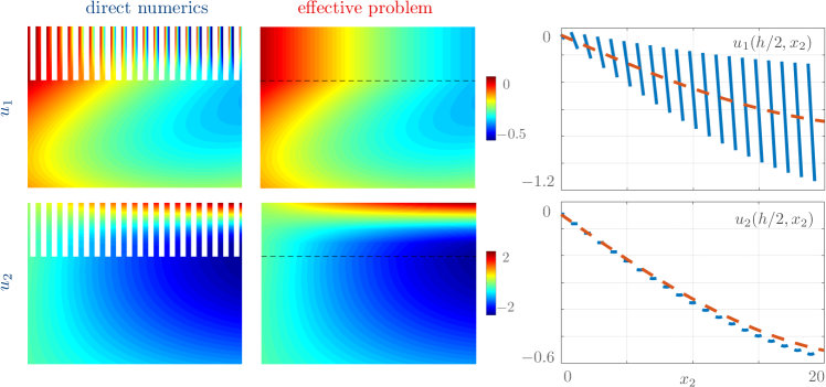
Figure 8: Meaning of the homogenization process – Displacement fields (actual and homogenized) for $x_{1}\in(-10,\;5)$ m and $x_{2}\in(0,\;20)$ m ($h=5$ m, $\theta_{\text{\tiny L}}=45^{\circ}$).

4.2.2 Strong coupling near the resonances

Strong coupling in the vicinity of the bending resonances can be measured by the amplitudes of the displacements in the plates. We report in figure 9 the amplitudes of the horizontal displacements against $h$, at the bottom and at the top of a single plate. In the actual problem these amplitudes are calculated by averaging over $x_{2}\in(-\ell_{\text{\tiny p}}/2,\ell_{\text{\tiny p}}/2)$ the profiles $|u_{2}(0,x_{2})|$ and $|u_{2}(h,x_{2})|$ obtained numerically. In the homogenized problem $|u_{2}(0,x_{2})|$ and $|u_{2}(h,x_{2})|=|V(h)u_{2}(0,x_{2})|$ are given in closed-forms from (51).

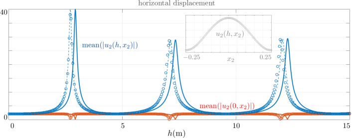
Figure 9: Amplitude of $u_{2}$ at the bottom $x_{1}=0$ and at the top $x_{1}=h$ of a plate against $h$, from direct numerics (symbols) and from the effective solution (51) (plain line); $\theta_{\text{\tiny L}}=45^{\circ}$. Shifts in the resonances $h\to h-h_{0}$, with $h_{0}=0.22$ m are compensated (dashed line). The inset shows the actual variation of $u_{2}(h,x_{2})$ within a single plate with variations as small as about $10^{-4}$ with respect to the mean value.

For $h\in(0,15)$ m, the first three bending resonances are visible by means of high displacements at the top of the plates (up to 40 times the amplitude of the incident wave in the reported case). It is also visible by means of vanishing amplitude at the bottom of the plate, in agreement with (51) for $f\to\infty$. Hence, near the bending resonances, the plates are clamped and they impose a vanishing horizontal displacement at the interface with the substrate, a fact already mentioned in [22].

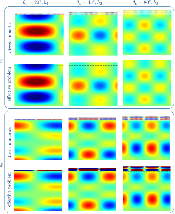
Figure 10: Strong coupling of the array near the three first bending resonances – The values of $h_{n}$, $n=1,2,3$ have been taken from figure 9 at the maximum displacements in the direct numerics and in the homogenized solution. Same representation as in figure 6.

In the substrate, the resulting displacements are significantly impacted. Large values of $f(\kappa h)$ produce $R_{\text{\tiny LL}}\simeq-1$, $R_{\text{\tiny TT}}\simeq 1$ and $R_{\text{\tiny TL}}\simeq R_{\text{\tiny LT}}\simeq 0$ in (50), hence

$$\left\{\begin{array}[]{l}\displaystyle u_{1}(x_{1},x_{2})\simeq 2ik_{\text{\tiny L}}\cos\theta_{\text{\tiny L}}\left(A_{\text{\tiny L}}^{\text{\tiny inc}}\cos\alpha_{\text{\tiny L}}x_{1}+A_{\text{\tiny T}}^{\text{\tiny inc}}\tan\theta_{\text{\tiny L}}\cos\alpha_{\text{\tiny T}}x_{1}\right)e^{i\beta x_{2}},\\[12.0pt] \displaystyle u_{2}(x_{1},x_{2})\simeq 2k_{\text{\tiny T}}\cos\theta_{\text{\tiny T}}\left(-A_{\text{\tiny L}}^{\text{\tiny inc}}\tan\theta_{\text{\tiny L}}\sin\alpha_{\text{\tiny L}}x_{1}+A_{\text{\tiny T}}^{\text{\tiny inc}}\sin\alpha_{\text{\tiny T}}x_{1}\right)e^{i\beta x_{2}},\end{array}\right.$$ (52)

corresponding to a superposition of standing waves. Examples of resulting patterns are shown in figure 10 for the first three bending resonances to be compared with those obtained for a flat interface in figure 6. It is worth noting that in figure 10 we have accounted for the shift in $h_{n}$, $n=1,2,3$ in the homogenized solution from figure 9, where a systematic shift of the effective solution $h\to h-h_{0}$, with $h_{0}=0.22$ m in the present case.

4.3 Occurence of the first longitudinal resonance

To go further in the analysis, we report in figure 11 the reflection coefficients against $h\in(0,25)$ m and $\theta\in(0,90^{\circ})$. We represent the real and imaginary parts of the 4 reflection coefficients. As previously said, our analysis does not hold at and above the first longitudinal resonance, which appears for $h\simeq 25.3$ m (hence $\kappa h=3.4$); expectedly, the effective model indeed breaks down at this high value but it remains surprisingly accurate up to $h\sim 15$ m (hence $k_{\text{\tiny T}}h\sim 2$).

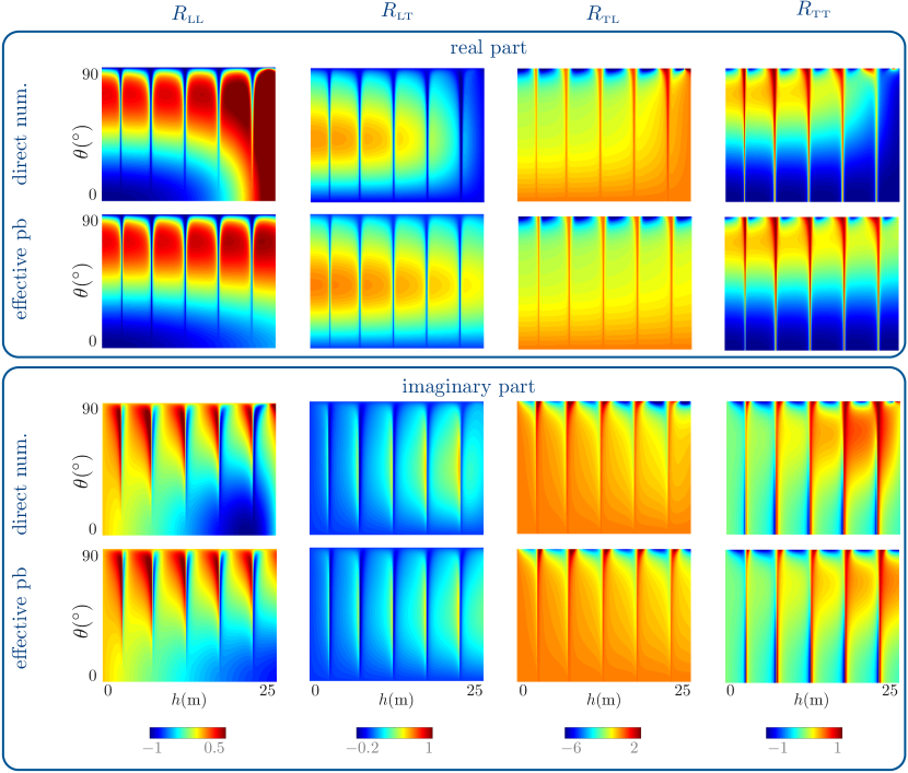
Figure 11: Accuracy of the effective model on the reflection coefficients – Real and imaginary parts of the four reflection coefficients versus $h$ and $\theta$. The solution of the effective problem, (50) (second row) reproduces accurately the direct numerical solution of the actual problem (first row) up to the occurence of the first longitudinal resonance for $h\simeq 25.3$ m.

The occurence of this resonance is visible by means of the amplitude of the vertical displacement $u_{1}(0,x_{2})$, which is reported in figure 12 against $h$. We observe the same trends as for the bending modes. Far from the resonance, the displacement is essentially the same as for a surface on its own; at the longitudinal resonance, it tends to zero resulting in clamped- free conditions for the plates. However, it is also visible that rapid variations of the displacements due to multiple bending resonances superimpose to the smooth variations of the displacement due to the longitudinal resonance.

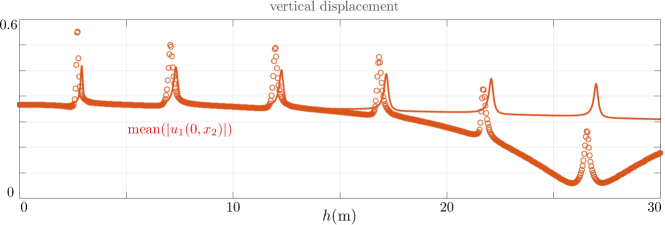
Figure 12: Occurence of the first resonance in reflection – Variation of the amplitude of the vertical displacement $u_{1}(0,x_{2})$ at the bottom of the plates. The bending resonances are superimposed to this resonance which produces a almost clamped condition $u_{1}(0,x_{2})=0$ for $h\simeq 25.3$ m.

5 Conclusion

We have studied the interaction of an array of plates or beams with an elastic half-space using asymptotic analysis and homogenization techniques. The resulting models (3)-(5) for plates and (55)-(57) for beams provide one-dimensional propagation problems which in their simpler form consist in effective boundary conditions at the surface of the ground, (6) for plates and (59) for beams. The exception for plates in the boundary condition $\sigma_{13}$ in (5) is incidental for in-plane incidence but it is interesting since it provides non trivial coupling for arbitrary incidence. For in-plane incidence, the model has been validated by comparison with direct numerical simulations which show an overall good agreement. In particular, the displacement fields obtained in a closed-form accurately reproduce the actual ones; this is of practical importance for applications to site-city interaction where the displacements at the bottom and at the top of buildings are relevant quantities to measure the risk of building damage.

Our models have been obtained owing to a deductive approach which applies to a wide variety of problems. An important point is that the analysis does not assume a preliminary model reduction for the resonator on its own and as such, it can be conducted at any order. Higher order models would involve enriched transmission and boundary conditions able to capture more subtle effects as the shift in the resonance frequencies visible in the figure 9 or the presence of heterogeneity at the roots and at the top of the bodies as it has been done in [36]. Next, we have considered bodies with sufficient symmetry resulting in a diagonal rigidity matrices and which allow for easier calculations. When symmetries are lost, and the simplest case is that of beams with rectangular cross-sections, the calculations are similar; they will produce couplings for incidences as soon as the horizontal component does not coincide with one of the two principal directions. Additional complexities can be accounted for straightforwardly, as orthotropic anisotropy along $x_{1}$ or slow variations in the cross-section. Eventually, the models are restricted to the low frequency regime where only the flexural resonances take place. At the threshold of the first longitudinal resonance, they fail as illustrated in figure 12. Extension of the present work consists in adapting the homogenization procedure in order to capture both flexural and longitudinal resonances at higher frequencies.

Acknowledgements

A. M. and S.G. acknowledge insightful discussions with Philippe Roux at the Institute ISTerre of the University of Grenoble-Alpes. S.G. is also thankful for a visiting position in the group of Richard Craster within the Department of Mathematics at imperial College London in 2018-2019.

Appendix A Remark on the solution in the region of the plates

From the boundary conditions (5), $\frac{\partial^{2}u_{2}}{\partial x_{1}^{2}}(h,x_{2})=\frac{\partial^{3}u_{2}}{\partial x_{1}^{3}}(h,x_{2})=0$ and ${u_{2}}(0^{+},x_{2})={u_{2}}(0^{-},x_{2})$, $\frac{\partial u_{2}}{\partial x_{1}}(0^{+},x_{2})=0$, the general solution for $x_{1}\in(0,h)$ reads as follows

$$\left\{\begin{array}[]{l}\displaystyle u_{2}(x_{1},x_{2})=A(x_{2})\left\{a(\kappa h)\left[\text{ch}\kappa(x_{1}-h)+\cos\kappa(x_{1}-h)\right]+b(\kappa h)\left[\text{sh}\kappa(x_{1}-h)+\sin\kappa(x_{1}-h)\right]\right\},\\[10.0pt] \text{with }\quad a(\kappa h)=(\text{ch}\kappa h+\cos\kappa h),\quad b(\kappa h)=(\text{sh}\kappa h-\sin\kappa h).\end{array}\right.$$ (53)

The displacement $u_{2}$ is continuous at $x_{1}=0$ and we have $2A(x_{2})(1+\text{ch}\kappa h\,\cos\kappa h)=u_{2}(0,x_{2})$, hence

$$\left\{\begin{array}[]{l}{u_{2}}(x_{1},x_{2})=u_{2}(0,x_{2})V(x_{1}),\\[10.0pt] \displaystyle V(x_{1})=\frac{a(\kappa h)\left[\text{ch}\kappa(x_{1}-h)+\cos\kappa(x_{1}-h)\right]+b(\kappa h)\left[\text{sh}\kappa(x_{1}-h)+\sin\kappa(x_{1}-h)\right]}{2\left(1+\text{ch}\kappa h\cos\kappa h\right)}.\end{array}\right.$$ (54)

Obviously, this holds except at the resonance frequencies of the plates for $\text{ch}\kappa_{r}h\,\cos\kappa_{r}h=-1$ which imposes $u_{2}(0,x_{2})=0$ (and eigenmodes in the region of the plates). It follows that the relation on $\sigma_{12}(0^{-},{\bf x}^{\prime})$ in (5) becomes $\sigma_{12}(0^{-},{\bf x}^{\prime})=-(D_{\text{\tiny p}}/\ell)V^{\prime\prime\prime}(0)\;u_{2}(0,x_{2})$, with $V^{\prime\prime\prime}(0)=-\kappa^{4}hf(\kappa h)$, with $f(\kappa h)$ in (6). With $\sigma_{12}(0^{-},{\bf x}^{\prime})=(\kappa^{4}D_{\text{\tiny p}}h/\ell)f(\kappa h)\;u_{2}(0,x_{2})$ and $\kappa^{4}D_{\text{\tiny p}}=\rho_{\text{\tiny p}}\omega^{2}\varphi\ell$, we recover the form announced in (6).

Figure 13: Bending resonances in the region of the plates (clamped/stress free conditions).

Appendix B Main steps of the derivation for an array of circular beams

Let us derive in this Appendix the effective model for circular beams of radius $r_{\text{\tiny p}}$, for which all the derivations are analytical; the circular beams are periodically located in a square array whose unit cell has a section area $S$ (figure 1(b)). In this case, the complete formulation of the problem reads

$$\left\{\begin{array}[]{ll}\displaystyle\text{In the substrate},x_{1}\in(-\infty,0):&\text{div}{\bm{\sigma}}+\rho_{\text{\tiny s}}\omega^{2}{\bf u}={\bf 0},\quad{\bm{\sigma}}=2\mu_{\text{\tiny s}}{\bm{\varepsilon}}+\lambda_{\text{\tiny s}}\text{tr}({\bm{\varepsilon}}){\mathsf{\bm{missing}}I},\\[12.0pt] \displaystyle\text{In the region of the beams},x_{1}\in(0,h):&\displaystyle\frac{\partial^{4}u_{\alpha}}{\partial x_{1}^{4}}-\kappa^{4}u_{\alpha}=0,\quad\alpha=2,3,\quad\kappa=\left(\frac{\rho_{\text{\tiny p}}\omega^{2}\pi r_{\text{\tiny p}}^{2}}{D_{\text{\tiny p}}}\right)^{1/4},\end{array}\right.$$ (55)

where

$$D_{\text{\tiny p}}=E_{\text{\tiny p}}\,\frac{\pi r_{\text{\tiny p}}^{4}}{4},$$ (56)

is the flexural rigidity of the circular beams, complemented by the boundary conditions

$$\left\{\begin{array}[]{l}\displaystyle\sigma_{11}(0^{-},{\bf x}^{\prime})=\rho_{\text{\tiny p}}\omega^{2}\varphi h\;u_{1}(0,x_{2}),\\[10.0pt] \displaystyle\sigma_{1\alpha}(0^{-},{\bf x}^{\prime})=-\frac{D_{\text{\tiny p}}}{S}\,\;\frac{\partial^{3}u_{\alpha}}{\partial x_{1}^{3}}(0^{+},x_{2}),\\[10.0pt] \displaystyle{u_{\alpha}}(0^{+},{\bf x}^{\prime})={u_{\alpha}}(0^{-},{\bf x}^{\prime}),\quad\displaystyle\frac{\partial u_{\alpha}}{\partial x_{1}}(0^{+},{\bf x}^{\prime})=0,\\[10.0pt] \displaystyle\frac{\partial^{2}u_{\alpha}}{\partial x_{1}^{2}}(h,{\bf x}^{\prime})=\frac{\partial^{3}u_{\alpha}}{\partial x_{1}^{3}}(h,{\bf x}^{\prime})=0,\quad\alpha=2,3.\end{array}\right.$$ (57)

where $\varphi=\pi r_{\text{\tiny p}}^{2}/S$. It follows that the problem can be thought in the substrate only, with

$$\text{div}{\bm{\sigma}}+\rho_{\text{\tiny s}}\omega^{2}{\bf u}={\bf 0},\quad{\bm{\sigma}}=2\mu_{\text{\tiny s}}{\bm{\varepsilon}}+\lambda_{\text{\tiny s}}\text{tr}({\bm{\varepsilon}})\,{\mathsf{\bm{missing}}I},\quad x_{1}\in(-\infty,0),$$ (58)

along with the boundary conditions of the Robin’s type

$$\left\{\begin{array}[]{l}\displaystyle\sigma_{11}(0,{\bf x}^{\prime})=\;Zu_{1}(0,{\bf x}^{\prime}),\\[10.0pt] \displaystyle\sigma_{1\alpha}(0,{\bf x}^{\prime})=Z\;f(\kappa h)\;u_{\alpha}(0,{\bf x}^{\prime}),\end{array}\right.$$ (59)

where $Z$ and $f(\kappa h)$ are defined in (7) (we used that $D_{\text{\tiny p}}\kappa^{4}=\rho_{\text{\tiny p}}\omega^{2}\pi r_{\text{\tiny p}}^{2}$).

B.1 Effective wave equation in the region of the beams

B.1.1 Notations

We shall use the same expansions as in (9) but now, the terms ${\bf w}^{n}$ and ${\bm{\pi}}^{n}$ depend on ${\bf z}^{\prime}=(z_{2},z_{3})$ (and not only on $z_{2}$) and we seek to establish the effective behaviour in the region of the array in terms of macroscopic averaged fields

$$\overline{{\bf w}^{n}}(y_{1},{\bf x}^{\prime})=\frac{1}{\varphi\hat{S}}\int_{Y}{\bf w}^{n}(y_{1},{\bf z}^{\prime},{\bf x}^{\prime})\,\text{d}{\bf z}^{\prime},\quad\overline{{\bm{\pi}}^{n}}(y_{1},{\bf x}^{\prime})=\frac{1}{\hat{S}}\int_{Y}{\bm{\pi}}^{n}(y_{1},{\bf z}^{\prime},{\bf x}^{\prime})\,\text{d}{\bf z}^{\prime},$$ (60)

where ${\bf x}^{\prime}=(x_{2},x_{3})$ and $Y$ represents the circular section of the beam $Y=\left\{\sqrt{z_{2}^{2}+z_{3}^{2}}\leq\hat{r}\right\}$, with $\hat{r}=r_{\text{\tiny p}}/\eta^{2}$. It is worth noting that it is sufficient to replace $z_{2}$ by ${\bf z}^{\prime}$ in (10) to (15); in particular, we have

$$\nabla\to\frac{{\bm{e}}_{1}}{\eta}\frac{\partial}{\partial y_{1}}+\frac{1}{\eta^{2}}\nabla_{{\bf z}^{\prime}}+\nabla_{{\bf x}^{\prime}}.$$ (61)

and

$${\bm{\varepsilon}}^{{\bf z}^{\prime}}({\bf w})=\frac{1}{2}\begin{pmatrix}0&\frac{1}{2}\partial_{z_{2}}{w_{1}}&\frac{1}{2}\partial_{z_{3}}{w_{1}}\\[8.0pt] \frac{1}{2}\partial_{z_{2}}{w_{1}}&\partial_{z_{2}}{w_{2}}&\frac{1}{2}\left(\partial_{z_{3}}{w_{2}}+\partial_{z_{2}}{w_{3}}\right)\\[8.0pt] \frac{1}{2}\partial_{z_{3}}{w_{1}}&\frac{1}{2}\left(\partial_{z_{3}}{w_{2}}+\partial_{z_{2}}{w_{3}}\right)&\partial_{z_{3}}{w_{3}}\end{pmatrix}.$$ (62)

B.1.2 Sequence of resolution and main results of the analysis

The analysis is made more involved since the problem is two-dimensional in the rescaled coordinate ${\bf z}^{\prime}$. The procedure is thus more complex. It is as follow:

1. We establish that

   $$\overline{\pi^{0}_{11}}=0,$$ (63)

   and the dependence of ${\bf w}^{0}$ on $(z_{2},z_{3})$, specifically

   $$w^{0}_{1}=W^{0}_{1}({\bf x}^{\prime}),\quad w^{0}_{\alpha}=W^{0}_{\alpha}(y_{1},{\bf x}^{\prime}),$$ (64)

2. We deduce the form of ${\bm{\pi}}^{0}$ and of ${\bf w}^{1}$

   $$\left\{\begin{array}[]{l}\displaystyle\pi_{11}^{0}=-E_{\text{\tiny p}}\frac{\partial^{2}W^{0}_{\alpha}}{\partial y_{1}^{2}}(y_{1},{\bf x}^{\prime})\;z_{\alpha},\quad\displaystyle\pi_{1\alpha}^{0}=\pi_{\alpha\beta}^{0}=0,\\ \displaystyle w^{1}_{1}=W_{1}^{1}({\bf x}^{\prime})-\frac{\partial W^{0}_{\alpha}}{\partial y_{1}}(y_{1},{\bf x}^{\prime})\,z_{\alpha},\quad w^{1}_{\alpha}=W^{1}_{\alpha}(y_{1},{\bf x}^{\prime}).\end{array}\right.$$ (65)

3. eventually the form of $\overline{\pi^{1}_{1i}}$ and the Euler-Bernoulli equation for the bending $W^{0}_{\alpha}$, $\alpha=2,3$. Specifically

   $$\left\{\begin{array}[]{l}\displaystyle\overline{\pi_{11}^{1}}(y_{1},{\bf x}^{\prime})=\rho_{\text{\tiny p}}\omega^{2}\varphi\,W_{1}^{0}({\bf x}^{\prime})\,(\hat{h}-y_{1}),\\[10.0pt] \displaystyle\overline{\pi^{1}_{1\alpha}}(y_{1},{\bf x}^{\prime})=-E_{\text{\tiny p}}\,\frac{\varphi\hat{r}^{2}}{4}\frac{\partial^{3}W_{\alpha}^{0}}{\partial y_{1}^{3}}(y_{1},{\bf x}^{\prime}),\end{array}\right.$$ (66)

   and

   $$E_{\text{\tiny p}}\,\frac{\hat{r}^{2}}{4}\,\frac{\partial^{4}W^{0}_{\alpha}}{\partial y_{1}^{4}}-\rho_{\text{\tiny p}}\omega^{2}\,W^{0}_{\alpha}=0.$$ (67)

B.1.3 First step: $\overline{\pi^{0}_{11}}$ in (63) and ${\bf w}^{0}$ in (64)

This step is not very demanding. From $(\text{E}_{1})^{-1}$ in (13), $\partial_{y_{1}}{\pi^{0}_{11}}+\partial_{z_{\alpha}}{\pi^{1}_{1\alpha}}=0$, which after integration over $Y$ leaves us with $\partial_{y_{1}}\overline{\pi^{0}_{11}}=0$; anticipating $\overline{\pi_{11}^{0}}=0$ at the top of the beams (as we did for the plates), we get $\overline{\pi^{0}_{11}}=0$ everywhere, as announced in (63).

Now, from $(\text{C}^{\prime}_{1\alpha})^{-2}$ in (14), $\partial_{z_{\alpha}}{w^{0}_{1}}=0$ and from $(\text{C}^{\prime}_{11})^{-1}$ $\partial_{y_{1}}w^{0}_{1}=0$. It follows that $w_{1}^{0}$ depends only on ${\bf x}^{\prime}$, in agreement with (64). From $(\text{C}^{\prime}_{\alpha\beta})^{-2}$, $w^{0}_{\alpha}$ is a rigid body motion i.e.

$$w^{0}_{\alpha}=W^{0}_{\alpha}(y_{1},{\bf x}^{\prime})+{\Omega}^{0}(y_{1},{\bf x}^{\prime})({\bm{e}}_{1},{\bf z},{\bm{e}}_{\alpha}),$$ (68)

with $({\bm{e}}_{1},{\bf z},{\bm{e}}_{\alpha})={\bm{e}}_{1}\cdot({\bf z}\times{\bm{e}}_{\alpha})$ being the triple product, and we shall establish that ${\Omega}^{0}=0$. To do so we infer, from $(\text{C}^{\prime}_{1\alpha})^{-1}$, that

$$\partial_{z_{\alpha}}w^{1}_{1}+\partial_{y_{1}}w^{0}_{\alpha}=0\rightarrow\partial_{y_{1}}\left(\partial_{z_{2}}w^{0}_{3}-\partial_{z_{3}}w^{0}_{2}\right)=0.$$ (69)

Inserting (68) in (69) tells us that ${\Omega}^{0}$ does not depend on $y_{1}$ and anticipating the matching condition with the displacement in the substrate which imposes that ${\Omega}^{0}=0$ at $y_{1}=0$, we deduce that ${\Omega}^{0}=0$ everywhere, and (68) reduces to the form of $w^{0}_{\alpha}$ announced in (64).

B.1.4 Second step: ($\pi^{0},{\bf w}^{1}$) in (65)

We start by determining ${\bf w}^{1}$ incompletely (compared to what is announced in (64)). For $w_{1}^{1}$, we come back to $\partial_{z_{\alpha}}w^{1}_{1}+\partial_{y_{1}}w^{0}_{\alpha}=0$ in (69), and $w^{0}_{\alpha}$ in (64) provides us with

$$w_{1}^{1}=W_{1}(y_{1},{\bf x}^{\prime})-\frac{\partial W_{\alpha}^{0}}{\partial y_{1}}(y_{1},{\bf x}^{\prime})\,z_{\alpha},$$ (70)

and it remains for us to show that $W_{1}$ does not depend on $y_{1}$; this will be done after $\pi_{11}^{0}$ has been determined. Next, from $(\text{C}^{\prime}_{\alpha\beta})^{-1}$, $w^{1}_{\alpha}$ is a rigid body motion, hence

$$w^{1}_{\alpha}=W^{1}_{\alpha}(y_{1},{\bf x}^{\prime})+{\Omega}^{1}(y_{1},{\bf x}^{\prime})({\bm{e}}_{1},{\bf z},{\bm{e}}_{\alpha}).$$ (71)

Now, we shall prove that ${\Omega}^{1}=0$; this will be done once $\pi^{0}_{1\alpha}$ have been determined. For the time being, we pursue the calculations by setting the boundary value problem set in $Y$ on the unknowns $(\pi^{0}_{\alpha\beta},w^{2}_{\alpha})$. From $(\text{E}_{\alpha})^{-2}$ and $(\text{C}_{\alpha\beta})^{0}$ in (13), it reads

$$\left\{\begin{array}[]{l}\partial_{z_{\beta}}{\pi^{0}_{\alpha\beta}}=0,\quad\pi^{0}_{\alpha\beta}=2\mu_{\text{\tiny p}}\left({\bm{\varepsilon}}^{{\bf x}^{\prime}}_{\alpha\beta}({\bf w}^{0})+{\bm{\varepsilon}}^{{\bf z}^{\prime}}_{\alpha\beta}({\bf w}^{2})\right)+\lambda_{\text{\tiny p}}\left(\partial_{y_{1}}{w^{1}_{1}}+{\bm{\varepsilon}}^{{\bf x}^{\prime}}_{\gamma\gamma}({\bf w}^{0})+{\bm{\varepsilon}}^{{\bf z}^{\prime}}_{\gamma\gamma}({\bf w}^{2})\right)\delta_{\alpha\beta},\quad\text{in }Y,\\[10.0pt] \pi^{0}_{\alpha\beta}n_{\beta}=0\quad\text{on}\quad\partial Y,\end{array}\right.$$ (72)

with ${\bf w}^{0}$ known from (64) and $w^{1}_{1}$ from (70) at this stage. It is easy to check that the solution of this boundary value problem is

$$\left\{\begin{array}[]{l}\pi^{0}_{\alpha\beta}=0,\\ \displaystyle w^{2}_{\alpha}=-e^{{\bf x}^{\prime}}_{\alpha\beta}({\bf w}^{0})z_{\beta}-\frac{\lambda_{\text{\tiny p}}}{2(\mu_{\text{\tiny p}}+\lambda_{\text{\tiny p}})}z_{\alpha}\frac{\partial W_{1}}{\partial y_{1}}(y_{1},{\bf x}^{\prime})+\frac{\lambda_{\text{\tiny p}}}{2(\mu_{\text{\tiny p}}+\lambda_{\text{\tiny p}})}g_{\alpha}+W^{2}_{\alpha}(y_{1},{\bf x}^{\prime})+{\Omega}^{2}(y_{1},{\bf x}^{\prime})({\bm{e}}_{1},{\bf z},{\bm{e}}_{\alpha}),\end{array}\right.$$ (73)

where

$$g_{2}=\left(\frac{z_{2}^{2}}{2}-\frac{z_{3}^{2}}{2}\right)\frac{\partial^{2}W^{0}_{2}}{\partial y_{1}^{2}}+z_{2}z_{3}\frac{\partial^{2}W^{0}_{3}}{\partial y_{1}^{2}},\quad g_{3}=\left(\frac{z_{3}^{2}}{2}-\frac{z_{2}^{2}}{2}\right)\frac{\partial^{2}W^{0}_{3}}{\partial y_{1}^{2}}+z_{2}z_{3}\frac{\partial^{2}W^{0}_{2}}{\partial y_{1}^{2}}.$$ (74)

The above form of $w_{\alpha}^{2}$ along with $w_{\alpha}^{0}$ in (64) can now be used to find $\pi^{0}_{11}=\left(2\mu_{\text{\tiny p}}+\lambda_{\text{\tiny p}}\right)\partial_{y_{1}}{w^{1}_{1}}+\lambda_{\text{\tiny p}}\left(\partial_{x_{\alpha}}{w^{0}_{\alpha}}+\partial_{z_{\alpha}}{w^{2}_{\alpha}}\right)$, and we get

$$\pi^{0}_{11}=E_{\text{\tiny p}}\left(\frac{\partial W_{1}}{\partial y_{1}}(y_{1},{\bf x}^{\prime})-\frac{\partial^{2}W^{0}_{\alpha}}{\partial y_{1}^{2}}(y_{1},{\bf x}^{\prime})\,z_{\alpha}\right),$$ (75)

where we used that $E_{\text{\tiny p}}=\mu_{\text{\tiny p}}(2\mu_{\text{\tiny p}}+3\lambda_{\text{\tiny p}})/(\mu_{\text{\tiny p}}+\lambda_{\text{\tiny p}})$. It is now sufficient to remember that $\overline{\pi^{0}_{11}}=0$ to get that $\partial_{y_{1}}{W_{1}}=0$, hence the above expression of $\pi^{0}_{11}$ simplifies to the form announced in (65) and $w^{1}_{1}$ in (70) simplifies to to that in (65).

We now use the boundary value problem set in $Y$ on the unknowns $(\pi^{0}_{1\alpha},w^{2}_{1})$. From $(\text{E}_{1})^{-2}$ and $(\text{C}_{1\alpha})^{0}$ in (13), it reads as follows

$$\left\{\begin{array}[]{l}\partial_{z_{\alpha}}{\pi^{0}_{1\alpha}}=0,\quad\pi^{0}_{1\alpha}=\mu_{\text{\tiny p}}\left(\partial_{y_{1}}{w^{1}_{\alpha}}+\partial_{x_{\alpha}}{w^{0}_{1}}+\partial_{z_{\alpha}}{w^{2}_{1}}\right),\quad\text{in }Y,\\ \pi^{0}_{1\alpha}n_{\alpha}=0,\quad\text{on}\quad\partial Y,\end{array}\right.$$ (76)

with $w^{0}_{1}$ known from (64) and $w^{1}_{\alpha}$ from (71) at this stage. The solution is again found to be of the form

$$\left\{\begin{array}[]{l}\displaystyle\pi^{0}_{1\alpha}=\mu_{\text{\tiny p}}\,\frac{\partial{\Omega}^{1}}{\partial y_{1}}(y_{1},{\bf x}^{\prime})({\bm{e}}_{1},{\bf z},{\bm{e}}_{\alpha}),\\ \displaystyle w^{2}_{1}=W^{2}_{1}(y_{1},{\bf x}^{\prime})-z_{\alpha}\left(\frac{\partial W^{1}_{\alpha}}{\partial y_{1}}(y_{1},{\bf x}^{\prime})+\frac{\partial W^{0}_{1}}{\partial x_{\alpha}}({\bf x}^{\prime})\right),\end{array}\right.$$ (77)

and we see that ${\Omega}^{1}=0$ implies $\pi^{0}_{1\alpha}=0$. To show that ${\Omega}^{1}=0$, we use $\partial_{y_{1}}{\pi^{0}_{1\alpha}}+\partial_{z_{\beta}}{\pi^{1}_{\alpha\beta}}=0$ which we infer from $(\text{E}_{\alpha})^{-1}$. Multiplying by ${\bf v}=v_{\alpha}{\bm{e}}_{\alpha}$ with the triple product $v_{\alpha}=({\bm{e}}_{1},{\bf z},{\bm{e}}_{\alpha})$ and integrating over $Y$, we find that

$$\int_{Y}v_{\alpha}\partial_{y_{1}}{\pi^{0}_{1\alpha}}\;\text{d}{\bf z}^{\prime}+\int_{\partial Y}v_{\alpha}\pi^{1}_{\alpha\beta}n_{\beta}\;\text{d}l-\int_{Y}\partial_{z_{\beta}}{v_{\alpha}}\pi^{1}_{\alpha\beta}\;\text{d}{\bf z}^{\prime}=0.$$ (78)

Since ${\bm{\pi}}^{1}$ is symmetric and $\nabla{\bf v}$ is anti-symmetric, we have $\partial_{z_{\beta}}{v_{\alpha}}\pi^{1}_{\alpha\beta}=0$, and $\pi^{1}_{\alpha\beta}n_{\beta}=0$ on $\partial Y$. Hence, (78) reduces to

$$\int_{Y}v_{\alpha}\frac{\partial\pi^{0}_{1\alpha}}{\partial y_{1}}\;\text{d}{\bf z}^{\prime}=0\rightarrow\frac{\partial^{2}{\Omega}^{1}}{\partial y_{1}^{2}}(y_{1},{\bf x}^{\prime})\int_{Y}({\bm{e}}_{1},{\bf z},{\bm{e}}_{\alpha})^{2}\text{d}{\bf z}^{\prime}=0.$$ (79)

Next, with $({\bm{e}}_{1},{\bf z},{\bm{e}}_{\alpha})^{2}={\bf z}^{2}$ whose integral does not vanish, we obtain that $\partial_{y_{1}}{{\Omega}^{1}}$ does not depend on $y_{1}$; anticipating that $\partial_{y_{1}}{{\Omega}^{1}}(\hat{h},{\bf x}^{\prime})=0$ and ${\Omega}^{1}(\hat{h},{\bf x}^{\prime})=0$, we deduce that ${\Omega}^{1}=0$ everywhere. It follows that $\pi^{0}_{1\alpha}=0$, from (77), and that $w^{1}_{\alpha}=W^{1}_{\alpha}(y_{1},{\bf x}^{\prime})$, from (71), in agreement with (65).

B.1.5 Third step: $\overline{\pi_{1i}^{1}}$ in (66) and the Euler-Bernoulli equations in (67)

This starts with $(\text{E})^{0}$ in (13) integrated over $Y$, specifically

$$\frac{\partial\overline{\pi^{1}_{11}}}{\partial y_{1}}+\rho_{\text{\tiny p}}\omega^{2}\varphi\,W_{1}^{0}=0,\quad\displaystyle\frac{\partial\overline{\pi^{1}_{1\alpha}}}{\partial y_{1}}+\rho_{\text{\tiny p}}\omega^{2}\varphi\,W_{\alpha}^{0}=0,$$ (80)

where we have used that $\overline{{\bm{\pi}}^{0}}=0$ from (63) and (65) and ${\bm{\pi}}^{2}{\bf n}_{|{\,\partial Y}}={\bf 0}$. Since $W_{1}^{0}$ depends only on ${\bf x}^{\prime}$, and anticipating that $\overline{\pi^{1}_{11}}(\hat{h},{\bf x}^{\prime})=0$, we obtain by integration the form of $\overline{\pi^{1}_{11}}$ in (66).

To get $\overline{\pi_{1\alpha}^{1}}$, we multiply $(\text{E}_{1})^{-1}$ (which reads $\partial_{y_{1}}{\pi^{0}_{11}}+\partial_{z_{\beta}}{\pi^{1}_{1\beta}}=0$, with $\pi^{0}_{11}$ in (65)) by $z_{\alpha}$ and integrate over $Y$ to find that

$$E_{\text{\tiny p}}\frac{\partial^{3}W^{0}_{\beta}}{\partial y_{1}^{3}}(y_{1},{\bf x}^{\prime})\int_{Y}z_{\alpha}z_{\beta}\;\text{d}s+\int_{Y}\pi^{1}_{1\beta}\,\delta_{\alpha\beta}\;\text{d}s=0,$$ (81)

where we have used that ${\pi^{1}_{1\beta}\,n_{\beta}}_{|{\,\partial Y}}=0$. For the circular cross-section of the beams, $\int_{Y}z_{2}z_{3}\text{d}{\bf z}^{\prime}=0$ and $\int_{Y}z_{2}^{2}\text{d}{\bf z}^{\prime}=\int_{Y}z_{3}^{2}\text{d}{\bf z}^{\prime}=\pi\hat{r}^{4}/4$. It follows that

$$\hat{S}\overline{\pi^{1}_{1\alpha}}(y_{1},{\bf x}^{\prime})=-E_{\text{\tiny p}}\frac{\pi\hat{r}^{4}}{4}\,\frac{\partial^{3}W^{0}_{\alpha}}{\partial y_{1}^{3}}(y_{1},{\bf x}^{\prime}),$$ (82)

in agreement with (66) (with $\varphi\hat{S}=\pi\hat{r}^{2}$). Coming back to (80) with the above form of $\overline{\pi^{1}_{1\alpha}}$, we deduce that

$$E_{\text{\tiny p}}\frac{\pi\hat{r}^{4}}{4}\,\frac{\partial^{4}W^{0}_{\alpha}}{\partial y_{1}^{4}}-\rho_{\text{\tiny p}}\omega^{2}\varphi\hat{S}W^{0}_{\alpha}=0,$$ (83)

in agreement with (67).

B.2 Effective boundary conditions at the top of the array of beams

As we have done in (30), we consider the following expansions for the displacement and stress

$${\bf u}=\sum_{n\geq 0}\eta^{n}{\bf v}^{n}({\bf z},{\bf x}^{\prime}),\quad{\bm{\sigma}}=\sum_{n\geq 0}\eta^{n}{\bm{\tau}}^{n}({\bf z},{\bf x}^{\prime}).$$ (84)

We use $(\text{e})$ in (33) (with ${\bf z}^{\prime}\to{\bf z}$) which provide us with $\text{div}_{\bf z}{\bm{\tau}}^{0}=\text{div}_{\bf z}{\bm{\tau}}^{1}={\bf 0}$, and this makes the calculations identical to those conducted in §3.2 for the plates when integrating over $Z=\left\{z_{1}\in(-\infty,0),{\bf z}^{\prime}\in Y\right\}$. We thus obtain

$$\overline{\pi^{0}_{1i}}(\hat{h},{\bf z}^{\prime},{\bf x}^{\prime})=\overline{\pi^{1}_{1i}}(\hat{h},{\bf z}^{\prime},{\bf x}^{\prime})=0,\quad i=1,2,3,$$ (85)

(see (35)). The conditions on $\overline{\pi^{0}_{1i}}$ are consistent with (63) and (65). The condition on $\overline{\pi_{11}^{1}}$ is that anticipated to find (66). Eventually, the condition on $\overline{\pi_{1\alpha}^{1}}$ combined with (66) provides the conditions of zero shear force

$$\frac{\partial^{3}W_{\alpha}^{0}}{\partial y_{1}^{3}}(\hat{h},{\bf x}^{\prime})=0.$$ (86)

To derive the condition of zero bending moment, we proceed the same as we have done in (78); with ${\bf v}=v_{\alpha}{\bm{e}}_{\alpha}$ and $v_{\alpha}=({\bm{e}}_{1},{\bf z},{\bm{e}}_{\alpha})$, we consider the vanishing integral $\int_{Z}v_{\alpha}\partial_{z_{i}}\tau_{i\alpha}^{0}\;\text{d}v=0$, hence

$$\int_{\partial Z}v_{\alpha}\tau^{0}_{i\alpha}n_{i}=0,$$ (87)

where we have used that $\partial_{z_{i}}v_{\alpha}\tau^{0}_{i\alpha}=0$ by construction. Because ${\bm{\tau}}^{0}\cdot{\bf n}$ vanishes on $\partial Z$ except at the bottom face $z_{1}=-z_{m}$ and passing to the limit $z_{m}\to+\infty$, this integral reduces to

$$\int_{Y}v_{\alpha}\,\pi^{0}_{1\alpha}(\hat{h},{\bf z}^{\prime},{\bf x}^{\prime})\;\text{d}s=0.$$ (88)

Making use of (77) leads to the anticipated boundary condition

$$\frac{\partial{\Omega}^{1}}{\partial y_{1}}(\hat{h},{\bf x}^{\prime})=0,$$ (89)

that we have used to get $\pi_{1\alpha}^{0}=0$. It remains to derive the condition of zero bending moment. By considering ${\bf a}=z_{\alpha}\,{\bm{e}}_{1}-z_{1}{\bm{e}}_{\alpha}$ and integrating over $Z$ the scalar ${\bf a}\cdot\text{div}_{\bf z}{\bm{\tau}}^{0}$ (since $\text{div}_{\bf z}{\bm{\tau}}^{0}={\bf 0}$), we found that

$$0=\int_{\partial Z}a_{i}\;\tau^{0}_{ij}n_{j}\;\text{d}s=-\int_{Y}\,z_{\alpha}\,{\tau^{0}_{11}}_{|{z_{1}=-z_{m}}}\;\text{d}s-z_{m}\int_{Y}\,{\tau^{0}_{1\alpha}}_{|{z_{1}=-z_{m}}}\;\text{d}s.$$ (90)

Since we have in addition $0=\int_{\partial Z}\,\tau^{0}_{ij}n_{j}\;\text{d}s=\int_{Y}\,{\tau^{0}_{1\alpha}}_{|{z_{1}=-z_{m}}}\;\text{d}s$, we can pass to the limit $z_{m}\to\infty$, and get $0=\int_{Y}z_{\alpha}\tau^{0}_{11}\to\overline{z_{\alpha}\pi^{0}_{11}}(\hat{h},{\bf x}^{\prime})$. Now accounting for $\pi^{0}_{11}$ in (75), we obtain the expected boundary condition

$$\frac{\partial^{2}W_{\alpha}^{0}}{\partial y_{1}^{2}}(\hat{h},{\bf x}^{\prime})=0.$$ (91)

B.3 Effective transmission conditions between the substrate and the array

In the vicinity of the interface between the substrate and the array, we consider the same expansions as in (84), and at the dominant order, we still have $\text{div}_{\bf z}{\bm{\tau}}^{0}=\text{div}_{\bf z}{\bm{\tau}}^{1}={\bf 0}$. The calculations are identical to that conducted in §3.3 when integrating over $Z=\{z_{1}\in(0,+\infty),{\bf z}^{\prime}\in Y\}\cup\{z_{1}\in(-\infty,0),{\bf z}^{\prime}\in(-\hat{\ell}/2,\hat{\ell}/2)^{2}\}$, and we find

$$\sigma_{1i}^{0}(0^{-},{\bf x}^{\prime})=0,\quad i=1,2,3,$$ (92)

which are consistent with (63) and (65). Next, using $\overline{\pi^{1}_{1i}}$ in (66), we find

$$\sigma^{1}_{11}(0^{-},{\bf x}^{\prime})=\rho_{\text{\tiny p}}\omega^{2}\,\varphi\,\hat{h}W^{0}_{1}({\bf x}^{\prime}),\quad\sigma^{1}_{1\alpha}(0^{-},{\bf x}^{\prime})=-E_{\text{\tiny p}}\frac{\pi\hat{r}^{4}}{4S}\frac{\partial^{3}W^{0}_{\alpha}}{\partial y_{1}^{3}}(0,{\bf x}^{\prime}).$$ (93)

We have yet to establish the continuity of the displacement. From the counterpart of $(\text{c}^{\prime})$ in (42) (with ${\bf z}^{\prime}\to{{\bf z}}$), it is easily seen that we have at the dominant orders

$${\bm{\varepsilon}}^{\bf z}({\bf v}^{0})={\bm{\varepsilon}}^{\bf z}({\bf v}^{1})={\bf 0}.$$ (94)

Therefore ${\bf v}^{0}$ and ${\bf v}^{1}$ are piecewise rigid body motions, namely ${\bf v}^{0}={\bm{\Omega}}^{0}({\bf x}^{\prime})\times{\bf z}+{\bf V}^{0}({\bf x}^{\prime})$, the same for ${\bf v}^{1}$. Invoking the periodicity of ${\bf v}^{i}$, $i=1,2$ with respect to $z_{2}$ and $z_{3}$ for $z_{1}<0$ and the continuity of ${\bf v}^{i}$ at $z_{1}=0$, these rigid body motions reduce to a single translation over $Z$. Eventually, using the matching conditions on the displacements, we then obtain

$$u^{0}_{1}(0^{-},{\bf x}^{\prime})=W^{0}_{1}({\bf x}^{\prime}),\quad u^{0}_{\alpha}(0^{-},{\bf x}^{\prime})=W^{0}_{\alpha}(0^{+},{\bf x}^{\prime}),\quad\frac{\partial W^{0}_{\alpha}}{\partial z_{1}}(0^{+},{\bf x}^{\prime})=0.$$ (95)

B.4 The final problem

The effective problem (55) is obtained for $({\bf u}={\bf u}^{0},{\bm{\sigma}}={\bm{\sigma}}^{0}+\eta{\bm{\sigma}}^{1})$ in the substrate for $x_{1}<0$, $({\bf u}={\bf W}^{0},{\bm{\sigma}}={\bm{\pi}}^{0}+\eta{\bm{\pi}}^{1})$ in the region of the array for $x_{1}>0$. Remembering that $y_{1}=x_{1}/\eta$ and $\hat{h}=h/\eta$, $\hat{r}=r_{\text{\tiny p}}/\eta^{2}$, it is easy to see that (i) the Euler-Bernoulli equation in (55) is obtained from (67), (ii) the effective boundary conditions announced in (57) from (86), (91)-(93) and (95).

References

References

- [1] H. Lamb, I. on the propagation of tremors over the surface of an elastic solid, Philosophical Transactions of the Royal Society of London. Series A, Containing papers of a mathematical or physical character 203 (359-371) (1904) 1–42.
- [2] C. Pekeris, The seismic surface pulse, Proceedings of the national academy of sciences of the United States of America 41 (7) (1955) 469.
- [3] P. C. Jennings, J. Bielak, Dynamics of building-soil interaction, Bulletin of the seismological society of America 63 (1) (1973) 9–48.
- [4] E. Kausel, R. V. Whitman, J. P. Morray, F. Elsabee, The spring method for embedded foundations, Nuclear Engineering and design 48 (2-3) (1978) 377–392.
- [5] G. Gazetas, Formulas and charts for impedances of surface and embedded foundations, Journal of geotechnical engineering 117 (9) (1991) 1363–1381.
- [6] E. Kausel, Early history of soil–structure interaction, Soil Dynamics and Earthquake Engineering 30 (9) (2010) 822–832.
- [7] J. E. Luco, L. Contesse, Dynamic structure-soil-structure interaction, Bulletin of the Seismological Society of America 63 (4) (1973) 1289–1303.
- [8] H. Wong, M. Trifunac, Two-dimensional, antiplane, building-soil-building interaction for two or more buildings and for incident planet sh waves, Bulletin of the Seismological Society of America 65 (6) (1975) 1863–1885.
- [9] A. Wirgin, P.-Y. Bard, Effects of buildings on the duration and amplitude of ground motion in mexico city, Bulletin of the Seismological Society of America 86 (3) (1996) 914–920.
- [10] P. Guéguen, P. Bard, J. Semblat, Engineering seismology: seismic hazard and risk analysis: seismic hazard analysis from soil-structure interaction to site-city interaction, in: Proc. 12th World Conference on Earthquake Engineering, 2000.
- [11] D. Clouteau, D. Aubry, Modifications of the ground motion in dense urban areas, Journal of Computational Acoustics 9 (04) (2001) 1659–1675.
- [12] C. Tsogka, A. Wirgin, Simulation of seismic response in an idealized city, Soil Dynamics and Earthquake Engineering 23 (5) (2003) 391–402.
- [13] P. Gueguen, P.-Y. Bard, Soil-structure and soil-structure-soil interaction: experimental evidence at the volvi test site, Journal of Earthquake Engineering 9 (05) (2005) 657–693.
- [14] M. Kham, J.-F. Semblat, P.-Y. Bard, P. Dangla, Seismic site–city interaction: main governing phenomena through simplified numerical models, Bulletin of the Seismological Society of America 96 (5) (2006) 1934–1951.
- [15] J.-P. Groby, A. Wirgin, Seismic motion in urban sites consisting of blocks in welded contact with a soft layer overlying a hard half-space, Geophysical Journal International 172 (2) (2008) 725–758.
- [16] K. Uenishi, The town effect: dynamic interaction between a group of structures and waves in the ground, Rock mechanics and rock engineering 43 (6) (2010) 811–819.
- [17] M. Todorovska, M. Trifunac, The system damping, the system frequency and the system response peak amplitudes during in-plane building-soil interaction, Earthquake engineering & structural dynamics 21 (2) (1992) 127–144.
- [18] P. Gueǵuen, P.-Y. Bard, F. J. Chavez-Garcia, Site-city seismic interaction in mexico city–like environments: an analytical study, Bulletin of the Seismological Society of America 92 (2) (2002) 794–811.
- [19] C. Boutin, P. Roussillon, Assessment of the urbanization effect on seismic response, Bulletin of the Seismological Society of America 94 (1) (2004) 251–268.
- [20] M. Ghergu, I. R. Ionescu, Structure–soil–structure coupling in seismic excitation and city effect??, International Journal of Engineering Science 47 (3) (2009) 342–354.
- [21] C. Boutin, P. Roussillon, Wave propagation in presence of oscillators on the free surface, International journal of engineering science 44 (3-4) (2006) 180–204.
- [22] L. Schwan, C. Boutin, Unconventional wave reflection due to resonant surface, Wave Motion 50 (4) (2013) 852–868.
- [23] C. Boutin, L. Schwan, M. S. Dietz, Elastodynamic metasurface: Depolarization of mechanical waves and time effects, Journal of Applied Physics 117 (6) (2015) 064902.
- [24] L. Schwan, C. Boutin, L. Padrón, M. Dietz, P.-Y. Bard, C. Taylor, Site-city interaction: theoretical, numerical and experimental crossed-analysis, Geophysical Journal International 205 (2) (2016) 1006–1031.
- [25] E. Garova, A. Maradudin, A. Mayer, Interaction of rayleigh waves with randomly distributed oscillators on the surface, Physical Review B 59 (20) (1999) 13291.
- [26] H. Wegert, E. A. Mayer, L. M. Reindl, W. Ruile, A. P. Mayer, Interaction of saws with resonating structures on the surface, in: 2010 IEEE International Ultrasonics Symposium, IEEE, 2010, pp. 185–188.
- [27] A. Maznev, V. Gusev, Waveguiding by a locally resonant metasurface, physical Review B 92 (11) (2015) 115422.
- [28] A. Maznev, Bifurcation of avoided crossing at an exceptional point in the dispersion of sound and light in locally resonant media, Journal of Applied Physics 123 (9) (2018) 091715.
- [29] S. Kuznetsov, Seismic waves and seismic barriers, Acoustical Physics 57 (3) (2011) 420–426.
- [30] S.-H. Kim, M. P. Das, Seismic waveguide of metamaterials, Modern Physics Letters B 26 (17) (2012) 1250105.
- [31] S.-H. Kim, M. P. Das, Artificial seismic shadow zone by acoustic metamaterials, Modern Physics Letters B 27 (20) (2013) 1350140.
- [32] S. Brûlé, E. Javelaud, S. Enoch, S. Guenneau, Experiments on seismic metamaterials: molding surface waves, Physical review letters 112 (13) (2014) 133901.
- [33] S. Krödel, N. Thomé, C. Daraio, Wide band-gap seismic metastructures, Extreme Mechanics Letters 4 (2015) 111–117.
- [34] A. Colombi, P. Roux, S. Guenneau, P. Gueguen, R. V. Craster, Forests as a natural seismic metamaterial: Rayleigh wave bandgaps induced by local resonances, Scientific reports 6 (2016) 19238.
- [35] D. Colquitt, A. Colombi, R. Craster, P. Roux, S. Guenneau, Seismic metasurfaces: Sub-wavelength resonators and rayleigh wave interaction, Journal of the Mechanics and Physics of Solids 99 (2017) 379–393.
- [36] A. Maurel, J.-J. Marigo, K. Pham, S. Guenneau, Conversion of love waves in a forest of trees, Physical Review B 98 (13) (2018) 134311.
- [37] A. Palermo, A. Marzani, Control of love waves by resonant metasurfaces, Scientific reports 8 (1) (2018) 7234.
- [38] A. Palermo, F. Zeighami, A. Marzani, Seismic metasurfaces for love waves control, in: EGU General Assembly Conference Abstracts, Vol. 20, 2018, p. 18607.
- [39] L. Kelders, J. F. Allard, W. Lauriks, Ultrasonic surface waves above rectangular-groove gratings, The Journal of the Acoustical Society of America 103 (5) (1998) 2730–2733.
- [40] J. Zhu, Y. Chen, X. Zhu, F. J. Garcia-Vidal, X. Yin, W. Zhang, X. Zhang, Acoustic rainbow trapping, Scientific reports 3 (2013) 1728.
- [41] J. Pendry, L. Martin-Moreno, F. Garcia-Vidal, Mimicking surface plasmons with structured surfaces, science 305 (5685) (2004) 847–848.
- [42] F. Garcia-Vidal, L. Martin-Moreno, J. Pendry, Surfaces with holes in them: new plasmonic metamaterials, Journal of optics A: Pure and applied optics 7 (2) (2005) S97.
- [43] P. G. Ciarlet, P. Destuynder, A justification of the two-dimensional linear plate model, J Mec 18 (2) (1979) 315–344.
- [44] D. Caillerie, Plaques élastiques minces à structure périodique de période et d’epaisseurs comparables Sc. Paris Sér. II 294 (1982) 159–162.
- [45] L. Trabucho, J. Viano, Derivation of generalized models for linear elastic beams by asymptotic expansion methods, Applications of Multiple Scaling in Mechanics (1987) 302–315.
- [46] G. Geymonat, F. Krasucki, J.-J. Marigo, Sur la commutativité des passages à la limite en théorie asymptotique des poutres composites, Comptes rendus de l’Académie des sciences. Série 2, Mécanique, Physique, Chimie, Sciences de l’univers, Sciences de la Terre 305 (4) (1987) 225–228.
- [47] B. Miara, L. Trabucho, Approximation spectrale pour une poutre en élasticité linéarisée, Comptes rendus de l’Académie des sciences. Série 1, Mathématique 311 (10) (1990) 659–662.
- [48] G. Corre, A. Lebée, K. Sab, M. K. Ferradi, X. Cespedes, Higher-order beam model with eigenstrains: theory and illustrations, ZAMM-Journal of Applied Mathematics and Mechanics/Zeitschrift für Angewandte Mathematik und Mechanik 98 (7) (2018) 1040–1065.
- [49] R. Abdelmoula, J.-J. Marigo, The effective behavior of a fiber bridged crack, Journal of the Mechanics and Physics of Solids 48 (11) (2000) 2419–2444.
- [50] M. David, J.-J. Marigo, C. Pideri, Homogenized interface model describing inhomogeneities located on a surface, Journal of Elasticity 109 (2) (2012) 153–187.
- [51] J.-J. Marigo, A. Maurel, Homogenization models for thin rigid structured surfaces and films, The Journal of the Acoustical Society of America 140 (1) (2016) 260–273.
- [52] A. Maurel, K. Pham, J.-J. Marigo, Scattering of gravity waves by a periodically structured ridge of finite extent, Journal of Fluid Mechanics 871 (2019) 350–376.
- [53] A. Maurel, J.-J. Marigo, J.-F. Mercier, K. Pham, Modelling resonant arrays of the helmholtz type in the time domain, Proceedings of the Royal Society A: Mathematical, Physical and Engineering Sciences 474 (2210) (2018) 20170894.
- [54] A. Maurel, K. Pham, Multimodal method for the scattering by an array of plates connected to an elastic half-space, The Journal of the Acoustical Society of America, to appear.
- [55] J. Achenbach, Wave propagation in elastic solids, Vol. 16, Elsevier, 2012.