Frequency- and Time-Limited Balanced Truncation for Large-Scale Second-Order Systems

Abstract

Considering the use of dynamical systems in practical applications, often only limited regions in the time or frequency domain are of interest. Therefor, it usually pays off to compute local approximations of the used dynamical systems in the frequency and time domain. In this paper, we consider a structure-preserving extension of the frequency- and time-limited balanced truncation methods to second-order dynamical systems. We give a full overview about the first-order limited balanced truncation methods and extend those methods to second-order systems by using the different second-order balanced truncation formulas from the literature. Also, we present numerical methods for solving the arising large-scale sparse matrix equations and give numerical modifications to deal with the problematic case of second-order systems. The results are then illustrated on three numerical examples.

Keywords: model order reduction, second-order differential equations, linear systems, balanced truncation, frequency-limited balanced truncation, time-limited balanced truncation, local model reduction, structure-preserving approximation

1 Introduction

The modeling of, e.g., mechanical and electrical systems often leads to linear dynamical systems containing second-order time derivatives. In this paper, we consider linear second-order input-output systems of the form

$$\begin{aligned} M\ddot{x}+E\dot{x}(t)+Kx(t)&=B_{u}u(t),\\ y(t)&=C_{p}x(t)+C_{v}\dot{x}(t),\end{aligned}$$ (1)

with $M,E,K\in\mathbb{R}^{n\times n}$, $B_{u}\in\mathbb{R}^{n\times m}$ and $C_{p},C_{v}\in\mathbb{R}^{p\times n}$, and $u(t)\in\mathbb{R}^{m}$, the inputs, $x(t)\in\mathbb{R}^{n}$, the states, and $y(t)\in\mathbb{R}^{p}$, the outputs of the system. In the frequency domain, the input-to-output relation is directly given as $y(s)=H(s)u(s)$, whereby the so-called transfer function is given by

$$H(s) =(sC_{v}+C_{p})(s^{2}M+sE+K)^{-1}B_{u},$$ (2)

with $s\in\mathbb{C}$. In applications, the number of differential equations, $n$, describing the system, can become very large. This complicates using the model for simulations and controller design due to the expensive costs in terms of computational resources as time and memory. Therefor, model reduction is needed to construct a surrogate system with a much smaller number of equations $r\ll n$, which approximates the input-to-output behavior of (1). To use the surrogate model as the original one, e.g., applying the same tools, the surrogate needs to have the same structure as the original system, i.e., the reduced-order model should also have the form

$$\begin{aligned} \widehat{M}\ddot{\hat{x}}(t)+\widehat{E}\dot{\hat{x}}(t)+\widehat{K}\hat{x}(t)&=\widehat{B}_{u}u(t),\\ \hat{y}(t)&=\widehat{C}_{p}\hat{x}(t)+\widehat{C}_{v}\dot{\hat{x}}(t),\end{aligned}$$

with the new system matrices $\widehat{M},\widehat{E},\widehat{K}\in\mathbb{R}^{r\times r}$, $\widehat{B}_{u}\in\mathbb{R}^{r\times m}$ and $\widehat{C}_{p},\widehat{C}_{v}\in\mathbb{R}^{p\times r}$.

Due to its relevance in a lot of applications, the problem of structure-preserving model reduction for second-order systems has already been investigated in the literature to quiet an extend. There are structure-preserving extensions of classical model reduction methods like modal truncation and dominant pole algorithms [38, 7, 40], moment matching [2, 41, 15, 42], balanced truncation [33, 16, 37], or for example of the $\mathcal{H}_{2}$-optimal iterative rational Krylov algorithm [47]. Especially, we want to mention the work of Paul Van Dooren, and co-authors, on the second-order balanced truncation approach. In [15], he introduced a new balancing idea that is stronger related to the origins of balanced truncation than the other extensions. Most of the extended methods aim for a globally good approximation behavior, but very often, only the local system’s behavior in the frequency or time domain is of actual interest for the application. In case of first-order systems, the frequency- and time-limited balanced truncation methods, first mentioned in [20], aiming for such local approximations. Those methods have been extended in the first-order case to large-scale sparse systems [6, 28] and to system with differential-algebraic equations [26, 22].

A first attempt to generalize the limited balanced truncation methods to second-order systems has been done in [23] for the frequency-limited balanced truncation by making use of some formulas from [37] and for the time-limited balanced truncation in [24] in the same way. In this paper, we are extending the frequency- and time-limited balanced truncation methods by using all the different second-order balanced truncation approaches from the literature [33, 37, 16] and correct some mistakes that were made in [23, 24] considering the issue of stability preservation. Also, we are extending the numerical approaches to the large-scale second-order system case and present strategies to deal with numerical difficulties aligning with second-order systems in general.

The paper has the following structure. Section 2 contains a review of the theory for the classical and limited balanced truncation methods in the generalized first-order system case; see Section 2.1; as well as a review of the different second-order balanced approaches and the extensions of the limited balanced truncation methods to second-order systems in Section 2.2. Afterwards, in Section 3, the numerical methods for solving the large-scale sparse matrix equations with function right hand-side are covered. Also, the $\alpha$-shift strategy and two-step methods are explained in this section, which ends with the modified Gramian approach and remarks on the stability preservation of the methods. Three numerical examples are then given in Section 4 to demonstrate the applicability of the methods on large-scale sparse second-order systems. Section 5 concludes the paper.

2 The frequency- and time-limited balanced truncation methods

2.1 First-order system case

In this section, we will remind of the classical balanced truncation technique and give an overview on the frequency- and time-limited versions of this method for the case of first-order systems.

2.1.1 Classical balanced truncation

We consider here generalized first-order state-space systems of the form

$$\begin{aligned} \mathcal{E}\dot{q}(t)&=\mathcal{A}q(t)+\mathcal{B}u(t),\\ y(t)&=\mathcal{C}q(t),\end{aligned}$$ (3)

with $\mathcal{E},\mathcal{A}\in\mathbb{R}^{N\times N}$, $\mathcal{B}\in\mathbb{R}^{N\times m}$, $\mathcal{C}\in\mathbb{R}^{p\times N}$, and the corresponding transfer function

$$H(s) =\mathcal{C}(s\mathcal{E}-\mathcal{A})^{-1}\mathcal{B},$$ (4)

with $s\in\mathbb{C}$. For simplicity, we are assuming that $\mathcal{E}$ is invertible and the system is c-stable, i.e., all eigenvalues of $\lambda\mathcal{E}-\mathcal{A}$ lie in the open left complex half-plane. The extension of the balanced truncation method to the descriptor system case ($\mathcal{E}$ non-invertible) can be found in [45, 11]. The system Gramians of (3) are defined as

$$\begin{aligned} P_{\infty}&=\frac{1}{2\pi}\int\limits_{-\infty}^{+\infty}{(j\omega\mathcal{E}-\mathcal{A})^{-1}\mathcal{B}\mathcal{B}^{\mkern-1.5mu\mathsf{T}}(-j\omega\mathcal{E}-\mathcal{A})^{-\mkern-1.5mu\mathsf{T}}\mathrm{d}\omega}=\int\limits_{0}^{+\infty}{e^{\mathcal{E}^{-1}\mathcal{A}t}\mathcal{E}^{-1}\mathcal{B}\mathcal{B}^{\mkern-1.5mu\mathsf{T}}\mathcal{E}^{-\mkern-1.5mu\mathsf{T}}e^{\mathcal{A}^{\mkern-1.5mu\mathsf{T}}\mathcal{E}^{-\mkern-1.5mu\mathsf{T}}t}\mathrm{d}t},\\ Q_{\infty}&=\frac{1}{2\pi}\int\limits_{-\infty}^{+\infty}{(-j\omega\mathcal{E}-\mathcal{A})^{-\mkern-1.5mu\mathsf{T}}\mathcal{C}^{\mkern-1.5mu\mathsf{T}}\mathcal{C}(j\omega\mathcal{E}-\mathcal{A})^{-1}\mathrm{d}\omega}=\int\limits_{0}^{+\infty}{\mathcal{E}^{-\mkern-1.5mu\mathsf{T}}e^{\mathcal{A}^{\mkern-1.5mu\mathsf{T}}\mathcal{E}^{-\mkern-1.5mu\mathsf{T}}t}\mathcal{C}^{\mkern-1.5mu\mathsf{T}}\mathcal{C}e^{\mathcal{E}^{-1}\mathcal{A}t}\mathcal{E}^{-1}\mathrm{d}t},\end{aligned}$$ (5)

with $P_{\infty}$ the infinite controllability Gramian and $\mathcal{E}^{\mkern-1.5mu\mathsf{T}}Q_{\infty}\mathcal{E}$ the infinite observability Gramian. Note that in the infinite case, the frequency and time representations of the Gramians are equal. It can be shown that those Gramians (5) are the unique, symmetric positive semi-definite solutions of the following Lyapunov equations

$$\begin{aligned} \mathcal{A}P_{\infty}\mathcal{E}^{\mkern-1.5mu\mathsf{T}}+\mathcal{E}P_{\infty}\mathcal{A}^{\mkern-1.5mu\mathsf{T}}+\mathcal{B}\mathcal{B}^{\mkern-1.5mu\mathsf{T}}&=0,\\ \mathcal{A}^{\mkern-1.5mu\mathsf{T}}Q_{\infty}\mathcal{E}+\mathcal{E}^{\mkern-1.5mu\mathsf{T}}Q_{\infty}\mathcal{A}+\mathcal{C}^{\mkern-1.5mu\mathsf{T}}\mathcal{C}&=0.\end{aligned}$$ (6)

The Hankel singular values are then defined as the positive square-roots of the eigenvalues of $P_{\infty}\mathcal{E}^{\mkern-1.5mu\mathsf{T}}Q_{\infty}\mathcal{E}$, which are a measure of how much influence the corresponding states have on the input-output behavior of the system. The main idea of balanced truncation is to balance the system such that

$$P_{\infty} =Q_{\infty}=\begin{bmatrix}\sigma_{1}&&&\\ &\sigma_{2}&&\\ &&\ddots&\\ &&&\sigma_{N}\end{bmatrix},$$

with the Hankel singular values $\sigma_{1}\geq\sigma_{2}\geq\ldots\geq\sigma_{N}>0$ and then to truncate states corresponding to small Hankel singular values [34]. The complete balanced truncation square-root method is summarized in Algorithm 1.

1

Input: System matrices $\mathcal{A}$, $\mathcal{B}$, $\mathcal{C}$, $\mathcal{E}$ from (3).

Output: Matrices of the reduced-order system $\widehat{\mathcal{A}}$, $\widehat{\mathcal{B}}$, $\widehat{\mathcal{C}}$, $\widehat{\mathcal{E}}$.

2

3Compute Cholesky factorizations of the Gramians by solving the Lyapunov equations (6) such that $P_{\infty}=R_{\infty}R_{\infty}^{\mkern-1.5mu\mathsf{T}}$, $Q_{\infty}=L_{\infty}L_{\infty}^{\mkern-1.5mu\mathsf{T}}$.

4 Compute the singular value decomposition

$$L_{\infty}^{\mkern-1.5mu\mathsf{T}}\mathcal{E}R_{\infty} =\begin{bmatrix}U_{1}&U_{2}\end{bmatrix}\begin{bmatrix}\Sigma_{1}&\\ &\Sigma_{1}\end{bmatrix}\begin{bmatrix}V_{1}^{\mkern-1.5mu\mathsf{T}}\\ V_{2}^{\mkern-1.5mu\mathsf{T}}\end{bmatrix},$$

with $\Sigma_{1}=\mathrm{diag}(\sigma_{1},\ldots,\sigma_{r})$ containing the $r$ largest Hankel singular values.

5 Construct the projection matrices

$$\begin{aligned} T&=R_{\infty}V_{1}\Sigma_{1}^{-\frac{1}{2}}&&\text{and}&W&=L_{\infty}U_{1}\Sigma_{1}^{-\frac{1}{2}}.\end{aligned}$$

6 Compute the reduced-order model by

$$\begin{aligned} \widehat{\mathcal{A}}&=W^{\mkern-1.5mu\mathsf{T}}\mathcal{A}T,&\widehat{\mathcal{B}}&=W^{\mkern-1.5mu\mathsf{T}}\mathcal{B},&\widehat{\mathcal{C}}&=\mathcal{C}T,&\widehat{\mathcal{E}}&=W^{\mkern-1.5mu\mathsf{T}}\mathcal{E}T=I_{r}.\end{aligned}$$

Algorithm 1 Balanced Truncation Square-Root Method

The balanced truncation method provides an a posteriori error bound in the $\mathcal{H}_{\infty}$ norm

$$\lVert H-\widehat{H}\rVert_{\mathcal{H}_{\infty}}\leq 2\sum\limits_{k=r+1}^{N}{\sigma_{k}^{2}},$$ (7)

where $H$ is the transfer function of the original model (4) and $\widehat{H}$ the transfer function of the reduced-order model. The bound (7) depends only on the truncated Hankel singular values, which allows an adaptive choice of the reduction order. Also, this method preserves the stability of the original model, i.e., if $H$ was a c-stable model then also $\widehat{H}$ will be c-stable.

The application of the balanced truncation method to large-scale sparse systems is possible by approximating the Cholesky factors of the Gramians via low-rank factors $P_{\infty}\approx Z_{R_{\infty}}Z_{R_{\infty}}^{\mkern-1.5mu\mathsf{T}}$, $Q_{\infty}\approx Z_{L_{\infty}}Z_{L_{\infty}}^{\mkern-1.5mu\mathsf{T}}$, with $Z_{R_{\infty}}\in\mathbb{R}^{N\times k_{R}}$, $Z_{L_{\infty}}\in\mathbb{R}^{N\times k_{L}}$ and $k_{R},k_{L}\ll N$; see, e.g., [9]. The approximation of the Gramians is reasonable due to a fast singular value decay arising by the low-rank right-hand sides [1]. For the computation of those factors, appropriate low-rank techniques are well developed [10].

2.1.2 Frequency-limited approach

A suitable method to localize the approximation behavior of the balanced truncation method in the frequency domain is the frequency-limited balanced truncation [20]. The idea is based on the frequency representation of the system Gramians (5), such that the frequency-limited Gramians of (3) are given by

$$\begin{aligned} P_{\Omega}=\frac{1}{2\pi}\int\limits_{\Omega}{(j\omega\mathcal{E}-\mathcal{A})^{-1}\mathcal{B}\mathcal{B}^{\mkern-1.5mu\mathsf{T}}(-j\omega\mathcal{E}-\mathcal{A})^{-\mkern-1.5mu\mathsf{T}}\mathrm{d}\omega},\\ Q_{\Omega}=\frac{1}{2\pi}\int\limits_{\Omega}{(-j\omega\mathcal{E}-\mathcal{A})^{-\mkern-1.5mu\mathsf{T}}\mathcal{C}^{\mkern-1.5mu\mathsf{T}}\mathcal{C}(j\omega\mathcal{E}-\mathcal{A})^{-1}\mathrm{d}\omega},\end{aligned}$$ (8)

where $\Omega=[-\omega_{2},-\omega_{1}]\cup[\omega_{1},\omega_{2}]\subset\mathbb{R}$ is the frequency range of interest. It can be shown that the left-hand sides in (8) are also given as the unique, symmetric positive semi-definite solutions of the two Lyapunov equations

$$\begin{aligned} \mathcal{A}P_{\Omega}\mathcal{E}^{\mkern-1.5mu\mathsf{T}}+\mathcal{E}P_{\Omega}\mathcal{A}^{\mkern-1.5mu\mathsf{T}}+\mathcal{B}_{\Omega}\mathcal{B}^{\mkern-1.5mu\mathsf{T}}+\mathcal{B}\mathcal{B}_{\Omega}^{\mkern-1.5mu\mathsf{T}}&=0,\\ \mathcal{A}^{\mkern-1.5mu\mathsf{T}}Q_{\Omega}\mathcal{E}+\mathcal{E}^{\mkern-1.5mu\mathsf{T}}Q_{\Omega}\mathcal{A}+\mathcal{C}_{\Omega}^{\mkern-1.5mu\mathsf{T}}\mathcal{C}+\mathcal{C}^{\mkern-1.5mu\mathsf{T}}\mathcal{C}_{\Omega}&=0,\end{aligned}$$ (9)

with new right hand-side matrices $B_{\Omega}=\mathcal{E}F_{\Omega}\mathcal{B}$, $C_{\Omega}=\mathcal{C}F_{\Omega}\mathcal{E}$ containing the matrix functions

$$\begin{aligned} F_{\Omega}&=\real\left(\frac{j}{\pi}\ln\left((\mathcal{A}+j\omega_{1}\mathcal{E})^{-1}(\mathcal{A}+j\omega_{2}\mathcal{E})\right)\right)\mathcal{E}^{-1}\\ &=\mathcal{E}^{-1}\real\left(\frac{j}{\pi}\ln\left((\mathcal{A}+j\omega_{2}\mathcal{E})(\mathcal{A}+j\omega_{1}\mathcal{E})^{-1}\right)\right),\end{aligned}$$ (10)

with $\ln(.)$ the principle branch of the matrix logarithm. Note that in case of $\Omega=[-\omega,\omega]$, the function evaluation (10) simplifies to

$$F_{\Omega} =\real\left(\frac{j}{\pi}\ln\left(-\mathcal{E}^{-1}\mathcal{A}-j\omega I_{n}\right)\right)\mathcal{E}^{-1}$$

$$=\mathcal{E}^{-1}\real\left(\frac{j}{\pi}\ln\left(-\mathcal{A}\mathcal{E}^{-1}-j\omega I_{n}\right)\right).$$

Also, the frequency-limited Gramians can be extended to an arbitrary number of frequency intervals, i.e., for

$$\Omega=\bigcup\limits_{k=1}^{\ell}\left([-\omega_{2k},\omega_{2k-1}]\cup[\omega_{2k-1},\omega_{2k}]\right),$$

with $0<\omega_{1}<\ldots<\omega_{\ell}$, leads to the following modification of (10)

$$F_{\Omega} =\real\left(\frac{j}{\pi}\ln\left(\prod\limits_{k=1}^{\ell}(A+j\omega_{2k-1}\mathcal{E})^{-1}(A+j\omega_{2k}\mathcal{E})\right)\right)\mathcal{E}^{-1}$$

$$=\mathcal{E}^{-1}\real\left(\frac{j}{\pi}\ln\left(\prod\limits_{k=1}^{\ell}(A+j\omega_{2k}\mathcal{E})(A+j\omega_{2k-1}\mathcal{E})^{-1}\right)\right).$$

See [6] for a more detailed discussion of the theory addressed above. The extension of this method to the large-scale system case can also be found in [6] and an extension to descriptor systems in [26]. The resulting frequency-limited balanced truncation method is summarized in Algorithm 2.

1

Input: System matrices $\mathcal{A}$, $\mathcal{B}$, $\mathcal{C}$, $\mathcal{E}$ from (3), frequency range of interest $\Omega$.

Output: Matrices of the reduced-order system $\widehat{\mathcal{A}}$, $\widehat{\mathcal{B}}$, $\widehat{\mathcal{C}}$, $\widehat{\mathcal{E}}$.

2

3Compute Cholesky factorizations of the frequency-limited Gramians by solving the frequency-limited Lyapunov equations (9) such that $P_{\Omega}=R_{\Omega}R_{\Omega}^{\mkern-1.5mu\mathsf{T}}$, $Q_{\Omega}=L_{\Omega}L_{\Omega}^{\mkern-1.5mu\mathsf{T}}$.

4

5Follow the steps 2–4 in Algorithm 1.

Algorithm 2 Frequency-Limited Balanced Truncation Square-Root Method

2.1.3 Time-limited approach

The counterpart of the frequency-limited balanced truncation from the previous section in the time domain is the time-limited balanced truncation [20]. This method aims for the approximation of the system on a time interval $T=[t_{0},t_{f}]$, where $0\leq t_{0}<t_{f}$, based on the limitation of the time domain representation of the Gramians (5). The time-limited Gramians of (3) are then given by

$$\begin{aligned} P_{T}&=\int\limits_{t_{0}}^{t_{f}}e^{\mathcal{E}^{-1}\mathcal{A}t}\mathcal{E}^{-1}\mathcal{B}\mathcal{B}^{\mkern-1.5mu\mathsf{T}}\mathcal{E}^{-\mkern-1.5mu\mathsf{T}}e^{\mathcal{A}^{\mkern-1.5mu\mathsf{T}}\mathcal{E}^{-\mkern-1.5mu\mathsf{T}}t}\mathrm{d}t,\\ Q_{T}&=\int\limits_{t_{0}}^{t_{f}}\mathcal{E}^{-\mkern-1.5mu\mathsf{T}}e^{\mathcal{A}^{\mkern-1.5mu\mathsf{T}}\mathcal{E}^{-\mkern-1.5mu\mathsf{T}}t}\mathcal{C}^{\mkern-1.5mu\mathsf{T}}\mathcal{C}e^{\mathcal{E}^{-1}\mathcal{A}t}\mathcal{E}^{-1}\mathrm{d}t.\end{aligned}$$ (11)

and it can be shown, that the left-hand sides in (11) are the unique, positive semi-definite solutions of the two following Lyapunov equations

$$\begin{aligned} \mathcal{A}P_{T}\mathcal{E}^{\mkern-1.5mu\mathsf{T}}+\mathcal{E}P_{T}\mathcal{A}^{\mkern-1.5mu\mathsf{T}}+\mathcal{B}_{t_{0}}\mathcal{B}_{t_{0}}^{\mkern-1.5mu\mathsf{T}}-\mathcal{B}_{t_{f}}\mathcal{B}_{t_{f}}^{\mkern-1.5mu\mathsf{T}}&=0,\\ \mathcal{A}^{\mkern-1.5mu\mathsf{T}}Q_{T}\mathcal{E}+\mathcal{E}^{\mkern-1.5mu\mathsf{T}}Q_{T}\mathcal{A}+\mathcal{C}_{t_{0}}^{\mkern-1.5mu\mathsf{T}}\mathcal{C}_{t_{0}}-\mathcal{C}_{t_{f}}^{\mkern-1.5mu\mathsf{T}}\mathcal{C}_{t_{f}}&=0,\end{aligned}$$ (12)

where the new right hand-side matrices $\mathcal{B}_{t_{0/f}}=\mathcal{E}e^{\mathcal{E}^{-1}At_{0/f}}\mathcal{E}^{-1}\mathcal{B}=e^{A\mathcal{E}^{-1}t_{0/f}}\mathcal{B}$ and $\mathcal{C}_{t_{0/f}}=\mathcal{C}e^{\mathcal{E}^{-1}At_{0/f}}$ contain the matrix exponential. The right hand-sides of (12) simplify in case of $t_{0}=0$ since $\mathcal{B}_{0}=\mathcal{B}$ and $\mathcal{C}_{0}=\mathcal{C}$. A more detailed discussion of the time-limited theory, especially for the large-scale system case, can be found in [28]. Also, the extension of the theory to the case of descriptor systems is given in [22]. It can be noted that considering more than one time interval at once $[t_{0,1},t_{f,1}]\cup\cdots\cup[t_{0,\ell},t_{f,\ell}]$ is not practical and usually one cannot guarantee a good approximation behavior in the single intervals. Instead it is common to take the smallest and largest time points in the intervals to construct a new overarching time interval $[t_{0,\min},t_{f,\max}]$, where $t_{0,\min}=\min\{t_{0,1},\ldots,t_{0,\ell}\}$ and $t_{0,\max}=\max\{t_{f,1},\ldots,t_{f,\ell}\}$ such that

$$\bigcup\limits_{k=1}^{\ell}[t_{0,k},t_{f,k}]\subset[t_{0,\min},t_{f,\max}]=T.$$

The resulting time-limited balanced truncation method is summarized in Algorithm 3.

1

Input: System matrices $\mathcal{A}$, $\mathcal{B}$, $\mathcal{C}$, $\mathcal{E}$ from (3), time range of interest $T$.

Output: Matrices of the reduced-order system $\widehat{\mathcal{A}}$, $\widehat{\mathcal{B}}$, $\widehat{\mathcal{C}}$, $\widehat{\mathcal{E}}$.

2

3Compute Cholesky factorizations of the time-limited Gramians by solving the time-limited Lyapunov equations (12) such that $P_{T}=R_{T}R_{T}^{\mkern-1.5mu\mathsf{T}}$, $Q_{T}=L_{T}L_{T}^{\mkern-1.5mu\mathsf{T}}$.

4

5Follow the steps 2–4 in Algorithm 1.

Algorithm 3 Time-Limited Balanced Truncation Square-Root Method

2.2 Second-order case

After recapitulating the basic ideas of the classical as well as the frequency- and time-limited balanced truncation methods for first-order systems, in this section we will extend those methods to second-order systems (1).

2.2.1 Second-order balanced truncation methods

Over time, there have been many attempts for the generalization of the classical balanced truncation method to the second-order system case [37, 33, 16]. All of them have in common the idea of linearization, i.e., the second-order system (1) is rewritten as a first-order system. The usual linearization of choice for (1) is its so-called first companion form

$$\begin{aligned} \underbrace{\begin{bmatrix}J&0\\ 0&M\end{bmatrix}}_{\mathcal{E}}\dot{q}(t)&=\underbrace{\begin{bmatrix}0&J\\ -K&-E\end{bmatrix}}_{\mathcal{A}}q(t)+\underbrace{\begin{bmatrix}0\\ B_{u}\end{bmatrix}}_{\mathcal{B}},\\ y(t)&=\underbrace{\begin{bmatrix}C_{p}&C_{v}\end{bmatrix}}_{\mathcal{C}}q(t),\end{aligned}$$ (13)

where $q(t)=[x^{\mkern-1.5mu\mathsf{T}}(t),\dot{x}^{\mkern-1.5mu\mathsf{T}}(t)]^{\mkern-1.5mu\mathsf{T}}$ is the new combined state vector. The matrix $J\in\mathbb{R}^{n\times n}$ is an arbitrary invertible matrix but usually chosen as $J=I_{n}$ or $J=-K$, which can lead to symmetric $\mathcal{A}$ and $\mathcal{E}$ matrices in case of mechanical systems.

For system (13), the first-order Gramians are used, as given by (5) or (6), and then partitioned according to the block structure in (13) such that

$$\begin{aligned} P_{\infty}&=\begin{bmatrix}P_{p}&P_{12}\\ P_{12}^{\mkern-1.5mu\mathsf{T}}&P_{v}\end{bmatrix}&\text{and}&&Q_{\infty}&=\begin{bmatrix}Q_{p}&Q_{12}\\ Q_{12}^{\mkern-1.5mu\mathsf{T}}&Q_{v}\end{bmatrix},\end{aligned}$$ (14)

where $P_{p}$, $Q_{p}$ are the the position Gramians of (1) and $P_{v}$, $Q_{v}$ the velocity Gramians. Due to $P_{\infty}=P_{\infty}^{\mkern-1.5mu\mathsf{T}}\geq 0$ and $Q_{\infty}=Q_{\infty}^{\mkern-1.5mu\mathsf{T}}\geq 0$, also the position and velocity Gramians are symmetric positive semi-definite and can be written in terms of their Cholesky factorizations

$$\begin{aligned} P_{p}&=R_{p}R_{p}^{\mkern-1.5mu\mathsf{T}},&P_{v}&=R_{v}R_{v}^{\mkern-1.5mu\mathsf{T}},&Q_{p}&=L_{p}L_{p}^{\mkern-1.5mu\mathsf{T}},&Q_{v}&=L_{v}L_{v}^{\mkern-1.5mu\mathsf{T}}.\end{aligned}$$

Based on those, the different second-order balanced truncation methods are defined by balancing certain combinations of the four position and velocity Gramians. For most of the methods, the resulting balanced truncation is computed as second-order projection method

$$\begin{aligned} \widehat{M}&=WMT,&\widehat{E}&=WET,&\widehat{K}&=WKT,&\widehat{B}_{u}&=WB_{u},&\widehat{C}_{p}&=C_{p}T,&\widehat{C}_{v}&=C_{v}T,\end{aligned}$$ (15)

where the different choices for $W$ and $T$ can be found in Table 1. There, the different transformation formulas are summarized and denoted by the type as used in the corresponding references. The subscript $1$ matrices denote the part of the singular value decompositions corresponding to the largest characteristic singular values.

Type	SVD(s)	Transformation	Reference
v	$U\Sigma V^{\mkern-1.5mu\mathsf{T}}=L_{v}^{\mkern-1.5mu\mathsf{T}}MR_{v}$	$W=L_{v}U_{1}\Sigma_{1}^{-\frac{1}{2}},~{}T=R_{v}V_{1}\Sigma_{1}^{-\frac{1}{2}}$	[37]$P^{\frac{1}{2}}_{\frac{1}{2}}$
fv	$\ast\,\Sigma V^{\mkern-1.5mu\mathsf{T}}=L_{p}^{\mkern-1.5mu\mathsf{T}}JR_{p}$	$W=T,~{}T=R_{p}V_{1}\Sigma_{1}^{-\frac{1}{2}}$	[33]$P^{\frac{1}{2}}_{\frac{1}{2}}$
vpm	$U\Sigma V^{\mkern-1.5mu\mathsf{T}}=L_{p}^{\mkern-1.5mu\mathsf{T}}JR_{v}$	$W=M^{-\mkern-1.5mu\mathsf{T}}J^{\mkern-1.5mu\mathsf{T}}L_{p}U_{1}\Sigma_{1}^{-\frac{1}{2}},~{}T=R_{v}V_{1}\Sigma_{1}^{-\frac{1}{2}}$	[37]$P^{\frac{1}{2}}_{\frac{1}{2}}$
pm	$\begin{array}[]{rcl}U\Sigma V^{\mkern-1.5mu\mathsf{T}}&=&L_{p}^{\mkern-1.5mu\mathsf{T}}JR_{p},\vphantom{\text{\Large}P^{\frac{1}{2}}_{1}}\\ \end{array}$	$W=M^{-\mkern-1.5mu\mathsf{T}}J^{\mkern-1.5mu\mathsf{T}}L_{p}U_{1}\Sigma_{1}^{-\frac{1}{2}},~{}T=R_{p}V_{1}\Sigma_{1}^{-\frac{1}{2}}$	[37]$P^{\frac{1}{2}}_{\frac{1}{2}}$
pv	$U\Sigma V^{\mkern-1.5mu\mathsf{T}}=L_{v}^{\mkern-1.5mu\mathsf{T}}MR_{p}$	$W=L_{v}U_{1}\Sigma_{1}^{-\frac{1}{2}},~{}T=R_{p}V_{1}\Sigma_{1}^{-\frac{1}{2}}$	[37]$P^{\frac{1}{2}}_{\frac{1}{2}}$
vp	$\begin{array}[]{rcl}\ast\Sigma V^{\mkern-1.5mu\mathsf{T}}&=&L_{p}^{\mkern-1.5mu\mathsf{T}}JR_{v},\vphantom{\text{\Large}P^{\frac{1}{2}}_{1}}\\ U\ast\ast&=&L_{v}^{\mkern-1.5mu\mathsf{T}}MR_{p}\vphantom{\text{\Large}P^{\frac{1}{2}}_{\frac{1}{2}}}\end{array}$	$W=L_{v}U_{1}\Sigma_{1}^{-\frac{1}{2}},~{}T=R_{v}V_{1}\Sigma_{1}^{-\frac{1}{2}}$	[37]
p	$\begin{array}[]{rcl}\ast\,\Sigma V^{\mkern-1.5mu\mathsf{T}}&=&L_{p}^{\mkern-1.5mu\mathsf{T}}JR_{p},\vphantom{\text{\Large}P^{\frac{1}{2}}_{1}}\\ U\ast\ast&=&L_{v}^{\mkern-1.5mu\mathsf{T}}MR_{v}\vphantom{\text{\Large}P^{\frac{1}{2}}_{\frac{1}{2}}}\end{array}$	$W=L_{v}U_{1}\Sigma_{1}^{-\frac{1}{2}},~{}T=R_{p}V_{1}\Sigma_{1}^{-\frac{1}{2}}$	[37]
so	$\begin{array}[]{rcl}U_{p}\Sigma_{p}V_{p}^{\mkern-1.5mu\mathsf{T}}&=&L_{p}^{\mkern-1.5mu\mathsf{T}}JR_{p},\vphantom{\text{\Large}P^{\frac{1}{2}}_{1}}\\ U_{v}\Sigma_{v}V_{v}&=&L_{v}^{\mkern-1.5mu\mathsf{T}}MR_{v}\vphantom{\text{\Large}P^{\frac{1}{2}}_{\frac{1}{2}}}\end{array}$	$\begin{array}[]{rclrcl}W_{p}&=&L_{p}U_{p,1}\Sigma_{p,1}^{-\frac{1}{2}},{}&T_{p}&=&R_{p}V_{p,1}\Sigma_{p,1}^{-\frac{1}{2}},\\ W_{v}&=&L_{v}U_{v,1}\Sigma_{v,1}^{-\frac{1}{2}},{}&T_{v}&=&R_{v}V_{v,1}\Sigma_{v,1}^{-\frac{1}{2}}\end{array}$	[16]

Table 1: Second-order balanced truncation formulas. (Here, $\ast$ denotes factors of the SVD not needed, and thus not accumulated in practical computations.)

In contrast to the balancing methods that describe the reduced-order model by (15), the second-order balanced truncation (so) from [16] computes the reduced-order model by

$$\begin{aligned} \widehat{M}&=S\left(W_{v}^{\mkern-1.5mu\mathsf{T}}MT_{v}\right)S^{-1},&\widehat{E}&=S\left(W_{v}^{\mkern-1.5mu\mathsf{T}}ET_{v}\right)S^{-1},&\widehat{K}&=S\left(W_{v}^{\mkern-1.5mu\mathsf{T}}KT_{p}\right),\\ \widehat{B}_{u}&=S\left(W_{v}^{\mkern-1.5mu\mathsf{T}}B_{u}\right),&\widehat{C}_{p}&=C_{p}T_{p},&\widehat{C}_{v}&=C_{v}T_{v}S^{-1},\end{aligned}$$ (16)

where $S=W_{p}JT_{v}$ and the transformation matrices $W_{p}$, $W_{v}$, $T_{p}$, $T_{v}$ are given in the last line of Table 1. This type of balancing can be seen as a projection method for the first-order realization (13) with a recovering of the second-order structure.

The general second-order balanced truncation square-root method is summarized in Algorithm 4.

Remark 1.

In contrast to the first-order balanced truncation described in Section 2.1.1, none of the second-order balanced truncation methods provides an error bound in the $\mathcal{H}_{\infty}$ norm or can preserve the stability of the original system in the general case. A collection of examples for the stability issue is given in [37]. In case of symmetric second-order systems, i.e., $M=M^{\mkern-1.5mu\mathsf{T}}$, $E=E^{\mkern-1.5mu\mathsf{T}}$, $K=K^{\mkern-1.5mu\mathsf{T}}$, $C_{p}=B_{u}^{\mkern-1.5mu\mathsf{T}}$ and $C_{v}=0$, it can be shown that the position-velocity balancing (pv) as well as the free-velocity balancing (fv) are stability preserving. Note that the position-velocity balancing also belongs to the class of balanced truncation approaches, which define system Gramians by using the underlying transfer function structure (2). Those balancing approaches have been generalized in [14] for systems with integro-differential equations.

1

Input: System matrices $M$, $E$, $K$, $B_{u}$, $C_{p}$, $C_{v}$ from (1).

Output: Matrices of the reduced-order system $\widehat{M}$, $\widehat{E}$, $\widehat{K}$, $\widehat{B}_{u}$ $\widehat{C}_{p}$, $\widehat{C}_{v}$.

2

3Compute Cholesky factorizations of the first-order system Gramians by solving (6), where the linearization (13) is used, such that $P_{\infty}=R_{\infty}R_{\infty}^{\mkern-1.5mu\mathsf{T}}$, $Q_{\infty}=L_{\infty}L_{\infty}^{\mkern-1.5mu\mathsf{T}}$.

4

5Partition the Cholesky factors according to the first-order formulation

$$\begin{aligned} R_{\infty}&=\begin{bmatrix}R_{p}\\ R_{v}\end{bmatrix}&\text{and}&&L_{\infty}&=\begin{bmatrix}L_{p}\\ L_{v}\end{bmatrix}.\end{aligned}$$

6

7Compute the singular value decompositions and transformation matrices as in Table 1.

8

9Compute the reduced-order model by either (15) for the methods p, pm, pv, vp, vpm, v and fv or by (16) for so.

Algorithm 4 Second-Order Balanced Truncation Square-Root Method

2.2.2 Second-order frequency-limited approach

The generalization of the frequency-limited balanced truncation method for second-order systems has been discussed in [23] for the position (p) and position-velocity (pv) balancing from [37]. Here we will summarize their results and give a more general extension for the frequency-limited second-order balanced truncation method. The basic idea for the approach comes from the observation that the block partitioning of the Gramians (14) can be written as

$$\begin{aligned} P_{p}&=\begin{bmatrix}I_{n}&0\end{bmatrix}P_{\infty}\begin{bmatrix}I_{n}\\ 0\end{bmatrix},&P_{v}&=\begin{bmatrix}0&I_{n}\end{bmatrix}P_{\infty}\begin{bmatrix}0\\ I_{n}\end{bmatrix},\\ Q_{p}&=\begin{bmatrix}I_{n}&0\end{bmatrix}Q_{\infty}\begin{bmatrix}I_{n}\\ 0\end{bmatrix},&Q_{v}&=\begin{bmatrix}0&I_{n}\end{bmatrix}Q_{\infty}\begin{bmatrix}0\\ I_{n}\end{bmatrix}.\end{aligned}$$ (17)

Therefor, the extension of the existing second-order balanced truncation methods to the frequency-limited approach can be done by replacing the infinite first-order Gramians $P_{\infty}$ and $Q_{\infty}$ in (17) by the first-order frequency-limited Gramians $P_{\Omega}$ and $Q_{\Omega}$ from (8) corresponding to the first-order realization (13). The frequency-limited second-order Gramians are then given by

$$\begin{aligned} P_{\Omega,p}&=\begin{bmatrix}I_{n}&0\end{bmatrix}P_{\Omega}\begin{bmatrix}I_{n}\\ 0\end{bmatrix},&P_{\Omega,v}&=\begin{bmatrix}0&I_{n}\end{bmatrix}P_{\Omega}\begin{bmatrix}0\\ I_{n}\end{bmatrix},\\ Q_{\Omega,p}&=\begin{bmatrix}I_{n}&0\end{bmatrix}Q_{\Omega}\begin{bmatrix}I_{n}\\ 0\end{bmatrix},&Q_{\Omega,v}&=\begin{bmatrix}0&I_{n}\end{bmatrix}Q_{\Omega}\begin{bmatrix}0\\ I_{n}\end{bmatrix},\end{aligned}$$ (18)

where $P_{\Omega,p}$ and $P_{\Omega,v}$ are the frequency-limited position and velocity controllability Gramians, and $J^{\mkern-1.5mu\mathsf{T}}Q_{\Omega,p}J$ and $M^{\mkern-1.5mu\mathsf{T}}Q_{\Omega,v}M$ are the frequency-limited position and velocity observability Gramians. Note that $P_{\Omega}$ and $Q_{\Omega}$ are given by (9) using the first-order realization (13). As for the infinite Gramians, one observes that the frequency-limited position and velocity Gramians are symmetric positive semi-definite.

According to [37, 23, 20], we can now define the corresponding frequency-limited characteristic values as follows.

Definition 1.

(Second-order frequency-limited characteristic singular values.)
Consider the second-order system (1) with the first-order realization (13) and the frequency range of interest $\Omega=-\Omega\subset\mathbb{R}$.

1. The square-roots of the eigenvalues of $P_{\Omega,p}J^{\mkern-1.5mu\mathsf{T}}Q_{\Omega,p}J$ are the frequency-limited position singular values of (1).

2. The square-roots of the eigenvalues of $P_{\Omega,p}M^{\mkern-1.5mu\mathsf{T}}Q_{\Omega,v}M$ are the frequency-limited position-velocity singular values of (1).

3. The square-roots of the eigenvalues of $P_{\Omega,v}J^{\mkern-1.5mu\mathsf{T}}Q_{\Omega,p}J$ are the frequency-limited velocity-position singular values of (1).

4. The square-roots of the eigenvalues of $P_{\Omega,v}M^{\mkern-1.5mu\mathsf{T}}Q_{\Omega,v}M$ are the frequency-limited velocity singular values of (1).

Following the observations in the first-order frequency-limited case as well as the second-order balanced truncation method, those characteristic singular can be interpreted as a measure for the influence of the corresponding states to the input-output behavior of the system in the frequency range of interest. Anyway, there is no energy interpretation as for the first-order balanced truncation method.

With (18) and the Definition 1, the resulting second-order frequency-limited balanced truncation square-root method is written in Algorithm 5.

1

Input: System matrices $M$, $E$, $K$, $B_{u}$, $C_{p}$, $C_{v}$ from (1), frequency range of interest $\Omega$.

Output: Matrices of the reduced-order system $\widehat{M}$, $\widehat{E}$, $\widehat{K}$, $\widehat{B}_{u}$ $\widehat{C}_{p}$, $\widehat{C}_{v}$.

2

3Compute Cholesky factorizations of the first-order frequency-limited Gramians by solving (9), where the linearization (13) is used, such that $P_{\Omega}=R_{\Omega}R_{\Omega}^{\mkern-1.5mu\mathsf{T}}$, $Q_{\Omega}=L_{\Omega}L_{\Omega}^{\mkern-1.5mu\mathsf{T}}$.

4

5Follow the steps 2–4 in Algorithm 4.

Algorithm 5 Second-Order Frequency-Limited Balanced Truncation Square-Root Method

Remark 2.

The second-order frequency-limited balanced truncation method is in general not stability preserving. Also, the approach from [23] does not necessarily lead to a one-sided projection as suggested by the authors and also might not produce a stable second-order system in the end. Even so, we will discuss approaches that can have stability-preserving properties in Section 3.4.

2.2.3 Second-order time-limited approach

The extension of the time-limited balanced truncation to the second-order system case was first discussed in [24]. As in the previous section, we are generalizing the ideas from [24] to all second-order balanced truncation methods. In any case, the same idea as for the frequency-limited case is applied here. That means, we replace the infinite first-order Gramians in (17) by the first-order time-limited Gramians from (11) to get

$$\begin{aligned} P_{T,p}&=\begin{bmatrix}I_{n}&0\end{bmatrix}P_{T}\begin{bmatrix}I_{n}\\ 0\end{bmatrix},&P_{T,v}&=\begin{bmatrix}0&I_{n}\end{bmatrix}P_{T}\begin{bmatrix}0\\ I_{n}\end{bmatrix},\\ Q_{T,p}&=\begin{bmatrix}I_{n}&0\end{bmatrix}Q_{T}\begin{bmatrix}I_{n}\\ 0\end{bmatrix},&Q_{T,v}&=\begin{bmatrix}0&I_{n}\end{bmatrix}Q_{T}\begin{bmatrix}0\\ I_{n}\end{bmatrix},\end{aligned}$$

where again the first-order realization (13) was used. Following the naming scheme of [37], $P_{T,p}$ and $P_{T,v}$ are the time-limited position and velocity controllability Gramians, and $J^{\mkern-1.5mu\mathsf{T}}Q_{T,p}J$ and $M^{\mkern-1.5mu\mathsf{T}}Q_{T,v}M$ the time-limited position and velocity observability Gramians. Note that $P_{T}$ and $Q_{T}$ are given by (12) with the first-order realization (13). As for the infinite Gramians, one observes that the time-limited position and velocity Gramians are symmetric positive semi-definite. According to the frequency-limited characteristic singular values, we are giving the following definition for the time-limited version.

Definition 2.

(Second-order time-limited characteristic singular values.)
Consider the second-order system (1) with the first-order realization (13) and the time range of interest $T=[t_{0},t_{f}]$, $0\leq t_{0}<t_{f}$.

1. The square-roots of the eigenvalues of $P_{T,p}J^{\mkern-1.5mu\mathsf{T}}Q_{T,p}J$ are the time-limited position singular values of (1).

2. The square-roots of the eigenvalues of $P_{T,p}M^{\mkern-1.5mu\mathsf{T}}Q_{T,v}M$ are the time-limited position-velocity singular values of (1).

3. The square-roots of the eigenvalues of $P_{T,v}J^{\mkern-1.5mu\mathsf{T}}Q_{T,p}J$ are the time-limited velocity-position singular values of (1).

4. The square-roots of the eigenvalues of $P_{T,v}M^{\mkern-1.5mu\mathsf{T}}Q_{T,v}M$ are the time-limited velocity singular values of (1).

As before, the resulting second-order time-limited balanced truncation methods can be obtained by replacing the Gramians in Algorithm 4, which is summarized in Algorithm 6.

1

Input: System matrices $M$, $E$, $K$, $B_{u}$, $C_{p}$, $C_{v}$ from (1), time range of interest $T$.

Output: Matrices of the reduced-order system $\widehat{M}$, $\widehat{E}$, $\widehat{K}$, $\widehat{B}_{u}$ $\widehat{C}_{p}$, $\widehat{C}_{v}$.

2

3Compute Cholesky factorizations of the first-order time-limited Gramians by solving (12), where the linearization (13) is used, such that $P_{T}=R_{T}R_{T}^{\mkern-1.5mu\mathsf{T}}$, $Q_{T}=L_{T}L_{T}^{\mkern-1.5mu\mathsf{T}}$.

4

5Follow the steps 2–4 in Algorithm 4.

Algorithm 6 Second-Order Time-Limited Balanced Truncation Square-Root Method

Remark 3.

As in the first-order case [28], there is no guarantee of stability preservation for the second-order time-limited balanced truncation methods. The method suggested in [24] only works on the first-order case and does not guarantee the preservation of stability for second-order systems in general. Approaches that can be more beneficial in terms of preserving stability are discussed in Section 3.4.

3 Numerical methods

In this section, we will discuss points concerning the numerical implementation of the proposed second-order frequency- and time-limited balanced truncation methods.

3.1 Matrix equation solvers for large-scale systems

A substantial part of the numerical effort in the computations of the second-order frequency- and time-limited balanced truncations goes into the solution of the arising matrix equations (9) and (12). In general it has been shown for the first-order case, that the singular values of the frequency- and time-limited Gramians are decaying possibly faster than of the infinite Gramians; see, e.g., [6] for the frequency-limited case. That leads to the natural approximation of the Gramians by low-rank factors, e.g.,

$$\begin{aligned} P_{\Omega}&\approx Z_{\Omega}Z_{\Omega}^{\mkern-1.5mu\mathsf{T}},&P_{T}&\approx Z_{T}Z_{T}^{\mkern-1.5mu\mathsf{T}},\end{aligned}$$

where $Z_{\Omega}\in\mathbb{R}^{N\times\ell_{1}}$, $Z_{T}\in\mathbb{R}^{N\times\ell_{2}}$ and $\ell_{1},\ell_{2}\ll N$. Those low-rank factors then replace the Cholesky factors in the balanced truncation algorithms 1–6.

In the following three sections, we will shortly review existing approaches for these problems and give comments on existing implementations.

3.1.1 Quadrature-based approaches

A natural approach based on the frequency and time domain integral representations of the limited Gramians (8) and (11) is the use of numerical integration formulas. As used for example in [26, 23], the low-rank factors of the Gramians can be computed by rewriting the full Gramians by quadrature formulas, e.g.,

$$P_{\Omega} =\frac{1}{2\pi}\int\limits_{\Omega}(j\omega\mathcal{E}-\mathcal{A})^{-1}\mathcal{B}\mathcal{B}^{\mkern-1.5mu\mathsf{T}}(-j\omega\mathcal{E}-\mathcal{A})^{-\mkern-1.5mu\mathsf{T}}\mathrm{d}\omega$$

$$\approx\frac{1}{2\pi}\sum\limits_{k=1}^{\ell}\gamma_{k}\{(j\omega_{k}\mathcal{E}-\mathcal{A})^{-1}\mathcal{B}\mathcal{B}(-j\omega_{k}\mathcal{E}-\mathcal{A})^{-\mkern-1.5mu\mathsf{T}}+(-j\omega_{k}\mathcal{E}-\mathcal{A})^{-1}\mathcal{B}\mathcal{B}(j\omega_{k}\mathcal{E}-\mathcal{A})^{-\mkern-1.5mu\mathsf{T}}\},$$

where $\gamma_{k}$ are the weights and $\omega_{k}$ the evaluation points of a fitting quadrature rule, which can be again rewritten for the low-rank factors by

$$Z_{\Omega} =\begin{bmatrix}\real(B_{1}),&\operatorname{Im}(B_{1}),&\ldots&\real(B_{\ell}),&\operatorname{Im}(B_{\ell})\end{bmatrix},$$

where $B_{k}=(j\omega_{k}\mathcal{E}-\mathcal{A})^{-1}\mathcal{B}$. Note that this approach becomes unhandy considering the time-limited case, since there, for each step of the quadrature rule, an approximation of the matrix exponential has to be computed.

A different approach was suggested in [6], which writes the right-hand side of the frequency-limited Lyapunov equations (9) as integral expressions, such that the right-hand side is first approximated and afterwards the large-scale matrix equation is solved, using one of the approaches in Section 3.1.2 or 3.1.3. In general it is possible to approximate the right-hand sides of (9) and (12) with matrix functions by using the general quadrature approach from [25]. We are not aware of a stable, available implementation of quadrature-based matrix equation solvers for the frequency- and time-limited Lyapunov equations and, therefor, use the following approaches rather than the quadrature-based methods.

3.1.2 Low-rank ADI method

The low-rank alternating direction implicit (LR-ADI) [31, 8] method is a well established procedure for the solution of large-scale sparse Lyapunov equations. Originally developed for the Lyapunov equations corresponding to the infinite Gramians (6), the LR-ADI produces low-rank approximations of the form $Z_{\infty,j}=[Z_{\infty,j-1},\hat{\alpha}_{j}V_{j}]$ by

$$\begin{aligned} V_{j}&=(\mathcal{A}+\alpha_{j}\mathcal{E})^{-1}W_{j-1},&W_{j}&=W_{j-1}-2\real(\alpha_{j})V_{j},\end{aligned}$$

where $\hat{\alpha}_{j}=\sqrt{-2\real{\alpha_{j}}}$, $W_{0}=\mathcal{B}$; see [6, 4, 5] for more details on this method.

The right-hand sides of the limited Lyapunov equations (9), (12) can be rewritten as

$$\begin{aligned} \mathcal{B}_{\Omega}\mathcal{B}^{\mkern-1.5mu\mathsf{T}}+\mathcal{B}\mathcal{B}_{\Omega}^{\mkern-1.5mu\mathsf{T}}&=\widetilde{\mathcal{B}}\begin{bmatrix}0&I_{m}\\ I_{m}&0\end{bmatrix}\widetilde{\mathcal{B}}^{\mkern-1.5mu\mathsf{T}},&\mathcal{C}_{\Omega}^{\mkern-1.5mu\mathsf{T}}\mathcal{C}+\mathcal{C}^{\mkern-1.5mu\mathsf{T}}\mathcal{C}_{\Omega}&=\widetilde{\mathcal{C}}^{\mkern-1.5mu\mathsf{T}}\begin{bmatrix}0&I_{p}\\ I_{p}&0\end{bmatrix}\widetilde{\mathcal{C}},\\ \mathcal{B}_{t_{0}}\mathcal{B}_{t_{0}}^{\mkern-1.5mu\mathsf{T}}-\mathcal{B}_{t_{f}}\mathcal{B}_{t_{f}}^{\mkern-1.5mu\mathsf{T}}&=\breve{\mathcal{B}}\begin{bmatrix}I_{m}&0\\ 0&-I_{m}\end{bmatrix}\breve{\mathcal{B}}^{\mkern-1.5mu\mathsf{T}},&\mathcal{C}_{t_{0}}^{\mkern-1.5mu\mathsf{T}}\mathcal{C}_{t_{0}}-\mathcal{C}_{t_{f}}^{\mkern-1.5mu\mathsf{T}}\mathcal{C}_{t_{f}}&=\breve{\mathcal{C}}^{\mkern-1.5mu\mathsf{T}}\begin{bmatrix}I_{p}&0\\ 0&-I_{p}\end{bmatrix}\breve{\mathcal{C}}\end{aligned}$$ (19)

with $\widetilde{\mathcal{B}}=[\mathcal{B}_{\Omega},\mathcal{B}]$, $\widetilde{\mathcal{C}}^{\mkern-1.5mu\mathsf{T}}=[\mathcal{C}_{\Omega}^{\mkern-1.5mu\mathsf{T}},\mathcal{C}^{\mkern-1.5mu\mathsf{T}}]$, $\breve{\mathcal{B}}=[\mathcal{B}_{t_{0}},\mathcal{B}_{t_{f}}]$ and $\breve{\mathcal{C}}^{\mkern-1.5mu\mathsf{T}}=[\mathcal{C}_{t_{0}}^{\mkern-1.5mu\mathsf{T}},\mathcal{C}_{t_{f}}^{\mkern-1.5mu\mathsf{T}}]$, which shows that the right-hand side matrices are indefinite. The LR-ADI method can be extended to this case by using an $LDL^{\mkern-1.5mu\mathsf{T}}$-factorization for the right-hand side as well as for the solution [29]. Note that for applying this method for the solution of the large-scale matrix equations, an approximation of the matrix functions in the right-hand sides is needed beforehand. It was noted in [6], that the information used for the approximation of the matrix functions cannot be used in the LR-ADI method. A stable version of the LR-ADI method in the low-rank and $LDL^{\mkern-1.5mu\mathsf{T}}$ formats is implemented in [39]. We will use this implementation in case the methods, described in the following section, are failing to converge for the solution of the matrix equation but give approximations to the function right hand-sides.

3.1.3 Projection methods

An approach that can be used to approximate the matrix functions in the right-hand sides of the limited Lyapunov equations, as well as to solve the large-scale matrix equations at the same time, is given by projection-based methods. Here, low-dimensional subspaces $\mathcal{V}_{k}=\operatorname{range}(V_{k})$ are used to obtain the low-rank solutions as, e.g., $P_{\Omega}\approx V_{k}\check{P}_{\Omega}V_{k}^{\mkern-1.5mu\mathsf{T}}$, where $\check{P}_{\Omega}$ is the solution of the projected Lyapunov equation

$$\mathcal{T}_{k}\check{P}_{\Omega}+\check{P}_{\Omega}\mathcal{T}_{k}^{\mkern-1.5mu\mathsf{T}}+\check{\mathcal{B}}_{\Omega}\check{\mathcal{B}}^{\mkern-1.5mu\mathsf{T}}+\check{\mathcal{B}}\check{\mathcal{B}}_{\Omega}^{\mkern-1.5mu\mathsf{T}} =0,$$ (20)

$\mathcal{T}_{k}=V_{k}^{\mkern-1.5mu\mathsf{T}}\mathcal{E}^{-1}\mathcal{A}V_{k}$, $\check{\mathcal{B}}_{\Omega}=V_{k}^{\mkern-1.5mu\mathsf{T}}\mathcal{E}^{-1}\mathcal{B}_{\Omega}$ and $\check{\mathcal{B}}=V_{k}^{\mkern-1.5mu\mathsf{T}}\mathcal{E}^{-1}\mathcal{B}$ are the projected matrices of the frequency-limited controllability Lyapunov equation (9). The equation (20) is now small and dense and can be solved using established dense solvers. As one can observe, this method gives also the opportunity to approximate the matrix function right-hand side by the low-dimensional subspace $\mathcal{V}_{k}$, for which one can also use dense computation methods [25].

Usually, the low-dimensional subspace $\mathcal{V}_{k}$ is constructed as standard [27], extended [44] or rational Krylov subspace [17], all of which can be easily computed for large-scale sparse systems. The implementation of the limited balanced truncation methods for second-order systems [13], we provide, is also based on rational Krylov subspaces. We refer the reader to [6, Algorithm 4.1] for the underlying idea of the implementation.

A drawback of the projection-based approach, especially for second-order systems, is that the projected system matrices $\mathcal{T}_{k}$ are not necessarily c-stable, even if the original first-order realization of the second-order system was. In fact, the quality and performance of the projection-based solvers strongly depend on the chosen first-order realization. Therefor, we are going to use the so-called strictly dissipative realization of second-order systems [36] in our computations. Assuming $M,E,K$ to be symmetric positive definite, the second-order system (1) can be described by a first-order realization using the following matrices

$$\begin{aligned} \mathcal{E}&=\begin{bmatrix}K&\gamma M\\ \gamma M&M\end{bmatrix},&\mathcal{A}&=\begin{bmatrix}-\gamma K&K-\gamma E\\ -K&-E+\gamma M\end{bmatrix},&\mathcal{B}&=\begin{bmatrix}\gamma B_{u}\\ B_{u}\end{bmatrix},&\mathcal{C}&=\begin{bmatrix}C_{p}&C_{v}\end{bmatrix},\end{aligned}$$ (21)

with the parameter $0<\gamma<\lambda_{\min}(E(M+\frac{1}{4}EK^{-1}E)^{-1})$. The advantage of this realization is that $\mathcal{E}$ is symmetric positive definite and $\mathcal{A}+\mathcal{A}^{\mkern-1.5mu\mathsf{T}}$ symmetric negative definite. Following that, projection methods can preserve the stability in the projected matrices $\mathcal{T}_{k}$ if the computations are made on the corresponding standard state-space realization, obtained by a symmetric state-space transformation using the Cholesky factors $\mathcal{E}=\mathcal{L}\mathcal{L}^{\mkern-1.5mu\mathsf{T}}$, i.e., the algorithms work implicitly on a realization of the form

$$\begin{aligned} \dot{\tilde{q}}(t)&=\mathcal{L}^{-1}\mathcal{A}\mathcal{L}^{-\mkern-1.5mu\mathsf{T}}\tilde{q}(t)+\mathcal{L}^{-1}\mathcal{B}u(t),\\ y(t)&=\mathcal{C}\mathcal{L}^{-\mkern-1.5mu\mathsf{T}}\tilde{q}(t).\end{aligned}$$

Remark 4.

Note that the realization (21) is computationally more involved than the classical first companion form (13) or its second companion form, since it is not possible to make use of occurring zeros in the block structure.

Also, by changing the first-order realization to (21), the computed Gramians change compared to the definition of the second-order balancing methods. Therefor, let $\widetilde{P}$ and $\widetilde{Q}$ be Gramians computed for the strictly dissipative first-order realization (21) and $P$ and $Q$ be the Gramians from the first companion form realization (13). Then it holds

$$\begin{aligned} P&=\widetilde{P}&&\text{and}&Q&=T^{\mkern-1.5mu\mathsf{T}}\widetilde{Q}T,\end{aligned}$$

with the transformation matrix

$$T= \begin{bmatrix}K&\gamma I_{n}\\ \gamma M&I_{n}\end{bmatrix}.$$

That means we can use the strictly dissipative realization (21) for the solution of the matrix equations and for the balancing procedure just perform the easy back transformation of the observability factor.

3.2 Stabilization and acceleration by $\alpha$-shifts

So far, it was always assumed that the second-order system (1) is c-stable. But in practice, the eigenvalues of $\lambda^{2}M+\lambda E+K$ can be very close to the imaginary axis or even on the axis, e.g., in the case of marginal stability. This makes the usage of the model reduction methods and matrix equation solvers very difficult. A strategy to overcome those problems has been proposed in, e.g., [19]. There, a shift in the frequency domain was used to move the spectrum of the pencil $\lambda\mathcal{E}-\mathcal{A}$, which had eigenvalues at zero, away from the imaginary axis to compute the system Gramians. This approach cannot be used the same way for the first-order realizations (13) or (21) of second-order systems since it destroys the block structure one can exploit in the numerical implementations of the solvers or rather the block structure that is used for the second-order balancing approaches. Therefore, we will transfer the concept of $\alpha$-shifts to the case of second-order systems.

Let $\alpha\in\mathbb{R}_{>0}$ be a real, strictly positive shift and consider the second-order differential equations in the frequency-domain

$$(s^{2}M+sE+K)X(s) =B_{u}U(s),$$ (22a)

$$Y(s) =(sC_{v}+C_{p})X(s),$$ (22b)

where $U(s),X(s),Y(s)$ are the Laplace transforms of the corresponding time domain functions and $s\in\mathbb{C}$ the Laplace variable. Now let $s=\rho+\alpha$, with $\rho\in\mathbb{C}$ a shifted Laplace variable. Then the equation (22a) turns into

$$((\rho+\alpha)^{2}M+(\rho+\alpha)E+K)X(s) =(\rho^{2}M+2\alpha\rho M+\alpha^{2}M+\rho D+\alpha E+K)X(s)$$

$$=(\rho^{2}M+\rho(E+2\alpha M)+(K+\alpha E+\alpha^{2}M))X(s)$$

$$=(\rho^{2}M+\rho\widetilde{E}+\widetilde{K})X(s)$$

$$=B_{u}U(s),$$

with $\widetilde{E}=E+2\alpha M$ and $\widetilde{K}=K+\alpha E+\alpha^{2}M$. Also, the second equation (22b) can be rewritten as

$$Y(s) =((\rho+\alpha)C_{v}+C_{p})X(s)$$

$$=(\rho C_{v}+(C_{p}+\alpha C_{v}))X(s)$$

$$=(\rho C_{v}+\widetilde{C}_{p})X(s),$$

where $\widetilde{C}_{p}=C_{p}+\alpha C_{v}$. Now, the new system described by $(M,\widetilde{E},\widetilde{K},B_{u},\widetilde{C}_{p},C_{v})$ is used for the computation of the reduced-order projection matrices $W,T\in\mathbb{R}^{n\times r}$. Then, the projected system $(\widehat{M},\widehat{\widetilde{E}},\widehat{\widetilde{K}},\widehat{B}_{u},\widehat{\widetilde{C}}_{p},C_{v})$ yields the following relations

$$\begin{aligned} \widehat{\widetilde{E}}&=\widehat{E}+2\alpha\widehat{M},&\widehat{\widetilde{K}}&=\widehat{K}+\alpha\widehat{E}+\alpha^{2}\widehat{M},&\widehat{\widetilde{C}}_{p}&=\widehat{C}_{p}+\alpha\widehat{C}_{v},\end{aligned}$$

where $\widehat{E}=W^{\mkern-1.5mu\mathsf{T}}ET$, $\widehat{K}=W^{\mkern-1.5mu\mathsf{T}}KT$ and $\widehat{C}_{p}=C_{p}T$ are the transformed non-shifted matrices. Now, we consider the transformed system again in the frequency domain with the Laplace variable $\rho$ and using the back-substitution $\rho=s-\alpha$, such that

$$\begin{aligned} \rho^{2}\widehat{M}+\rho\widehat{\widetilde{E}}+\widehat{\widetilde{K}}&=s^{2}\widehat{M}+s\widehat{E}+\widehat{K}&\text{and}&&\rho\widehat{C}_{v}+\widehat{\widetilde{C}}_{p}&=s\widehat{C}_{v}+\widehat{C}_{p}.\end{aligned}$$

The back-substitution gives the resulting reduced-order model $(\widehat{M},\widehat{E},\widehat{K},\widehat{B}_{u},\widehat{C}_{p},\widehat{C}_{v})$. The $\alpha$-shift strategy can be interpreted as a structured perturbation in the frequency domain during the computations. Experiments have shown that such an approach works fine for $\alpha$ small enough. It has to be noted that there are no theoretical results on the influence of the chosen $\alpha$ concerning the quality of the reduced-order model or properties like stability preservation and error bounds.

Remark 5.

The $\alpha$-shift approach can also be used either to improve the conditioning of the used matrix equation solvers by improving the condition number of the shifted linear systems solving with $(\sigma^{2}M+\sigma\widetilde{E}+\widetilde{K})$, or to improve the convergence of those solvers by pushing the eigenvalues of $\lambda^{2}M+\lambda\widetilde{E}+\widetilde{K}$ further away from the imaginary axis.

3.3 Two-step hybrid methods

The idea of two-step (or hybrid) model reduction methods has been used for quite some time in different applications [30, 18, 46]. In general, two-step methods are based on the division of the model reduction process into two phases. First a pre-reduction, which can be easily computed and gives a very accurate approximation for the system’s behavior. The model resulting from the pre-reduction is usually of medium-scale dimensions, on which the second reduction step by a more sophisticated model reduction method is applied. This procedure has the advantage that there is no necessity of applying difficult approximation methods for the large-scale matrix equations arising in the balancing related approaches. Instead, the exact methods can be used on the, usually dense, pre-reduced system.

In order to have a structure-preserving pre-reduction method, we suggest the use of interpolation by rational Krylov subspaces [2, 41, 42]. This has been shown to be equivalent to the use of shift-based approximation methods for the large-scale matrix equations in Section 3.1; see [46]. The second-order rational Krylov subspaces are generated as

$$\mathcal{V} =\operatorname{range}\left((s_{1}^{2}M+s_{1}E+K)^{-1}B_{u},\ldots,\prod\limits_{k=1}^{\ell}(s_{k}^{2}M+s_{k}E+K)^{-1}B_{u}\right),$$

$$\mathcal{U} =\operatorname{range}\left((s_{1}^{2}M+s_{1}E+K)^{-\mathsf{H}}(C_{p}+s_{1}C_{v})^{\mathsf{H}},\ldots,\prod\limits_{k=1}^{\ell}(s_{k}^{2}M+s_{k}E+K)^{-\mathsf{H}}(C_{p}+s_{k}C_{v})^{\mathsf{H}}\right),$$

with $s_{k}\in\mathbb{C}$, $k=1,\ldots,\ell$, chosen interpolation points. Let $V$ and $U$ be Hermitian bases of the same size such that $\mathcal{V}\subset\operatorname{range}(V)$ and $\mathcal{U}\subset\operatorname{range}(U)$, respectively, the pre-reduced model is then generated by

$$\begin{aligned} M_{\operatorname{pre}}&=U^{\mathsf{H}}MV,&E_{\operatorname{pre}}&=U^{\mathsf{H}}EV,&K_{\operatorname{pre}}&=U^{\mathsf{H}}KV,\\ B_{u,\operatorname{pre}}&=U^{\mathsf{H}}B_{u},&C_{p,\operatorname{pre}}&=C_{p}V,&C_{v,\operatorname{pre}}&=C_{v}V.\end{aligned}$$

For preservation of stability and the realness of the system matrices, we choose the interpolation points to appear in complex conjugate pairs $s_{k}$ and $\overline{s}_{k}$, and replace one of the projection matrices by $U=V$.

The choice of points $s_{k}$ is crucial for the quality of the pre-reduced model. While there are strategies for an adaptive or optimal choice of $s_{k}$, we suggest a simple oversampling on the imaginary axis, which is usually enough as a global pre-reduced model.

Remark 6.

For the frequency-limited case, a natural choice for the interpolation points would be to take $j\Omega$ instead of aiming for a global approximation. In this case, the resulting frequency-limited balanced truncation will very likely not give the same results as the large-scale approach. This observation comes from the fact, that the frequency-limited balanced truncation still takes information about the complete system structure into account and the pre-reduced system can be completely different from the original one, if only a local pre-reduction is performed.

Due to the required accuracy of the pre-reduced model, the dimension of it can be still very large. Therefore, we suggest an efficient iterative solver for the Lyapunov equations appearing in the second reduction step. In general, we consider the following stable Lyapunov equations

$$\begin{aligned} \mathcal{A}X_{1}\mathcal{E}^{\mkern-1.5mu\mathsf{T}}+\mathcal{E}X_{1}\mathcal{A}^{\mkern-1.5mu\mathsf{T}}+\mathcal{B}\mathcal{Q}\mathcal{B}^{\mkern-1.5mu\mathsf{T}}&=0,\\ \mathcal{A}^{\mkern-1.5mu\mathsf{T}}X_{2}\mathcal{E}+\mathcal{E}^{\mkern-1.5mu\mathsf{T}}X_{2}\mathcal{A}+\mathcal{C}^{\mkern-1.5mu\mathsf{T}}\mathcal{R}\mathcal{C}&=0,\end{aligned}$$ (23)

where $\mathcal{Q}\in\mathbb{R}^{m\times m}$ and $\mathcal{R}\in\mathbb{R}^{p\times p}$ are symmetric and possibly indefinite. The solution of (23) can then be factored in the same way as the right-hand sides, i.e., $X_{1}=Z_{1}Y_{1}Z_{1}^{\mkern-1.5mu\mathsf{T}}$ and $X_{2}=Z_{2}Y_{2}Z_{2}^{\mkern-1.5mu\mathsf{T}}$, where $Y_{1}$ and $Y_{2}$ are also symmetric matrices. For efficiently computing the solutions of (23), we extend the dual sign function iteration method from [3] for the $LDL^{\mkern-1.5mu\mathsf{T}}$-factorization of the solutions. As a result, we get a sign function iteration, that solves both Lyapunov equations with symmetric indefinite right hand-sides (23) at the same time; see Algorithm 7.

1

Input: $\mathcal{A}$, $\mathcal{B}$, $\mathcal{C}$, $\mathcal{E}$, $\mathcal{Q}$, $\mathcal{R}$ from (23), tolerance $\tau$.

Output: $Z_{1}$, $Y_{1}$, $Z_{2}$, $Y_{2}$ – solution factors of  (23).

2

3Set $A_{1}=\mathcal{A}$, $B_{1}=\mathcal{B}$, $Q_{1}=\mathcal{Q}$, $C_{1}=\mathcal{C}$, $R_{1}=\mathcal{R}$, $k=1$.

4 while $\lVert A_{k}+\mathcal{E}\rVert>\tau\lVert E\rVert$ do

5       Compute the scaling factor for convergence acceleration

$$c_{k} =\sqrt{\frac{\lVert A_{k}\rVert_{F}}{\lVert\mathcal{E}A_{k}^{-1}\mathcal{E}\rVert_{F}}}.$$

6       Compute the next iterates of the solution factors

$$\begin{aligned} B_{k+1}&=\begin{bmatrix}B_{k},&\mathcal{E}A_{k}^{-1}B_{k}\end{bmatrix},&Q_{k+1}&=\begin{bmatrix}\frac{1}{2c_{k}}Q_{k}&\\ &\frac{c_{k}}{2}Q_{k}\end{bmatrix},\\ C_{k+1}&=\begin{bmatrix}C_{k}\\ A_{k}^{-1}\mathcal{E}C_{k}\end{bmatrix},&R_{k+1}&=\begin{bmatrix}\frac{1}{2c_{k}}R_{k}&\\ &\frac{c_{k}}{2}R_{k}\end{bmatrix}.\end{aligned}$$

7       Compute the next iteration matrix

$$A_{k+1}=\frac{1}{2c_{k}}A_{k}+\frac{c_{k}}{2}\mathcal{E}A_{k}^{-1}\mathcal{E}$$

8       Set $k=k+1$.

9      

10 end while

11Construct the solution factors

$$\begin{aligned} Z_{1}&=\frac{1}{\sqrt{2}}\mathcal{E}^{-1}B_{k},&Y_{1}&=Q_{k},&Z_{2}&=\frac{1}{\sqrt{2}}\mathcal{E}^{-\mkern-1.5mu\mathsf{T}}C_{k}^{\mkern-1.5mu\mathsf{T}},&Y_{2}&=R_{k}.\end{aligned}$$

Algorithm 7 $LDL^{\mkern-1.5mu\mathsf{T}}$-Factored Sign Function Dual Lyapunov Equation Solver

The implementation of Algorithm 7 as well as dense versions of the second-order frequency- and time-limited balanced truncation methods can be found in [12].

Remark 7.

In Step 4 of Algorithm 7, the memory requirements and operations are doubling in every step due to the extension of the solution factors. It is suggested to do $LDL^{\mkern-1.5mu\mathsf{T}}$ column and row compressions at that point to keep the size of the factors small.

3.4 Modified Gramian approach

A drawback of the frequency- and time-limited balanced truncation methods is the loss of stability preservation. For the first-order system case, there are different modifications of the methods to regain the preservation of stability, e.g., the replacement of one of the limited Gramians by the infinite Gramian [26, 22].

A different technique, proposed in [21], is the modified Gramian approach. Therefor, the indefinite right-hand sides (19) are replaced by definite ones. Using eigenvalue decompositions, the right-hand sides can be rewritten as

$$\begin{aligned} \mathcal{B}_{\Omega}\mathcal{B}^{\mkern-1.5mu\mathsf{T}}+\mathcal{B}\mathcal{B}_{\Omega}^{\mkern-1.5mu\mathsf{T}}&=U_{\mathcal{B},\Omega}S_{\mathcal{B},\Omega}U_{\mathcal{B},\Omega}^{\mkern-1.5mu\mathsf{T}},&\mathcal{C}_{\Omega}^{\mkern-1.5mu\mathsf{T}}\mathcal{C}+\mathcal{C}^{\mkern-1.5mu\mathsf{T}}\mathcal{C}_{\Omega}&=U_{\mathcal{C},\Omega}S_{\mathcal{C},\Omega}U_{\mathcal{C},\Omega}^{\mkern-1.5mu\mathsf{T}}\\ \mathcal{B}_{t_{0}}\mathcal{B}_{t_{0}}^{\mkern-1.5mu\mathsf{T}}-\mathcal{B}_{t_{f}}\mathcal{B}_{t_{f}}^{\mkern-1.5mu\mathsf{T}}&=U_{\mathcal{B},T}S_{\mathcal{B},T}U_{\mathcal{B},T}^{\mkern-1.5mu\mathsf{T}},&\mathcal{C}_{t_{0}}^{\mkern-1.5mu\mathsf{T}}\mathcal{C}_{t_{0}}-\mathcal{C}_{t_{f}}^{\mkern-1.5mu\mathsf{T}}\mathcal{C}_{t_{f}}&=U_{\mathcal{C},T}S_{\mathcal{C},T}U_{\mathcal{C},T}^{\mkern-1.5mu\mathsf{T}},\end{aligned}$$

where $U_{\mathcal{B},\Omega}$, $U_{\mathcal{C},\Omega}$, $U_{\mathcal{B},T}$, $U_{\mathcal{C},T}$ are orthogonal and

$$\begin{aligned} S_{\mathcal{B},\Omega}&=\operatorname{diag}(\eta^{\mathcal{B}}_{1},\ldots,\eta^{\mathcal{B}}_{2m},0,\ldots,0),&S_{\mathcal{C},\Omega}&=\operatorname{diag}(\eta^{\mathcal{C}}_{1},\ldots,\eta^{\mathcal{C}}_{2p},0,\ldots,0),\\ S_{\mathcal{B},T}&=\operatorname{diag}(\mu^{\mathcal{B}}_{1},\ldots,\mu^{\mathcal{B}}_{2m},0,\ldots,0),&S_{\mathcal{C},T}&=\operatorname{diag}(\mu^{\mathcal{C}}_{1},\ldots,\mu^{\mathcal{C}}_{2p},0,\ldots,0).\end{aligned}$$

Let $U_{\mathcal{B},\Omega,1}$, $U_{\mathcal{C},\Omega,1}$, $U_{\mathcal{B},T,1}$, $U_{\mathcal{C},T,1}$ be the parts of the orthogonal matrices, corresponding to the possible non-zero eigenvalues. The modified frequency- and time-limited Gramians are then given as the solutions of the following Lyapunov equations

$$\begin{aligned} \mathcal{A}P_{\Omega}^{\operatorname{mod}}\mathcal{E}^{\mkern-1.5mu\mathsf{T}}+\mathcal{E}P_{\Omega}^{\operatorname{mod}}\mathcal{A}^{\mkern-1.5mu\mathsf{T}}+\mathcal{B}_{\Omega}^{\operatorname{mod}}\left(\mathcal{B}_{\Omega}^{\operatorname{mod}}\right)^{\mkern-1.5mu\mathsf{T}}&=0,\\ \mathcal{A}^{\mkern-1.5mu\mathsf{T}}Q_{\Omega}^{\operatorname{mod}}\mathcal{E}+\mathcal{E}^{\mkern-1.5mu\mathsf{T}}Q_{\Omega}^{\operatorname{mod}}\mathcal{A}+\left(\mathcal{C}_{\Omega}^{\operatorname{mod}}\right)^{\mkern-1.5mu\mathsf{T}}\mathcal{C}_{\Omega}^{\operatorname{mod}}&=0,\\ \mathcal{A}P_{T}^{\operatorname{mod}}\mathcal{E}^{\mkern-1.5mu\mathsf{T}}+\mathcal{E}P_{T}^{\operatorname{mod}}\mathcal{A}^{\mkern-1.5mu\mathsf{T}}+\mathcal{B}_{T}^{\operatorname{mod}}\left(\mathcal{B}_{T}^{\operatorname{mod}}\right)^{\mkern-1.5mu\mathsf{T}}&=0,\\ \mathcal{A}^{\mkern-1.5mu\mathsf{T}}Q_{T}^{\operatorname{mod}}\mathcal{E}+\mathcal{E}^{\mkern-1.5mu\mathsf{T}}Q_{T}^{\operatorname{mod}}\mathcal{A}+\left(\mathcal{C}_{T}^{\operatorname{mod}}\right)^{\mkern-1.5mu\mathsf{T}}\mathcal{C}_{T}^{\operatorname{mod}}&=0,\end{aligned}$$

with

$$\begin{aligned} \mathcal{B}_{\Omega}^{\operatorname{mod}}&=U_{\mathcal{B},\Omega,1}\operatorname{diag}(\lvert\eta^{\mathcal{B}}_{1}\rvert,\ldots,\lvert\eta^{\mathcal{B}}_{2m}\rvert),&\mathcal{C}_{\Omega}^{\operatorname{mod}}&=\operatorname{diag}(\lvert\eta^{\mathcal{C}}_{1}\rvert,\ldots,\lvert\eta^{\mathcal{C}}_{2p}\rvert)U_{\mathcal{C},\Omega,1}^{\mkern-1.5mu\mathsf{T}},\\ \mathcal{B}_{T}^{\operatorname{mod}}&=U_{\mathcal{B},T,1}\operatorname{diag}(\lvert\mu^{\mathcal{B}}_{1}\rvert,\ldots,\lvert\mu^{\mathcal{B}}_{2m}\rvert),&\mathcal{C}_{T}^{\operatorname{mod}}&=\operatorname{diag}(\lvert\mu^{\mathcal{C}}_{1}\rvert,\ldots,\lvert\mu^{\mathcal{C}}_{2p}\rvert)U_{\mathcal{C},T,1}^{\mkern-1.5mu\mathsf{T}}.\end{aligned}$$

Using those modified Gramians for the limited balanced truncation methods also preserves the stability in the reduced-order models in the first-order case. There also exists an $\mathcal{H}_{\inf}$ error bound for the modified frequency-limited balanced truncation for first-order systems [6]. Note that the limited Gramians can also be easily computed using the projection-based matrix equation solvers with only minor changes in the algorithm [6, 28].

Remark 8.

Neither the replacement of limited Gramians by the infinite ones nor the modified Gramian approaches are guaranteed to preserve the stability in the reduced-order model when it comes to the second-order case. The stability preserving methods in [23, 24] are just based on the assumption, that the same procedure as in the first-order case also works for second-order systems. This is not the case, since already the classical second-order balanced truncation methods are in general not stability preserving [37].

Remark 9.

Also, it has been mentioned and shown by numerical examples in [6, 28] that the modified Gramian approach usually does not pay off since the quality of the reduced-order models is often the same as for the global approaches, i.e., the local approximation property of the limited balanced truncation methods gets lost.

Figure 1: Setup of the single chain oscillator.

4 Numerical examples

In the following, some mechanical systems of second-order form from the literature have been chosen as benchmark examples. The experiments reported here have been executed on machines with 2 Intel(R) Xeon(R) Silver 4110 CPU processors running at 2.10GHz and equipped with either 192 GB or 384 GB total main memory. The computers are running on CentOS Linux release 7.5.1804 (Core) and using MATLAB 9.4.0.813654 (R2018a). For the computations, the following software has been used:

• MORLAB version 5.0 [12], for all evaluations in the frequency and time domain, the generation of the pictures and the dense implementations of the limited model reduction methods used in the two-step approach,

• the limited balanced truncation for large-scale sparse second-order systems code package [13], for the computations of the full-order limited Gramians and the implementation of the balancing formulas from Table 1,

• the M-M.E.S.S. library version 2.0 [39], for computing the full Gramians with already approximated right hand-sides.

In general, we used the projection-based methods from [13] to approximate the right hand-sides and the Gramians. But in case that the Gramians did not converge, we used the computed approximation of the right hand-sides from the projection methods in the ADI method from [39] to compute a solution to the matrix equation.

For the presentation of the results, the following error measures have been used. In the frequency domain, the point-wise absolute errors in the plots are computed as $\lVert H(j\omega)-\widehat{H}(j\omega)\rVert_{2}$ for the frequency points $\omega\in\mathbb{R}$ and the point-wise relative error as $\frac{\lVert H(j\omega)-\widehat{H}(j\omega)\rVert_{2}}{\lVert H(j\omega)\rVert_{2}}$. The corresponding error tables show as global errors the maximum value of the point-wise errors in the plotted frequency region, i.e.,

$$\begin{aligned} \max\limits_{\omega\in[\omega_{\min},\omega_{\max}]}{\lVert H(j\omega)-\widehat{H}(j\omega)\rVert_{2}}&&\text{and}&\max\limits_{\omega\in[\omega_{\min},\omega_{\max}]}{\frac{\lVert H(j\omega)-\widehat{H}(j\omega)\rVert_{2}}{\lVert H(j\omega)\rVert_{2}}},\end{aligned}$$

where $[\omega_{\min},\omega_{\max}]$ is the frequency region as shown in the plots. The local errors are then the maximum values in the frequency range of interest.

In the time domain, the errors are also point-wise evaluated. The plots show $\lVert y(t)-\hat{y}(t)\rVert_{2}$ with $t\in\mathbb{R}$ as absolute errors and $\frac{\lVert y(t)-\hat{y}(t)\rVert_{2}}{\lVert y(t)\rVert_{2}}$ for the relative errors. The corresponding error tables show again the maximum point-wise error values

$$\begin{aligned} \max\limits_{t\in[t_{\min},t_{\max}]}{\lVert y(t)-\hat{y}(t)\rVert_{2}}&&\text{and}&\max\limits_{t\in[t_{\min},t_{\max}]}{\frac{\lVert y(t)-\hat{y}(t)\rVert_{2}}{\lVert y(t)\rVert_{2}}},\end{aligned}$$

where $[t_{\min},t_{\max}]$ is the time frame as shown in the plots or rather the local time range $[t_{0},t_{f}]$ chosen for the time-limited methods.

As criterion for the computed approximation order, the characteristic values from Definition 1 and 2 have been used. Therefore, we truncated all states corresponding to the singular values that in sum were smaller than the largest singular values multiplied with the tolerance $10^{-4}$, i.e.,

$$10^{-4}\sigma_{1}\geq\sum\limits_{k=r+1}^{n_{\min}}\sigma_{k}.$$

4.1 Single chain oscillator

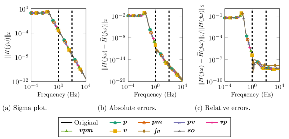
Figure 2: Frequency-limited ROMs for the single chain oscillator (full-order Gramians).

As first example, we consider the single chain oscillator benchmark from [32], where we removed the holonomic constraint to get a mechanical system without algebraic parts. Figure 1 shows the basic setup of the system, where the parameters are chosen as in [32], i.e. in our experiments we have

$$m_{1} =\ldots=m_{n}=100,$$

$$k_{1} =\ldots=k_{n-1}=\kappa_{2}=\ldots=\kappa_{n-1}=2,$$

$$d_{1} =\ldots=d_{n-1}=\delta_{2}=\ldots=\delta_{n-1}=5,$$

and $\kappa_{1}=\kappa_{n}=4$, $\delta_{1}=\delta_{n}=10$. The input and output matrices are chosen to be $B_{u}=e_{1}$ and $C_{p}=[e_{1},e_{2},e_{n-1}]^{\mkern-1.5mu\mathsf{T}}$, where $e_{i}$ denotes the $i$-th column of the identity matrix $I_{n}$. Also, we have chosen $n=12\,000$ masses for the system. This system doe not have any velocity outputs $C_{v}$.

4.1.1 Frequency domain

The frequency range of interest in this example is chosen, just for demonstration reasons, to be between $1$ and $100$ Hz. The computations have been done with no $\alpha$-shift ($\alpha=0$). In Figure 2, the resulting reduced-order models (ROMs) can be seen in terms of their transfer functions (a), the point-wise absolute error (b) and point-wise relative error (c). The frequency range of interest is marked as the area between the dashed vertical lines. Table 3 gives an overview for all applied second-order frequency-limited. It can be noted that all computed ROMs are of order $2$, stable and have absolute and relative errors in the same order of magnitude. Also we note that as wanted, the errors in the frequency range of interest are significantly smaller than in the overall considered frequency region. For the two-step approach, we used, on the one hand, a logarithmically equidistant sampling of $200$ frequency points in the frequency region of interest and, on the other, for a global approximation logarithmically equidistant points between $10^{-4}$ and $10^{4}$ Hz. After a rank truncation of the orthogonalized basis, the intermediate ROMs had the dimension $100$. Since no significant differences between the full-order Gramian and two-step approaches could be seen, we refer the reader also to Figure 2 and Table 3 for the results.

4.1.2 Time domain

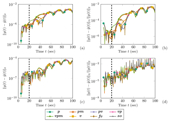
Figure 3: Absolute and relative errors of time-limited ROMs for the single chain oscillator with inputs $u_{\operatorname{step}}$ (a), (b) and $u_{\sin}$ (c), (d) (full-order Gramians).

In the time domain, we apply two different input signals to test our ROMs

$$\begin{aligned} u_{\operatorname{step}}(t)&=\delta(t-5)&&\text{and}&u_{\sin}(t)&=\sin(t)\delta(t-5),\end{aligned}$$ (24)

for $t\in[0,100]$ and $\delta(t)$ the Heaviside function. As time range of interest, $[0,20]$ has been chosen.

While Figure 3 shows the results for the time-limited balanced truncation methods in terms of absolute and relative errors for the two applied input signals (24), in Table 3, the ROM sizes, absolute and relative errors are given. One can observe that all ROMs are of order $4$, stable and have locally significantly smaller errors than globally.

Again, the result of the two-step approaches are only marginal distinguishable from the results of the full-order Gramians, where we used the global sampling between $10^{-4}$ and $10^{4}$ Hz to pre-approximate the system’s behavior. Therefore, those results are also not shown here.

Table 2: Frequency-limited ROMs for the single chain oscillator (full-order Gramians).

	p	pm	pv	vp	vpm	v	fv	so
ROM sizes	2	2	2	2	2	2	2	2
Stability	✓	✓	✓	✓	✓	✓	✓	✓
Global absolute errors	1.011e-01	1.011e-01	1.011e-01	1.011e-01	1.011e-01	1.011e-01	1.012e-01	1.012e-01
Local absolute errors	4.276e-11	4.277e-11	4.276e-11	7.439e-11	7.439e-11	7.439e-11	4.276e-11	7.439e-11
Global relative errors	2.888e-01	2.888e-01	2.888e-01	2.888e-01	2.888e-01	2.888e-01	2.889e-01	2.889e-01
Local relative errors	1.766e-07	1.766e-07	1.766e-07	3.072e-07	3.072e-07	3.072e-07	1.766e-07	3.072e-07

Table 3: Time-limited ROMs for the single chain oscillator (full-order Gramians).

		p	pm	pv	vp	vpm	v	fv	so
ROM sizes		4	4	4	4	4	4	4	4
Stability		✓	✓	✓	✓	✓	✓	✓	✓
$u_{\operatorname{step}}$	Global absolute errors	9.621e-04	1.020e-03	9.619e-04	9.401e-04	9.985e-04	9.393e-04	9.880e-04	9.568e-04
	Local absolute errors	7.953e-07	6.408e-07	7.980e-07	1.456e-06	2.866e-06	1.445e-06	8.597e-07	1.170e-06
	Global relative errors	4.724e-03	5.014e-03	4.723e-03	4.616e-03	4.910e-03	4.611e-03	4.853e-03	4.697e-03
	Local relative errors	4.204e-05	1.256e-05	4.217e-05	4.617e-05	1.384e-05	4.634e-05	4.953e-05	4.503e-05
$u_{\sin}$	Global absolute errors	5.232e-05	5.215e-05	5.231e-05	5.081e-05	5.045e-05	5.079e-05	5.350e-05	5.208e-05
	Local absolute errors	8.600e-07	4.580e-07	8.619e-07	9.591e-07	4.961e-07	9.638e-07	9.471e-07	9.263e-07
	Global relative errors	8.275e-02	8.066e-02	8.273e-02	8.030e-02	7.827e-02	8.026e-02	8.465e-02	8.231e-02
	Local relative errors	3.053e-04	1.150e-04	3.062e-04	3.264e-04	1.261e-04	3.284e-04	3.526e-04	3.214e-04

4.2 Crankshaft

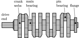
Figure 4: Crankshaft of a four-cylinder engine [35].

The crankshaft is a model from the University Stuttgart, describing the crankshaft of a four-cylinder engine [35], which is shown in Figure 4. After discretization by the finite element method, the constraint model is of dimension $n=42\,126$ with $m=p=35$ inputs and outputs. Due to the rigid elements, coupling the interface nodes, the system has several eigenvalues at zero. Therefore, we apply the shift $\alpha=0.01$, as suggested in Section 3.2, to make the system asymptotically stable during the computations of the matrix equations and low-rank projection matrices.

4.2.1 Frequency domain

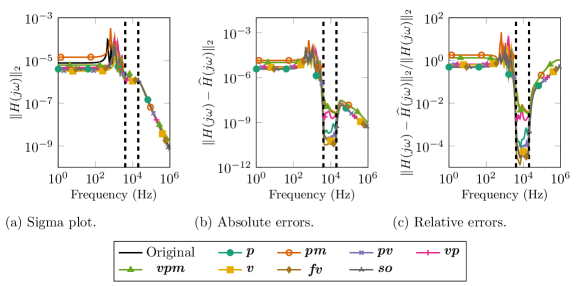
Figure 5: Frequency-limited ROMs for the crankshaft (full-order Gramians).

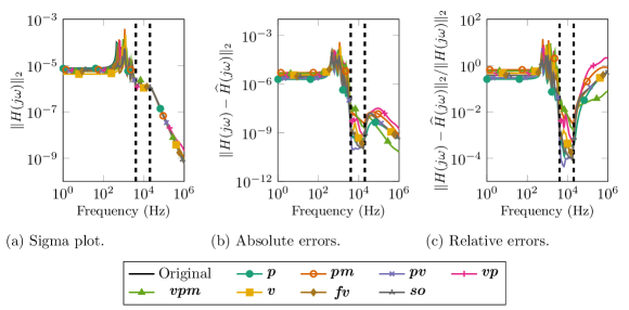
Figure 6: Frequency-limited ROMs for the crankshaft (two-step methods).

In the frequency domain, we are interested in the actual working range of the crankshaft between $4$ and $20$ kHz. Figure 5 shows the results for using the full-order frequency-limited Gramians. The frequency range of interest lies again between the two vertical dashed lines. We can see that all ROMs approximate the frequency region of interest better than the global region. Also Table 5 shows the desired approximation behavior in terms of the errors. In this example, some of the computed ROMs are unstable as denoted by x-marks in Table 5. It should be noted that even for the same order some methods might produce unstable models while others do not.

In this example, we also applied the two-step approach with $200$ frequency sample points in the region of interest to generate the intermediate model of order $447$. Those results can be seen in Figure 6. Table 5 shows that the ROMs produced by the two-step approach are slightly larger in dimension and also partially in errors, while the same methods (pm, vp, vpm, so) as for the full-order Gramian approach produce unstable models.

4.2.2 Time domain

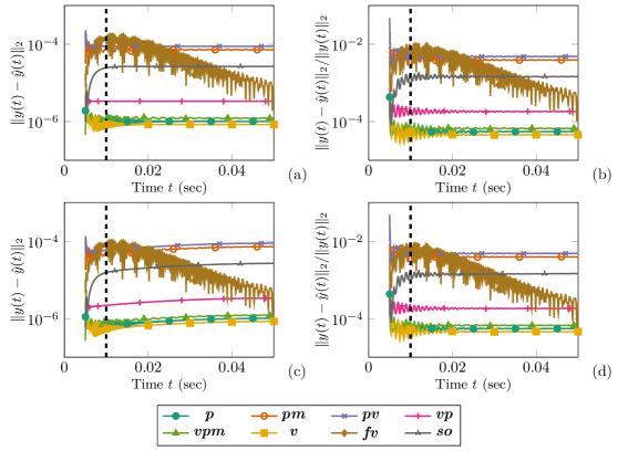
Figure 7: Absolute and relative errors of time-limited ROMs for the crankshaft with inputs $u_{\operatorname{step}}$ (a), (b) and $u_{\sin}$ (c), (d) (full-order Gramians).

In the time domain, we consider just the first $0.01$ s of using the crankshaft, while the full simulation runs over a time range of $[0,0.05]$ s. As test input signals, we apply

$$\begin{aligned} u_{\operatorname{step}}(t)&=3000\delta(t-0.005)\cdot\mathds{1}_{35}&&\text{and}&u_{\sin}(t)&=1500(sin(10\pi t)+1)\delta(t-0.005)\cdot\mathds{1}_{35},\end{aligned}$$

where $\mathds{1}_{35}$ denotes the ones vector of length $35$. The results for the time-limited balanced truncation with the full-order Gramians can be seen in Figure 7 and Table 7. Only one unstable model (vpm) was computed, which still gives suitable approximation results, and all ROMs have small enough errors in the time domain. Even so, we recognize that the local approximation error is only in some cases a bit smaller than the global one.

For the two-step approach, we computed $200$ logarithmically equidistant distributed samples in the frequency domain between $10^{-2}$ and $10^{6}$ Hz. The intermediate model had the order $876$. Since the resulting ROMs are of the same order as the ones computed via the full-order Gramians, featuring the same stability properties, and are only slightly worse in terms of the time domain errors than in Table 7, we skip the additional presentation of those results here.

Table 4: Frequency-limited ROMs for the crankshaft (full-order Gramians).

	p	pm	pv	vp	vpm	v	fv	so
ROM sizes	77	77	65	88	88	69	77	77
Stability	✓	✗	✓	✗	✗	✓	✓	✗
Global absolute errors	9.367e-05	3.237e-04	9.280e-05	1.141e-04	9.601e-05	9.265e-05	9.361e-05	9.345e-05
Local absolute errors	1.588e-09	1.816e-08	9.855e-10	5.497e-09	4.978e-08	4.413e-10	1.011e-10	2.818e-10
Global relative errors	4.627e+00	2.082e+01	2.353e+00	1.439e+01	4.682e+00	4.718e+00	3.963e+00	2.652e+00
Local relative errors	1.327e-03	1.754e-02	8.237e-04	5.117e-03	4.807e-02	4.261e-04	9.759e-05	2.722e-04

Table 5: Frequency-limited ROMs for the crankshaft (two-step methods).

	p	pm	pv	vp	vpm	v	fv	so
ROM sizes	84	84	67	93	93	70	84	70
Stability	✓	✗	✓	✗	✗	✓	✓	✗
Global absolute errors	1.405e-04	3.945e-04	1.026e-04	1.204e-04	1.364e-04	2.138e-04	1.065e-04	9.057e-05
Local absolute errors	2.037e-09	2.569e-08	8.225e-10	7.911e-09	3.709e-08	3.846e-09	1.297e-09	1.774e-09
Global relative errors	2.041e+00	1.400e+01	5.712e+00	7.743e+00	9.187e+00	9.393e+00	3.565e+00	2.865e+00
Local relative errors	1.967e-03	2.481e-02	6.874e-04	7.775e-03	3.462e-02	1.810e-03	1.252e-03	1.713e-03

4.3 Artificial fishtail

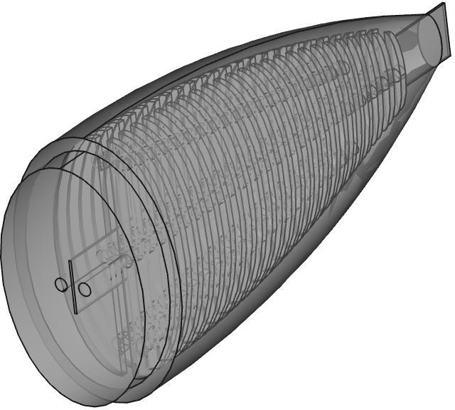
Figure 8: Transparent sketch of the artificial fishtail with embedded fluid chambers.

The artificial fishtail is a mechanical system, describing the movement of a fishtail-shaped structure by using the fluid elastomer actuation principle. Figure 8 shows a transparent sketch of the fishtail model consisting of a carbon beam in the center and a silicon hull around. A more detailed description of the model as well as a comparison of structure-preserving second-order model reduction techniques for this example can be found in [40]. After spatial discretization by the finite element method, the resulting second-order system has $n=779\,232$ states describing the model. By the actuation principle, we have $m=1$ input and a sensor is measuring the displacement of the fishtail’s tip in all spatial dimensions, i.e., we have $p=3$ position outputs and no velocity outputs. The discretized data is available as open benchmark at [43]. The computations were done without an $\alpha$-shift ($\alpha=0$).

4.3.1 Frequency domain

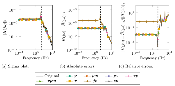
Figure 9: Frequency-limited ROMs for the artificial fishtail (full-order Gramians).

In the frequency domain, the range of interest for the fishtail model lies between $0$ and $20$ Hz, since higher frequencies are physically not realizable. Figure 9 shows the results for the frequency-limited balanced truncation methods, based on the full-order Gramians. Except for the fv balancing there is no visible difference between the ROMs and the full-order model. The error plots show that the approximation reached a sufficiently small error in the region of interest. Table 7 shows the corresponding maximum absolute and relative error in the local and global frequency regions. It is remarkable that the methods were able to approximate the original model, having around $780\,000$ states, by stable order $1$ systems in the region of interest. While the absolute errors are comparable between local and global region, the relative errors show again the strength of the frequency-limited method.

4.3.2 Time domain

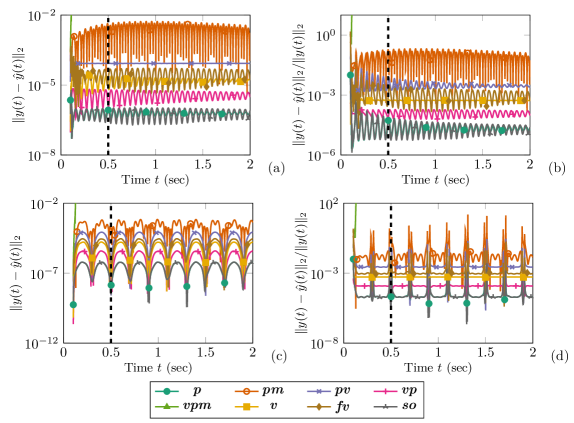
Figure 10: Absolute and relative errors of time-limited ROMs for the artificial fishtail with inputs $u_{\operatorname{step}}$ (a), (b) and $u_{\sin}$ (c), (d) (full-order Gramians).

In the time domain, the fishtail is simulated from $0$ to $2$ s. For our time-limited methods we consider the time range up to $0.5$ s and as inputs, the following two signals are considered

$$\begin{aligned} u_{\operatorname{step}}(t)&=5000\delta(t-0.1)&&\text{and}&u_{\sin}(t)&=2500(sin(10\pi(t-1.35))+1)\delta(t-0.1).\end{aligned}$$

Figure 10 and Table 9 show the results. Except for the models generated by pm, vpm and fv, the computed ROMs have acceptable small errors in the time domain. Also, only the vpm ROM is unstable. The errors in the local region are sometimes a bit smaller than the global one as we were aiming for by the method.

The two-step approach here used $200$ logarithmically equidistant sample points in the frequency range from $10^{-4}$ to $10^{4}$ Hz, which gave an intermediate model of order $100$. The results of the ROMs computed by the two-step approach differ a bit from the ones generated by the full-order Gramians. Those results can be seen in Table 9. There, shown errors are partially smaller or larger than in Table 9 and also we note that for the two-step approach, the vpm model is also unstable but still gives usable results for both applied input signals.

Table 6: Time-limited ROMs for the crankshaft (full-order Gramians).

		p	pm	pv	vp	vpm	v	fv	so
ROM sizes		58	58	37	132	132	59	58	59
Stability		✓	✓	✓	✓	✗	✓	✓	✓
$u_{\operatorname{step}}$	Global absolute errors	9.442e-06	8.765e-05	2.331e-04	4.771e-06	1.567e-06	7.733e-06	1.884e-04	2.669e-05
	Local absolute errors	9.442e-06	8.765e-05	2.331e-04	4.771e-06	1.567e-06	7.733e-06	1.554e-04	2.467e-05
	Global relative errors	5.573e-04	8.707e-03	4.803e-02	7.460e-04	1.039e-04	4.103e-04	1.078e-02	1.731e-03
	Local relative errors	5.573e-04	8.707e-03	4.803e-02	7.460e-04	1.039e-04	4.103e-04	9.845e-03	1.731e-03
$u_{\sin}$	Global absolute errors	5.459e-06	7.231e-05	1.349e-04	3.345e-06	1.233e-06	4.472e-06	1.089e-04	2.664e-05
	Local absolute errors	5.459e-06	5.245e-05	1.349e-04	2.760e-06	9.133e-07	4.472e-06	8.980e-05	1.547e-05
	Global relative errors	5.559e-04	8.707e-03	4.803e-02	7.460e-04	1.028e-04	4.103e-04	9.189e-03	1.610e-03
	Local relative errors	5.559e-04	8.707e-03	4.803e-02	7.460e-04	1.028e-04	4.103e-04	8.605e-03	1.610e-03

Table 7: Frequency-limited ROMs for the artificial fishtail (full-order Gramians).

	p	pm	pv	vp	vpm	v	fv	so
ROM sizes	1	1	1	1	1	1	1	1
Stability	✓	✓	✓	✓	✓	✓	✓	✓
Global absolute errors	4.409e-07	4.409e-07	4.409e-07	4.409e-07	4.409e-07	4.409e-07	1.172e-04	4.409e-07
Local absolute errors	1.046e-07	1.538e-07	1.043e-07	8.975e-08	1.558e-07	8.964e-08	1.172e-04	1.045e-07
Global relative errors	9.182e+00	9.176e+00	9.182e+00	9.181e+00	9.174e+00	9.181e+00	1.596e+01	9.182e+00
Local relative errors	1.132e-02	1.200e-02	1.132e-02	1.150e-02	1.219e-02	1.150e-02	9.557e-01	1.132e-02

Table 8: Time-limited ROMs for the artificial fishtail (full-order Gramians).

		p	pm	pv	vp	vpm	v	fv	so
ROM sizes		4	4	2	6	6	4	4	4
Stability		✓	✓	✓	✓	✗	✓	✓	✓
$u_{\operatorname{step}}$	Global absolute errors	5.523e-06	5.277e-03	2.320e-04	7.032e-06	$\infty$	3.049e-05	4.650e-04	6.087e-06
	Local absolute errors	5.523e-06	4.282e-03	2.320e-04	7.032e-06	$\infty$	3.049e-05	4.650e-04	6.087e-06
	Global relative errors	9.961e-03	4.577e-01	1.524e-01	4.127e-04	$\infty$	2.799e-03	1.489e+00	8.162e-03
	Local relative errors	9.961e-03	4.577e-01	1.524e-01	4.127e-04	$\infty$	2.799e-03	1.489e+00	8.162e-03
$u_{\sin}$	Global absolute errors	6.103e-07	6.845e-04	8.434e-05	3.878e-06	$\infty$	1.681e-05	2.898e-05	6.237e-07
	Local absolute errors	6.094e-07	6.278e-04	8.434e-05	3.850e-06	$\infty$	1.681e-05	2.846e-05	6.129e-07
	Global relative errors	9.961e-03	1.525e+01	2.819e-01	6.047e-03	$\infty$	3.089e-03	1.489e+00	8.162e-03
	Local relative errors	9.961e-03	1.549e+00	1.224e-01	8.350e-04	$\infty$	1.192e-03	1.489e+00	8.162e-03

Table 9: Time-limited ROMs for the artificial fishtail (two-step methods).

		p	pm	pv	vp	vpm	v	fv	so
ROM sizes		4	4	2	9	9	4	4	4
Stability		✓	✓	✓	✓	✗	✓	✓	✓
$u_{\operatorname{step}}$	Global absolute errors	5.506e-06	1.306e-03	2.308e-04	6.210e-06	1.394e-03	6.649e-05	2.229e-04	7.206e-06
	Local absolute errors	5.506e-06	1.306e-03	2.308e-04	6.210e-06	1.137e-03	6.649e-05	2.229e-04	7.206e-06
	Global relative errors	1.088e-02	2.335e+00	1.517e-01	2.461e-03	2.321e-01	2.253e-02	9.866e-01	4.656e-03
	Local relative errors	1.088e-02	2.335e+00	1.517e-01	2.461e-03	2.321e-01	2.253e-02	9.866e-01	4.656e-03
$u_{\sin}$	Global absolute errors	9.836e-07	9.156e-04	8.371e-05	5.547e-07	3.619e-04	2.309e-05	9.389e-07	9.808e-07
	Local absolute errors	9.885e-07	9.156e-04	8.371e-05	5.560e-07	3.887e-04	2.316e-05	9.389e-07	9.899e-07
	Global relative errors	1.088e-02	2.335e+00	2.775e-01	2.613e-03	4.312e+00	1.152e-01	9.866e-01	4.656e-03
	Local relative errors	1.088e-02	2.335e+00	1.218e-01	1.585e-03	6.518e-01	3.076e-02	9.866e-01	4.656e-03

5 Conclusions

We extended the frequency- and time-limited balanced truncation methods from first-order systems to the second-order case by applying the different second-order balancing approaches from the literature. For the application of the introduced theory, we investigated numerical methods for approximating the solution of the arising large-scale sparse matrix equations with function right hand-sides as well as techniques to deal with the difficulties arising from the second-order system structure. The numerical examples show that the methods work for the purpose of limited model reduction in the frequency domain and also for some examples in time domain. By comparison of the different balancing formulas, it was not possible to determine a clear winner or loser. Depending on the example, different balancing techniques performed better or worse than the others. Also, stability preservation is still an open problem for this type of model reduction techniques, where we pointed out that the known modifications from the first-order case are not necessarily stability preserving for second-order systems.

References

- [1] J. Baker, M. Embree, and J. Sabino. Fast singular value decay for Lyapunov solutions with nonnormal coefficients. SIAM J. Matrix Anal. Appl., 36(2):656–668, 2015. doi:10.1137/140993867.
- [2] C. A. Beattie and S. Gugercin. Krylov-based model reduction of second-order systems with proportional damping. In Proceedings of the 44th IEEE Conference on Decision and Control, pages 2278–2283, December 2005. doi:10.1109/CDC.2005.1582501.
- [3] P. Benner, J. M. Claver, and E. S. Quintana-Ortí. Efficient solution of coupled Lyapunov equations via matrix sign function iteration. In Proc. Portuguese Conf. on Automatic Control CONTROLO’98, Coimbra, pages 205–210, 1998.
- [4] P. Benner, P. Kürschner, and J. Saak. A reformulated low-rank ADI iteration with explicit residual factors. Proc. Appl. Math. Mech., 13(1):585–586, 2013. doi:10.1002/pamm.201310273.
- [5] P. Benner, P. Kürschner, and J. Saak. Self-generating and efficient shift parameters in ADI methods for large Lyapunov and Sylvester equations. Electron. Trans. Numer. Anal., 43:142–162, 2014.
- [6] P. Benner, P. Kürschner, and J. Saak. Frequency-limited balanced truncation with low-rank approximations. SIAM J. Sci. Comput., 38(1):A471–A499, February 2016. doi:10.1137/15M1030911.
- [7] P. Benner, P. Kürschner, Z. Tomljanović, and N. Truhar. Semi-active damping optimization of vibrational systems using the parametric dominant pole algorithm. Z. Angew. Math. Mech., 96(5):604–619, 2016. doi:10.1002/zamm.201400158.
- [8] P. Benner, J.-R. Li, and T. Penzl. Numerical solution of large-scale Lyapunov equations, Riccati equations, and linear-quadratic optimal control problems. 15(9):755–777, 2008. doi:10.1002/nla.622.
- [9] P. Benner, E. S. Quintana-Ortí, and G. Quintana-Ortí. Balanced truncation model reduction of large-scale dense systems on parallel computers. Math. Comput. Model. Dyn. Syst., 6(4):383–405, 2000. doi:10.1076/mcmd.6.4.383.3658.
- [10] P. Benner and J. Saak. Numerical solution of large and sparse continuous time algebraic matrix Riccati and Lyapunov equations: a state of the art survey. GAMM Mitteilungen, 36(1):32–52, August 2013. doi:10.1002/gamm.201310003.
- [11] P. Benner and T. Stykel. Model order reduction for differential-algebraic equations: A survey. In Achim Ilchmann and Timo Reis, editors, Surveys in Differential-Algebraic Equations IV, Differential-Algebraic Equations Forum, pages 107–160. Springer International Publishing, Cham, March 2017. doi:10.1007/978-3-319-46618-7\_3.
- [12] P. Benner and S. W. R. Werner. MORLAB – Model Order Reduction LABoratory (version 5.0), 2019. see also: http://www.mpi-magdeburg.mpg.de/projects/morlab. doi:10.5281/zenodo.3332716.
- [13] P. Benner and S. W. R. Werner. Limited balanced truncation for large-scale sparse second-order systems (version 2.0), 2020. doi:10.5281/zenodo.3331592.
- [14] T. Breiten. Structure-preserving model reduction for integro-differential equations. SIAM J. Control Optim., 54(6):2992–3015, 2016. doi:10.1137/15M1032296.
- [15] V. Chahlaoui, K. A. Gallivan, A. Vandendorpe, and P. Van Dooren. Model reduction of second-order system. In P. Benner, V. Mehrmann, and D. C. Sorensen, editors, Dimension Reduction of Large-Scale Systems, volume 45 of Lect. Notes Comput. Sci. Eng., pages 149–172. Springer-Verlag, Berlin/Heidelberg, Germany, 2005. doi:10.1007/3-540-27909-1_6.
- [16] Y. Chahlaoui, D. Lemonnier, A. Vandendorpe, and P. Van Dooren. Second-order balanced truncation. Linear Algebra Appl., 415(2–3):373–384, 2006. doi:10.1016/j.laa.2004.03.032.
- [17] V. Druskin and V. Simoncini. Adaptive rational Krylov subspaces for large-scale dynamical systems. Syst. Cont. Lett., 60(8):546–560, 2011. doi:10.1016/j.sysconle.2011.04.013.
- [18] J. Fehr and P. Eberhard. Error-controlled model reduction in flexible multibody dynamics. J. Comput. Nonlinear Dynam., 5(3):031005–1–031005–8, 2010. doi:10.1115/1.4001372.
- [19] F. Freitas, J. Rommes, and N. Martins. Gramian-based reduction method applied to large sparse power system descriptor models. IEEE Trans. Power Syst., 23(3):1258–1270, August 2008. doi:10.1109/TPWRS.2008.926693.
- [20] W. Gawronski and J.-N. Juang. Model reduction in limited time and frequency intervals. Int. J. Syst. Sci., 21(2):349–376, 1990. doi:10.1080/00207729008910366.
- [21] S. Gugercin and A. C. Antoulas. A survey of model reduction by balanced truncation and some new results. Internat. J. Control, 77(8):748–766, 2004. doi:10.1080/00207170410001713448.
- [22] K. Haider, A. Ghafoor, M. Imran, and F. M. Malik. Model reduction of large scale descriptor systems using time limited Gramians. Asian J. Control, 19(3):1217–1227, 2017. doi:10.1002/asjc.1444.
- [23] K. Haider, A. Ghafoor, M. Imran, and F. M. Malik. Frequency interval Gramians based structure preserving model reduction for second-order systems. Asian J. Control, 20(2):790–801, 2018. doi:10.1002/asjc.1598.
- [24] K. Haider, A. Ghafoor, M. Imran, and F. M. Malik. Time-limited Gramian-based model order reduction for second-order form systems. Transactions of the Institute of Measurement and Control, 00(0):1–9, 2018. doi:10.1177/0142331218798893.
- [25] N. J. Higham. Functions of Matrices: Theory and Computation. Applied Mathematics. SIAM Publications, Philadelphia, PA, 2008. doi:10.1137/1.9780898717778.
- [26] M. Imran and A. Ghafoor. Model reduction of descriptor systems using frequency limited Gramians. J. Franklin Inst., 352(1):33–51, 2015. doi:10.1016/j.jfranklin.2014.10.013.
- [27] I. M. Jaimoukha and E. M. Kasenally. Krylov subspace methods for solving large Lyapunov equations. SIAM J. Numer. Anal., 31(1):227–251, 1994. doi:10.1137/0731012.
- [28] P. Kürschner. Balanced truncation model order reduction in limited time intervals for large systems. Advances in Computational Mathematics, 44(6):1821–1844, 2018. doi:10.1007/s10444-018-9608-6.
- [29] N. Lang, H. Mena, and J. Saak. On the benefits of the factorization for large-scale differential matrix equation solvers. Linear Algebra Appl., 480:44–71, September 2015. doi:10.1016/j.laa.2015.04.006.
- [30] M. Lehner and P. Eberhard. A two-step approach for model reduction in flexible multibody dynamics. Multibody Syst. Dyn., 17(2-3):157–176, 2007. doi:10.1007/s11044-007-9039-5.
- [31] J.-R. Li and J. White. Low rank solution of Lyapunov equations. SIAM J. Matrix Anal. Appl., 24(1):260–280, 2002. doi:10.1137/S0895479801384937.
- [32] V. Mehrmann and T. Stykel. Balanced truncation model reduction for large-scale systems in descriptor form. In P. Benner, V. Mehrmann, and D. C. Sorensen, editors, Dimension Reduction of Large-Scale Systems, volume 45 of Lect. Notes Comput. Sci. Eng., pages 83–115. Springer-Verlag, Berlin/Heidelberg, Germany, 2005. doi:10.1007/3-540-27909-1_3.
- [33] D. G. Meyer and S. Srinivasan. Balancing and model reduction for second-order form linear systems. IEEE Trans. Autom. Control, 41(11):1632–1644, 1996. doi:10.1109/9.544000.
- [34] B. C. Moore. Principal component analysis in linear systems: controllability, observability, and model reduction. IEEE Trans. Autom. Control, AC–26(1):17–32, 1981. doi:10.1109/TAC.1981.1102568.
- [35] C. Nowakowski, P. Kürschner, P. Eberhard, and P. Benner. Model reduction of an elastic crankshaft for elastic multibody simulations. Z. Angew. Math. Mech., 93:198–216, 2013. doi:10.1002/zamm.201200054.
- [36] H. Panzer, T. Wolf, and B. Lohamnn. A strictly dissipative state space representation of second order systems. at-Automatisierungstechnik, 60(7):392–397, 2012. doi:10.1524/auto.2012.1015.
- [37] T. Reis and T. Stykel. Balanced truncation model reduction of second-order systems. Math. Comput. Model. Dyn. Syst., 14(5):391–406, 2008. doi:10.1080/13873950701844170.
- [38] J. Rommes and N. Martins. Computing transfer function dominant poles of large-scale second-order dynamical systems. IEEE Trans. Power Syst., 21(4):1471–1483, November 2006. doi:10.1109/TPWRS.2006.881154.
- [39] J. Saak, M. Köhler, and P. Benner. M-M.E.S.S.-2.0 – the matrix equations sparse solvers library, August 2019. see also: https://www.mpi-magdeburg.mpg.de/projects/mess. doi:10.5281/zenodo.3368844.
- [40] J. Saak, D. Siebelts, and S. W. R. Werner. A comparison of second-order model order reduction methods for an artificial fishtail. at-Automatisierungstechnik, 67(8):648–667, 2019. doi:10.1515/auto-2019-0027.
- [41] B. Salimbahrami. Structure Preserving Order Reduction of Large Scale Second Order Models. Dissertation, Technische Universität München, Munich, Germany, 2005. URL: https://mediatum.ub.tum.de/doc/601950/00000941.pdf.
- [42] B. Salimbahrami and B. Lohmann. Order reduction of large scale second-order systems using Krylov subspace methods. Linear Algebra Appl., 415(2–3):385–405, 2006. doi:10.1016/j.laa.2004.12.013.
- [43] D. Siebelts, A. Kater, T. Meurer, and J. Andrej. Matrices for an artificial fishtail. hosted at MORwiki – Model Order Reduction Wiki, 2019. doi:10.5281/zenodo.2558728.
- [44] V. Simoncini. A new iterative method for solving large-scale Lyapunov matrix equations. SIAM J. Sci. Comput., 29(3):1268–1288, 2007. doi:10.1137/06066120X.
- [45] T. Stykel. Analysis and Numerical Solution of Generalized Lyapunov Equations. Dissertation, TU Berlin, 2002. URL: http://webdoc.sub.gwdg.de/ebook/e/2003/tu-berlin/stykel_tatjana.pdf.
- [46] T. Wolf, H. K. F. Panzer, and B. Lohmann. Model order reduction by approximate balanced truncation: A unifying framework. at-Automatisierungstechnik, 61(8):545–556, 2013. doi:10.1524/auto.2013.1007.
- [47] S. Wyatt. Issues in Interpolatory Model Reduction: Inexact Solves, Second Order Systems and DAEs. PhD thesis, Virginia Polytechnic Institute and State University, Blacksburg, Virginia, USA, May 2012. URL: https://vtechworks.lib.vt.edu/bitstream/handle/10919/27668/Wyatt_SA_D_2012.pdf?sequence=1.