Theory of Higgs Modes in $d$-Wave Superconductors

Abstract

By applying a microscopic gauge-invariant kinetic theory in $d$-wave superconductors, we analytically derive the energy spectra of the breathing Higgs mode and, in particular, rotating Higgs mode that is unique for the $d$-wave order parameter. Analytical investigation on their dynamic properties is also revealed. We show that the breathing Higgs mode is optically visible in the second-order regime. Whereas the rotating Higgs mode is optically inactive, we show that this mode can be detected in the pseudogap phase by magnetic resonance experiment. It is interesting to find that with a longitudinal temperature gradient, the charge-neutral rotating Higgs mode generates a thermal Hall current by magnetic field in the pseudogap phase, providing a unique scheme for its detection.

Introduction.—In the past few decades, collective excitation in the field of superconductivity has attracted much attention. Due to the angular and radial excitations in the Mexican-hat potential of free energy Am0 , two types of the collective excitations emerge: Nambu-Goldstone gi0 ; AK ; Gm1 ; Gm2 ; Ba0 ; pi1 and Higgs OD1 ; OD2 ; OD3 ; Am12 modes, which describe the phase and amplitude fluctuations of the superconducting order parameter respectively. These modes are decoupled in equilibrium state as they represent mutually orthogonal excitations Am0 . The Nambu-Goldstone mode corresponds to gapless Goldstone boson due to the spontaneous breaking of continuous $U(1)$ symmetry by order parameter Gm1 ; Gm2 . For the Higgs mode, theoretical studies in conventional $s$-wave superconductors reveal an excitation gap at long wavelength, twice of the superconducting gap Am0 ; OD1 . Whereas being charge neutral and spinless, this mode has long been experimentally elusive. Until recently, thanks to advanced ultrafast terahertz pump-probe technique, the Higgs mode in conventional superconductors has been observed from the optically excited oscillation of the superfluid density in second-order regime NL1 ; NL2 ; NL3 ; NL4 . The most convincing evidence comes from the triggered resonance at the optical frequency which equals to superconducting gap NL2 ; NL3 ; NL4 . The Higgs mode has since stimulated a lot of experimental interest in a variety of contexts, extending to unconventional superconductors. Particularly, recent experiments in cuprate superconductor reported similar oscillation of superfluid density in the second-order optical response DHM1 ; DHM2 ; DHM3 , indicating the observation of the Higgs mode in high-$T_{c}$ superconductors.

Despite experimental activity, the theoretical description of the Higgs mode in high-$T_{c}$ superconductors remains wide open DHMT1 ; DHMT2 . In high-$T_{c}$ superconductors, a finite amplitude of the order parameter persists up to $T^{*}$, which is well above $T_{c}$ PG1 ; PG2 ; PG3 ; PG4 ; PG5 , indicating the existence of the Higgs mode not only in superconducting phase but also in pseudogap one. Moreover, compared with the $s$-wave case, the high-$T_{c}$ superconductivity with the $d$-wave order parameter and hence the lower rotating symmetry supports the additional Higgs modes. Early symmetry analysis revealed the existence of the breathing and rotating Higgs modes DHMT1 , which for the case of $d_{x^{2}-y^{2}}$-wave order parameter correspond to $d_{x^{2}-y^{2}}$-wave and $d_{xy}$-wave amplitude fluctuations, respectively. The breathing Higgs mode is expected to be similar to conventional $s$-wave Higgs mode, whereas the rotating one is unique. Recent experiment in cuprate superconductor has reported that the direction of the order parameter detaches from that of lattice Ro . A detectable response of rotating Higgs mode to the external probe is therefore expected. Nevertheless, the energy spectra and dynamic properties for both Higgs modes in $d$-wave superconductors are still unclear in the literature. Considering the growing experimental findings, a full theoretical investigation on these modes becomes imperative.

In this Letter, we use the microscopic gauge-invariant kinetic equation (GIKE) approach GOBE1 ; GOBE2 to investigate the Higgs modes for $d$-wave order parameter. For the first time, we provide the analytic expressions for energy spectra of both breathing and rotating Higgs modes. Then, investigation on their dynamic properties is presented. The breathing Higgs mode is optically visible in the second-order regime, irrelevant of the optical polarization direction. Whereas the rotating Higgs mode is optically inactive, we show that this mode responds to magnetic field in the linear regime, suggesting a possible detection by magnetic resonance experiment in the pseudogap phase. It is interesting to find that the charge-neutral rotating Higgs mode, which does not manifest itself in the electric measurement, generates a thermal Hall current by magnetic field in the presence of temperature gradient in pseudogap phase, providing a unique scheme for its detection.

Hamiltonian.—We begin our analysis with a free two-dimensional BCS-like Hamiltonian

$$H=\sum_{{\bf k},s=\uparrow,\downarrow}\xi_{\bf k}c^{\dagger}_{{\bf k}s}c_{{\bf k}s}-\sum_{{\bf kk^{\prime}}}g_{\bf kk^{\prime}}c^{\dagger}_{{\bf k}\uparrow}c^{\dagger}_{-{\bf k}\downarrow}c_{-{\bf k^{\prime}}\downarrow}c_{{\bf k^{\prime}}\uparrow},$$ (1)

where $\xi_{k}=\varepsilon_{k}-\mu$ and $\varepsilon_{k}={k^{2}}/{(2m)}$ with $m$ and $\mu$ being the effective mass and chemical potential, respectively; $g_{\bf kk^{\prime}}$ denotes the pairing interaction. The order parameter is determined by $\Delta_{{\bf k}0}=-\sum_{\bf k^{\prime}}g_{\bf kk^{\prime}}\langle{c_{-{\bf k^{\prime}}\downarrow}c_{{\bf k^{\prime}}\uparrow}}\rangle$. This leads to the Bogoliubov quasiparticle energy $E_{\bf k}=\sqrt{\xi_{k}^{2}+\Delta^{2}_{{\bf k}0}}$. In the present analysis, we approximately take the pairing interaction $g_{\bf kk^{\prime}}$ around the Fermi surface (i.e., $k=k^{\prime}=k_{F}$) so that the order parameter only has angular dependence of the momentum. In the presence of the translational and time-reversal symmetries SM1 , the pairing interaction $g_{\bf kk^{\prime}}=\sum_{m=0}D_{m}\cos{m}(\theta_{\bf k}-\theta_{\bf k^{\prime}})$ where $\theta_{\bf k}$ denotes the angle of ${\bf k}$ vector. For $d$-wave superconductivity, $D_{2}$ channel dominates, i.e.,

$$g_{\bf kk^{\prime}}{\approx}D_{2}\cos{2}(\theta_{\bf k}-\theta_{\bf k^{\prime}}).$$ (2)

However, $g_{\bf kk^{\prime}}$ here exhibits the rotational symmetry of the polar axis in momentum space, and thus, can not determine the direction of the order parameter. This direction, as recent experiment reported Ro , also detaches from that of lattice. The practical formation of the $d$-wave order parameter with a certain direction thus spontaneously breaks the rotational symmetry. Without losing generality, we choose $d_{x^{2}-y^{2}}$ order parameter for analysis, i.e., $\Delta_{{\bf k}0}=\Delta_{0}\cos 2\theta_{\bf k}$. As this finite order parameter in high-$T_{c}$ superconductors persists up to $T^{*}$, which is well above $T_{c}$ PG1 ; PG2 ; PG3 ; PG4 ; PG5 , our calculation of its amplitude fluctuation in the following can be applied not only in superconducting phase but also in pseudogap one.

GIKE approach.—To calculate the Higgs mode, we use the GIKE approach GOBE1 ; GOBE2 , which has been successfully applied to study collective modes and their electromagnetic properties in conventional superconductors GOBE2 . In this microscopic approach, the response of system is described by density matrix $\rho_{\bf k}=\rho^{(0)}_{\bf k}+\delta\rho_{\bf k}(R)$ in Nambu space, which consists of the equilibrium part $\rho^{(0)}_{\bf k}=\frac{1}{2}-\frac{1-2f(E_{\bf k})}{2}(\frac{\xi_{k}}{E_{\bf k}}\tau_{3}+\frac{\Delta_{{\bf k}0}}{E_{\bf k}}\tau_{1})$ and nonequilibrium one $\delta\rho_{\bf k}(R)$. Here, $f(x)=\frac{1}{e^{x/T}+1}$ denotes the Fermi-distribution function with $T$ being the temperature; $\tau_{i}$ are Pauli matrices in particle-hole space; $R=(t,{\bf R})$ represents the center-of-mass (CM) coordinate. The off-diagonal components of $\rho_{\bf k}$ self-consistently determine the order parameter:

$${\hat{\Delta}_{\bf k}({R})} = [\Delta_{{\bf k}0}+\delta\Delta_{\bf k}(R)]e^{i\delta\theta(R)}\tau_{+}+h.c.$$ (3)

$$= -\sum_{\bf k^{\prime}}g_{\bf kk^{\prime}}(\rho_{{\bf k^{\prime}}+}\tau_{+}+h.c.),$$

where $\rho_{{\bf k}i}$ stands for the $\tau_{i}$ component of $\rho_{\bf k}$; $\delta\Delta_{\bf k}$ and $\delta\theta$ denote the amplitude and phase fluctuations of the order parameter, respectively.

To determine the nonequilibrium property/fluctuation, one needs to solve $\delta\rho_{\bf k}$ from the GIKE

$$\partial_{t}\rho_{\bf k}+\partial_{t}\rho_{\bf k}\big{|}_{\rm coh}+\partial_{t}\rho_{\bf k}\big{|}_{\rm diff}+\partial_{t}\rho_{\bf k}\big{|}_{\rm dri}=\partial_{t}\rho_{\bf k}\big{|}_{\rm scat}.$$ (4)

The coherent terms are given by

where $\phi$ and ${\bf A}$ stand for the scalar and vector potentials, respectively; $\mu_{H}(R)=\sum_{\bf R^{\prime}}V_{{\bf R}-{\bf R^{\prime}}}{\delta}n({R}^{\prime})$ describes the induced scalar potential by the density fluctuation ${\delta}n({R}^{\prime})$, with $V_{\bf R-R^{\prime}}$ being the Coulomb potential.

The drive terms by electromagnetic fields read

$$\partial_{t}\rho_{\bf k}\big{|}_{\rm dri}=\leavevmode\resizebox{14.09207pt}{}{$\frac{1}{2}$}\{e{\bf E}\tau_{3}-({\bm{\nabla}}_{\bf R}\!-\!2ie{\bf A}\tau_{3}){{\hat{\Delta}}_{\bf k}(R)},\partial_{\bf k}\rho_{\bf k}\}$$

$$\mbox{}\!-\!\leavevmode\resizebox{15.50415pt}{}{$\frac{i}{8}$}[({\bm{\nabla}_{\bf R}}\!-\!2ie{\bf A}\tau_{3})({\bm{\nabla}_{\bf R}}\!-\!2ie{\bf A}\tau_{3}){\hat{\Delta}}_{\bf k}(R),\partial_{\bf k}\partial_{\bf k}\rho_{\bf k}]$$

$$\mbox{}\!+\!\leavevmode\resizebox{58.71936pt}{}{$\frac{{\bf k}\times{e}{\bf B}}{4m}$}[\tau_{3},\tau_{3}\partial_{\bf k}\rho_{\bf k}]\!+\!\leavevmode\resizebox{56.3683pt}{}{$\frac{{\bf k}\times{e}{\bf B}}{2m}$}\{\tau_{3},\tau_{3}\partial_{\bf k}\rho_{\bf k}\},$$ (6)

with the electric field $e{\bf E}=-{\bm{\nabla}}_{\bf R}(e\phi+\mu_{H})-\partial_{t}e{\bf A}$ and magnetic field ${\bf B}={\bm{\nabla}}_{\bf R}\times{\bf A}$. By the Meissner effect, the magnetic field ${\bf B}$ is expelled from superconductor in superconducting phase. Whereas in pseudogap phase where the superfluid density vanishes, ${\bf B}$ can be applied. Here, we consider a perpendicular ${\bf B}$ to the conducting layer.

The diffusion terms due to spatial inhomogeneity read

$$\partial_{t}\leavevmode\resizebox{46.97836pt}{}{$\rho_{\bf k}\big{|}_{\rm diff}$}\!=\!\{\leavevmode\resizebox{28.18414pt}{}{$\frac{\bf k}{2m}$}\tau_{3},\leavevmode\resizebox{21.1381pt}{}{${\bm{\nabla}}_{\bf R}$}\leavevmode\resizebox{18.78703pt}{}{$\rho_{\bf k}$}\}\!-e[\leavevmode\resizebox{46.97836pt}{}{$\frac{{\nabla_{\bf R}}\circ{\bf A}}{4m}$},\tau_{3}\leavevmode\resizebox{18.78703pt}{}{$\rho_{\bf k}$}]\!-\!\leavevmode\resizebox{13.15308pt}{}{$\frac{i}{4}$}[\varepsilon_{\leavevmode\resizebox{16.44313pt}{}{${\bm{\nabla}_{\bf R}}$}}\tau_{3},\leavevmode\resizebox{18.78703pt}{}{$\rho_{\bf k}$}],$$ (7)

with ${\nabla_{\bf R}}\!\circ\!{\bf A}=(2{\bf A}\!\cdot\!{\bm{\nabla}}_{\bf R}\!+\!{\bm{\nabla}}_{\bf R}\!\cdot\!{\bf A})\tau_{3}$. The lengthy scattering terms $\partial_{t}\rho_{\bf k}|_{\rm scat}$ are presented in the Supplemental Material [see Eq. (S7) SM ].

Calculation of Higgs modes.—The phase fluctuation in Eq. (3) enlarges the difficulty to solve $\delta\rho_{\bf k}$ from Eq. (4), but it can be effectively removed by unitary transformation $\rho_{\bf k}(R)\rightarrow{e^{i\tau_{3}\delta\theta(R)/2}}\rho_{\bf k}(R)e^{-i\tau_{3}\delta\theta(R)/2}$ [see Supplemental Material, Eq. (S3) SM ]. Then, for weak probe, by expanding $\delta\rho_{\bf k}=\delta\rho^{(1)}_{\bf k}+\delta\rho^{(2)}_{\bf k}$ with $\delta\rho^{(1)}_{\bf k}$ and $\delta\rho^{(2)}_{\bf k}$ being the first and second order responses to external probe, the GIKE becomes a chain of equations, as its first order only involves $\delta\rho^{(1)}_{\bf k}$ and equilibrium $\rho^{(0)}_{\bf k}$ and its second order involves $\delta\rho^{(2)}_{\bf k}$, $\delta\rho^{(1)}_{\bf k}$ and $\rho^{(0)}_{\bf k}$. Consequently, starting from the lowest order, we calculate $\delta\rho^{(1)}_{\bf k}$ and $\delta\rho^{(2)}_{\bf k}$ in sequence, whose lengthy expressions are presented in the Supplemental Material [see Eqs. (S16) and (S28) SM ].

Then, we can finally determine the Higgs modes. Particularly, Eq. (3) after above unitary transformation has variation $\Delta_{{\bf k}0}\!+\!\delta\Delta_{\bf k}\!=\!-\sum_{\bf k^{\prime}}g_{\bf kk^{\prime}}\rho_{{\bf k^{\prime}}1}$, from which by the solved $\delta\rho_{\bf k}$ we can self-consistently obtain Higgs mode

$$\delta\Delta_{\bf k}=-\sum_{\bf k^{\prime}}g_{\bf kk^{\prime}}\delta\rho_{{\bf k^{\prime}}1}.$$ (8)

By further considering $g_{\bf kk^{\prime}}$ in Eq. (2), the Higgs mode

$$\delta\Delta_{\bf k}(R)=\delta\Delta_{B}(R)\cos(2\theta_{\bf k})+\delta\Delta_{R}(R)\sin(2\theta_{\bf k}),$$ (9)

consists of breathing $\delta\Delta_{B}(R)$ and rotating $\delta\Delta_{R}(R)$ parts.

Breathing Higgs mode.—In CM frequency and momentum space [$R=(t,{\bf R})\rightarrow{q}=(\omega,{\bf q})$], we find the optical response of the breathing Higgs mode at weak scattering (for details, see Supplemental Material SM )

$$\left(\omega^{2}_{B}-\omega^{2}\right)\delta\Delta_{B}(q)=\Big{(}\frac{e{\bf E}_{q}\cdot{i}{\bf q}}{m}\Big{)}{8u_{\omega}\Delta_{0}}+v^{2}_{F}\left[\frac{2}{i\omega_{\rm H}}{\overline{\Big{(}\frac{e{\bf E}_{q}}{i\omega_{\rm P}}\Big{)}\cdot{e}{\bf E}_{q}}}+2\overline{\Big{(}\frac{e{\bf E}_{q}}{i\omega_{\rm P}}\Big{)}\cdot{e}{\bf A}_{q}}+e^{2}\overline{{\bf A}^{2}_{q}}\right]\Delta_{0}d_{\omega},$$ (10)

where ${\overline{A_{q}B_{q}}}=\int{dq^{\prime}}A_{q^{\prime}}B_{q-q^{\prime}}$; $i\omega_{\rm P}=i\omega+\Gamma_{p}$ and $i\omega_{\rm H}=i\omega+\Gamma_{H}$, with $\Gamma_{p}$ ($\Gamma_{H}$) being the relaxation rate of nonequilibrium $\delta\rho_{{\bf k}0}$ ($\delta\rho_{{\bf k}\pm}$) from the scattering; the energy spectrum

$$\leavevmode\resizebox{272.45874pt}{}{$\omega_{B}=2\Delta_{0}\sqrt{\frac{\sum_{\bf k}\cos^{4}(2\theta_{\bf k})a_{\bf k}z_{\omega_{B},{\bf k}}}{\sum_{\bf k}\cos^{2}(2\theta_{\bf k})a_{\bf k}z_{\omega_{B},{\bf k}}}}$},$$ (11)

with $a_{\bf k}=\frac{1-f(E_{\bf k})}{2E_{\bf k}}$ and $z_{\omega,{\bf k}}=\frac{1}{4E_{\bf k}^{2}-\omega^{2}}$; $u_{\omega}$ and $d_{\omega}$ are the dimensionless coefficients for the linear and second-order responses [see Supplemental Material, Eqs. (S31) and (S32) SM ], respectively.

In this response function, it is first noted from the left-hand side that due to the lower rotational symmetry for the $d$-wave order parameter [i.e., $\cos^{4}(2\theta_{\bf k})\leq\cos^{2}(2\theta_{\bf k})$ in Eq. (11)], the energy spectrum of its breathing Higgs mode $\omega_{B}<2\Delta_{0}$, in contrast to the $s$-wave case where the Higgs-mode energy appears at $2\Delta_{0}$. Particularly, through a numerical calculation of Eq. (11), we find $\omega_{B}\sim 1.7\Delta_{0}$ for a wide range of parameter choice ($T$ and $\Delta_{0}$). Furthermore, the first term on the right-hand side of Eq. (10) denotes the linear response, which vanishes in the long-wavelength limit ($q=0$) as it should be for the charge-neutral mode. The second term, i.e., the second-order response, which originates from the drive terms [Eq. (6)], is finite at $q=0$, similar to the $s$-wave case GOBE2 . Particularly, this response is totally irrelevant of optical polarization direction, consistent with the experimental finding DHM3 . This actually is very natural considering the fact that the optical field in the long-wavelength limit is unaware of the relative momentum of the pairing electrons (i.e., pairing symmetry).

In the optical detection, for the case with the multi-cycle terahertz pulse which possesses a stable phase as well as a narrow frequency bandwidth, one approximately has $E_{q},A_{q}\sim\delta(\omega-\Omega)\delta(q)$, and then, from Eq. (10), $\delta\Delta_{B}$ in the time domain becomes

$$\leavevmode\resizebox{408.68454pt}{}{$\delta\Delta_{B}(t)=\frac{e^{2}v^{2}_{F}\left[{A}^{2}_{\Omega}+\frac{2{E}_{\Omega}A_{\Omega}}{i\Omega_{\rm P}}+\frac{2E^{2}_{\Omega}}{i\Omega_{\rm P}(i2\Omega+\Gamma_{\rm H})}\right]d_{2\Omega}\Delta_{0}e^{2i\Omega{t}}}{\omega^{2}_{B}-(2\Omega)^{2}}$},$$ (12)

which oscillates at twice optical frequency and exhibits a resonance at $2\Omega=\omega_{B}$, similar to the $s$-wave case but with $\omega_{B}<2\Delta_{0}$. As for the case with a short terahertz pulse which possesses the broad frequency bandwidth, no pole emerges from the electromagnetic fields in Eq. (10). In this circumstance, by neglecting the damping poles from $1/\omega_{\rm P}$ and $1/\omega_{\rm H}$, the residual poles in $\delta\Delta_{B}(\omega)$ come from $\pm\omega_{B}$, leading to an oscillating behavior of $\delta\Delta_{B}(t)$ at frequency $\omega_{B}$ in the time domain.

Rotating Higgs mode.—We also find the optical response of the rotating Higgs mode at weak scattering (for details, see Supplemental Material SM )

$$[\omega^{2}_{R}(q)-\omega^{2}]\delta\Delta_{R}=\Big{[}\frac{(i{\bf q}\times{e{\bf E}_{q}})\cdot{\bf z}}{{m}}\Big{]}(2\Delta_{0})s_{\omega},$$ (13)

where $s_{\omega}$ is the dimensionless response coefficient [see Supplemental Material, Eq. (S33) SM ]; the energy spectrum

$$\leavevmode\resizebox{225.48038pt}{}{$\omega_{R}(q)=\sqrt{m^{2}_{R}+q^{2}v_{F}^{2}z/4}$},$$ (14)

with

$$\leavevmode\resizebox{291.24579pt}{}{$m_{R}^{2}=\frac{\Delta^{2}_{0}\sum_{\bf k}\sin^{2}(4\theta_{\bf k})[-\partial_{E_{\bf k}}f(E_{\bf k})]/E_{\bf k}^{2}}{\sum_{\bf k}\sin^{2}(2\theta_{\bf k})\xi^{2}_{k}a_{\bf k}/E^{4}_{\bf k}}$},$$ (15)

and $z=[{\sum_{\bf k}\sin^{2}(2\theta_{\bf k}){\xi_{k}}\partial^{2}_{\xi_{k}}(\xi_{k}a_{\bf k})/{E^{2}_{\bf k}}}]/[{\sum_{\bf k}\sin^{2}(2\theta_{\bf k}){\xi^{2}_{k}}a_{\bf k}/{E_{\bf k}^{4}}}]$.

Then, it is found that the energy spectrum of the rotating Higgs mode $\omega_{R}$ exhibits an excitation gap $m_{R}$ [$m^{2}_{R}\propto|\partial_{E_{\bf k}}f(E_{\bf k})|$] in the long-wavelength limit, which vanishes at $T=0~{}$K but becomes finite at $T\neq 0$. This can be understood as follows. The rotating Higgs mode here is in fact a Goldstone boson due to the spontaneous breaking of the rotational symmetry by the formation of the $d$-wave order parameter RG , and hence, is gapless at $T=0~{}$K according to the Goldstone theorem Gm2 . Whereas at finite temperature, due to the interaction with the thermally excited Bogoliubov quasiparticle, the rotating Higgs mode acquires a finite excitation gap, and thus, does not violate the Mermin-Wagner theorem which rules out the long-range order (gapless excitation) at $T\neq 0$ in two-dimensional systems. In addition, the energy dispersion of the rotating Higgs mode exhibits the $s$-wave structure, which is because the collective excitation in the long-wavelength limit is unaware of the pairing symmetry. The linear optical response, i.e., the right-hand side of Eq. (13), vanishes in the long-wavelength limit ($q=0$) as this mode is charge neutral. Moreover, no second-order optical response is found in our calculation. Consequently, the rotating Higgs mode is in fact optically invisible, in contrast to the breathing one.

Actually, the finite response of the rotating Higgs mode, in principle, needs the chiral-symmetry breaking, which can be achieved by the magnetic field. Specifically, in the pseudogap phase, considering the case with magnetic field, we find the response of the rotating Higgs mode (for details, see Supplemental Material SM )

$$[\omega^{2}_{R}(q)-\omega^{2}]\delta\Delta_{R}=-\frac{eB_{z,q}}{m}\frac{\Delta^{3}_{0}}{i\omega_{\rm H}}c_{1},$$ (16)

with $c_{1}$ being the response coefficient [see Supplemental Material, Eq. (S34) SM ]. Then, it is observed that the rotating Higgs mode responds to magnetic field in the linear regime as expected, directly suggesting its possible detection by magnetic resonance measurement.

Finally, we show an interesting property of the rotating Higgs mode. Inspired by recent experiment where a negative thermal Hall signal contributed by unidentified charge-neutral excitation is discovered in the pseudogap phase of cuprate superconductors THCC , we calculate the thermal response of the rotating Higgs mode. Specifically, in the presence of both temperature gradient and magnetic field in the pseudogap phase, we find (for details, see Supplemental Material SM )

$$(\omega^{2}_{R}-\omega^{2})\delta\Delta_{R}\!=\!\frac{\varepsilon_{q}({\bm{\nabla}}_{R}T\!\times\!i{\bf q})\!\cdot\!{\bf z}}{2m}\frac{\Delta^{2}_{0}\partial_{T}\Delta_{0}}{i\omega_{\rm H}i\omega_{\rm P}}c_{2}-\frac{eB_{z}\Delta^{3}_{0}}{i\omega_{\rm H}m}c_{1},$$ (17)

with $c_{2}$ being the corresponding response coefficient [see Supplemental Material, Eq. (S35) SM ]. The first term on the right-hand side of above equation, by temperature gradient of the order parameter $\partial_{T}\Delta_{0}$, provides a transverse drive effect on the rotating-Higgs-mode excitation. Nevertheless, this term alone does not provide any finite thermal current due to the chiral symmetry [after chiral transformation $\delta\Delta_{R}\rightarrow-\delta\Delta_{R}$, momentum ${\bf q}$ in Eq. (17) changes sign]. The magnetic field, i.e., second term on the right-hand side, breaks this symmetry, and a finite thermal Hall current can therefore be achieved. To calculate this current, we define the bosonic field $\phi_{\bf q}(t)=\delta\Delta_{R}(t,{\bf q})/D$ with $D$ being the scale parameter, and construct its Lagrangian from the equation of motion [Eq. (17)]:

$$L=|\partial_{t}\phi_{\bf q}(t)|^{2}-\omega_{R}^{2}|\phi_{\bf q}(t)|^{2}+[M_{{\bf q}}\phi^{*}_{\bf q}(t)+h.c.].$$ (18)

Here, $M_{\bf q}=F_{{\bf q},\omega_{B}}/D$ with $F_{{\bf q},\omega}$ labeling the terms on the right-hand side of Eq. (17), in which we have neglected the trivial damping pole by taking $\omega$ as $\omega_{R}$. It is noted that the Lagrangian in Eq. (18) is a typical Klein-Gordon one in the field theory FT . Therefore, within the standard path integral method (for details, see Supplemental Material SM ), a finite thermal Hall current density, induced by the rotating Higgs mode, is directly derived:

$${\bf j}_{E}=\frac{({\bm{\nabla}}_{\bf R}{T}\times{e}{\bf B})}{2mT}\big{(}\lambda_{R}\Delta_{0}\partial_{T}\Delta_{0}\big{)},$$ (19)

where $\lambda_{R}=\sum_{\bf q}\frac{zv^{2}_{F}}{4\omega_{R}}\frac{c_{2}c_{2}\varepsilon^{2}_{q}\Delta_{0}^{4}}{D^{2}(\Gamma^{2}_{H}+\omega_{R}^{2})(\Gamma^{2}_{p}+\omega_{R}^{2})}[\frac{2n_{R}+1}{2\omega_{R}}-\frac{\partial{n_{R}}}{\partial{\omega_{R}}}]$ with $n_{R}=\frac{1}{e^{{\omega_{R}}/{T}}-1}$ being the Bose-distribution function. We emphasize this thermal Hall current, induced by the charge-neutral rotating Higgs mode, is totally different from the conventional thermal Hall current for electronic carriers which is generated by Lorentz force. The current here is generated due to temperature gradient of the order parameter and chiral-symmetry breaking by magnetic field as mentioned above. Particularly, due to the negative sign in $\partial_{T}\Delta_{0}$, the thermal Hall current here possesses the opposite sign to the conventional one.

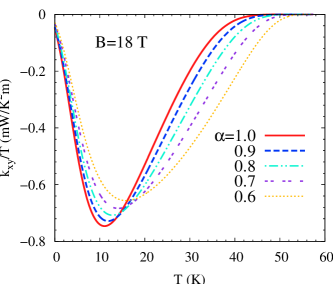
Figure 1: (Color online) Temperature dependence of $k_{xy}/T$ from numerical calculation of Eq. (19) with $\Delta_{0}=\gamma(T^{*}-T)^{\alpha}$. In the calculation, we choose a case in the overdoped regime which is far from the antiferromagnetic phase. $T^{*}=57~{}$K. Other used parameters can be found in the Supplemental Material (see Table SI SM ).

The temperature dependence of the thermal Hall conductivity [$k_{xy}=j_{E}/(t\nabla_{R}T)$ with $t$ being the thickness of the single layer in cuprate superconductors] requires the specific behavior of the ground state (i.e., pairing interaction) to obtain $\Delta_{0}(T)$, and this goes beyond the scope of present analysis. Nevertheless, in Eq. (19), with the increase of $T$ from $0$ to $T^{*}$, $n_{R}$ increases, whereas the order parameter part $\Delta_{0}\partial_{T}\Delta_{0}$, in general, drops slowly at the beginning and then rapidly near $T_{c}$. Thus, a peak behavior in the temperature dependence of $|k_{xy}|$ can be expected. To justify this analysis, we approximately take $\Delta_{0}\sim(T^{*}-T)^{\alpha}$ and perform a numerical calculation of Eq. (19). The numerical results for different $\alpha$ are plotted in Fig. 1. As expected, with the increase of temperature from $T=0~{}$K, $|k_{xy}/T|$ first increases and then decreases, leading to a peak behavior observed around $T=12~{}$K. The experimental finding in the pseudogap phase so far lies in the regime with $T{\geq}14~{}$K and only the decrease of $|k_{xy}/T|$ is observed THCC . In this regime, the experimentally observed linear dependence on magnetic field and temperature dependence as well as negative sign of $k_{xy}/T$ in the pseudogap phase show good agreement with our results. Therefore, we conjecture that the experimentally observed unidentified charge-neutral excitation in the pseudogap phase THCC is the rotating Higgs mode. It is noted that notwithstanding the fact that our computation in Fig. 1 extends to $T=0~{}$K, our result is valid only in the pseudogap regime with $T_{c}<T<T^{*}$.

In conclusion, within the GIKE approach, we have analytically derived the energy spectra of both breathing and rotating Higgs modes of the $d$-wave order parameter for the first time. Then, investigations on their rich dynamic properties have been carried out. Particularly, for the unique rotating Higgs mode in $d$-wave superconductors, it is interesting to find that with longitudinal temperature gradient in pseudogap phase, by magnetic field, this charge-neutral mode generates a thermal Hall current, which is likely to capture recent experimental finding in pseudogap phase of cuprate superconductors THCC .

The authors acknowledge financial support from the National Natural Science Foundation of China under Grants No. 11334014 and No. 61411136001.

References

- (1) P. B. Littlewood and C. M. Varma, Phys. Rev. Lett. 47, 811 (1981); Phys. Rev. B 26, 4883 (1982).
- (2) Y. Nambu, Phys. Rev. 117, 648 (1960).
- (3) V. Ambegaokar and L. P. Kadanoff, Nuovo Cimento 22, 914 (1961).
- (4) J. Goldstone, Nuovo Cimento 19, 154 (1961).
- (5) J. Goldstone, A. Salam, and S. Weinberg, Phys. Rev. 127, 965 (1962).
- (6) J. R. Schrieffer, Theory of Superconductivity (W. A. Benjamin, New York, 1964).
- (7) I. J. R. Aitchison, P. Ao, D. J. Thouless, and X. M. Zhu, Phys. Rev. B 51, 6531 (1995).
- (8) A. F. Volkov and S. M. Kogan, Zh. Eksp. Teor. Fiz 65, 2038 (1974) [Sov. Phys. JETP 38, 1018 (1974)].
- (9) E. A. Yuzbashyan and M. Dzero, Phys. Rev. Lett 96, 230404 (2006).
- (10) V. Gurarie, Phys. Rev. Lett. 103, 075301 (2009).
- (11) N. Tsuji and H. Aoki, Phys. Rev. B 92, 064508 (2015).
- (12) R. Matsunaga and R. Shimano, Phys. Rev. Lett. 109, 187002 (2012).
- (13) R. Matsunaga, Y. I. Hamada, K. Makise, Y. Uzawa, H. Terai, Z. Wang, and R. Shimano, Phys. Rev. Lett. 111, 057002 (2013).
- (14) R. Matsunaga, N. Tsuji, H. Fujita, A. Sugioka, K. Makise, Y. Uzawa, H. Terai, Z. Wang, H. Aoki, and R. Shimano, Science 345, 1145 (2014).
- (15) R. Matsunaga, N. Tsuji, K. Makise, H. Terai, H. Aoki, and R. Shimano, Phys. Rev. B 96, 020505 (2017).
- (16) K. Katsumi, N. Tsuji, Y. I. Hamada, R. Matsunaga, J. Schneeloch, R. D. Zhong, G. D. Gu, H. Aoki, Y. Gallais, and R. Shimano, Phys. Rev. Lett. 120, 117001 (2018).
- (17) H. Chu, M. J. Kim, K. Katsumi, S. Kovalev, R. D. Dawson, L. Schwarz, N. Yoshikawa, G. Kim, D. Putzky, Z. Z. Li, H. Raffy, S. Germanskiy, J. C. Deinert, N. Awari, I. Ilyakov, B. Green, M. Chen, M. Bawatna, G. Christiani, G. Logvenov, Y. Gallais, A. V. Boris, B. Keimer, A. Schnyder, D. Manske, M. Gensch, Z. Wang, R. Shimano, and S. Kaiser, arXiv:1901.06675.
- (18) K. Katsumi, Z. Z. Li, H. Raffy, Y. Gallais, R. Shimano, arXiv:1910.07695.
- (19) Y. Barlas and C. M. Varma, Phys. Rev. B 87, 054503 (2013).
- (20) M. A. Müller, P. A. Volkov, I. Paul, and I. M. Eremin, Phys. Rev. B 100, 140501(R) (2019).
- (21) H. Ding, T. Yokoya, J. C. Campuzano, T. Takahashi, M. Randeria, M. R. Norman, T. Mochiku, K. Kadowaki, and J. Giapintzakis, Nature (London) 382, 51 (1996).
- (22) A. G. Loeser, Z. X. Shen, D. S. Dessau, D. S. Marshall, C. H. Park, P. Fournier, and A. Kapitulnik, Science 273, 325 (1996).
- (23) D. S. Marshall, D. S. Dessau, A. G. Loeser, C. H. Park, A. Y. Matsuura, J. N. Eckstein, I. Bozovic, P. Fournier, A. Kapitulnik, W. E. Spicer, and Z. X. Shen, Phys. Rev. Lett. 76, 4841 (1996).
- (24) M. R. Norman, H. Ding, M. Randeria, J. C. Campuzano, T. Yokoya, T. Takeuchi, T. Takahashi, T. Mochiku, K. Kadowaki, P. Guptasarma, and D. G. Hinks, Nature 392, 157 (1998).
- (25) K. M. Shen, F. Ronning, D. H. Lu, F. Baumberger, N. J. C. Ingle, W. S. Lee, W. Meevasana, Y. Kohsaka, M. Azuma, M. Takano, H. Takagi, and Z. X. Shen, Science 307, 901 (2005).
- (26) J. Wu, A. T. Bollinger, X. He, and I. Božović, Nature 547, 432 (2017).
- (27) F. Yang and M. W. Wu, Phys. Rev. B 98, 094507 (2018).
- (28) F. Yang and M. W. Wu, Phys. Rev. B 100, 104513 (2019).
- (29) The translational symmetry leads to , whereas by time-reversal symmetry.
- (30) See Supplemental Material for additional details of the GIKE and its solution as well as the derivation of the thermal Hall current within path integral method.
- (31) As the practical formation of the -wave order parameter with a certain direction spontaneously breaks the rotational symmetry, according to Goldstone theorem Gm2 there exists a gapless Goldstone boson, which describes the rotational fluctuation of the direction of the -wave order parameter. For the case with order parameter, one finds , and hence, for small fluctuation , , equivalent to the rotational Higgs mode .
- (32) G. Grissonnanche, A. Legros, S. Badoux, E. Lefrancois, V. Zatko, M. Lizaire, F. Laliberté, A. Gourgout, J. S. Zhou, S. Pyon, T. Takayama, H. Takagi, S. Ono, N. D. Leyraud, and L. Taillefer, Nature 571, 376 (2019).
- (33) M. E. Peskin and D. V. Schroeder, An Introduction to Quantum Field Theory (Addison-Wesley, New York, 1995).