Estimating the extent of glioblastoma invasion

Abstract

Glioblastoma Multiforme is a malignant brain tumor with poor prognosis. There have been numerous attempts to model the invasion of tumorous glioma cells via partial differential equations in the form of advection-diffusion-reaction equations. The patient-wise parametrisation of these models, and their validation via experimental data has been found to be difficult, as time sequence measurements are generally missing. Also the clinical interest lies in the actual (invisible) tumor extent for a particular MRI/DTI scan and not in a predictive estimate. Therefore we propose a stationalised approach to estimate the extent of glioblastoma (GBM) invasion at the time of a given MRI/DTI scan. The underlying dynamics can be derived from an instationary GBM model, falling into the wide class of advection-diffusion-reaction equations. The stationalisation is introduced via an analytical solution of the Fisher-KPP equation, the simplest model in the considered model class. We investigate the applicability in 1D and 2D, in the presence of inhomogeneous diffusion coefficients and on a real 3D DTI-dataset.

1 Introduction

Treatment of glioblastoma multiforme (GBM) turmors usually consists of a combination of tumor resection (operation), radio- and chemotherapy (Sathornsumetee et al., 2007). The treatment planning for this type of tumor is particularly challenging, as the medical images do not show a clear boundary and cancerous glia cells infiltrate seemingly healthy tissue far away from the visible center, leading to a diffusive front. Tumor cells have been histologically cultivated from healthy appearing tissue as far as 4 cm away from the bulk of the tumor (Silbergeld and Chicoine, 1997). The non invasive medical imaging modalities may only detect the tumor upwards of a finite density threshold of about $16\%$ (Swanson et al., 2008; Patel and Hathout, 2017), so that tissues are segmented as healty, although they still contain a significant number of tumor cells.

In clinical practice an average extent of this invisible infiltration of 2 cm normal to the visible tumor is assumed. Using mathematical modelling the aim is to estimate the extent of resection and radiotherapy to be applied outside of the tumorous regions visible on the medical images.

Modelling:

Many efforts have been made to mathematically model the behaviour of the tumorous glia cells within the brain. The mathematical approaches are numerous and include a wide range of effects possibly influencing the behaviour of the glioblastoma (GBM) cells. One prominent mathematical approach is to describe the proliferation and the movement of the tumor by macroscopic partial differential equations. Most of these models take the form of diffusion-reaction-advection equations.

Harpold et. al wrote a review article in 2007 about the evolution of mathematical modelling of GBM (Harpold et al., 2007). The modelling started from simple reaction-diffusion equations with exponential growth ($\frac{\partial c}{\partial t}=\nabla(\mathbf{D}\nabla c)+\rho c$) (Tracqui et al., 1995). From here, the extensions from homogeneous diffusion to distinguished diffusivities in grey- and white matter were performed by (Swanson et al., 2000). With the advent of diffusion tensor imaging (DTI) it was also possible to make use of directional information of water diffusion within the brain. Jbabdi et al. (2005) estimated the tumor diffusion from the water diffusion matrices available from DTI and simulated the tumor invasion making full use of the medical imaging information. It was also possible to link the predicted spreading velocity of the Fisher model ($v\approx 2\sqrt{D\rho}$) to experimental data for low-grade gliomas. They effectively found that the increase in radius was linear. Thereby, giving further indication that the tumor growth may be modelled by reaction-diffusion equations (Mandonnet et al., 2003).

This may indicate that the rate of advance can be estimated with the knowledge of the diffusive properties of the surrounding tissue, and the reproductive rate of the tumorous glia cells. There are also quite rigorous approaches to link knowledge on microscopic cell behaviour to macroscopic partial differential equations via upscaling. The mathematical framework was given by (Othmer and Hillen, 2000, 2002; Hillen and Painter, 2013). The underlying idea is to identify the most important influences on the cell’s behaviour on the microscopic and mesoscopic scale and mathematically derive the influence on the macroscopic population dynamic. With this powerful approach it has been possible to microscopically motivate haptotaxis, chemotaxis and proliferation (Engwer et al., 2016, 2015; Hunt and Surulescu, 2017; Jan Kelkel, 2011; Corbin et al., 2018).

Woodward et al. additionally modelled the effect of resection on the tumor invasion, finding some correlation with real survival times of patients (Woodward et al., 1996). A similar approach was taken by Hunt and Surulescu (2017) on more advanced models. They modelled the effect of chemotherapy on the ligand binding rate, the influence of radiation killing cells and the resection itself. The resection was simulated by depleting all tumor cell densities above a threshold (e.g. 20%). They compared different combinations of the simulated treatment. While this approach is more acknowledging to the availability of data, the fundamental problems persist.

Currently, most models strive to describe the full temporal and spatial dynamics of uninterrupted tumor growth but there also have been been approaches to statically estimate the tumor’s invasive profile. Notably Konukoglu et al. formulated travelling-time formulations for the tumor invasion problem in the form of eikonal equations that only rely on the imaging data at the time of diagnosis (Konukolu et al., 2006; Konukoglu et al., 2007). Their results are promising, but the approach does not seem to not have found much traction.

Parameters:

There have been approaches to assess the growth characteristics and parameters in in-vitro experiments, e.g. (Oraiopoulou et al., 2018). It is an open question whether the information gathered in these experiments is transferable to in-vivo situations. Caragher et al. investigated treatments using novel 3D cell culturing methods in the context of GBM therapy developement (Caragher et al., 2019). Even if in-vitro experiments may prove essential in understanding the involved biochemistry and qualitative effects, their use for the validation problem is limited. In order to improve our ability to accurately describe GBM invasion the interlinked problems of parametrisation and availability of data have to be addressed. The reason for this is that the large number of free parameters can not be met with experimental data to estimate them with reasonable accuracy.

Validation:

Although there are a number of mathematical descriptions available, it has proven difficult to derive their parametrisation from medical data or experiments. In medical practice the diagnosis of GBM is often rapidly followed by a combination of tumor resection, radio- and chemotherapy, thereby severely altering the growth characteristics of the tumor (Sathornsumetee et al., 2007). One problem is, that in order to validate any given forward GBM-model given in the form of advection-diffusion-reaction equations, one would need a time-series of DTI/MR/CT scans of the patient, where the tumor growth had been left without cessation. That setup would allow for direct comparison of the in-silico experiments and the medical images of the progressing tumor. One also preferably had these datasets from a large number of representative patients. In order to retrieve a dataset like that, one needed to deprive a high number of patients of live prolonging treatment while undergoing regular medical scans. The ethical impossibility is obvious. It is also questionable whether any such datasets will be available in the near future.

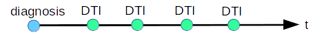
Figure 1: Schematic time line of ideal datasets for the validation of GBM forward models.

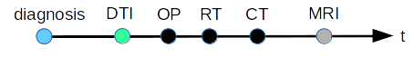
Figure 2: Schematic time line of a realistic sequence of measurements. The initial DTI scan after diagnosis is rapidly followed by a combination of gross tumor resection (OP), radio- and chemotherapy (RT, CT). During treatment, there may be follow-up MRI’s .

Even in more accessible subjects like rodents, it proved difficult to determine a good parametrisation for numerical models. Rutter et al. studied tumor growth in five mice which were injected with tumorous glia cells under controlled conditions. Even with a reportedly careful experimental setup, the resulting tumor sizes varied significantly and fitting parameters of a simple Fisher-KPP tumor model proved difficult (Rutter et al., 2017). Given the goal of improving the ability to accurately describe the tumor invasion in real patients, the problem of validation/falsification has to be addressed.

Contribution:

We present a stationalisation approach, that opens the possibility to estimate the invisible tumor extent at measurement time, building upon existing instationary tumor growth models. It may also alleviate part of the parametrisation problem by only being sensitive to the relative strength of physical effects and not on their absolute quantitative parametrisation. We will first state the class of considered partial differential equations in section 2.1. In section 2.2 we present a methodology to find a stationalised analytical expression for the 1D Fisher-KPP equation, determining the front shape of a travelling wave solution. We also explain how the analytically derived stationalisation term may be used to approximate the tumor density. After numerical verification of the derived gradient distribution, we investigate whether this stationalisation approach is viable in the presence inhomogeneous material properties in section 4. Finally the advantages and shortcomings of the proposed procedure will be critically discussed in 5.

2 Modelling

2.1 Fully anisotropic advection-diffusion-reaction equation

The time-dependent GBM invasion is often modelled by parabolic partial differential equations. We describe the tumor density with the function $u:\Omega\times T\mapsto\mathds{R}$, with the d-dimensional domain $\Omega\subset\mathds{R}^{d}$ and a time range $T=[t_{0},t_{e}]$. The solution $u$ describes the volume percentage of cancerous cells and therefore $0\leq u(\mathbf{x})\leq 1$. The dynamic of the density profile is given in the form of a macroscopic partial differential equation. We consider the time-dependent fully anisotropic advection-diffusion-reaction equation in the following form:

$$\frac{\partial u}{\partial t}-\nabla(\mathbf{D}_{t}(\mathbf{x})\nabla u)-\nabla((\nabla\cdot\mathbf{D}_{t}(x))u) =\rho u(1-u) \Omega\times T,$$ in (1a)

with boundary and initial conditions

$$u(\mathbf{x},0) =g(\mathbf{x}) \Omega,$$ in (1b)

$$\nabla u(\mathbf{x},t) =0 \partial\Omega\times T,$$ on (1c)

with the diffusion parameter $\mathbf{D}_{t}(\mathbf{x})$ being a symmetric positive definite matrix $\mathbf{D}_{t}(\mathbf{x})\in\mathds{R}^{d\times d}$, i.e. the diffusivity can be inhomogeneous and anisotropic. Equation (1) is a prototype model for the invasion of GBM in the sense that many models differ from it merely in the reconstruction of the tumor diffusion matrix $\mathbf{D}_{t}(x)$ from DTI data, or the addition of other chemotaxis terms (Hunt, 2018).

2.2 Stationalisation of the Fisher-KPP equation

In one dimension and for isotropic diffusive properties with ($\mathbf{D}_{t}=1$, $\rho=1$), equation (1) degenerates to the classical Fisher-KPP equation (Kolmogoroff et al., 1988; Fischer, 1937);

$$\frac{\partial u(x^{\prime})}{\partial t}=\Delta u(x^{\prime})+u(x^{\prime})(1-u(x^{\prime})),$$ (2)

with $x^{\prime}\in\mathds{R}$ as a spatial coordinate. The first term may be interpreted as the passive diffusive spread of the cells due to a random walk, the rightmost term as a logistic proliferation term, as often encountered in biological contexts. For the initial conditions:

$$\lim\limits_{x^{\prime}\rightarrow-\infty}{u^{\prime}(x)=1},\leavevmode\nobreak\ \leavevmode\nobreak\ \lim\limits_{x^{\prime}\rightarrow\infty}{u^{\prime}(x)=0},$$

the equation allows travelling wave solutions (Kolmogoroff et al., 1988). These solutions converge over asymptotically long times cales to a wave-front which is constant in shape, moving laterally with a globally constant velocity $v\in\mathds{R}$. With that information, equation (2) can be stated in equivalent form by introducing a co-moving frame $x=x^{\prime}-vt$.

$$0=\Delta u(x)+u(x)(1-u(x))\underbrace{-v\cdot\nabla u(x)}_{\text{ stationalisation}}$$ (3)

The advective term $-v\cdot\nabla u(x)$ results from the coordinate transformation into the comoving frame and can be understood as simply counteracting the lateral movement of the propagating front (Ablowitz and Zeppetella, 1979; Kolmogoroff et al., 1988). We will refer to the advective term and its approximations as the stationalisation term. Any laterally shifted profile $u(x-c)$, with a constant $c\in\mathds{R}$ is equally a solution to (3). The minimum limit speed of the travelling wave solutions has been stated to be

$$v=2\sqrt{D_{t}\rho\leavevmode\nobreak\ }\!,$$

but Kolomogorov also states that there are solutions for speeds higher than $v$. This fact is due to the reaction term acting independently of the local environment. For the limit of diminishing diffusion, the reaction term will induce very high travelling wave speeds for initial conditions which are close to horizontal. Contrarily, the wave speed will be determined to a higher degree by the diffusive flux for initial conditions that fall from 1 to 0 in a very localized region (Kolmogoroff et al., 1988). In the context of glioma invasion only the very rapid spatial decay of tumor density is relevant. Even though the sigmoidal shape of the advancing front profile is formed quite rapidly, it may take asymtotically long to reach a state where the shape of the advancing front is no longer changing. For long time scales and no boundary conditions, a stationary wave form can be given in analytical form for the special wave-speed of $v=\frac{5}{\sqrt{6}}$

$$u(x)=\frac{1}{(1-r\exp(\frac{x}{\sqrt{6}}))^{2}}\leavevmode\nobreak\ ,$$ (4)

where $r=-1$ (Ablowitz and Zeppetella, 1979). We will call that profile the equilibrated wave-form. In the fully equlibrated case, we can state an analytical expression for $\nabla u(x)$. Since the analytical solution is invertible in the relevant range $u\in[0,1]$, we may also express the gradient in terms of $u$. Assuming an analytical expression for $p(u)=v\nabla u(u)$, we may express the comoving 1D Fisher-KKP equation (3) in equivalent form:

$$0=\Delta u+u(1-u)\underbrace{-p(u)}_{\text{ stationalisation}}.$$

The gradient of the analytical solution, can be given as

$$\nabla u=\frac{-\sqrt{\frac{2}{3}}\exp(\frac{x}{\sqrt{6}})}{(1+\exp(\frac{x}{\sqrt{6}}))^{3}}.$$ (5)

The inverse of the analytical solution is given by

$$x(u)=\sqrt{6}\ln\Big{(}\pm\frac{1}{\sqrt{u}}-1\Big{)}.$$ (6)

and represents the mapping from a given amplitude $u$ to the corresponding position $x$ within the wave form profile. Substituting the inverse (6) into the gradient expression(5) yields an analytical term for $\nabla u(u)$ and thereby a closed form for the stationalisation term

$$p(u)=|v|\sqrt{\frac{2}{3}}(1-\sqrt{u})u.$$

Note that the strict equivalence between $p(u)$ and $-v\nabla u$ only holds for the limit case, in which the analytical solution is available. Also, the expression only holds for the case without boundary conditions, i.e. $\Omega\equiv\mathds{R}$. Although this formulation is only strictly equivalent in case of a completely equilibrated wave form, we will use the penalty term $p(u)$ as an approximation of $v\nabla u(u)$ leading to a stationalised wave-pinning type model:

$$0 ={\underbrace{\Delta u+u(1-u)\vphantom{\sqrt{\frac{2}{3}}}}_{\text{tumor model prototype}}}-{\underbrace{|v|\leavevmode\nobreak\ \sqrt{\frac{2}{3}}(1-\sqrt{u})u}_{\text{stationalisation}}} \text{ in }\Omega,$$ (7a)

$$\nabla u(\mathbf{x}) =0 \text{ at }\partial\Omega,$$ (7b)

$$u(\mathbf{x}) =c \text{ at }\partial\Omega_{i}.$$ (7c)

Within the encompassing domain $\Omega$ we define a smaller enclosed domain $\Omega_{i}\subset\Omega$ representing the tumor visible on the medical images. The additional internal boundary condition on $\partial\Omega_{i}$ is used to localize the stationalised solutions.

The Fisher equation is one example out of a family of KPP-type equations which combine a diffusive term with a nonlinear reaction term $f(u)$. The reaction term is often chosen in a manner so that it dynamically connects two fixed points of amplitude: $f(0)=0,f(1)=0,f(0<u<1)>0$. Although an exact analytical description of the stable wave fronts proves difficult, the rough characteristic of propagating fronts found in nature (combustion, bacteria growth etc.) is often similar to a sigmoid function. The gradient distribution of any sigmoid-like travelling wave front will have a similar shape like $p(u)$. For any sigmoidal wave-form $|\nabla u|$ will be zero for $u=0$ and $u=1$ and of higher amplitude for $0<u<1$.

The underlying idea of the stationalisation procedure is, that the gradient distribution, and therefore the penalty term necessary to calculate the travelling wave form stationally, may possibly be approximated to a good degree of accuracy and even for those cases where the analytical solution is not at hand. Considering the general model in the form of (1), we define the corresponding stationalised problem as: Find $u_{s}$ such that

$$0 =\nabla(\mathbf{D}_{t}(\mathbf{x})\nabla u_{s})+\nabla((\nabla\cdot\mathbf{D}_{t}(\mathbf{x}))u_{s})$$

$$\phantom{=}+\rho u_{s}(1-u_{s})-|v|\leavevmode\nobreak\ \sqrt{\frac{2}{3}}(1-\sqrt{u_{s}})u_{s}, \text{ in }\Omega,$$ (8a)

$$\nabla u(\mathbf{x}) =0 \text{ at }\partial\Omega,\leavevmode\nobreak\$$ (8b)

$$u(\mathbf{x}) =c \text{ at }\partial\Omega_{i}.$$ (8c)

The above problem closely resembles the general model (1a) augmented with the penalty term $p(u)$ and internal boundary conditions. The matrix $\mathbf{D_{t}}(\mathbf{x})$ is a reconstruction of the tumor diffusivity from the DTI datasets, $\rho$ is a growth parameter and $v$ the penalty parameter.

It is known that in higher spatial dimensions, the Fisher-KPP equation has related sigmoid-like travelling wave solutions. There are more additional stable wave front patterns in higher dimensions. One of them describes a v-shaped waveform propagating through the two-dimensional medium, which can be interpreted as two straight wave fronts collapsing into each other at a certain angle. Observed in the direction of a bisecting line, this combined wave front is indeed stationary at certain speeds. There also exist spatially oscillating front shapes, but these profiles are only possible for the extension of $u(x)$ out of the relevant range $u\in[0,1]$ (Brazhnik and Tyson, 1999). We focus on cases where the wave propagation occurs as a radial expansion from a centred mass. In the direction of the propagation, equation (4) provides good estimates on the wave fronts profile.

3 Numerical methods and error measures

In this section we discuss the methods used in our numerical experiments to measure the modelling error of the proposed stationalisation. In section 4 we will use the methods to investigate the validity of our approach in a series of problems with growing complexity.

3.1 Numerical scheme

We follow the method of lines approach to split temporal and spatial operators. The temporal discretisation is an implicit-euler scheme, which is unconditinally stable.

For the spatial discretisation we use for simplicity a standard finite element discretisation on cubic grids with multi-linear trial- and test-functions.

The matrix divergences are pre-calculated by a first order finite difference approximation within each grid cell. The inhomogeneous diffusion matrices at the quadrature point are evaluated by nearest neighbour interpolation.

Positivity of our solution might be violated in finite precision calculations. Wherever the numerical iteration leaves the physically sensible range of $u\in[0,1]$, we disregard the reaction term of the given forward- or stationalized model and instead employ the following artificial numerical penalty term

$$n(u)=\begin{cases}-\rho u&\text{if\leavevmode\nobreak\ }u<0\\ \rho(1-u)&\text{if\leavevmode\nobreak\ }u>1.\\ \end{cases}$$ (9)

This is done, because a logistic reaction term $\propto\rho u(1-u)$ may otherwise amplify numerical fluctuations which produce a slightly negative amplitude in $u$.

The stationalisation procedure should be largely independent of the chosen numerical discretisation. The largest source of error does not lie in the numerical treatment, but in the approximations made in the parametrisation and in the estimation of the internal Dirichlet constraints.

3.2 Implementation

The implementation was realized within DUNE software framework (Bastian et al., 2008b, a; Blatt et al., 2016). The finite element discretisation was implemented within dune-pdelab (Bastian et al., 2010). The non-linear system is solved with a classical Newton-Krylov method, using linear search. The linear systems are solved with an AMG- preconditioned BiCGSTAB solver, using the dune-istl module (van der Vorst, 1992; Blatt and Bastian, 2007). The release version for all DUNE modules was 2.6.

For the realistic head model the diffusion matrices were reconstructed by the camino software package (Cook et al., 2006).

3.3 Error measure

In section 4.2 we will investigate the impact of the stationalisation error on the observed tumor front. In this course we will compare the reconstructed tumor front of a fully instationary simulation with the reconstructed tumor front using the stationalisation approach.

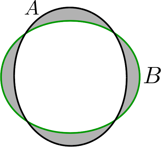
Figure 3: Schematic representation of $A\oplus B$: grey regions

Given a reference solution $u_{a}$, an approximation $u_{b}$ and a threshold value $\theta$ we define two domains $A$ and $B$ as

$$A=\{\mathbf{x}|u_{a}(\mathbf{x})\geq\theta\},\qquad B=\{\mathbf{x}|u_{b}(\mathbf{x})\geq\theta\}.$$

The medically relevant information is the spatial discrepancy between two level-sets ($\partial A,\partial B$) of these density profiles. An absolute measure for this error is the symmetric difference $A\oplus B$, as depicted in Figure 3. It measures those sub-volumes which are either included $A$ but not in $B$, or vice versa. That way, both over- and underestimations of the approximation $u_{b}$ are represented. The most expressive information in the medical context might be the average distance between the two level-sets. We therefore introduce the characteristic level-set distance.

Definition 1 (Characteristic level-set distance)

For a given level-set value $\theta$, we define the characteristic level-set distance between $\partial A$ and $\partial B$ as

$$L_{B}:=\frac{|A\oplus B|}{|\partial A|}.$$ (10)

It quantifies the average distance between the

Assuming a spherical reference geometry for $A$ we can simplify this expression and avoid evaluating $|\partial A|$. Given the radius $r_{A}$ (or an approximate average radius of $A$), $L_{B}$ simplifies to

$$L_{B}^{\text{1d}}=\frac{|A\oplus B|}{2},\quad L_{B}^{\text{2d}}=\frac{|A\oplus B|}{2\pi r_{A}}\quad\text{and}\quad L_{B}^{\text{3d}}=\frac{|A\oplus B|}{4\pi r_{A}^{2}}.$$

3.4 Notes on Uniqueness

The limit solutions to the Fisher equation (2) allow for travelling wave solutions moving in both the positive and negative direction. In the stationalised (co-moving) formulation we find a similar situation. If equation (3) is augmented with a Dirichlet side condition in the form of $u(\mathbf{x_{c}})=c$ within the domain and Neumann boundaries at the border, we may find two solutions mirrored around the constrained point within the profile. Since we want to use an internally constrained region given by segmentation information we may expect two possible solutions to the formulation (3). The first solution corresponds to the stationary approximation to the travelling wave solution of the forward model, which moves outwards from the tumor center, while satisfying the Dirichlet constraint. This solution will have relatively low mass outside the constrained region. The second possible solution corresponds to a travelling wave moving into the constrained region, and will have a high mass on the outside. The two solution types are sketched in Figure 4.

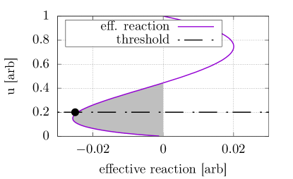
Figure 4: Left: Schematic of high- and low mass solutions (HMS, LMS), both fulfilling the internal Dirichlet constraints (black dots). Right: Plot of effective reaction term consisting of the logistic growth and the penalty term. The penalizing regime is indicated in grey. The visibility threshold is within the penalizing regime.

When considering the effective reaction term consisting of the logistic growth combined with the penalty term, we find that it has a penalizing regime for $0<u<\frac{4}{9}$ and a growth regime for $\frac{4}{9}<u<1$ (Fig. 4). The diffusive process transports mass from high amplitudes to lower amplitudes. The combined reaction term counteracts this process. The visibility threshold, and therefore the constraints, lie within the penalizing regime. In order to select the low mass solution branch, we use initial guesses $u_{s}(x)\ll 1$ which are well within the purely penalizing regime, so that the newton iteration converges to the low mass solution reliably.

4 Numerical results

We present the results of the numerical validation studies of the stationalisation procedure in 1D and 2D. We first compare the gradient distributions of forward simulations with the analytical expression found in equation (2.2) in section 2. After that we compare forward simulations with their stationary approximations and assess the impact of our modelling error on the reconstructed tumor front. We present an easily reproducible 2D example in 4.2.2. Finally we present the applicability to a realistic 3D DTI dataset in 4.3.

4.1 Investigation of modelling error

We will numerically investigate the effect of inhomogeneous diffusion on the gradient distribution, and by this the applicability of the chosen stationalisation term. As the analytic formulation of $\nabla u$ is only valid in the homgeneous 1D case, we expect a modelling error, which we will assess in different test cases.

4.1.1 Artificial imhomogeneous diffusion

We introduce a test cases with randomly perturbed diffusion coefficients.

$$\mathbf{D}_{\beta}=\mathds{1}_{d}\leavevmode\nobreak\ (\delta)^{\frac{1}{d}},$$ (11)

with $\delta$ being a uniformly distributed random value with a spread of $\beta$ around an average of 1. Here, $d$ is the spatial dimension. The exponent of $\delta$ is chosen to allow comparisons between the isotropic homogeneous case and the randomized case, by assuring that the average of the determinants of the diffusive medium are close to 1.0 for every realisation of the random field:

$$|\bar{\mathbf{D}}_{\beta}|=\bar{(\delta)}\approx 1.$$ (12)

We only compare the homogeneous and inhomogeneous case with equal grid resolution. We evaluate the random inhomogeneous diffusion on the dual grid and assume it to be piecewise constant therein. The diffusivity within one dual grid cell is statistically independent from any neighbour. The effect of statistical scattering of the diffusive properties on the macroscopic front speed is non-trivial. Since the global front speed appears as a linear factor in the analytic derivation of the stationalisation term, we may not expect perfect convergence to the analytically derived gradient distribution. The results may however illustrate the effect of realistic datasets.

4.1.2 1D gradient distributions

We consider a one dimensional forward simulation of equation (1) starting from a Gaussian initial condition in the center of a one dimensional domain $x\in[0,200]$. We first simulate the homogeneous case with $D_{t}=1$ where we expect perfect convergence of the gradient distribution to the analytical expression. In the homogeneous case there are no advective terms active, as $\nabla\cdot D_{t}$ is zero. Upon start of the simulation, two travelling waves form and move away from the center of the domain.

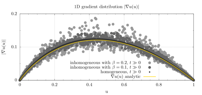
Figure 5: Scatter plot of 1D gradient distribution: magnitude of gradient of 1D wave-front profile. The numerical solution approaches the analytic expression only at asymptotically large time-scales. The underlying characteristic is not destroyed by the introduced inhomogeneities.

After a short initial phase, the wave-fronts in the homogeneous medium asymptotically approach the front shape of the analytical solution (4) and its symmetric counterpart. The front speeds within an inhomogeneous material are slightly perturbed. Similarly the relation $\nabla u(u)$ is disturbed.

In Figure 5 we investigate how the gradient distributions approach the analytical expression for the homogeneous and inhomogeneous case and how strongly it differs from the analytical expression in the case of heterogeous coefficients.

4.1.3 2D gradient distributions

We consider a square domain ($L_{x}=L_{y}=200$) in 2D with a Gaussian initial condition in the center. After the start of the simulation, the wave-front circularly propagates outward from the central point. Slow convergence of the gradient distribution to the analytic expression (2.2) can be replicated in the 2D homogeneous case.

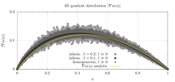
Figure 6: Gradient distribution of a 2D simulation with different spreads in diffusive properties ($\beta=0.0,0.1,0.8$).

Contrary to the one dimensional case, there is an effect of curvature in higher dimensions slowing the convergence towards the 1D gradient distribution. However in the limit case the wave propagation still reduces to a 1D dynamic in the propagation direction (J.D.Murray, 2007). It is obvious that the introduction of random material properties breaks the strict applicability of the stationalisation term. However Figure 6 suggest that also in 2D the underlying polynomial relation between the wave-fronts amplitude and its gradient is merely perturbed by the material properties. Compared to the usual parameter uncertainties, we consider this modelling error small and thus a stationalised solution, making use of the analytical gradient distribution, should still provide reasonable estimates on the density profile. Since the global propagation speed $v$ appears as a linear factor, any process that alters the propagation speed away from the analytical value should have a linear effect on the gradient distribution.

4.2 Effect on estimation of the tumor front

The stationalisation includes a modelling error due to the imperfect approximation of $\nabla u$. The numerical observation in section 4.1 suggests that the average behavior is still well described by our analytic reformulation 7a. In the following we will investigate the impact of this stationalisation error on the actual tumor front. We will use test cases with growing complexity.

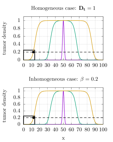
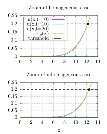
Figure 7: Direct comparison of 1D forward simulations and their stationalizations. The black dots indicate the begin of the internal constraint given by the simulated imaging threshold ($u=0.2$). The domain was discretised into 1000 equidistant elements. Top left.: Initial condition, and states of the forward simulation (homogeneous). Bottom left.: Initial condition, and states of the forward simulation (inhomogeneous). Top right.: Zoom of the forward solution and the corresponding stationalization (homogeneous). Bottom right.: Zoom of the forward solution and the corresponding stationalization (inhomogeneous). Both the forward and the stationalised solution show slight deviations from a smooth decay in the inhomogeneous case. Note that the front speeds are not perfectly identical.

We try to mimic the situation observed in the medical application and present the procedure of estimating the tumor extent at the time of diagnosis. To generate artificial datasets in controlled scenarios, we simulate the carciogenesis by first assuming a small Gaussian initial condition. Secondly, we propagate the density profile for a certain time simulating the uninterrupted tumor growth. Finally, at the time of diagnosis, we use a level-set of $u=0.2$ to represent the thresholded medical imaging modalities. Other choices of threshold value are possible. We then use the thresholded volume as an internal Dirichlet constraint and solve the stationary problem (8a). In this numerical setup both the full forward density profile $u$ and the stationary profile $u_{s}$ are known and compared. In any real world situation only the thresholded image information would be accessible.

4.2.1 1D front reconstruction

We first show results for a simple 1D case with $\mathbf{D}_{t}=1$ and with inhomogeneous coefficients ($\beta=0.2$). By introducing inhomogeneous diffusive coefficients, the advective drift term will produce small contributions to the equation. We chose the penalty parameter $v=\frac{5}{\sqrt{6}}$ and $\rho=1$. The one dimensional setup is not very realistic, but practical to illustrate the procedure. Figure 7 presents a direct comparison of forward simulations with their stationalized counterparts. The snapshots at different times of the forward solution suggest, that the rough form of the advancing front is formed rapidly. If the forward solution converges rapidly towards the form of the analytical solution, with only diminishingly small corrections to the wave fronts shape at larger times, then correspondingly the approximation to the gradient statistic will perform well even early in the simulation. The direct comparisons show that the stationalization produces a reasonable approximation to the full forward solutions. The inhomogeneous coefficients induce small deviations from a smooth front shape, which are present in both the forward simulations profile as well as in the stationalized solution. It is to be expected that wherever the internal constraint results from thresholding of an underlying smooth distribution, the stationalisation will perform well since the real density distribution is close to the equilibrated wave-form.

4.2.2 2D butterfly test case

In order to assess the viability of the stationalisation for more realistic tumor models we now move to two dimensions with inhomogeneous coefficients (eq. (8a)). We set up an inhomogeneous but isotropic field for the diffusion matrix by scaling the unit matrix according to its $x_{1}$ position

$$\mathbf{D}_{t}(\mathbf{x})=\mathds{1}_{2}\leavevmode\nobreak\ (1.0+\sin\Big{(}\frac{3\pi}{L_{x}}x_{1}\Big{)}\leavevmode\nobreak\ 0.9).$$ (13)

This effectively separates the domain in three distinct regions, with the left- and rightmost third of the domain having higher diffusivity and the middle strip having reduced diffusivity. The changes in diffusivity may represent grey and white matter regions in a primitive way. In this example there is more long-range deviation of the diffusive properties than in the 1D examples in section 4.2.1. We again chose the penalty parameter $v=\frac{5}{\sqrt{6}}$ and $\rho=1$. In a medical situation the task is to estimate the region and intensity of radiotherapy to be applied and the area of resection from only the thresholded information visible at the time of diagnosis.

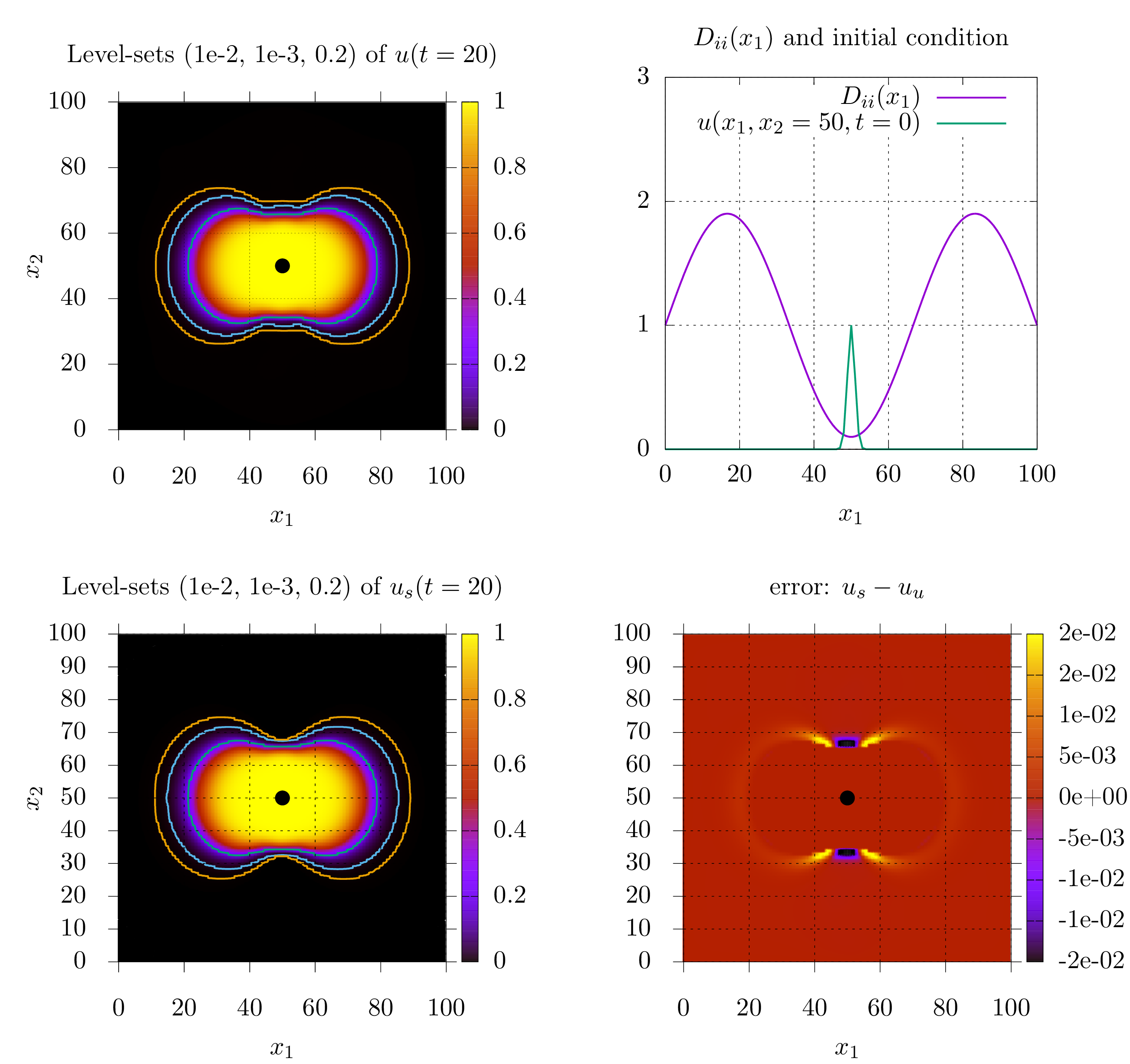
Figure 8: 2D inhomogeneous isotropic testcase. Top left: level-sets on the forward solution at t=20. Top right: diffusivity as given in (13) and horizontal cut through the Gaussian initial condition at $\mathbf{x}=(50,50)$. Bottom left: level-sets on the solution of the stationary problem. Bottom right: Error field indicating regions of over- and underestimation.

Figure 8 compares predictions of the forward simulation of equation (1) with the stationary solutions of equation (8a). The stationalisation greatly benefits from the internally constrained region. Since most of the tumor mass is above the visibility threshold, the stationalization only has to provide the estimation on the surrounding region. Similar to the 1D constrained situation, the stationalisation captures the profile quite well, but slightly overestimates the invasion extent in low density regions.

4.3 3D stationalisation for a realistic dataset

To show the applicability on real patient data, we use the publicly accessible DTI-dataset provided by the camino software project (Cook et al., 2006). We relate the tumor diffusion to the water diffusion by a simple scalar factor:

$$\mathbf{D}_{t}=\alpha\mathbf{D}_{w}.$$ (14)

More advanced reconstructions are possible, but not central to this example. A variety of different tumor diffusion models has been proposed in the literature, see e.g. (Hunt, 2018; Painter and Hillen, 2013; Conte et al., 2020).

parameter	value
$\alpha$	5e-12
$\rho$	1e-6 [1/s]
$v$	2.04e-6 [1/s]

Table 1: Parameters used to scale the terms in (1) and (8a) to realistic ranges. The penalty parameter $v$ has the unit of $1/s$ since we approximated the gradient within the advective term with the analytical expression (2.2).

We use the forward model (1) and the corresponding stationary problem (8a), with the parameters in table 1 to scale the equations to a realistic range. Here $\alpha$ is a dimensionless parameter, $v$ the penalty parameter, and $\rho$ is a growthrate in $1/s$. We again follow the procedure described in section 4.2 and start a forward simulation from a small Gaussian at $t_{0}=0$ until $t_{e}=90d$, and use a level-set ($u=0.2$) as the constrained region for the stationalisation.

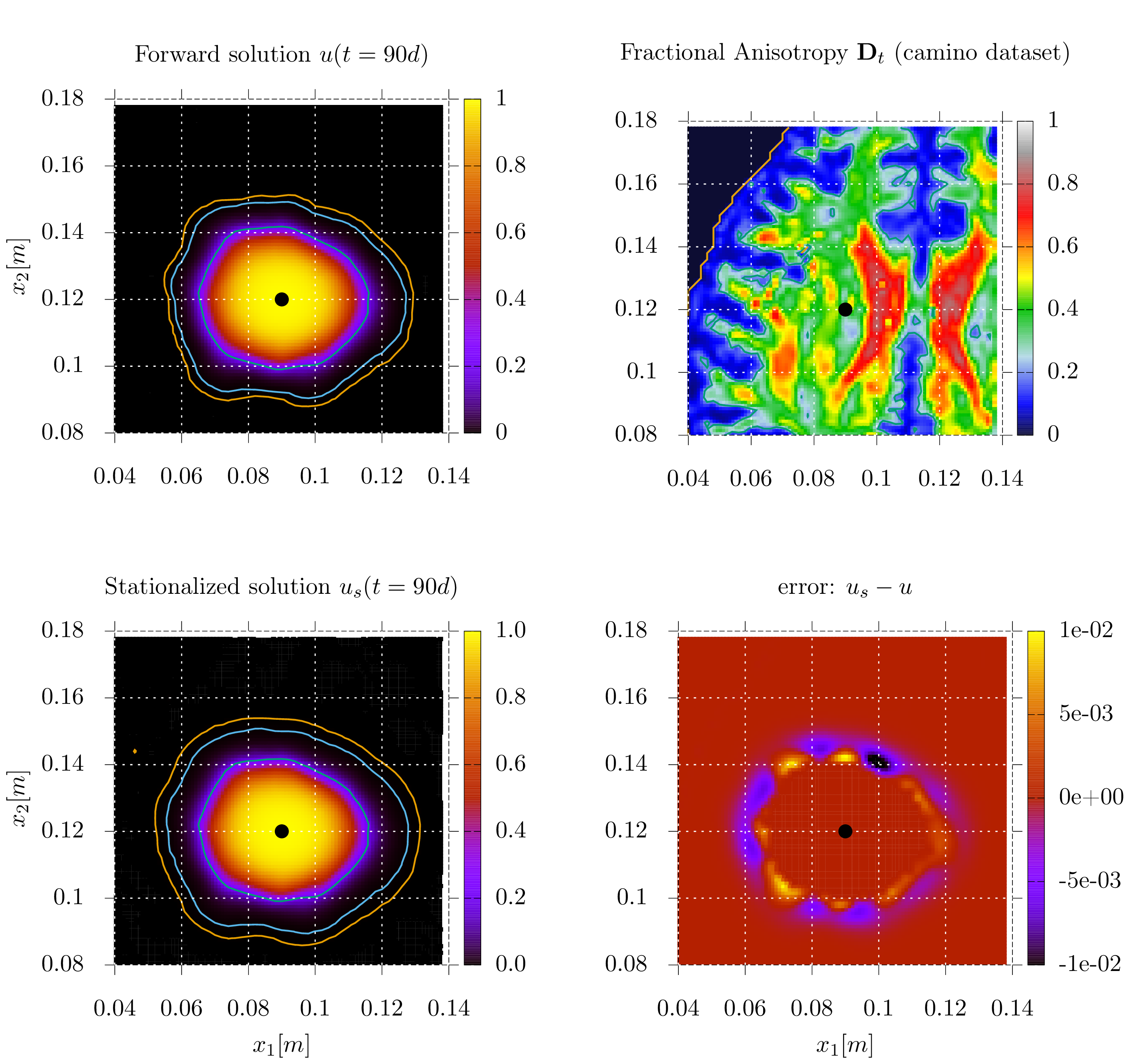
Figure 9: Horizontal slice of the 3D results and dataset. The black dot indicates the position of the small Gaussian initial condition at $x=(0.09m,0.12m,0.05m)$. Top left: level-sets (0.2, 1e-3, 1e-4) on $u(\mathbf{x})$ after 90 days. Top right: Fractional Anisotropy of the reconstructed tumor diffusion matrix $\mathbf{D}_{t}(x)$ from the camino dataset (Cook et al., 2006). Bottom left: Identical level-sets on $u_{s}(\mathbf{x})$. Bottom right: Regions of over- and underestimation by the stationary solution.

Figure 10: Characteristic length errors $L_{B}$ for given level-set values for the 3D example camino dataset. The grey region indicates the errors between the level-sets used in Figure 9.

Figure 9 shows the direct comparison of the forward simulation and the stationalization. All local extentions or reductions induced by the local increase or decrease of the underlying diffusivity are present in both the forward and the stationalized solution. For this particular example, we measured the characteristic levelset distance $L_{B}$ as given in (10) for a series of small levelset values. Figure 10 indicates that the distance error is between $1-3\text{mm}$ for the level-sets chosen in our numerical example. These levelsets were chosen to replicate the current treatment radius of about 2cm.

5 Discussion

We presented a stationalisation approach for the estimation of the glioblastoma invasion extent. The stationalisation approach partially addresses the problems of parametrization and data availability. The stationary simulations do not depend on the complete knowledge of the initial condition to produce reasonable tumor invasion estimates. The thresholded information provided by the medical images might be fully utilized with the limited information it provides. The stationalisation only requires datasets from one point in time, i.e. one DTI scan and a medical segmentation of the tumorous region. This is the data that is routinely gathered in medical practice, as it is used for planning the radiation therapy and resection. Stationary simulations, as presented here, may provide an additional tool in this regard without altering the imaging practices.

The problem of quantifying model parameters is also partly alleviated by the fact that in the stationary formulation the solution depends merely on the strength of the parameters with respect to each other, and not their absolute values. It may be easier to experimentally determine ratio values between the three important parameterized terms: $\mathbf{D}_{t},v$ and $\rho$ than the full set of parameters needed for a forward simulation. Forward models which fit into the form of equation (1) may only produce reliable results if the correct initial condition $g(\mathbf{x})$ is known and the parameters are determined to a reasonable degree of accuracy. In the medical setting the only information at hand is the medical imaging at time of diagnosis. For the forward models to produce reasonable estimates on the tumor invasion profile we would firstly need information on the location and time of the carciogenesis, secondly the information on the non-degraded diffusive properties of the tissue surrounding it and lastly the correct parametrisation on a per-patient basis. We want to emphasise that the temporal dynamics of the tumor growth, although scientifically interesting, are not necessarily relevant in the medical treatment planning. The information needed for treatment with the current techniques is an accurate description of the tumor density field at time of diagnosis.

The derivation of the stationalisation term for the one dimensional Fisher equation is not strictly transferable to tumor models which incorporate medical data or have additional advection terms, but the results from section 4.3 indicate that they may still produce reasonable predictions. If the underlying diffusion matrix field included strong inhomogeneities inducing strong advective terms, the procedure might lose its validity, however an investigation of the given 3D DTI dataset shows that the peclet-number relating the drift and diffusion strength as given in (8a), $\tau=\frac{|v\leavevmode\nobreak\ L|}{|D|}$, stays mostly below 0.3 when $\mathbf{D}_{t}$ is derived from the DTI data by simple scaling (14). Most tumor models show travelling wave characteristics, where the main physical effects include diffusion and nonlinear growth. We recommend close inspection of both the gradient distributions and the peclet numbers if the stationalised model should be extended. The stationalisation procedure should retain its applicability as long as the gradient distribution retains its underlying characteristic, and the distance between medical segmentation and the border induced by the level-sets is not chosen too large. In the case that the presented approximation fails, it may also be possible to introduce more elaborate numerical ways to fit the necessary penalty term locally.

We compared the level-sets of the forward simulation with those of the stationary simulation and found characteristic distances between them of about $L_{B}\approx$ 1.0-3.0mm (Fig. 10). Compared to a fixed-size radius of 2cm around the visible tumor (Chang et al., 2007), these errors seem justifiable. It is of course possible to find an optimal penalty parameter $v$ for a given set of forward model parameters. A medical practitioner might choose the actual level-set value to replicate the current practice of treating a 2 cm radius around the bulk tumor and then use qualitative information in the form of locally recommending an extension or retraction of the treatment radius. The stationary model will correctly capture the effect of the material properties, as presented in Figure 8. Where the tissue is more diffusive, the level-set on $u_{s}$ will overextend the 2 cm radius and where the diffusivity is small, more brain tissue might be left untreated. If the underlying tumor model should be extended, all effects increasing- or diminishing the spread of glia cells will be reflected accordingly in the stationalised solution.

Should time-series datasets become available, then the stationalisation may be used to estimate the initial condition $g(\mathbf{x})$ for a forward simulation from the first dataset. An initial condition calculated in this way should be closer to a presumably smooth real density profile than using a stepped profile with steep gradients.

Naturally the computation of solutions to the stationary problem take less time than a full forward simulation. While compute servers are usually available in academic institutions, the possibility to calculate the results on a regular consumer pc with only short computation times is important in order to transfer such methods into clinical application. The stationary simulation allows for the computation of sets of solutions for varying parameters within a short timeframe. We present exemplary runtimes for the camino dataset on recent hardware for the two cases in Table 2.

simulation type	hardware	runtime
2D, 90 days	Intel i5-7200U ( 4x2.50GHz )	42 sec
2D, stationary	Intel i5-7200U ( 4x2.50GHz )	0.4 sec
3D, 90 days	Intel i5-7200U ( 4x2.50GHz )	1:31h
3D, stationary	Intel i5-7200U ( 4x2.50GHz )	76sec
3D, 90 days	AMD EPYC 7501 (32x 2.0GHz)	18min
3D, stationary	AMD EPYC 7501 (32x 2.0GHz)	9 sec

Table 2: Runtimes for the testcases in two- and three dimensions on different hardware.

5.1 Outlook

There might be further improvements to the stationalisaton approach. Altering the stationalisation term, which currently assumes a globally constant wave-propagation speed, to be sensitive to the local material properties might further improve the results. The proportionality of the wave speed ($v\geq 2\leavevmode\nobreak\ \sqrt{D\rho}$) in the one dimensional Fisher-KPP equation may be an indicator for how a localized penalty parameter could be improved. Instead of choosing a constant $v$ globally, it might be possible to set a penalty factor linearly combined with local information. Thereby incorporating the local increases and decreases in diffusivity into the stationalisation.

In section 4.3 we used a real dataset, but a comparatively primitive tumor model. It should be possible to extend the stationalisation procedure to incorporate additional effects like chemo- or haptotaxis as long as the dynamic of producing travelling wave solutions of sigmoidal shape is not altered by the additions. In the example in section 4.3, we used a level-set on the forward simulation as the internal Dirichlet constraints for the stationalisation. In a medical setting one would directly use the medical segmentation from the DTI/MRI modalities. There are promising advances in generating tumor segmentations in an automated fashion, e.g. BraTumIA (Porz et al., 2014). Automating the process of the segmentation opens up the possibility to use a fully automated process to advise the treatment planning in real patients.

We showed how well a stationalised formulation would perform compared to a forward simulation if all the necessary information were present. The fact that time-series datasets are largely unavailable and therefore no parametrizations can be derived from them, makes direct comparisons between existing tumor models difficult. It is, however possible to compare the stationalized versions of existing models with only the datasets from the time of diagnosis. One could then compare these levelsets to the clinical target volume (CTV) regularly produced in medical practice. This offers an attractive approach to perform a model comparison for a wide range of tumor models proposed in the literature.

References

- Ablowitz and Zeppetella (1979) Ablowitz MJ, Zeppetella A (1979) Explicit solutions of fisher’s equation for a special wave speed. Bulletin of Mathematical Biology 41(6):835–840, DOI 10.1007/BF02462380
- Bastian et al. (2008a) Bastian P, Blatt M, Dedner A, Engwer C, Klöfkorn R, Kornhuber R, Ohlberger M, Sander O (2008a) A Generic Grid Interface for Parallel and Adaptive Scientific Computing. Part II: Implementation and Tests in DUNE. Computing 82(2–3):121–138, DOI 10.1007/s00607-008-0004-9
- Bastian et al. (2008b) Bastian P, Blatt M, Dedner A, Engwer C, Klöfkorn R, Ohlberger M, Sander O (2008b) A Generic Grid Interface for Parallel and Adaptive Scientific Computing. Part I: Abstract Framework. Computing 82(2–3):103–119, DOI 10.1007/s00607-008-0003-x
- Bastian et al. (2010) Bastian P, Heimann F, Marnach S (2010) Generic implementation of finite element methods in the Distributed and Unified Numerics Environment (DUNE). Kybernetika 46:294–315
- Blatt and Bastian (2007) Blatt M, Bastian P (2007) The iterative solver template library. In: Kagström B, Elmroth E, Dongarra J, Wasniewski J (eds) Applied Parallel Computing – State of the Art in Scientific Computing, Springer, Berlin/Heidelberg, pp 666–675
- Blatt et al. (2016) Blatt M, Burchardt A, Dedner A, Engwer C, Fahlke J, Flemisch B, Gersbacher C, Gräser C, Gruber F, Grüninger C, Kempf D, Klöfkorn R, Malkmus T, Müthing S, Nolte M, Piatkowski M, Sander O (2016) The Distributed and Unified Numerics Environment, Version 2.4. Archive of Numerical Software 4(100):13–29, DOI 10.11588/ans.2016.100.26526
- Brazhnik and Tyson (1999) Brazhnik PK, Tyson JJ (1999) On traveling wave solutions of fisher’s equation in two spatial dimensions. SIAM Journal on Applied Mathematics 60(2):371–391
- Caragher et al. (2019) Caragher S, Chalmers AJ, Gomez-Roman N (2019) Glioblastoma’s next top model: Novel culture systems for brain cancer radiotherapy research. Cancers 11(1), DOI 10.3390/cancers11010044
- Chang et al. (2007) Chang EL, Akyurek S, Avalos T, Rebueno N, Spicer C, Garcia J, Famiglietti R, Allen PK, Chao KC, Mahajan A, Woo SY, Maor MH (2007) Evaluation of peritumoral edema in the delineation of radiotherapy clinical target volumes for glioblastoma. International Journal of Radiation Oncology,Biology,Physics 68(1):144 – 150, DOI 10.1016/j.ijrobp.2006.12.009
- Conte et al. (2020) Conte M, Gerardo-Giorda L, Groppi M (2020) Glioma invasion and its interplay with nervous tissue and therapy: A multiscale model. Journal of Theoretical Biology 486:110088, DOI https://doi.org/10.1016/j.jtbi.2019.110088, URL http://www.sciencedirect.com/science/article/pii/S0022519319304576
- Cook et al. (2006) Cook PA, Bai Y, Nedjati-Gilani S, Seunarine KK, Hall MG, Parker GJ, Alexander DC (2006) Camino: Open-source diffusion-mri reconstruction and processing. URL http://www.cs.ucl.ac.uk/research/medic/camino/files/camino_2006_abstract.pdf
- Corbin et al. (2018) Corbin G, Hunt A, Klar A, Schneider F, Surulescu C (2018) Higher-order models for glioa invasion: from a two-scale description to effective equations for mass density and momentum. Math Models Meth Appl Sci
- Engwer et al. (2015) Engwer C, Hillen T, Knappitsch M, Surulescu C (2015) Glioma follow white matter tracts: a multiscale dti-based model. J Math Biol 71:551–582
- Engwer et al. (2016) Engwer C, Hunt A, Surulescu C (2016) Effective equations for anisotropic glioma spread with proliferation: a multiscale approach. J Math Med Biol 33:435–459
- Fischer (1937) Fischer RA (1937) The wave of advance of advantageous genes. Annals of Eugenics 7(4):355–369, DOI 10.1111/j.1469-1809.1937.tb02153.x
- Harpold et al. (2007) Harpold HL, Alvord EC Jr, Swanson KR (2007) The evolution of mathematical modeling of glioma proliferation and invasion. Journal of Neuropathology Experimental Neurology 66(1):1–9, DOI 10.1097/nen.0b013e31802d9000, URL http://dx.doi.org/10.1097/nen.0b013e31802d9000
- Hillen and Painter (2013) Hillen T, Painter KJ (2013) Transport and Anisotropic Diffusion Models for Movement in Oriented Habitats, Springer Berlin Heidelberg, Berlin, Heidelberg, pp 177–222. DOI 10.1007/978-3-642-35497-7˙7, URL https://doi.org/10.1007/978-3-642-35497-7_7
- Hunt (2018) Hunt A (2018) Dti-based multiscale models for glioma invasion. doctoralthesis, Technische Universität Kaiserslautern, URL http://nbn-resolving.de/urn:nbn:de:hbz:386-kluedo-53575
- Hunt and Surulescu (2017) Hunt A, Surulescu C (2017) A multiscale modeling approach to glioma invasion with therapy. Vietnam Journal of Mathematics 45(1):221–240, DOI 10.1007/s10013-016-0223-x, URL https://doi.org/10.1007/s10013-016-0223-x
- Jan Kelkel (2011) Jan Kelkel CS (2011) On some models for cancer cell migration throughtissue networks. Mathematical Biosciences & Engineering 8:575, DOI 10.3934/mbe.2011.8.575, URL http://aimsciences.org//article/id/0fac622a-15b3-4a5d-9a14-4414a389a19f
- Jbabdi et al. (2005) Jbabdi S, Mandonnet E, Duffau H, Capelle L, Swanson KR, Pélégrini‐Issac M, Guillevin R, Benali H (2005) Simulation of anisotropic growth of low‐grade gliomas using diffusion tensor imaging. Magnetic Resonance in Medicine 54(3):616–624, DOI 10.1002/mrm.20625, URL https://doi.org/10.1002/mrm.20625
- J.D.Murray (2007) JDMurray (2007) Mathematical Biology 1: An Introduction. Springer
- Kolmogoroff et al. (1988) Kolmogoroff A, Petrovsky I, Piscounoff N (1988) Study of the diffusion equation with growth of the quantity of matter and its application to a biology problem. In: Pelcé P (ed) Dynamics of Curved Fronts, Academic Press, San Diego, pp 105 – 130, DOI https://doi.org/10.1016/B978-0-08-092523-3.50014-9, URL http://www.sciencedirect.com/science/article/pii/B9780080925233500149
- Konukoglu et al. (2007) Konukoglu E, Sermesant M, Clatz O, Peyrat JM, Delingette H, Ayache N (2007) A recursive anisotropic fast marching approach to reaction diffusion equation: Application to tumor growth modeling. Information Processing in Medical Imaging pp 687–699
- Konukolu et al. (2006) Konukolu E, Clatz O, Bondiau PY, Delingette H, Ayache N (2006) Extrapolating tumor invasion margins for physiologically determined radiotherapy regions. In: Larsen R, Nielsen M, Sporring J (eds) Medical Image Computing and Computer-Assisted Intervention – MICCAI 2006, Springer Berlin Heidelberg, Berlin, Heidelberg, pp 338–346
- Mandonnet et al. (2003) Mandonnet E, Delattre JY, Tanguy ML, Swanson KR, Carpentier AF, Duffau H, Cornu P, Van Effenterre R, Alvord Jr EC, Capelle L (2003) Continuous growth of mean tumor diameter in a subset of grade ii gliomas. Annals of Neurology 53(4):524–528, DOI 10.1002/ana.10528
- Oraiopoulou et al. (2018) Oraiopoulou ME, Tzamali E, Tzedakis G, Liapis E, Zacharakis G, Vakis A, Papamatheakis J, Sakkalis V (2018) Integrating in vitro experiments with in silico approaches for glioblastoma invasion: the role of cell-to-cell adhesion heterogeneity. Scientific reports 8(1):16200–16200, URL https://www.ncbi.nlm.nih.gov/pubmed/30385804
- Othmer and Hillen (2000) Othmer HG, Hillen T (2000) The diffusion limit of transport equations derived from velocity-jump processes read more: https://epubs.siam.org/doi/10.1137/s0036139999358167. SIAM Journal on Applied Mathematics SIAM J. Appl. Math., 61:751–775. (25 pages)
- Othmer and Hillen (2002) Othmer HG, Hillen T (2002) The diffusion limit of transport equations ii: Chemotaxis equations. SIAM Journal on Applied Mathematics 62:1222–1250, DOI https://doi.org/10.1137/S0036139900382772, URL https://doi.org/10.1137/S0036139900382772
- Painter and Hillen (2013) Painter K, Hillen T (2013) Mathematical modelling of glioma growth: The use of diffusion tensor imaging (dti) data to predict the anisotropic pathways of cancer invasion. Journal of Theoretical Biology 323:25 – 39, DOI https://doi.org/10.1016/j.jtbi.2013.01.014, URL http://www.sciencedirect.com/science/article/pii/S0022519313000398
- Patel and Hathout (2017) Patel V, Hathout L (2017) Image-driven modeling of the proliferation and necrosis of glioblastoma multiforme. Theoretical Biology and Medical Modelling 14(1):10, DOI 10.1186/s12976-017-0056-7, URL https://doi.org/10.1186/s12976-017-0056-7
- Porz et al. (2014) Porz N, Bauer S, Pica A, Schucht P, Beck J, Verma RK, Slotboom J, Reyes M, Wiest R (2014) Multi-modal glioblastoma segmentation: Man versus machine. DOI 10.1371/journal.pone.0096873, URL https://doi.org/10.1371/journal.pone.0096873
- Rutter et al. (2017) Rutter EM, Stepien TL, Anderies BJ, Plasencia JD, Woolf EC, Scheck AC, Turner GH, Liu Q, Frakes D, Kodibagkar V, Kuang Y, Preul MC, Kostelich EJ (2017) Mathematical analysis of glioma growth in a murine model. Scientific reports 7(1):2508–2508, URL https://www.ncbi.nlm.nih.gov/pubmed/28566701
- Sathornsumetee et al. (2007) Sathornsumetee S, Reardon DA, Desjardins A, Quinn JA, Vredenburgh JJ, Rich JN (2007) Molecularly targeted therapy for malignant glioma. Cancer 110(1):13–24, DOI 10.1002/cncr.22741
- Silbergeld and Chicoine (1997) Silbergeld DL, Chicoine MR (1997) Isolation and characterization of human malignant glioma cells from histologically normal brain. Journal of Neurosurgery 86(3):525 – 531, URL https://thejns.org/view/journals/j-neurosurg/86/3/article-p525.xml
- Swanson et al. (2000) Swanson KR, Alvord EC, Murray JD (2000) A quantitative model for differential motility of gliomas in grey and white matter. Cell Proliferation 33(5):317–329, DOI 10.1046/j.1365-2184.2000.00177.x
- Swanson et al. (2008) Swanson KR, Rostomily RC, Alvord EC (2008) A mathematical modelling tool for predicting survival of individual patients following resection of glioblastoma: a proof of principle. British Journal of Cancer 98(1):113–119, URL https://doi.org/10.1038/sj.bjc.6604125
- Tracqui et al. (1995) Tracqui P, Cruywagen GC, Woodward DE, Bartoo GT, Murray JD, Alvord Jr EC (1995) A mathematical model of glioma growth: the effect of chemotherapy on spatio-temporal growth. Cell Proliferation 28(1):17–31, DOI 10.1111/j.1365-2184.1995.tb00036.x
- van der Vorst (1992) van der Vorst HA (1992) Bi-cgstab: A fast and smoothly converging variant of bi-cg for the solution of nonsymmetric linear systems. SIAM Journal on Scientific and Statistical Computing 13(2):631–644, DOI 10.1137/0913035, URL https://doi.org/10.1137/0913035, https://doi.org/10.1137/0913035
- Woodward et al. (1996) Woodward DE, Cook J, Tracqui P, Cruywagen GC, Murray JD, Alvord Jr EC (1996) A mathematical model of glioma growth: the effect of extent of surgical resection. Cell Proliferation 29(6):269–288, DOI 10.1111/j.1365-2184.1996.tb01580.x