Abstract

Hamiltonian Monte Carlo (HMC) is a powerful Markov chain Monte Carlo (MCMC) algorithm for estimating expectations with respect to continuous un-normalized probability distributions. MCMC estimators typically have higher variance than classical Monte Carlo with i.i.d. samples due to autocorrelations; most MCMC research tries to reduce these autocorrelations. In this work, we explore a complementary approach to variance reduction based on two classical Monte Carlo “swindles”: first, running an auxiliary coupled chain targeting a tractable approximation to the target distribution, and using the auxiliary samples as control variates; and second, generating anti-correlated ("antithetic") samples by running two chains with flipped randomness. Both ideas have been explored previously in the context of Gibbs samplers and random-walk Metropolis algorithms, but we argue that they are ripe for adaptation to HMC in light of recent coupling results from the HMC theory literature. For many posterior distributions, we find that these swindles generate effective sample sizes orders of magnitude larger than plain HMC, as well as being more efficient than analogous swindles for Metropolis-adjusted Langevin algorithm and random-walk Metropolis.

1 Introduction

Recent theoretical results demonstrate that one can couple two Hamiltonian Monte Carlo (HMC; Neal,, 2011) chains by feeding them the same random numbers; that is, even if the two chains are initialized with different states the two chains’ dynamics will eventually become indistinguishable (Mangoubi and Smith,, 2017; Bou-Rabee et al.,, 2018). These results were proven in service of proofs of convergence and mixing speed for HMC, but have been used by Heng and Jacob, (2019) to derive unbiased estimators from finite-length HMC chains.

Empirically, we observe that two HMC chains targeting slightly different stationary distributions still couple approximately when driven by the same randomness. In this paper, we propose methods that exploit this approximate-coupling phenomenon to reduce the variance of HMC-based estimators. These methods are based on two classical Monte Carlo variance-reduction techniques (sometimes called “swindles”): antithetic sampling and control variates.

In the antithetic scheme, we induce anti-correlation between two chains by driving the second chain with momentum variables that are negated versions of the momenta from the first chain. When the chains anti-couple strongly, averaging them yields estimators with very low variance. This scheme is similar in spirit to the antithetic-Gibbs sampling scheme of Frigessi et al., (2000), but is applicable to problems where Gibbs may mix slowly or be impractical due to intractable complete-conditional distributions.

In the control-variate scheme, following Pinto and Neal, (2001) we run an auxiliary chain targeting a tractable approximation to the true target distribution (i.e., a distribution for which computing or estimating expectations is cheap), and couple this auxiliary chain to the original HMC chain. The auxiliary chain can be plugged into a standard control-variate swindle, which yields low-variance estimators to the extent that the two chains are strongly correlated.

These two schemes can be combined to yield further variance reductions, and are especially effective when combined with powerful preconditioning methods such as transport-map MCMC (Parno and Marzouk,, 2014) and NeuTra (Hoffman et al.,, 2019), which not only reduce autocorrelation time but also increase coupling speed. When we can approximate the target distribution well, our swindles can reduce variance by an order of magnitude or more, yielding super-efficient estimators with effective sample sizes significantly larger than the number of steps taken by the underlying Markov chains.

2 Hamiltonian Monte Carlo Swindles

2.1 Antithetic Variates

Suppose $X$ is a random variable following some distribution $P(x)$ and we wish to estimate $\mathbb{E}_{P}[f(X)]$. If we have two (not necessarily independent) random variables $X_{1},X_{2}$ with marginal distribution $P$ then

$$\mathop{\textrm{Var}}\left[\frac{f(X_{1})+f(X_{2})}{2}\right]= \frac{1}{4}\big{(}\mathop{\textrm{Var}}[f(X_{1})]+\mathop{\textrm{Var}}[f(X_{2})]$$

$$+2\mathop{\textrm{Cov}}[f(X_{1}),f(X_{2})]\big{)}$$

When $f(X_{1})$ and $f(X_{2})$ are negatively correlated the average of these two random variables will have a lower variance than the average of two independent draws from the distribution of $X$. We will exploit this identity to reduce the variance of the HMC algorithm.

First we consider the usual HMC algorithm to generate samples from the probability distribution with density function $P(x)\triangleq\mathcal{Z}^{-1}\exp(-U(x))$ on $\mathbb{R}^{D}$ (Neal,, 2011). The quantity $\mathcal{Z}$ is a possibly unknown normalization constant. Let $\mathcal{N}(0,I_{D})$ be the standard multivariate normal distribution on $\mathbb{R}^{d}$ with mean $0$ and covariance $I_{D}$ (the identity matrix in $D$ dimensions). For position and momentum vectors $q$ and $p$ each in $\mathbb{R}^{D}$ define the Hamiltonian $H(q,p)=\frac{1}{2}||p||^{2}+U(q)$. Also suppose that $\Psi_{H,T}(q,p)$ is a symplectic integrator (Hairer et al.,, 2006) that numerically simulates the physical system described by the Hamiltonian $H$ for time $T$, returning $q^{\prime},p^{\prime}$. A popular such method is the leapfrog integrator. The standard Metropolis-adjusted HMC algorithm is:

1:procedure HMC($X_{0},n,T$)

2:  for $i=0$ to $n-1$ do

3:   $\triangleright$ Sample momentum from normal distribution

4:   Sample $p_{i}\sim\mathcal{N}(0,I_{D})$.

5:   $\triangleright$ Symplectic integration

6:   Set $(q_{i+1},p_{i+1})=\Psi_{H,T}(X_{i},p_{i})$.

7:   Sample $b_{i}\sim\mathrm{Unif}([0,1])$.

8:   Set $X_{i+1}$ = MHAdj($X_{i}$, $q_{i+1}$, $p_{i}$, $p_{i+1}$, $b_{i}$, $H$)

9:  end for

10:end procedure

11:procedure MHAdj($q_{0}$, $q_{1}$, $p_{0}$, $p_{1}$, $b$, $H$)

12:  if $b<\min(1,\exp(H(q_{0},p_{0})-H(q_{1},p_{1})))$ then

13:   return $q_{1}$.

14:  else

15:   return $q_{0}$.

16:  end if

17:end procedure

The output is a sequence of samples $X_{1},\ldots,X_{n}$ that converges to $P(x)$ for large $n$ (Neal,, 2011).

Next, we consider a pair of coupled HMC chains:

1:procedure HMC-COUPLED($X_{0},Y_{0},n,T$)

2:  for $i=0$ to $n-1$ do

3:   Sample $p_{i}\sim\mathcal{N}(0,I_{D})$.

4:   Set $p^{\prime}_{i}=p_{i}$. $\triangleright$ Shared $p_{i}$

5:   Set $(q_{i+1},p_{i+1})=\Psi_{H,T}(X_{i},p_{i})$.

6:   Set $(q^{\prime}_{i+1},p^{\prime}_{i+1})=\Psi_{H,T}(Y_{i},p^{\prime}_{i})$.

7:   Sample $b_{i}\sim\mathrm{Unif}([0,1])$. $\triangleright$ Shared $b_{i}$

8:   Set $X_{i+1}$ = MHAdj($X_{i}$, $q_{i+1}$, $p_{i}$, $p_{i+1}$, $b_{i}$, $H$)

9:   Set $Y_{i+1}$ = MHAdj($Y_{i}$, $q^{\prime}_{i+1}$, $p^{\prime}_{i}$, $p^{\prime}_{i+1}$, $b_{i}$, $H$)

10:  end for

11:end procedure

Considering either the $X_{i}$’s or $Y_{i}$’s in isolation, this procedure is identical to the basic HMC algorithm, so if $X_{0}$ and $Y_{0}$ are drawn from the same initial distribution then marginally the distributions of $X_{1:n}$ and $Y_{1:n}$ are the same. However, the chains are not independent, since they share the random $p_{i}$’s and $b_{i}$’s. In fact, under certain reasonable conditions on $U$ it can be shown that the dynamics of the $X_{i}$ and the $Y_{i}$ approach each other. More precisely, under these conditions each step in the Markov Chain is contractive in the sense that

$$\mathbb{E}[||X_{n+1}-Y_{n+1}||]<c\mathbb{E}[||X_{n}-Y_{n}||]$$

for some constant $c<1$ depending on $U$ and $T$.

Now suppose that $U$ is symmetric about some (possibly unknown) vector $\mu$, so that we have $U(x)=U(2\mu-x)$, and we replace line 4 with

Set $p^{\prime}_{i}=-p_{i}$

We call the new algorithm HMC-ANTITHETIC. With HMC-ANTITHETIC, the sequence $(X_{1},2\mu-Y_{1}),(X_{2},2\mu-Y_{2}),\ldots$ is a coupled pair of HMC chains for the distribution given by $U(x)$. After all, it is the same as the original coupled algorithm apart from $Y_{i},q^{\prime}_{i}$ and $p_{i}^{\prime}$ being reflected. So both $X_{i}$ and $Y_{i}$ converge to the correct marginal distribution $\mathcal{Z}^{-1}\exp(-U(x))$. More interestingly, if $X$ and $2\mu-Y$ couple we now have that

$$\mathbb{E}[||X_{n+1}+Y_{n+1}-2\mu||]<c\mathbb{E}[||X_{n}+Y_{n}-2\mu||].$$

This implies that for large enough $n$

$$\begin{split}X_{n}+Y_{n}&=2\mu+O(c^{n})\\ X_{n}-\mu&=-(Y_{n}-\mu)+O(c^{n}),\end{split}$$ (1)

so we expect the $X_{i}$ and $Y_{i}$ to become perfectly anti-correlated exponentially fast. This means that we can expect $\frac{1}{2n}\sum_{i}f(X_{i})+f(Y_{i})$ to provide very good estimators for $\mathbb{E}[f(X)]$, at least if $f$ is monotonic (Craiu and Meng,, 2005).

For many target distributions of interest, $U(x)=U(2\mu-x)$ holds only approximately. Empirically, approximate symmetry generates approximate anti-coupling, which is nonetheless often sufficient to provide very good variance reduction (see section 4).

2.2 Control Variates

The method of control variates is another classic variance-reduction technique (Botev and Ridder,, 2017). Define

$$\begin{split}Z=f(X)-\beta^{\top}(g(Y)-\mathbb{E}[g(Y)]).\end{split}$$ (2)

By linearity of expectation, $\mathbb{E}[Z]=\mathbb{E}[f(X)]$ for any $\beta$ and $g$, so $Z$ is an unbiased estimator of $\mathbb{E}[f(X)]$. But, if $f(X)$ and $g(Y)$ are correlated and $\beta$ is chosen appropriately, the variance of $Z$ may be much lower than that of $f(X)$. In particular,

$$\begin{split}\mathop{\textrm{Var}}(Z)&=\mathbb{E}[(f(X)-\mathbb{E}[f(X)]-\beta^{\top}(g(Y)-\mathbb{E}[g(Y)]))^{2}]\end{split}$$ (3)

That is, the variance of $Z$ is the mean squared error between $f(X)-\mathbb{E}[f(X)]$ and the predictor $\beta^{\top}(g(Y)-\mathbb{E}[g(Y)])$. An estimate of the optimal $\beta$ can thus be obtained by linear regression. If this predictor is accurate, then the variance of $Z$ may be much lower than that of $f(X)$.

In the absence of an analytic value for $\mathbb{E}[g(Y)]$ we use multilevel Monte Carlo as described in (Botev and Ridder,, 2017), plugging in an unbiased estimator $\hat{g}$ of $\mathbb{E}[g(Y)]$. If the variance of $\hat{g}$ can be averaged away more cheaply than that of $f(X)$, then this multilevel Monte Carlo scheme can still confer a very significant computational benefit.

We can modify HMC-COUPLED to yield a control-variate estimator by replacing line 5 with the line

Set $(q^{\prime}_{i+1},p^{\prime}_{i+1})=\Psi_{H^{\prime},T}(Y_{i},p^{\prime}_{i})$.

and line 9 with the line

Set $Y_{i+1}$= MHAdj($Y_{i}$, $q^{\prime}_{i+1}$, $p^{\prime}_{i}$, $p^{\prime}_{i+1}$, $b_{i}$, $H^{\prime}$)

where $H^{\prime}$ is a different Hamiltonian that approximates $H$:

$$\begin{split}H^{\prime}(q,p)\triangleq\frac{1}{2}||p||^{2}-\log Q(q)\end{split}$$ (4)

for a density $Q$ chosen so that $Q\approx P$ and so that $\mathbb{E}_{Q}[Y]$ is tractable to compute or cheap to estimate. Finally, we define the variance-reduced chain

$$\begin{split}Z_{i,j}=f_{j}(X_{i})-\beta_{j}^{\top}(f(Y_{i})-\hat{\mathbb{E}}_{Q}[f(Y)]),\end{split}$$ (5)

where $f$ is a vector-valued function whose expectation we are interested in, and $\hat{\mathbb{E}}_{Q}[f(Y)]$ is an unbiased estimator of $\mathbb{E}_{Q}[f(Y)]$. We call this new algorithm HMC-CONTROL.

In English, the idea is to drive a pair of HMC chains with the same randomness but with different stationary distributions $P$ and $Q$ and use the chain targeting $Q$ as a control variate for the chain targeting $P$. The more closely $Q$ approximates $P$, the more strongly the two chains will couple, the more predictable $X$ will be given $Y$, and the lower the variance of $Z$ will become.

2.3 Combining Antithetic and Control Variates

HMC-ANTITHETIC and HMC-CONTROL rely on different coupling strategies, so in principle we can get further variance reduction by combining the two algorithms. Specifically, we can augment the $X$ and $Y$ chains in HMC-CONTROL with antithetic chains $X^{-}$ and $Y^{-}$, and combine $X^{-}$ and $Y^{-}$ to get an antithetic variance-reduced chain $Z^{-}$ as in Equation 5. If we choose the approximating distribution $Q$ to be symmetric about a known mean $\mu$ (for example, if $Q$ is a multivariate Gaussian) then a further optimization is to directly set $Y_{i}^{-}=2\mu-Y_{i}$. We denote the resultant algorithm HMC-CVA, and provide a listing of it in Appendix A. Figure 1 shows that HMC-CVA does induce the variance-reduced chains $Z^{+}$ and $Z^{-}$ to anti-couple, leading to a further variance reduction.

2.4 Preconditioning $U$

HMC-CVA works best when $P$ is approximately symmetric, and can be approximated by a tractable symmetric distribution $Q$ with known mean. Clearly not all target distributions satisfy this condition. Following Parno and Marzouk, (2014); Hoffman et al., (2019), we can partially resolve this issue by applying a change of variables $\tilde{x}\triangleq m^{-1}(x)$ to $P$ such that $P(\tilde{x})=P(x)|\frac{\partial m}{\partial\tilde{x}}|\approx\mathcal{N}(\tilde{x};0,I)\triangleq Q(\tilde{x})$, and running our samplers in $\tilde{x}$ space instead of $x$ space. This also increases HMC’s mixing speed.

The method is agnostic to how we obtain the transport map $m$; in our experiments we use variational inference with reparameterization gradients (e.g.; Kucukelbir et al.,, 2017) to minimize the Kullback-Leibler (KL) divergence from $Q(x)$ to $P(x)$ (or equivalently from $\mathcal{N}(0,I)$ to $P(\tilde{x})$).

3 Related Work

3.1 Markov Chain coupling

Coupling has long been used as a theoretical tool to study and prove convergence behavior of Markov chains and therefore Markov Chain Monte Carlo (MCMC) algorithms (Lindvall,, 1992). For example Bou-Rabee et al., (2018) use coupling to show that the steps in the HMC algorithm are contractive. Coupling has also been used to derive practical algorithms. Glynn and Rhee, (2014), Jacob et al., (2017), and Heng and Jacob, (2019) use Markov chain coupling to give unbiased estimators.

3.2 Markov Chain Monte Carlo and Antithetic Variates

In early work in this area, Hastings, (1970) uses an alternating sign-flip method, similar to antithetic variates, to reduce the variance of samples from generated with a single Markov Chain targeting a symmetric toy distribution. Green and Han, (1992) further develop of this method, still using a single Markov chain.

Frigessi et al., (2000) propose an antithetic Gibbs sampling scheme very similar in spirit to antithetic HMC, in which each one-dimensional complete conditional distribution is sampled by CDF inversion driven by antithetic uniform noise. Antithetic HMC has three main advantages over antithetic Gibbs: first, HMC often mixes much more quickly than Gibbs sampling (so there is less variance to eliminate in the first place); second, HMC can be applied to models with intractable complete-conditional distributions (Frigessi et al., (2000) found that switching to a Metropolis-within-Gibbs scheme to handle intractable complete conditionals reduced the variance-reduction factor to 2, which is no better than what could be obtained by running an independent chain); finally, HMC is more amenable than Gibbs to preconditioning schemes (Parno and Marzouk,, 2014; Hoffman et al.,, 2019), which accelerate both mixing and coupling.

3.3 Coupling and Control Variates

In previous work the method of control variates has been proposed as a method to reduce variance in MCMC methods. However, control variates require the use of an approximating distribution whose properties can be computed either analytically, or much more efficiently than the target distribution. Dellaportas and Kontoyiannis, (2012) note that finding such distributions has posed a significant challenge. That paper provides a general purpose method for a single Markov chain that can be used whenever we have an explicit computation of $\mathbb{E}[g(X_{n+1})|X_{n}=x]$ for a Markov chain $\{X_{i}\}$ and for certain linear functions $g$. Andradóttir et al., (1993) use a smoothing method to improve the efficiency of Monte Carlo simulations, and use approximations to smoothing to derive control variates. Baker et al., (2019) use control variates to reduce the variance arising from stochastic gradients in Langevin dynamics.

Goodman and Lin, (2009) use a coupled pair of Markov chains, both of which have marginal distributions equal to the target distribution. The second of these chains is then used to provide proposals for a Metropolis-Hastings algorithm that generates samples from an approximation to the target distribution. It is this approximate distribution which serves as their control variate.

Our control-variate HMC scheme can be seen as an adaptation of the method of Pinto and Neal, (2001), who only considered coupling schemes based on Gibbs sampling and random-walk Metropolis, neither of which typically mixes quickly in high dimensions (Neal,, 2011). The Gibbs scheme was reported to couple effectively, but is limited to problems with tractable complete conditionals, while the random-walk Metropolis scheme required a small step size (which dramatically slows mixing) to suppress the rejection rate and ensure strong coupling (an issue we will see in section 4). By contrast, HMC is applicable to any continuously differentiable target distribution, and its rejection rate can be kept low without sacrificing mixing speed.

4 Experiments

We test the proposed variance reduction schemes on three posterior distributions.

4.1 Target Distributions

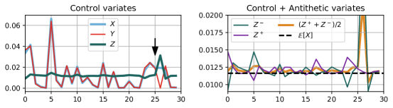
Figure 1: On the left, a trace of 30 steps of the HMC chain $X_{i}$ with its coupled chain $Y_{i}$. Both chains are estimating the posterior variance of a single dimension for the logistic regression posterior. By using $Y_{i}$ as a control variate to $X_{i}$, we obtain a variance-reduced chain $Z$. The coupling is strong, and is only interrupted when the two chains make opposite decisions in the Metropolis-Hastings correction (arrow). On the right, we can average $Z$ (labeled $Z^{+}$ for emphasis) and its antithetically coupled chain $Z^{-}$ to further reduce the variance of the estimator.

Logistic regression:

We first consider a simple Bayesian logistic regression task, with the model defined as follows:

$$\begin{split}w_{d}&\sim\mathcal{N}(0,1);\quad y_{n}\sim\mathrm{Bern}(\sigma(x_{n}^{\top}w))\end{split}$$ (6)

where $w$ are the covariate weights, $\mathrm{Bern}$ is the Bernoulli distribution and $\sigma$ is the sigmoid function. We precondition the sampler using a full-rank affine transformation.

We apply the model to the German credit dataset (Dua and Graff,, 2019). This dataset has 1000 datapoints and 24 covariates (we add a constant covariate for the bias term, bringing the total to 25) and a binary label. We standardize the features to have zero mean and unit variance.

Sparse logistic regression:

To illustrate how variance reduction works with non-linear preconditioners and complicated posteriors we consider a hierarchical logistic regression model with a sparse prior:

$$\begin{split}\tau&\sim\mathrm{Gam}(\alpha=0.5,\beta=0.5)\\ \lambda_{d}&\sim\mathrm{Gam}(\alpha=0.5,\beta=0.5)\\ w_{d}&\sim\mathcal{N}(0,1);\quad y_{n}\sim\mathrm{Bern}(\sigma(x_{n}^{\top}(\tau w\circ\lambda)))\end{split}$$ (7)

where $\mathrm{Gam}$ is the Gamma distribution, $\tau$ is the overall scale, $\lambda$ are the per-component scales, $w$ are the non-centered covariate weights, and $w\circ\lambda$ denotes the elementwise product of $w$ and $\lambda$. The sparse gamma prior on $\tau$ and $\lambda$ imposes a soft-sparsity prior on the overall weights. This parameterization uses D=51 dimensions. Following Hoffman et al., (2019), we precondition the sampler using a neural-transport (NeuTra) stack of 3 inverse autoregressive flows (IAFs) (Kingma et al.,, 2016) with 2 hidden layers per flow, each with 51 units, and the ELU nonlinearity (Clevert et al.,, 2015).

Item Response Theory

As a high-dimensional test, we consider the 1PL item-response theory model.

$$\begin{split}\delta\sim\mathcal{N}(0.75,&1);\quad\alpha_{i}\sim\mathcal{N}(0,1);\quad\beta_{j}\sim\mathcal{N}(0,1)\\ y_{ij}&\sim\mathrm{Bern}(\sigma(\alpha_{i}-\beta_{j}+\delta))\,|i,j\in\mathcal{T}\end{split}$$ (8)

where $\delta$ is the mean student ability, $\alpha_{i}$ is ability of student $i$, $\beta_{j}$ is the difficulty of question $j$, $y_{ij}$ is whether a question $j$ was answered correctly by student $i$ and $\mathcal{T}$ is the set of student-question pairs in the dataset. We precondition the sampler using a full-rank affine transformation.

We apply the model to the benchmark dataset from the Stan example repository which has 400 students, 100 unique questions and a total of 30105 questions answered. In total, the posterior distribution of this model has D=501 dimensions.

4.2 Sampling procedure

As described in Section 2.4, we train a transport map $m$ by variational inference with reparameterization gradients to minimize $\mathrm{KL}(Q||P)$, where $Q(x)=\mathcal{N}(m^{-1}(x);0,I)|\frac{\partial m^{-1}}{\partial x}|$ (Kucukelbir et al.,, 2017). The resultant distribution is used as the initial state for the HMC sampler. To compute accurate estimates of performance, we run a few thousands of chains for 1000 steps, discarding the first 500 to let the chains reach their stationary distribution.

We tune the hyper-parameters of the HMC sampler to maximize the effective sample size (ESS) normalized by the number of gradient evaluations of $U$, while making sure the chain remains stationary. ESS is a measure of the variance of MCMC estimators, defined as $ESS=N\mathop{\textrm{Var}}[\hat{\mathbb{E}}_{MC}[f(X)]]/\mathop{\textrm{Var}}[\hat{\mathbb{E}}_{MCMC}[f(X)]]$.

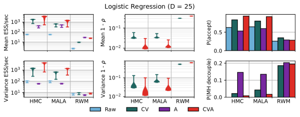
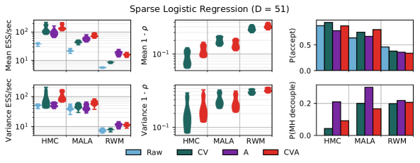
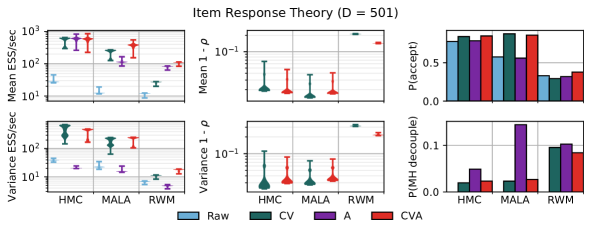
Figure 2: Performance of the various variance reductions schemes when estimating the posterior mean and variance for the two target distributions. First column shows violin plots (aggregated across the dimensions of $X$) of ESS/sec (log scale), each algorithm tuned as described in the main text. Second column shows the correlation achieved at the optimal set of hyperparameters (log scale). Top panel of third column shows the acceptance probabilities of the MCMC chains, while the bottom panel shows the probability of two chains decoupling due to the Metropolis-Hastings adjustment step. For all quantities, we compute the mean across 10 independent runs.

We measure chain stationarity using the potential scale reduction metric (Gelman and Rubin,, 1992). The ESS is estimated using the autocorrelation method with the Geyer initial monotone sequence criterion to determine maximum lag (Geyer,, 2011; Vehtari et al.,, 2019).

We estimate and use $\beta$ for all the chains. This introduces some bias in the estimator, although the estimator remains consistent (Pinto and Neal,, 2001). All experiments were run on a Tesla P100 GPU. The source code is available at https://github.com/google-research/google-research/tree/master/hmc_swindles.

4.3 Results

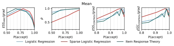
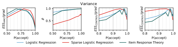
Figure 3: Effect on ESS/grad and $\rho$ when varying the number of leapfrog steps while keeping HMC trajectory length constant for different functions (rows) and probability distributions (different lines). For raw HMC, the optimal ESS/grad is obtained by choosing an acceptance probability in the 0.6-0.9 regime (first column). For HMC-CONTROL decreasing the step size raises $\rho$ (second column) and ESS/grad (third column), up to a point where the original chain efficiency drops below what variance reduction can compensate for, at an acceptance probability near 0.95. As a tuning heuristic, we can predict the location of the optimal acceptance rate by leaning on the theoretical bounds on ESS/grad and empirical $\rho$ estimate (final column).

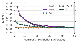
Figure 4: Median held-out test negative log-likelihood for logistic regression, lower is better. The x-axis measures the number of averaged models, including the cost of evaluating any antithetic samples, control variates, and expectations under $Q$ (assuming the latter is available in closed form). The MAP estimate of the parameters provides a variance-free estimate, but it is suboptimal compared to a fully Bayesian model average. Without variance reduction, the raw HMC estimator requires averaging many independent samples to reach parity with the MAP estimator. The HMC-CONTROL and HMC-CVA estimators make accurate predictions with very few function evaluations; HMC-ANTITHETIC is less efficient, but still much faster than independent samples.

For simple $P$’s like the logistic-regression posterior distribution, we observe that $X$ and its control variate $Y$ couple very well leading to dramatic variance reduction in the $Z$ chain (Figure 1, left panel). The two chains only decouple when the Metropolis-Hastings decision is different between the two chains. Note that, since the uniform $b_{i}$’s are shared, not every rejection leads to decoupling.

Adding an antithetic control-variate chain $Z^{-}$ further reduces the variance of the estimator (Figure 1, right panel). As hoped, the antithetic variance-reduced chains $Z^{-}$ are clearly anti-correlated.

Moving beyond qualitative results, we examine ESS/sec values for various algorithms and test problems, evaluated on estimators of the means and variances of the posteriors. For each distribution, we run 10 independent evaluation runs, average across the runs and then report the ESS/sec for each dimension, summarized by a violin plot (Figure 2, first column). We normalize ESS by wall-clock running time to control for running additional chains (or taking different numbers of leapfrog steps for HMC). Running antithetic chains is more expensive than the control-variate chains, as the latter use a cheaper-to-evaluate Hamiltonian (e.g. a Gaussian vs the full model joint distribution) We compare our proposed schemes to the analogous schemes described in earlier work (Frigessi et al.,, 2000; Pinto and Neal,, 2001), applied to Metropolis-adjusted Langevin algorithm (MALA)(Roberts and Rosenthal,, 1998) and Random-Walk Metropolis (RWM) (Metropolis et al.,, 1953).

Overall, the variance reduction schemes improve upon the non variance-reduced algorithms, with the control variates combined with antithetic variates typically outperforming the two techniques individually. Our HMC-based and MALA schemes outperform RWM by over an order of magnitude. This can in part be explained by the high correlations attainable by HMC and MALA (Figure 2, second column), in part because unlike RWM, they can be efficient at high acceptance rates (Figure 2, third column, top panel). A big source of de-correlation are the Metropolis-Hastings adjustment disagreements, which happen much less frequently for HMC and MALA than in RWM (Figure 2, third column, top panel). HMC-based schemes tend to be a few times more efficient than MALA.

A weakness of the antithetic schemes is that they provide less benefit when the the estimated function is symmetric about the mean. In particular, $(\sigma(x^{\top}w)-\mathbb{E}_{P}[\sigma(x^{\top}w)])^{2}$ is close to being an even function in $w-\mathbb{E}_{P}[w]$. This causes the antithetic schemes to be worse than regular MCMC when estimating the variance for the logistic regression and item response theory posteriors, but in case of the asymmetric distribution for sparse logistic regression this is less pronounced. Despite this, in most cases combining control variates and antithetic variates yields some efficiency gains even when estimating variance.

The sparse logistic regression is a significantly more difficult problem, and correspondingly we do not see as much benefit from the variance-reduction techniques. Even with the powerful IAF approximating distribution, the correlation between the coupled chains is not very high, but we still get a several-fold reduction in variance.

The ESS of the variance reduced chain can be related to the ESS of the original chain as

$$ESS_{CONTROL} =ESS_{HMC}/(1-\rho^{2})$$ (9)

$$ESS_{ANTITHETIC} =2ESS_{HMC}/(1+\rho),$$ (10)

for HMC-CONTROL and HMC-ANTITHETIC respectively, where $\rho$ is the correlation coefficient between the corresponding pairs of chains. This suggests that efficiency can be improved by increasing the correlation between the paired chains. This can be done by reducing the step size, but doing so also reduces the efficiency of the original chain. In practice there is exists some optimal step size smaller than is optimal for a single HMC chain, but larger than would maximize the correlation, the exact numerical value of which depends on the details of $f(\cdot)$ and the approximating distributions. We examine this tradeoff empirically by finding an optimal trajectory length (same as in Figure 2), and then varying the number of leapfrog steps and step size to hold trajectory length constant. This study confirms the basic intuition above (Figure 3, first three columns). In practice, we recommend targeting an acceptance rate in the vicinity of 0.95 for distributions similar to ones examined here.

When explicit tuning is desired, we propose a heuristic based on replacing the $ESS_{orig}$ in Equation 9 with an upper bound on the ESS from (Beskos et al.,, 2010):

$$ESS_{HMC}/grad\leq CP(accept)(\Phi(1-P(accept)/2))^{0.5},$$ (11)

where $C$ depends on the distribution, $f(\cdot)$ and the HMC trajectory length and then doing a number of pilot runs to estimate $\rho$. Unlike ESS, $\rho$ can be readily estimated using comparatively few samples, and when plugged into Equation 9 together with Equation 11 yields a quantity $\widehat{ESS}_{CONTROL}/grad$ captures the maximum efficiency as a function of acceptance probability (Figure 3, last column).

A practical application of the variance-reduction schemes is to reduce the cost of accurate predictions on new data. While Bayesian model averaging can provide good accuracy, if it is implemented via MC sampling each test-time example may have to be evaluated many times to reduce the variance of the ensemble prediction. With HMC swindles, we expect this to be less of a problem. To test this use case, we split the German credit dataset randomly into train and test sets using a 90%/10% split, and then compared the test set negative log-likelihood between the various estimators (Figure 4). Raw HMC requires averaging many predictions to reach an acceptable level of variance, while CV-HMC immediately produces accurate predictions.

5 Discussion

We have presented two variance reduction schemes for HMC based on approximate coupling. Despite the added computation, combining both schemes results in improved effective sample size rates. An alternate way of interpreting this result is that when running multiple chains in parallel, converting some of those chains to control variates and antithetic variates is a more efficient way of using a fixed compute budget.

Our experiments have not supported broad effectiveness of the antithetic scheme when used in isolation, in part because it relies on the hard-to-control symmery of the target density. Despite this, it is very easy to implement and there seems little reason not to use it. The control variate scheme is generally applicable, but relies on the practicitioner being able to construct efficient and accurate approximate distributions. This is an impediment to broad use, but as more work is done to make this process automatic through the use of powerful invertible neural networks we hope this becomes less of an issue in the future. Overall, these techniques promise to yield estimates of posterior expectations with extremely low bias and variance, bringing the dream of near-exact posterior inference closer to reality.

Appendix A HMC-CVA Algorithm

We denote the original chain $X$ and its corresponding control variate $Y$ as $X^{+}$ and $Y^{+}$ for emphasis.

1:procedure HMC-CVA($X^{+}_{0},X^{-}_{0},Y^{+}_{0},n,T$)

2:  for $i=0$ to $n-1$ do

3:   Sample $p^{+}_{i}\sim\mathcal{N}(0,I_{D})$.

4:   Set $p^{-}_{i}=-p^{+}_{i}$.

5:   Set $p^{\prime}_{i}=p^{+}_{i}$. $\triangleright$ Shared $p_{i}$

6:   Set $(q^{+}_{i+1},p^{+}_{i+1})=\Psi_{H,T}(X^{+}_{i},p^{+}_{i})$.

7:   Set $(q^{-}_{i+1},p^{-}_{i+1})=\Psi_{H,T}(X^{-}_{i},p^{-}_{i})$.

8:   Set $(q^{\prime}_{i+1},p^{\prime}_{i+1})=\Psi_{H^{\prime},T}(Y^{+}_{i},p^{\prime}_{i})$.

9:   Sample $b_{i}\sim\mathrm{Unif}([0,1])$. $\triangleright$ Shared $b_{i}$

10:   Set $X^{+}_{i+1}$ = MHAdj($X^{+}_{i}$, $q^{+}_{i+1}$, $p^{+}_{i}$, $p^{+}_{i+1}$, $b_{i}$, $H$).

11:   Set $X^{-}_{i+1}$ = MHAdj($X^{-}_{i}$, $q^{-}_{i+1}$, $p^{-}_{i}$, $p^{-}_{i+1}$, $b_{i}$, $H$).

12:   Set $Y^{+}_{i+1}$ = MHAdj($Y^{+}_{i}$, $q^{\prime}_{i+1}$, $p^{\prime}_{i}$, $p^{\prime}_{i+1}$, $b_{i}$, $H^{\prime}$).

13:   Set $Y^{-}_{i+1}=2\mu-Y^{+}_{i+1}$.

14:  end for

15:  Compute unbiased estimate $\hat{\mathbb{E}}_{Q}[f(Y)]$.

16:  Estimate optimal $\beta$ by linear regression.

17:  for $i=1$ to $n$ do

18:   Set $Z^{+}_{i,j}=f_{j}(X^{+}_{i})-\beta_{j}^{\top}(f(Y^{+}_{i})-\hat{\mathbb{E}}_{Q}[f(Y)])$.

19:   Set $Z^{-}_{i,j}=f_{j}(X^{-}_{i})-\beta_{j}^{\top}(f(Y^{-}_{i})-\hat{\mathbb{E}}_{Q}[f(Y)])$.

20:   Set $Z_{i}=\frac{1}{2}(Z^{+}_{i}+Z^{-}_{i})$.

21:  end for

22:end procedure

References

- Andradóttir et al., (1993) Andradóttir, S., Heyman, D. P., and Ott, T. J. (1993). Variance reduction through smoothing and control variates for markov chain simulations. ACM Transactions on Modeling and Computer Simulation (TOMACS), 3(3):167–189.
- Baker et al., (2019) Baker, J., Fearnhead, P., Fox, E. B., and Nemeth, C. (2019). Control variates for stochastic gradient MCMC. Statistics and Computing, 29(3):599–615.
- Beskos et al., (2010) Beskos, A., Pillai, N. S., Roberts, G. O., Sanz-Serna, J. M., and Stuart, A. M. (2010). Optimal tuning of the Hybrid Monte-Carlo Algorithm.
- Botev and Ridder, (2017) Botev, Z. and Ridder, A. (2017). Variance Reduction, pages 1–6. American Cancer Society.
- Bou-Rabee et al., (2018) Bou-Rabee, N., Eberle, A., and Zimmer, R. (2018). Coupling and Convergence for Hamiltonian Monte Carlo. ArXiv e-prints.
- Clevert et al., (2015) Clevert, D.-A., Unterthiner, T., and Hochreiter, S. (2015). Fast and accurate deep network learning by exponential linear units (elus). In International Conference on Learning Representations.
- Craiu and Meng, (2005) Craiu, R. V. and Meng, X.-L. (2005). Multiprocess parallel antithetic coupling for backward and forward Markov Chain Monte Carlo. ArXiv Mathematics e-prints.
- Dellaportas and Kontoyiannis, (2012) Dellaportas, P. and Kontoyiannis, I. (2012). Control variates for estimation based on reversible markov chain monte carlo samplers. Journal of the Royal Statistical Society: Series B (Statistical Methodology), 74(1):133–161.
- Dua and Graff, (2019) Dua, D. and Graff, C. (2019). UCI machine learning repository.
- Frigessi et al., (2000) Frigessi, A., Gåsemyr, J., and Rue, H. (2000). Antithetic coupling of two Gibbs sampler chains. The Annals of Statistics, 28(4):1128–1149.
- Gelman and Rubin, (1992) Gelman, A. and Rubin, D. B. (1992). Inference from iterative simulation using multiple sequences. Statistical Science.
- Geyer, (2011) Geyer, C. J. (2011). Introduction to Markov Chain Monte Carlo. CRC press.
- Glynn and Rhee, (2014) Glynn, P. W. and Rhee, C.-H. (2014). Exact estimation for markov chain equilibrium expectations. J. Appl. Probab., 51A:377–389.
- Goodman and Lin, (2009) Goodman, J. B. and Lin, K. K. (2009). Coupling control variates for markov chain monte carlo. J. Comput. Physics, 228(19):7127–7136.
- Green and Han, (1992) Green, P. J. and Han, X.-l. (1992). Metropolis methods, gaussian proposals and antithetic variables. In Stochastic Models, Statistical methods, and Algorithms in Image Analysis, pages 142–164. Springer.
- Hairer et al., (2006) Hairer, E., Lubich, C., and Wanner, G. (2006). Geometric Numerical Integration: Structure-Preserving Algorithms for Ordinary Differential Equations; 2nd ed. Springer, Dordrecht.
- Hastings, (1970) Hastings, W. K. (1970). Monte carlo sampling methods using markov chains and their applications.
- Heng and Jacob, (2019) Heng, J. and Jacob, P. E. (2019). Unbiased hamiltonian monte carlo with couplings. Biometrika, 106(2):287–302.
- Hoffman et al., (2019) Hoffman, M., Sountsov, P., Dillon, J. V., Langmore, I., Tran, D., and Vasudevan, S. (2019). Neutra-lizing bad geometry in hamiltonian monte carlo using neural transport. arXiv preprint arXiv:1903.03704.
- Jacob et al., (2017) Jacob, P. E., O’Leary, J., and Atchadé, Y. F. (2017). Unbiased Markov chain Monte Carlo with couplings. arXiv e-prints, page arXiv:1708.03625.
- Kingma et al., (2016) Kingma, D. P., Salimans, T., and Welling, M. (2016). Improving variational inference with inverse autoregressive flow. Advances in Neural Information Processing Systems, (2011):1–8.
- Kucukelbir et al., (2017) Kucukelbir, A., Tran, D., Ranganath, R., Gelman, A., and Blei, D. M. (2017). Automatic differentiation variational inference. Journal of Machine Learning Research.
- Lindvall, (1992) Lindvall, T. (1992). Lectures on the Coupling Method. Wiley Series in Probability and Statistics - Applied Probability and Statistics Section. Wiley.
- Mangoubi and Smith, (2017) Mangoubi, O. and Smith, A. (2017). Rapid Mixing of Hamiltonian Monte Carlo on Strongly Log-Concave Distributions. ArXiv e-prints.
- Metropolis et al., (1953) Metropolis, N., Rosenbluth, A. W., Rosenbluth, M. N., Teller, A. H., and Teller, E. (1953). Equation of state calculations by fast computing machines. The journal of chemical physics, 21(6):1087–1092.
- Neal, (2011) Neal, R. M. (2011). MCMC using Hamiltonian dynamics. In Handbook of Markov Chain Monte Carlo. CRC Press New York, NY.
- Parno and Marzouk, (2014) Parno, M. and Marzouk, Y. (2014). Transport map accelerated markov chain monte carlo. arXiv preprint arXiv:1412.5492.
- Pinto and Neal, (2001) Pinto, R. L. and Neal, R. M. (2001). Improving Markov chain Monte Carlo Estimators by Coupling to an Approximating Chain.
- Roberts and Rosenthal, (1998) Roberts, G. O. and Rosenthal, J. S. (1998). Optimal scaling of discrete approximations to langevin diffusions. Journal of the Royal Statistical Society: Series B (Statistical Methodology), 60(1):255–268.
- Vehtari et al., (2019) Vehtari, A., Gelman, A., Simpson, D., Carpenter, B., and Bürkner, P.-C. (2019). Rank-normalization, folding, and localization: An improved R for assessing convergence of MCMC.