Quantum simulation of Unruh-DeWitt detectors with nonlinear optics

Abstract

We propose a method for simulating an Unruh-DeWitt detector, coupled to a 1+1-dimensional massless scalar field, with a suitably-engineered $\chi^{(2)}$ nonlinear interaction. In this simulation, the parameter playing the role of the detector acceleration is played by the relative inverse-group-velocity gradient inside the nonlinear material. We identify experimental parameters that tune the detector energy gap, acceleration, and switching function. This system can simulate time-dependent acceleration, time-dependent detector energy gaps, and non-vacuum initial detector-field states. Furthermore, for very short materials, the system can simulate the weak anti-Unruh effect, in which the response of the detector decreases with acceleration. While some Unruh-related phenomena have been investigated in nonlinear optics, this is the first proposal for simulating an Unruh-DeWitt detector in these systems.

The Unruh-DeWitt (UDW) detector model unruh1976notes ; dewitt1979general ; unruh1984happens predicts that an accelerating observer in vacuum will see blackbody radiation where an inertial observer would see none—this is known as the Unruh effect earman2011unruh . Due to the prohibitively large accelerations required, however, the effect is yet to be verified experimentally. Nevertheless, one can simulate the physics of this effect by engineering a Hamiltonian of the same form in a different, more controllable, system. Experimental realization of a quantum simulation of the Unruh effect could generate new insight and stimulate ideas across different fields of physics.

The Unruh effect is closely connected to the phenomenon of two-mode squeezing walls2007quantum , well-known in quantum nonlinear optics (NLO). This makes NLO a natural candidate for simulating the effect, and indeed some related phenomena have already been studied—specifically, simulations of black-hole horizons philbin2008fiber and the Unruh-Davies effect guedes2019spectra . Several other systems have also been investigated for simulating physics related to the Unruh effect fedichev2003gibbons ; fedichev2004observer ; paraoanu2014recent ; rodriguez2017synthetic ; hu2019quantum , but NLO holds particular promise due to our ability to fabricate and control such systems. New aspects of Unruh-effect-related phenomena are still being discovered, e.g. carballo2019unruh , and their simulation in NLO could produce new insights.

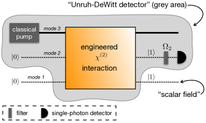
Figure 1: Schematic representing three modes interacting via an engineered $\chi^{(2)}$ interaction (input on the left and output on the right). Modes 1 and 2 are initially prepared in the vacuum state $\ket{0}$, while mode 3 contains a classical pump field. During interaction, a pair of photons is created (one photon in mode 1 and the other in mode 2). An analogy is made between the $\chi^{(2)}$ interaction (Eq. (5)) and a UDW detector coupled to a massless scalar field (Eq. (1)): mode 1 maps to the scalar field while mode 2 (along with other elements in the shaded grey region) maps to the UDW detector. The shaded grey area encloses the elements that determine the UDW detector energy gap, i.e., the frequency of the pump field, the properties of the nonlinear material, and the filter frequency $\Omega_{2}$, as described in Table 1. Detection of a photon in mode 2 corresponds to UDW detection.

In this paper, we consider a quantum simulation of the Unruh effect formulated in terms of UDW detectors. Concretely, we make the analogy between the interaction of two quantum modes of a downconversion process (FIG. 1) and the interaction of a non-inertial detector—i.e. a UDW detector—with a scalar field. This is in contrast to what has been done before where the downconverted state was the analogue for the TMSV of the Rindler wedges alsing2004teleportation . We compute the first-order transition probability amplitudes for both processes and compare them. In doing so, we draw an analogy between the relative inverse-group-velocity gradient inside the nonlinear material and the acceleration of the UDW detector.

Our proposal explicitly identifies which experimental parameters play the role analogous to the detector energy gap, acceleration, and switching function. The downconversion can simulate time-dependent acceleration, time-dependent detector energy gaps olson2011entanglement , and non-vacuum initial detector-field states aspachs2010optimal . Furthermore, we show that for very short crystals, one can also simulate the anti-Unruh effect brenna2016anti , specifically, the weak anti-Unruh effect garay2016thermalization in which the response of the detector decreases with acceleration. garay2016thermalization

I The Unruh-DeWitt detector

An Unruh-DeWitt detector couples to a 1+1-dimensional scalar, massless Klein-Gordon field $\phi(x(\tau),t(\tau))$ through the Hamiltonian garay2016thermalization ; scully1997 :

$$H(\tau)={} \lambda\eta(\tau)m(\tau)\phi(x(\tau),t(\tau))\,,$$ (1)

where $\lambda$ is a small coupling constant with dimension length^-1, $\eta(\tau)$ is a dimensionless switching function, and $m(\tau)$ is the detector’s monopole operator (dimensionless). Here, and in the rest of this paper, we work with natural units $\hbar=c=1$. The time evolution of $m(\tau)$, where $\tau$ is the proper time in the frame of the detector, is assumed to be $m(\tau)=e^{iH_{0}\tau}m(0)e^{-iH_{0}\tau}$, where $H_{0}$ is the free Hamiltonian of the detector. The coordinates $t$ and $x$ describe the Minkowski coordinates associated to an inertial frame.

The scalar field $\phi(x(\tau),t(\tau))$ can be expanded in plane-wave solutions of the Klein-Gordon equation. For massless fields propagating in a single direction it is conventional to work with frequency $\omega_{k}$ rather than wavenumber labels. We thus expand the field (in the interaction picture) in terms of plane waves:

$$\phi(x(\tau),t(\tau))=\int\frac{d\omega_{k}}{\sqrt{4\pi\omega_{k}}}(a(\omega_{k})e^{-i\omega_{k}q(\tau)}+\mathrm{h.c.})\,,$$ (2)

where $q(\tau)=t(\tau)-x(\tau)$ and $[a(\omega_{k}),a^{\dagger}(\omega_{k^{\prime}})]=\delta(\omega_{k}-\omega_{k^{\prime}})$. As evident from Eq. (2), the scalar field is dimensionless (in natural units), as expected for a field defined on 1+1 spacetime milonni2013quantum .

Our goal is to show that the UDW Hamiltonian in Eq. (1) can be simulated with a quantum NLO Hamiltonian. Modifying the quantum NLO Hamiltonian directly to account for the analogue of detector acceleration poses significant technical challenges. In this paper, we thus consider a more manageable approach, and show the equivalence between the two systems by comparing the transition amplitudes at first order. We leave demonstrating the equivalence between the Hamiltonians for future work.

We start the detector in the ground state $\ket{g}$, and take the field to be in the Minkowski vacuum state $\ket{0}$. For a detector turned on at time $\tau_{i}$ and off at time $\tau_{f}$, the conditional probability amplitude (to first order), $\mathcal{A}$, of finding the detector in the excited state $\ket{e}$ given the field is in the single-particle state $\ket{\omega}=a^{\dagger}(\omega)\ket{0}$, is

$$\mathcal{A}={} -i\bra{\omega}\bra{e}\int_{\tau_{i}}^{\tau_{f}}\mathrm{d}\tau H(\tau)\ket{0}\ket{g}\,.$$ (3)

In Appendix A, we show that this can be rewritten as

$$\mathcal{A}={} b(\omega)\int_{\tau_{i}}^{\tau_{f}}\mathrm{d}\tau\eta(\tau)e^{i\Omega\tau}e^{i\omega q(\tau)}\,,$$ (4)

with $b(\omega)=-i\lambda/\sqrt{4\pi\omega}\bra{e}m(0)\ket{g}$ and where $\Omega=E_{e}-E_{g}$ is the energy gap of the detector. The transition amplitude is not typically written this way, so to relate the expression in Eq. (4) to known results, we briefly discuss a few special cases.

For an inertial detector, $t(\tau)=\gamma\tau$ and $x(\tau)=x_{0}+vt=x_{0}+v\gamma\tau$ where $\gamma=(1-v^{2})^{-1/2}$ and $\tau_{f}=-\tau_{i}=T$, and thus $\mathcal{A}=e^{ikx_{0}}\mathrm{sinc}((\Omega+\gamma(\omega-kv))T)/T\sqrt{\pi\omega}$, as found in sriramkumar1996finite . In the limit $T\rightarrow\infty$, one gets $\mathcal{A}\sim\delta(\Omega+\gamma(\omega-kv))$. Since $kv\leq|k||v|<\omega$ and $\Omega>0$, the argument of the delta function is always positive and the detection is forbidden on the grounds of energy conservation. For a uniformly accelerating observer, $x(\tau)=a^{-1}\cosh(a\tau)$ and $t(\tau)=a^{-1}\sinh(a\tau)$, giving $q(\tau)=-a^{-1}e^{-a\tau}$. The limit $T\rightarrow\infty$, yields the famous result that an observer, accelerating through a vacuum, sees a thermal field. Concretely, in this limit, $|\mathcal{A}|^{2}=(e^{2\pi\Omega/a}-1)^{-1}/2a\Omega\omega$, which has a Planckian form in $\Omega$ with a temperature $\beta^{-1}=a/2\pi$ sriramkumar1996finite .

II The analogy with SPDC

In a $\chi^{(2)}$ nonlinear-optical process, a nonlinear material mediates the interaction between three photons. An example of this is SPDC, in which high-energy pump photons are converted into pairs of lower energy photons. $\chi^{(2)}$ processes have widespread application in quantum computation Kok2007 , quantum communication Gisin2007 as sources of non-classical light and quantum interactions donohue2015theory , and quantum metrology Higgins2007 ; Nagata2007 , as well as in more specialized areas such as quantum imaging Brida2010 , quantum lithography Boto2000 , or optical coherence tomography Nasr2008 . Here, we consider a new application as an analogue of the UDW detector.

The interaction Hamiltonian for a three-wave mixing process in a waveguide is yang2008spontaneous :

$$\begin{split}H_{\textsc{s}}(t)={}&-\frac{1}{3\epsilon_{0}}\int d\mathbf{r}\Gamma_{ijk}^{(2)}(\mathbf{r})\hat{D}^{i}(\mathbf{r},t)\hat{D}^{j}(\mathbf{r},t)\hat{D}^{k}(\mathbf{r},t)\,,\end{split}$$ (5)

where $\Gamma^{(2)}(\mathbf{r})$ is a tensor related to the more commonly-used nonlinear tensor $\chi^{(2)}(\mathbf{r})$ via Eq. (15) in yang2008spontaneous , and $\hat{D}$ are the quantized displacement field operators.

Let us assume that we have three fields present in the process (labelled by $1,2,3$), which all have zero overlap with each other, either due to non-overlapping frequencies or orthogonal polarization. Let us also assume that one of the fields ($3$) is intense, non-depleting, and can be treated classically. Under this assumption, both Eqs. (1) and (5) describe the interaction between two quantum systems: Eq. (1) describes the interaction between a UDW detector and a quantized scalar massless field while Eq. (5) describes the interaction between one quantized EM field and a second quantized EM field.

We now identify the massless scalar field with the field in mode 1, and the UDW detector with the field in mode 2. With this analogy, we start modes 1 and 2 in the vacuum state and interact them, with the classical pump field centred at $\Omega_{3}$, in the nonlinear material. After the interaction, we send mode 2 (the UDW detector) through a spectral filter at $\Omega_{2}$ to fix the UDW detector’s energy gap. Subsequent detection of the photon in mode 2 corresponds to UDW detection. This process is shown schematically in FIG. 1.

UDW parameters	SPDC parameters	Correspondence
Detector trajectory $q(\tau)=t(\tau){-}x(\tau)$	Relative inverse GV $\Delta v_{g}(z)^{-1}$	$q(\tau)\leftrightarrow\int_{v\tau_{i}}^{v\tau}\Delta v_{g}(\zeta)^{-1}d\zeta$
Switching function $\eta(\tau)$	Nonlinear susceptibility $\chi^{(2)}(z)$	$\eta(\tau)\leftrightarrow\frac{\chi^{(2)}(v\tau)v}{\sqrt{n_{1}(\Omega_{3}-\Omega_{2};v\tau)n_{2}(\Omega_{2};v\tau)n_{3}(\Omega_{3};v\tau)}}$
	Refractive index $n_{j}(\omega,z)$
Detector energy gap $\Omega(\tau)$	Phase mismatch $\Delta k_{0}(z)$	$\Omega(\tau)\leftrightarrow(\Delta k_{0}(v\tau){-}\Delta v_{g}(v\tau)^{-1}(\Omega_{3}{-}\Omega_{2}))v$
	Relative inverse GV $\Delta v_{g}(z)^{-1}$
Scaling coefficient $b(\omega)$	Spectral pump amplitude $\alpha(\omega)$	$b(\omega)\leftrightarrow i\kappa\alpha(\Omega_{2}+\omega)$
	Coupling strength $\kappa$
Interaction time $\Delta\tau=\tau_{f}-\tau_{i}$	Waveguide length $L=z_{f}-z_{i}$	$v\Delta\tau\leftrightarrow L$

Table 1: Summary of UDW parameters and the corresponding SPDC parameters. The detector trajectory $q(\tau)$ determines the acceleration. The phase mismatch $\Delta k_{0}(z)$ and relative inverse group velocity (GV) $\Delta v_{g}(z)^{-1}$ are defined below Eqs. (8). The coupling strength $\kappa$ is defined in Appendix B. The scaling velocity $v$ is defined above Eq. (9). $\Omega_{3}$ is the mean pump frequency and $\Omega_{2}$ is the frequency of the filter in mode 2.

To compute the corresponding amplitude, we make some further simplifying assumptions. Let us assume that the fields propagate collinearly along $z$ through a waveguide with only one transverse mode that is uniform over a cross-sectional area. Under the assumptions that the tensor nature of $\chi^{(2)}(\mathbf{r})$ and the vector nature of the mode profiles of the displacement field can be neglected, $\chi^{(2)}(z)$ can be taken to characterize the strength of the nonlinearity along the waveguide. We also consider that the refractive index can vary along the length of the waveguide.

For a waveguide starting at position $z_{i}$ and ending at position $z_{f}$, the probability amplitude (to first order), $\mathcal{A}_{\textsc{s}}$, of finding mode 1 in a single-particle state $\ket{\omega}=\hat{a}^{\dagger}_{1}(\omega)\ket{0}$ and mode 2 in a single-particle state $\ket{\Omega_{2}}=\hat{a}^{\dagger}_{2}(\Omega_{2})\ket{0}$ is

$$\mathcal{A}_{\textsc{s}}={} -\frac{i}{\hbar}\bra{\omega}\bra{\Omega_{2}}\int_{-\infty}^{\infty}\mathrm{d}tH_{\textsc{s}}(t)\ket{0}\ket{0}\,.$$ (6)

In Appendix B, we show that this can be written as:

$$\mathcal{A}_{\textsc{s}}={} b_{\textsc{s}}(\omega)\int_{z_{i}}^{z_{f}}dz\tilde{\eta}(z)e^{i\tilde{\Omega}(z)z}e^{i\omega\tilde{q}(z)}\,,$$ (7)

where

$$b_{\textsc{s}}(\omega)={} i\kappa\alpha(\Omega_{2}+\omega)$$ (8a)

$$\tilde{\eta}(z)={} \frac{\chi^{(2)}(z)}{\sqrt{n_{1}(\Omega_{3}-\Omega_{2};z)n_{2}(\Omega_{2};z)n_{3}(\Omega_{3};z)}}$$ (8b)

$$\tilde{\Omega}(z)={} \Delta k_{0}(z)-\frac{1}{\Delta v_{g}(z)}(\Omega_{3}-\Omega_{2})$$ (8c)

$$\tilde{q}(z)={} \int_{z_{i}}^{z}\frac{1}{\Delta v_{g}(\zeta)}d\zeta\,,$$ (8d)

where $\kappa$ is a constant defined in Appendix B $\alpha(\Omega_{2}+\omega)$ is the shape of the classical pulse defined in Appendix B, $\Delta k_{0}(z)=k_{3}(\Omega_{3};z)-k_{2}(\Omega_{2};z)-k_{1}(\Omega_{3}-\Omega_{2};z)$ is the phase mismatch between the three fields, and $\Delta v_{g}(z)^{-1}=v_{3}(z)^{-1}-v_{1}(z)^{-1}$ is the relative inverse group velocity between fields in modes 1 and 3, where $v_{i}(z)^{-1}$ are also defined in Appendix B.

We now introduce a scaling velocity $v=z/\tau=L/\Delta\tau$, where $L=z_{f}-z_{i}$ and $\Delta\tau=\tau_{f}-\tau_{i}$, and write

$$\mathcal{A}_{\textsc{s}}={} b_{\textsc{s}}(\omega)\int_{\tau_{i}}^{\tau_{f}}\mathrm{d}\tau\eta_{\textsc{s}}(\tau)e^{i\Omega_{\textsc{s}}(\tau)\tau}e^{i\omega q_{\textsc{s}}(\tau)}\,,$$ (9)

where $\eta_{\textsc{s}}(\tau)\equiv{}\tilde{\eta}(v\tau)v$, $\Omega_{\textsc{s}}(\tau)\equiv{}\tilde{\Omega}(z)v$ and $q_{\textsc{s}}(\tau)\equiv{}\tilde{q}(v\tau)$. To complete the analogy between the SPDC system and the UDW-detector-scalar-field system, we identify $b_{\textsc{s}}$, $\eta_{\textsc{s}}$, $\Omega_{\textsc{s}}$ and $q_{\textsc{s}}$ in Eq. (9) respectively with $b$, $\eta$, $\Omega$ and $q$ in Eq. (4). This is summarized in Table 1, which explicitly identifies which experimental parameters correspond to the detector energy gap, the accelerated detector trajectory, and the switching function.

A stationary observer corresponds to a material of constant relative dispersion: $\Delta v_{g}(z)=v$. Simulating a constantly accelerating detector requires a material with a relative inverse group velocity $\Delta v_{g}(z)^{-1}$ that changes exponentially along the transverse direction $z$, i.e. an exponential relative-inverse-group-velocity gradient. A variable non-exponential $\Delta v_{g}(z)^{-1}$ would simulate a detector with a variable acceleration ostapchuk2012entanglement .

Simulating a detector with a constant detector energy gap $\Omega$ requires the relative linear dispersion $\Delta k_{0}(z)$ to be tailored to compensate the $z$ dependence on the relative-inverse-group-velocity gradient in $\Delta v_{g}(z)^{-1}$. Without this compensation in $\Delta k_{0}(z)$, the system would simulate a UDW detector with a variable energy gap olson2011entanglement .

Shaping $\Delta k_{0}(z)$ and $\Delta v_{g}(z)$ is done by shaping the refractive indices. This will influence the switching function $\eta(\tau)$. To achieve a desired $\eta(\tau)$, one must shape the second-order nonlinear susceptibility $\chi^{(2)}(z)$, which may be possible using existing nonlinearity shaping methods graffitti2017pure .

Furthermore, one can inject quantum light into modes 1 and 2, to simulate non-vacuum initial detector-field states aspachs2010optimal .

Since typical pump pulses have spectral amplitudes $\alpha(\omega)$ with Gaussian or Lorentzian shapes, $b_{\textsc{s}}(\omega)$ will not have the same frequency dependence as $b(\omega)$. The spectral amplitude $\alpha(\omega)$ can be shaped using standard pulse shaping methods, but only over a finite frequency range. The analogy is therefore limited to within this range.

To compute numerical results, we make two simplifying assumptions. First, we assume that the phase mismatch can be shaped to compensate for the variation in the relative inverse group velocity. We thus introduce $\epsilon(z)$ to simultaneously parametrize the deviation of the phase mismatch from some mean value $\bar{\Delta k_{0}}$ and the deviation of the relative inverse group velocity from some mean value $v^{-1}$. We thus have $\Delta k_{0}(z)=\bar{\Delta k}_{0}+\epsilon(z)$ and $\Delta v_{g}(z)^{-1}=v^{-1}-\epsilon(z)/(\Omega_{3}-\Omega_{2})$. As a result, the $\epsilon(z)$ terms cancel to give a constant detector energy gap $\tilde{\Omega}=\bar{\Delta k}_{0}-v^{-1}(\Omega_{3}-\Omega_{2})$. The second assumption is that the nonlinear susceptibility $\chi^{(2)}(z)$ can be shaped to compensate for variation in the refractive indices such that $\tilde{\eta}(z)=\tilde{\eta}$ is a constant.

As an example, we consider Type-I KTP ($z\rightarrow y+y$), pumped by a quasi-monochromatic laser with frequency $\Omega_{3}=3.6\times 10^{15}$ rad/s ($\lambda\approx 523$ nm). To make the analogy, we require the UDW detector energy gap $\Omega$ and the phase-mismatch $\bar{\Delta k}_{0}$ to be positive. From the Sellmeier equations for KTP ktpsel , we find this is satisfied when $\Omega_{2}=2\times 10^{15}$ rad/s ($\lambda\approx 942$ nm). This yields a mean phase mismatch $\bar{\Delta k}_{0}=1.004\times 10^{-9}$ m^-1 and a mean relative inverse group velocity $v^{-1}\approx 1.79\times 10^{6}$ m/s, which corresponds to a detector energy gap $\Omega=\tilde{\Omega}v=\bar{\Delta k}_{0}v+\Omega_{2}-\Omega_{3}\approx 1.8\times 10^{14}$ rad/s. Since the crystal is not phasematched, it will not generate any photon pairs in the absence of a relative-inverse-group-velocity gradient.

We take $\Delta v_{g}(z)^{-1}=\exp(-az/v)/v$, which gives $\tilde{q}(z)=\exp(-az/v)/a$ (up to a phase factor on the amplitude). This corresponds to a uniformly accelerating detector, for which the amplitude is

$$\mathcal{A}^{\prime}_{\textsc{s}}={} i\tilde{\kappa}\tilde{\eta}\int_{z_{i}}^{z_{f}}dze^{i\tilde{\Omega}z}e^{-i\frac{\Omega_{3}-\Omega_{2}}{a}e^{-az/v}}\,.$$ (10)

For a crystal of finite length, the integral above must be integrated numerically. This poses a challenge because the integrand oscillates with a frequency that changes exponentially over the length of the crystal, limiting the crystal length over which we can make predictions. For our physical parameters and integration approach, that limit is $\sim 100~{}\mu$m. We note that this does not restrict the experiment to those distances, simply our ability to model it. Longer crystals, however, will require a more drastic relative-inverse-group-velocity gradient $\Delta v_{g}(z)^{-1}$, which likely will impose limits on the experiment.

We numerically evaluate the spectrum for the SPDC system as a function of the effective acceleration $a$ for various crystal lengths, and compare it with the known result for a UDW detector undergoing constant acceleration from $\tau_{i}=-\infty$ to $\tau_{f}=\infty$. We plot the corresponding excitation probabilities in FIG. 2. Longer crystals have qualitatively similar behaviour to the UDW detector, where the excitation probability grows with acceleration. An interesting effect occurs for short crystals, however, where the excitation probability decreases with acceleration. This was also observed in brenna2016anti ; garay2016thermalization , and is likely related to the weak anti-Unruh effect.

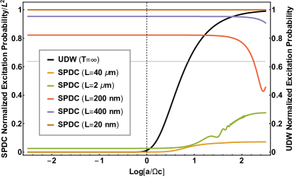
Figure 2: Normalized detector excitation probabilities. For the UDW detector (black line), we plot $2\pi\Omega/(a(\exp(2\pi\Omega/a)-1)$, which has a Planckian form in $\Omega$ with a temperature $\beta^{-1}=a/2\pi$. For the SPDC system (coloured lines), we plot $|\mathcal{A}^{\prime}_{\textsc{s}}/\tilde{\kappa}\tilde{\eta}L|^{2}$. For longer crystals, the curve is qualitatively similar to the Planckian curve while for shorter crystals, the excitation probability decreases with acceleration (this was also observed in brenna2016anti , and may be related to the anti-Unruh effect garay2016thermalization ). For comparison, we plot $2/\pi$ (horizontal dashed line), which is the normalized excitation probability/$L^{2}$ for a standard periodically-poled crystal (periodicity $\Lambda\approx 3.5~{}\mu$m) of length $L$ phasematched at $\omega_{1}=\Omega_{1}$ and $\omega_{2}=\Omega_{2}$.

Group velocity dispersion (GVD) can be engineered, e.g., by varying the cross-sectional shape and area of the waveguide ahmad2018modeling or by varying the distance between coupled cavities in a photonic crystal slab fussell2007engineering . There may exist a material or parameter regime where realistic GVD variations will lead to reasonable count rates, but finding these will require an extensive parameter search (made complicated by the need to integrate highly-oscillating functions), as well as extension of the analysis to three-dimensional waveguides. We leave this for future work.

In the mean-time, the analogy between the acceleration of a UDW detector and the relative dispersion raises interesting questions. Is it possible to use GVD engineering as a new approach to phase matching? On the other hand, how should one think about the analogue of periodic poling—a common quasi-phasematching technique in NLO— in the context of a UDW detector? And how does the analogy introduced in this paper relate to the analogy between the refractive index of a dielectric and curvature of spacetime novello2002artificial ? These would be interesting to explore further.

The Unruh effect lies at the intersection of thermal physics, quantum physics and gravity. It’s an important signpost in the search for the theory of quantum gravity earman2011unruh ; smolin2008three . Unfortunately, the effect is yet to be verified experimentally. While simulations of some Unruh-related phenomena have been studied in various systems, including NLO, this is the first proposal for simulating an Unruh-DeWitt detector using optical modes and a nonlinear material. We expect this analogy to be fruitful in the cross-pollination of ideas among different areas of physics.

III Acknowledgements

AMB thanks Eduardo Martín-Martínez and Robb Mann for helpful discussions. Research at Perimeter Institute is supported by the Government of Canada through Industry Canada and by the Province of Ontario through the Ministry of Research and Innovation. This research was supported in part by the Natural Sciences and Engineering Research Council of Canada (RGPIN-2016-04135), Canada Research Chairs, Industry Canada and the Transformative Quantum Technologies program.

Appendix A The Unruh-DeWitt transition amplitude

We now compute $\bra{\omega}\phi(x(\tau)t(\tau))\ket{0}$, where $\ket{\omega}=a^{\dagger}(\omega)\ket{0}$:

$$\bra{\omega}\phi(x(\tau)t(\tau))\ket{0}={} \bra{0}a^{\dagger}(\omega)\left(\int\frac{d\omega_{k}}{\sqrt{4\pi\omega_{k}}}(a(\omega_{k})e^{-i\omega_{k}q(\tau)}+a^{\dagger}(\omega_{k})e^{i\omega_{k}q(\tau)})\right)\ket{0}$$ (11)

$$={} \int\frac{d\omega_{k}}{\sqrt{4\pi\omega_{k}}}(e^{-i\omega_{k}q(\tau)}\bra{0}a^{\dagger}(\omega)a(\omega_{k})\ket{0}+e^{i\omega_{k}q(\tau)}\bra{0}a^{\dagger}(\omega)a^{\dagger}(\omega_{k})\ket{0})$$ (12)

$$={} \int\frac{d\omega_{k}}{\sqrt{4\pi\omega_{k}}}e^{-i\omega_{k}q(\tau)}\delta(\omega-\omega_{k})$$ (13)

$$={} \frac{e^{-i\omega q(\tau)}}{{\sqrt{4\pi\omega}}}\,.$$ (14)

Therefore the amplitude for transition from the ground state $|g,0\rangle$ to the state $|e,\omega\rangle$ (where $g$ and $e$ represent the ground and excited states of the detector respectively; and $0$ and $k$ represent the ground and single-photon-excited states of the field) at first order expansion of the evolution operator is:

$$\mathcal{A}_{\textsc{u},\omega}(\Omega)={} -i\bra{e,\omega}\int_{\tau_{i}}^{\tau_{f}}\mathrm{d}\tau H_{\textsc{u}}(\tau)\ket{g,0}$$ (15)

$$={} -i\bra{e,\omega}\int_{\tau_{i}}^{\tau_{f}}\mathrm{d}\tau\lambda\eta(\tau)m(\tau)\phi(x(\tau),t(\tau))\ket{g,0}$$ (16)

$$={} -i\int_{\tau_{i}}^{\tau_{f}}\mathrm{d}\tau\lambda\eta(\tau)\bra{e}m(\tau)\ket{g}\bra{\omega}\phi(x(\tau),t(\tau))\ket{0}$$ (17)

$$={} -\frac{i\lambda\mathcal{M}}{\sqrt{4\pi\omega_{k}}}\int_{\tau_{i}}^{\tau_{f}}\mathrm{d}\tau\eta(\tau)e^{-i\omega q(\tau)}\,,$$ (18)

with $\mathcal{M}=\langle e|m(\tau)|g\rangle=\bra{e}e^{iH_{0}\tau}m(0)e^{-iH_{0}\tau}\ket{g}=\bra{e}m(0)\ket{g}e^{i\Omega\tau}$. This can then be written as

$$\mathcal{A}_{\textsc{u},\omega}(\Omega)={} b(\omega_{k})\int_{\tau_{i}}^{\tau_{f}}\mathrm{d}\tau\eta(\tau)e^{i\Omega\tau}e^{-i\omega q(\tau)}\,,$$ (19)

where $b(\omega)=-i\lambda/\sqrt{4\pi\omega}\bra{e}m(0)\ket{g}$.

Appendix B The SPDC transition amplitude

The interaction Hamiltonian for a three-wave mixing process in a waveguide is given in yang2008spontaneous as:

$$\begin{split}H_{{}_{\textsc{s}}}(t)={}&\frac{1}{3\epsilon_{0}}\int d\mathbf{r}\Gamma^{ijk}_{(2)}(\mathbf{r})\hat{D}^{i}(\mathbf{r},t)\hat{D}^{j}(\mathbf{r},t)\hat{D}^{k}(\mathbf{r},t)\,,\end{split}$$ (20)

where $\Gamma^{ijk}_{(2)}(\mathbf{r})$ is a tensor related to the more commonly-used nonlinear tensor $\chi^{ijk}_{(2)}(\mathbf{r})$ via Eq. (15) in yang2008spontaneous , and $D^{i/j/k}$ are the quantized displacement field operators. Under the assumptions that the tensor nature of $\chi_{(2)}(\mathbf{r})$ and the vector nature of the mode profiles of the displacement field can be neglected, $\chi_{(2)}$ can be taken to characterize the strength of the nonlinearity. Let us assume that we have three fields present in the process (labelled by $j=1,2,3$), which all have zero overlap with each other, either due to non-overlapping frequencies or orthogonal polarization. Let us also assume that the fields propagate collinearly along $z$ through a waveguide of length $L$ with only one transverse mode that is uniform over a cross-sectional area $A$. Furthermore, let us assume that one of the fields ($j=3$) is intense, non-depleting, and can be treated classically. The interaction Hamiltonian can then be written as (see Eq. (3.28) of quesada2015very ):

$$\begin{split}H_{{}_{\textsc{s}}}(t)={}&-\hbar\epsilon\int_{0}^{\infty}d\omega_{1}\int_{0}^{\infty}d\omega_{2}\int_{0}^{\infty}d\omega_{3}~{}e^{i(\omega_{1}+\omega_{2}-\omega_{3})t}~{}\mathrm{sinc}\left(\frac{L}{2}\left(k_{1}(\omega_{1})+k_{2}(\omega_{2})-k_{3}(\omega_{3})\right)\right)\\ &\times\alpha(\omega_{3})\hat{a}^{\dagger}_{1}(\omega_{1})\hat{a}^{\dagger}_{2}(\omega_{2})+\text{H.c.}\end{split}$$ (21)

where $k_{j}(\omega)=\omega n_{j}(\omega)/c$, where $n_{j}(\omega)$ is the refractive index of mode $j$, where

$$\epsilon=2L\chi^{(2)}\sqrt{\frac{\sqrt{2}U_{0}\pi\Omega_{1}\Omega_{2}}{\sqrt{\pi}(4\pi)^{3}\epsilon_{0}Ac^{3}n_{1}(\Omega_{1})n_{2}(\Omega_{2})n_{3}(\Omega_{3})\tau}}\,,$$ (22)

where $\Omega_{j}$ are the central frequencies of the fields, $U_{0}$ is the energy of the classical pulse used to pump the crystal and

$$\alpha(\omega_{3})=\frac{\tau}{\sqrt{\pi}}e^{-\tau^{2}(\omega_{3}-\Omega_{3})^{2}}$$ (23)

is the shape of the pulse, which has units of time, where $\tau=1/\sqrt{\sigma}=2\sqrt{2\ln 2}\quad\mathrm{FWHM}$, where $\sigma$ is the standard deviation of the Gaussian distribution in frequency, and FWHM is the full width at half maximum of a Gaussian distribution.

We now generalize this result to include a spatial dependence on the nonlinear susceptibility. It is not necessary to repeat the derivation from quesada2015very from first principles for the general case. We can just reverse some of the final steps in that derivation and make our generalizations at the appropriate points. We first note that

$$\chi^{(2)}\mathrm{sinc}\left(\frac{L}{2}\left(k_{1}(\omega_{1})+k_{2}(\omega_{2})-k_{3}(\omega_{3})\right)\right)=\frac{1}{L}\int_{z_{i}}^{z_{f}}dz\chi^{(2)}e^{-i(k_{1}(\omega_{1})+k_{2}(\omega_{2})-k_{3}(\omega_{3}))z}\,,$$ (24)

where $z_{i}=-L/2$ and $z_{f}=L/2$, and then make the substitution $\chi^{(2)}\rightarrow\chi^{(2)}(z)$. We also include a spatial dependence on the refractive index by making the substitution $n_{j}(\omega)\rightarrow n_{j}(\omega;z)$, which in turn requires the substitution

$$(k_{1}(\omega_{1})+k_{2}(\omega_{2})-k_{3}(\omega_{3}))z\rightarrow\int_{z_{i}}^{z}d\zeta(k_{1}(\omega_{1};\zeta)+k_{2}(\omega_{2};\zeta)-k_{3}(\omega_{3};\zeta))\,,$$ (25)

where the integral over $\zeta$ keeps track of the phase picked up as the light propagates through a material with variable $k_{j}$ helmfrid1993influence ; santandrea2019fabrication .

The interaction Hamiltonian becomes

$$\begin{split}H_{{}_{\textsc{s}}}(t)={}&-\frac{\hbar\kappa}{2\pi}\int_{0}^{\infty}d\omega_{1}\int_{0}^{\infty}d\omega_{2}\int_{0}^{\infty}d\omega_{3}~{}e^{i(\omega_{1}+\omega_{2}-\omega_{3})t}\alpha(\omega_{3})\hat{a}^{\dagger}_{1}(\omega_{1})\hat{a}^{\dagger}_{2}(\omega_{2})\\ &\times\int_{z_{i}}^{z_{f}}dz\frac{\chi^{(2)}(z)}{\sqrt{n_{1}(\Omega_{1};z)n_{2}(\Omega_{2};z)n_{3}(\Omega_{3};z)}}e^{-i\int_{-L/2}^{z}d\zeta(k_{1}(\omega_{1};\zeta)+k_{2}(\omega_{2};\zeta)-k_{3}(\omega_{3};\zeta))}+\text{H.c.}\end{split}$$ (26)

where

$$\kappa=4\pi\sqrt{\frac{\sqrt{2}U_{0}\pi\Omega_{1}\Omega_{2}}{\sqrt{\pi}(4\pi)^{3}\epsilon_{0}Ac^{3}\tau}}\,.$$ (27)

We now use this Hamiltonian to derive the transition amplitude in Eq. (3). We start with the definition in Eq. (6) and insert the expression for the Hamiltonian in Eq. (26), to give

$$\begin{split}\mathcal{A}_{\textsc{s}}={}&i\frac{\kappa}{2\pi}\int_{-\infty}^{\infty}\mathrm{d}t\int_{0}^{\infty}d\omega_{3}~{}e^{i(\omega+\Omega_{2}-\omega_{3})t}\alpha(\omega_{3})\\ &\times\int_{z_{i}}^{z_{f}}dz\frac{\chi^{(2)}(z)}{\sqrt{n_{1}(\Omega_{1};z)n_{2}(\Omega_{2};z)n_{3}(\Omega_{3};z)}}e^{-i\int_{-L/2}^{z}d\zeta(k_{1}(\omega;\zeta)+k_{2}(\Omega_{2};\zeta)-k_{3}(\omega_{3};\zeta))}\,.\end{split}$$ (28)

If we now perform the integral over time, we get

$$\begin{split}\mathcal{A}_{\textsc{s}}={}&i\kappa\int_{0}^{\infty}d\omega_{3}~{}\delta(\omega+\Omega_{2}-\omega_{3})\alpha(\omega_{3})\\ &\times\int_{z_{i}}^{z_{f}}dz\frac{\chi^{(2)}(z)}{\sqrt{n_{1}(\Omega_{1};z)n_{2}(\Omega_{2};z)n_{3}(\Omega_{3};z)}}e^{-i\int_{-L/2}^{z}d\zeta(k_{1}(\omega;\zeta)+k_{2}(\Omega_{2};\zeta)-k_{3}(\omega_{3};\zeta))}\,,\end{split}$$ (29)

and perform the integral over $\omega_{3}$ to give

$$\mathcal{A}_{\textsc{s}}={} i\kappa\alpha(\Omega_{2}+\omega)\int_{z_{i}}^{z_{f}}dz\frac{\chi^{(2)}(z)}{\sqrt{n_{1}(\Omega_{1};z)n_{2}(\Omega_{2};z)n_{3}(\Omega_{3};z)}}e^{-i\int_{-L/2}^{z}d\zeta\Delta k(\Omega_{2},\omega;\zeta)}\,,$$ (30)

where $\Delta k(\Omega_{2},\omega;\zeta)=k_{1}(\omega;\zeta)+k_{2}(\Omega_{2};\zeta)-k_{3}(\Omega_{2}+\omega;\zeta)$.

The pump laser is centred at frequency $\Omega_{3}$. We can then take $\alpha(\Omega_{2}+\omega)$ to be a function of $\omega$ centred about $\omega=\Omega_{1}=\Omega_{3}-\Omega_{2}$, and assume that $\Delta k(\Omega_{2},\omega;\zeta)$ is close to linear in $\omega$ where $\alpha(\Omega_{2}+\omega)$ is non-negligible. We then do a first-order expansion of $\Delta k(\Omega_{2},\omega;\zeta)$ about $\omega=\Omega_{1}$. The terms are

$$k_{1}(\omega;z)={} k_{1}(\Omega_{1};z)+\frac{1}{v_{1}(z)}(\omega-\Omega_{1})$$ (31a)

$$k_{2}(\Omega_{2};z)={} k_{2}(\Omega_{2};z)$$ (31b)

$$k_{3}(\Omega_{2}+\omega;z)={} k_{3}(\Omega_{3};z)+\frac{1}{v_{3}(z)}(\omega-\Omega_{1})\,.$$ (31c)

where $v_{1}(z)=(\partial k_{1}(\omega;z)/\partial\omega|_{\omega=\Omega_{1}})^{-1}$ and $v_{3}(z)=(\partial k_{3}(\Omega_{2}+\omega;z)/\partial\omega|_{\omega=\Omega_{1}})^{-1}$ are the group velocities for modes 1 and 3. Using $\Omega_{1}=\Omega_{3}-\Omega_{2}$, we can write $\Delta k(\Omega_{2},\omega;z)$ as

$$\Delta k(\Omega_{2},\omega;z)=\Delta k_{0}(z)-\frac{1}{\Delta v_{g}(z)}(\Omega_{3}-\Omega_{2})+\frac{1}{\Delta v_{g}(z)}\omega\,,$$ (32)

where

$$\Delta k_{0}(z)={} k_{3}(\Omega_{3};z)-k_{2}(\Omega_{2};z)-k_{1}(\Omega_{1};z)$$ (33)

is the phase mismatch, and

$$\frac{1}{\Delta v_{g}(z)}={} \frac{1}{v_{3}(z)}-\frac{1}{v_{1}(z)}$$ (34)

is the relative inverse group velocity. We now identify

$$\Delta k(\Omega_{2},\omega_{s};z)=\underbrace{\Delta k_{0}(z)-\frac{1}{\Delta v_{g}(z)}(\Omega_{3}-\Omega_{2})}_{\tilde{\Omega}(z)}+\underbrace{\frac{1}{\Delta v_{g}(z)}}_{\frac{d}{dz}\tilde{q}(z)}\omega\,.$$ (35)

With all of this, we can then write

$$\mathcal{A}_{\textsc{s}}={} b_{\textsc{s}}(\omega)\int_{z_{i}}^{z_{f}}dz\tilde{\eta}(z)e^{i\tilde{\Omega}(z)z}e^{i\omega\tilde{q}(z)}\,,$$ (36)

where

$$b_{\textsc{s}}(\omega)={} i\kappa\alpha(\Omega_{2}+\omega)$$ (37a)

$$\tilde{\Omega}(z)={} \Delta k_{0}(z)-\frac{1}{\Delta v_{g}(z)}(\Omega_{3}-\Omega_{2})$$ (37b)

$$\tilde{\eta}(z)={} \frac{\chi^{(2)}(z)}{\sqrt{n_{1}(\Omega_{2}+\Omega_{3};z)n_{2}(\Omega_{2};z)n_{3}(\Omega_{3};z)}}$$ (37c)

$$\tilde{q}(z)={} \int_{z_{i}}^{z}\frac{1}{\Delta v_{g}(\zeta)}d\zeta\,.$$ (37d)

References

• (1) William G Unruh. Notes on black-hole evaporation. Physical Review D, 14(4):870, 1976.
• (2) SW Hawking and W. Israel. General relativity, 1979.
• (3) William G Unruh and Robert M Wald. What happens when an accelerating observer detects a rindler particle. Physical Review D, 29(6):1047, 1984.
• (4) John Earman. The unruh effect for philosophers. Studies In History and Philosophy of Science Part B: Studies In History and Philosophy of Modern Physics, 42(2):81–97, 2011.
• (5) Daniel F Walls and Gerard J Milburn. Quantum optics. Springer Science & Business Media, 2007.
• (6) Thomas G Philbin, Chris Kuklewicz, Scott Robertson, Stephen Hill, Friedrich König, and Ulf Leonhardt. Fiber-optical analog of the event horizon. Science, 319(5868):1367–1370, 2008.
• (7) TLM Guedes, Matthias Kizmann, Denis V Seletskiy, Alfred Leitenstorfer, Guido Burkard, and Andrey S Moskalenko. Spectra of ultrabroadband squeezed pulses and the finite-time unruh-davies effect. Physical review letters, 122(5):053604, 2019.
• (8) Petr O Fedichev and Uwe R Fischer. Gibbons-hawking effect in the sonic de sitter space-time of an expanding bose-einstein-condensed gas. Physical review letters, 91(24):240407, 2003.
• (9) Petr O Fedichev and Uwe R Fischer. Observer dependence for the phonon content of the sound field living on the effective curved space-time background of a bose-einstein condensate. Physical Review D, 69(6):064021, 2004.
• (10) GS Paraoanu. Recent progress in quantum simulation using superconducting circuits. Journal of Low Temperature Physics, 175(5-6):633–654, 2014.
• (11) Javier Rodríguez-Laguna, Leticia Tarruell, Maciej Lewenstein, and Alessio Celi. Synthetic unruh effect in cold atoms. Physical Review A, 95(1):013627, 2017.
• (12) Jiazhong Hu, Lei Feng, Zhendong Zhang, and Cheng Chin. Quantum simulation of unruh radiation. Nature Physics, page 1, 2019.
• (13) Raúl Carballo-Rubio, Luis J Garay, Eduardo Martín-Martínez, and José de Ramón. Unruh effect without thermality. Physical review letters, 123(4):041601, 2019.
• (14) Paul M Alsing, David McMahon, and GJ Milburn. Teleportation in a non-inertial frame. Journal of Optics B: Quantum and Semiclassical Optics, 6(8):S834, 2004.
• (15) S Jay Olson and Timothy C Ralph. Entanglement between the future and the past in the quantum vacuum. Physical Review Letters, 106(11):110404, 2011.
• (16) Mariona Aspachs, Gerardo Adesso, and Ivette Fuentes. Optimal quantum estimation of the unruh-hawking effect. Physical review letters, 105(15):151301, 2010.
• (17) Wilson G Brenna, Robert B Mann, and Eduardo Martín-Martínez. Anti-unruh phenomena. Physics Letters B, 757:307–311, 2016.
• (18) Luis J Garay, Eduardo Martín-Martínez, and José de Ramón. Thermalization of particle detectors: The unruh effect and its reverse. Physical Review D, 94(10):104048, 2016.
• (19) M. O. Scully and Zubairy M. S. Quantum Optics. Cambridge University Press, 1997.
• (20) Peter W Milonni. The quantum vacuum: an introduction to quantum electrodynamics. Academic press, 2013.
• (21) L Sriramkumar and T Padmanabhan. Finite-time response of inertial and uniformly accelerated unruh-dewitt detectors. Classical and Quantum Gravity, 13(8):2061, 1996.
• (22) Pieter Kok, W. J. Munro, Kae Nemoto, T. C. Ralph, Jonathan P. Dowling, and G. J. Milburn. Linear optical quantum computing with photonic qubits. Rev. Mod. Phys., 79(1):135, 2007.
• (23) Nicolas Gisin and Rob Thew. Quantum communication. Nat Photon, 1(3):165–171, March 2007.
• (24) John M Donohue, Michael D Mazurek, and Kevin J Resch. Theory of high-efficiency sum-frequency generation for single-photon waveform conversion. Physical Review A, 91(3):033809, 2015.
• (25) B. L. Higgins, D. W. Berry, S. D. Bartlett, H. M. Wiseman, and G. J. Pryde. Entanglement-free Heisenberg-limited phase estimation. Nature, 450(7168):393–396, 2007.
• (26) T. Nagata, R. Okamoto, J. L. O’Brien, K. Sasaki, and S. Takeuchi. Beating the Standard Quantum Limit with Four-Entangled Photons. Science, 316(5825):726, 2007.
• (27) G. Brida, M. Genovese, and Ruo BercheraI. Experimental realization of sub-shot-noise quantum imaging. Nat Photon, 4(4):227–230, 04 2010.
• (28) Agedi N. Boto, Pieter Kok, Daniel S. Abrams, Samuel L. Braunstein, Colin P. Williams, and Jonathan P. Dowling. Quantum interferometric optical lithography: Exploiting entanglement to beat the diffraction limit. Phys. Rev. Lett., 85(13):2733–2736, Sep 2000.
• (29) M.B. Nasr, S. Carrasco, B.E.A. Saleh, A.V. Sergienko, M.C. Teich, J.P. Torres, L. Torner, D.S. Hum, and M.M. Fejer. Ultrabroadband biphotons generated via chirped quasi-phase-matched optical parametric down-conversion. Physical review letters, 100(18):183601, 2008.
• (30) Zhenshan Yang, Marco Liscidini, and JE Sipe. Spontaneous parametric down-conversion in waveguides: a backward heisenberg picture approach. Physical Review A, 77(3):033808, 2008.
• (31) David CM Ostapchuk, Shih-Yuin Lin, Robert B Mann, and BL Hu. Entanglement dynamics between inertial and non-uniformly accelerated detectors. Journal of High Energy Physics, 2012(7):72, 2012.
• (32) Francesco Graffitti, Dmytro Kundys, Derryck T Reid, Agata M Brańczyk, and Alessandro Fedrizzi. Pure down-conversion photons through sub-coherence-length domain engineering. Quantum Science and Technology, 2(3):035001, 2017.
• (33) United Crystals. Properties of KTP/KTA Single Crystal. http://www.unitedcrystals.com/KTPProp.html. [Online; accessed 22 Aug. 2019].
• (34) H Ahmad, MR Karim, and BMA Rahman. Modeling of dispersion engineered chalcogenide rib waveguide for ultraflat mid-infrared supercontinuum generation in all-normal dispersion regime. Applied Physics B, 124(3):47, 2018.
• (35) David P Fussell and Marc M Dignam. Engineering the quality factors of coupled-cavity modes in photonic crystal slabs. Applied physics letters, 90(18):183121, 2007.
• (36) Mário Novello, Matt Visser, and Grigory E Volovik. Artificial black holes. World Scientific, 2002.
• (37) Lee Smolin. Three roads to quantum gravity. Basic books, 2008.
• (38) N Quesada. Very nonlinear quantum optics. PhD thesis, Ph. D. thesis (University of Toronto, 2015), 2015.
• (39) Sten Helmfrid, Gunnar Arvidsson, and Jonas Webjörn. Influence of various imperfections on the conversion efficiency of second-harmonic generation in quasi-phase-matching lithium niobate waveguides. JOSA B, 10(2):222–229, 1993.
• (40) Matteo Santandrea, Michael Stefszky, Vahid Ansari, and Christine Silberhorn. Fabrication limits of waveguides in nonlinear crystals and their impact on quantum optics applications. New Journal of Physics, 2019.