Why $\alpha_{s}$ Cannot be Determined from Hadronic Processes without Simultaneously Determining the Parton Distributions

We show that any determination of the strong coupling $\alpha_{s}$ from a process which depends on parton distributions, such as hadronic processes or deep-inelastic scattering, generally does not lead to a correct result unless the parton distributions (PDFs) are determined simultaneously along with $\alpha_{s}$. We establish the result by first showing an explicit example, and then arguing that the example is representative of a generic situation which we explain using models for the shape of equal $\chi^{2}$ contours in the joint space of $\alpha_{s}$ and the PDF parameters.

1 The determination of $\alpha_{s}$ in hadronic processes

The value of the strong coupling $\alpha_{s}$ has been routinely determined from a variety of processes which involve hadrons in the initial state, both in electroproduction and hadroproduction. The current PDG average [1] includes two different classes of such determinations. One is from “DIS and PDF fits”: in these determinations the value of $\alpha_{s}$ is determined together with a set of parton distributions (PDFs) from a more or less wide set of data and processes, ranging from deep-inelastic scattering (DIS) to hadron collider processes (such as Drell-Yan, top, and jet production).

The other is from single hadronic processes: specifically top pair production [2, 3, 4], and jet electroproduction [5]. Several more determinations of $\alpha_{s}$ from one process have been presented, such as for instance jet production [6, 7, 8, 9, 10, 11, 12, 13], multijets [7, 14, 15, 16, 17, 18, 19, 20, 21] and $W$ and $Z$ production [22]. In these determinations, PDFs are taken from a pre-existing set, rather than being determined along with $\alpha_{s}$. The value of $\alpha_{s}$ is then found by determining the likelihood of the new data as a function of $\alpha_{s}$ — crudely speaking, by computing the $\chi^{2}$ to the new data of the theoretical prediction which corresponds to a variety of values of $\alpha_{s}$, and determining the minimum of the parabola (though in practice when various parametric uncertainties have to be properly kept into account the procedure is rather more elaborate, see e.g. Ref. [3]). The theoretical prediction is in turn obtained for each value of $\alpha_{s}$ by combining the matrix element computed with the given $\alpha_{s}$ value with the PDF set that corresponds to that $\alpha_{s}$ value. This is of course necessary because PDFs strongly depend on $\alpha_{s}$, so a consistent calculation requires the use of PDFs corresponding to that value. All major PDF sets are available for a variety of $\alpha_{s}$ values, and thus this poses no difficulty in practice.

Here we will show that this apparently straightforward and standard procedure may lead to an incorrect determination of $\alpha_{s}$, and we will argue that this is in fact a generic situation. The difference between this and the true best fit $\alpha_{s}$ can be very substantial, and specifically much larger than the statistical accuracy of the $\alpha_{s}$ determination: as we shall see, this in fact reflects a conceptual flaw in the procedure.

The reason for this can be understood by viewing the $\chi^{2}$ as a simultaneous function of $\alpha_{s}$ and the PDF parameters. Any given existing PDF set then traces a line in such space (the “best-fit line”, henceforth): for each value of $\alpha_{s}$ there is a set of best-fit PDF parameters, which corresponds to a point in PDF space. The standard procedure seeks for the minimum of the $\chi^{2}$ in this subspace. This disregards the fact that the true minimum generally corresponds to a different point in (PDF, $\alpha_{s}$) space, which also accommodates the new data [23].

One could naively argue that the standard procedure is correct, because what one is really doing is determining the best $\alpha_{s}$ value for the new process subject to the constraint that PDFs describe well the (typically very large) set of data used to determine them. And surely – the naive argument goes — the minimum of $\alpha_{s}$ anywhere other than on the best-fit line must correspond to a worse description of the world data? It actually turns out that this is incorrect: there exist points in (PDF, $\alpha_{s}$) space for which the value of the $\chi^{2}$ for the new process is lower than any value along the best-fit line, yet, somewhat counter-intuitively, the value of the $\chi^{2}$ for the world data is also lower.

Moreover, the value of $\alpha_{s}$ corresponding to these configurations may, and in general will, differ substantially from the one obtained using the standard procedure, and in particular it will be closer to the value obtained by simultaneously fitting $\alpha_{s}$ and PDFs to a global dataset. Therefore, the standard procedure leads to a distorted answer, and it inflates artificially the dispersion of $\alpha_{s}$ values obtained from different processes.

We establish this result by first providing an explicit example in which this happens. Namely, we consider the dataset used for the NNPDF3.1 [24] PDF determination. We then study the $\chi^{2}$ for the subset of data corresponding to the $Z$ transverse-momentum ($p_{t}$) distribution, and determine the best-fit value of $\alpha_{s}$ from this $Z$ $p_{T}$ distribution along the best-fit line corresponding to the global fit dataset. We then exhibit a specific set of PDFs corresponding to a rather different value of $\alpha_{s}$, and such that the $\chi^{2}$ is better both for the $Z$ $p_{T}$ distribution, and for the rest of the dataset. This means that there exists at least one point in (PDF, $\alpha_{s}$) space such the value of the $\chi^{2}$ for the $Z$ $p_{T}$ is better than any value along the best-fit line, and that there is no reason not to consider this as a better fit than the result at the best-fit $\alpha_{s}$ along the best-fit line, because the agreement with the world data is also better than that at the minimum on the best-fit line.

We will understand the reason for this result by providing models for the shape of the $\chi^{2}$ contours both for the world data and the new experiment in the joint (PDF, $\alpha_{s}$) space. Specifically, we explain that this situation may arise both in the case in which the new data may provide an independent determination of $\alpha_{s}$ and the PDFs of its own, and in the case in which the new data do not determine $\alpha_{s}$ and the PDFs independently. This then covers the typical realistic scenarios in which the new data only constrain (or determine) a subset of PDFs: e.g. in the case of the $Z$ $p_{T}$ distribution considered above, the gluon. In this latter, common case we will see that the value of $\alpha_{s}$ obtained through the standard procedure leads to an artificially large dispersion of $\alpha_{s}$ values: better-fit points in (PDF, $\alpha_{s}$) generally lead to $\alpha_{s}$ values which are closer to the global best fit.

2 An explicit example: the $Z$ transverse momentum distribution

We provide an explicit example of the situation we described in the introduction. We consider the $\chi^{2}$ values for both a global “world” dataset, and the dataset for a particular process $P$, as a function of $\alpha_{s}$. Given a fixed value of $\alpha_{s}$, the value of $\chi^{2}$ also depends on the PDF set which is being used. As $\alpha_{s}$ is varied, there is a PDF set which corresponds to the global best fit: this PDF set defines a line in (PDF, $\alpha_{s}$) space which we call the best-fit line. We call $\chi^{2}_{g}(\alpha_{s})$ the value of the $\chi^{2}$ for the global dataset, as a function of $\alpha_{s}$, along this best-fit line.

We now consider the $\chi^{2}$ for process $P$: We denote by ${\chi^{r}_{P}}^{2}(\alpha_{s})$ the value of the $\chi^{2}$ for process $P$ as a function of $\alpha_{s}$, along this same best-fit line in (PDF, $\alpha_{s}$) space. We call this the restricted $\chi^{2}$ for process $P$. This means that this restricted ${\chi^{r}_{P}}^{2}(\alpha_{s})$ is found using the value $\alpha_{s}$ of the strong coupling, but the PDF set which corresponds to the global best fit. So $\chi^{2}_{g}(\alpha_{s})$ and ${\chi^{r}_{P}}^{2}(\alpha_{s})$ are determined using the same $\alpha_{s}$ and the same PDF set: that which corresponds to the global best fit. Note that, for any value of $\alpha_{s}$, this restricted ${\chi^{r}_{P}}^{2}(\alpha_{s})$ is not in general the lowest $\chi^{2}$ value for process $P$ that can be found with the given value $\alpha_{s}$ of the strong coupling — the PDFs are optimized for the global dataset, not for process $P$. This is unlike the global $\chi^{2}_{g}(\alpha_{s})$, in which (by definition) for each $\alpha_{s}$ choice, the PDF set is always chosen as the corresponding global best-fit PDF set.

Now, the standard procedure determines $\alpha_{s}$ from process $P$ as the minimum of ${\chi^{r}_{P}}^{2}(\alpha_{s})$: namely, as the value of $\alpha_{s}$ which minimizes $\chi^{r}_{P}$, the restricted $\chi^{2}$ for process $P$, evaluated along the best-fit line. We call this value of $\alpha_{s}$, determined using the standard procedure, ${\alpha_{0}^{r}}^{P}$: the restricted best-fit value of $\alpha_{s}$, and the corresponding PDF set the restricted best-fit PDF set for process $P$.

We now show that this restricted ${\alpha_{0}^{r}}^{P}$ cannot be viewed as the value of $\alpha_{s}$ determined by process $P$. We do this by exhibiting a point in (PDF, $\alpha_{s}$) space which does not lie along the best-fit line, i.e. such that the PDFs do not correspond to the global best fit, such that $\alpha_{s}\not={\alpha_{0}^{r}}^{P}$, and such that both the $\chi^{2}$ for the individual dataset, and for the global dataset, are respectively better than the restricted ${\chi^{r}_{P}}^{2}({\alpha_{0}^{r}}^{P})$ and $\chi^{2}_{\rm g}({\alpha_{0}^{r}}^{P})$. This is thus a better fit to both process $P$ and the global dataset than the restricted best fit, so there is no sense in which the restricted best-fit ${\alpha_{0}^{r}}^{P}$ — which would be the “standard” answer — can be considered the $\alpha_{s}$ value determined by process $P$.

Our construction is based on a previously published determination of $\alpha_{s}$ by the NNPDF collaboration [25], in which the strong coupling is determined together with a set of parton distributions based on a global dataset which is very close to that used for the NNPDF3.1 [24]. This $\alpha_{s}$ determination, which we now briefly summarize for completeness, builds upon the previous NNPDF methodology for PDF determination, in which PDFs are determined as a Monte Carlo set of PDF replicas, each of which is fitted to a replica of the underlying data. Note that, in this $\alpha_{s}$ determination, the PDFs and $\alpha_{s}$ are fitted simultaneously. This is unlike the case of previous determinations [26] in which PDFs were determined for a variety of $\alpha_{s}$ values, and then the best fit was sought by looking at the likelihood profile of the best fit as a function of $\alpha_{s}$. Whereas the two methodologies lead (if correctly implemented) to the same best-fit $\alpha_{s}$ value, simultaneous minimization ensures a more accurate determination of the uncertainty involved, as explained in Ref. [25], essentially because it determines the likelihood contours in (PDF, $\alpha_{s}$) space, rather than just the likelihood line corresponding to the best-fit PDF for each $\alpha_{s}$ value.

The way this is accomplished in Ref. [25] within the NNPDF methodology is by fitting each data replica several times for a number of different values of $\alpha_{s}$, thereby providing a correlated ensemble of PDF replicas, in which to each data replica corresponds a PDF replica for each value of $\alpha_{s}$. Namely, for the $k$-th data replica $D^{(k)}$, a PDF replica is found by determining the set of PDF parameters $\theta^{(k)}$ which minimize the $\chi^{2}$:

$$\theta^{(k)}(\alpha_{s}) =\mathrm{argmin}_{\theta}\left[\chi^{2}(\theta,D^{(k)},\alpha_{s})\right]\,,$$ (1)

where by $\mathrm{argmin}_{\theta}$ we mean that the minimization is performed with respect to $\theta$ for fixed $D^{(k)}$ and $\alpha_{s}$. It is then possible to compute the $\chi^{2}$ for the $k$-th data replica as $\alpha_{s}$ is varied:

$$\chi^{2(k)}(\alpha_{s})=\chi^{2}\left(\alpha_{s},\theta^{(k)}(\alpha_{s}),D^{(k)}\right)\,.$$ (2)

We thus find an ensemble of parabolas $\chi^{2(k)}(\alpha_{s})$, one for each data replica. The best-fit $\alpha_{s}$ for the $k$-th data replica corresponds to the minimum along the $k$-th parabola:

$$\alpha_{s}^{(k)}=\mathrm{argmin}\left[\chi^{2(k)}(\alpha_{s})\right].$$ (3)

In the NNPDF approach, the best-fit PDF value is the average of the PDF replica sample; similarly the best-fit $\alpha_{s}$ is determined averaging the $\alpha_{s}^{(k)}$ values. We refer to Ref. [25] for further details, specifically on the dataset. Here we will use the NNLO PDF replicas determined in that reference as our baseline.

We can now consider any particular process $P$ entering these global PDF determination, and ask ourselves what is the $\alpha_{s}$ value corresponding to process $P$. The “standard” answer would be to simply consider the ensemble of best-fit PDFs determined in the global fit, and compute again $\chi^{2(k)}(\alpha_{s})$ but now only including process $P$ in the computation of the $\chi^{2}$. We then get another set of parabolas

$${\chi^{r}}^{2(k)}_{P}(\alpha_{s})=\chi^{2}\left(\alpha_{s},\theta^{(k)}(\alpha_{s}),D_{P}^{(k)}\right)\ ,$$ (4)

where only the data $D_{P}$ for process $P$ have been used. Note that these are restricted $\chi^{2}$ parabolas, because the PDF parameters $\theta^{(k)}(\alpha_{s}),$ are those found in Eq. (1), by minimizing the global $\chi^{2}$. The minima

$${{\alpha^{r}_{s}}^{(k)}}_{P}=\mathrm{argmin}\left[{\chi_{P}^{r}}^{2(k)}(\alpha_{s})\right]$$ (5)

now give an ensemble of restricted best-fit $\alpha_{s}$ values for process $P$. Their average is then the restricted best fit for this process.

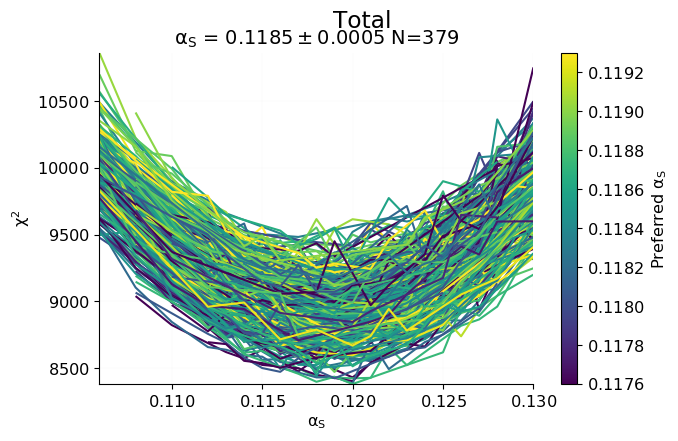
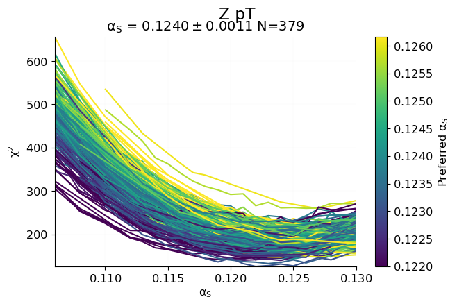
Figure 1: The $\chi^{2}$ profiles for each of the data replicas used for the NNLO determination of $\alpha_{s}(m_{Z})$ of Ref. [25]. Both the profiles for the total dataset (left), and for the $Z$ $p_{T}$ distribution (right) are shown.

In Fig. 1 we show the parabolas corresponding both to the global fit (left) and to the $Z$ $p_{T}$ distribution (right). The corresponding ensemble of values of $\alpha_{s}$ is shown in Fig. 2. From these we find that the global best-fit value of $\alpha_{s}(M_{Z})$ is

$$\alpha_{s}(M_{z})=\alpha_{0}^{g}=0.1185\pm 0.0005,$$ (6)

while the restricted best fit is, for the $Z$ $p_{T}$ distribution,

$$\alpha_{s}(M_{Z})={\alpha_{0}^{r}}^{Z\,p_{t}}=0.1240\pm 0.0015.$$ (7)

In both cases, the central value and uncertainty are respectively the mean and standard deviation computed over the replica sample, in the first cases for the global best fit Eq. (3) and in the latter case for the restricted best fit Eq. (5) for each replica.

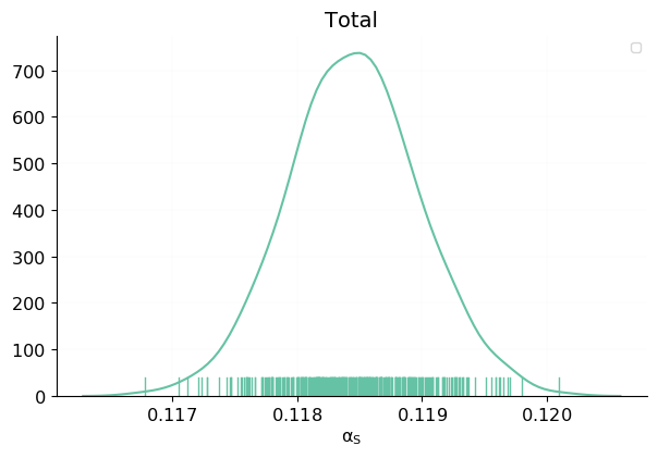
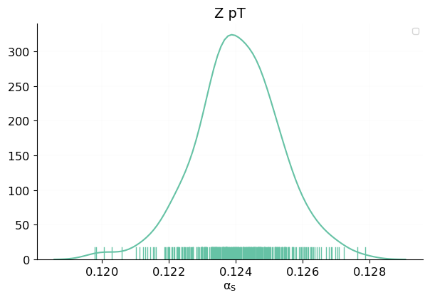
Figure 2: The probability distributions for the best-fit values $\alpha_{s}^{(k)}$ Eq. (3) and ${{\alpha_{s}^{r}}^{(k)}}_{P}$ Eq. (5) respectively for the global dataset (left) and the $Z$ $p_{T}$ distribution (right). Each marker indicates the value corresponding to each individual parabola of Fig. 1.

Dataset	$N_{\rm dat}$	default $\alpha_{s}=0.120$	reweighted $\alpha_{s}=0.120$	default $\alpha_{s}=0.124$
NMC	325	1.315	1.337	1.341
SLAC	67	0.6787	0.6994	0.7198
BCDMS	581	1.232	1.282	1.270
CHORUS	832	1.176	1.200	1.249
NuTeV dimuon	76	0.9229	0.9125	0.9900
HERA I+II inclusive	1145	1.263	1.271	1.288
HERA $\sigma_{c}^{\rm NC}$	37	1.533	1.538	1.748
HERA $F_{2}^{b}$	29	1.299	1.282	1.247
DY E866 $\sigma^{d}_{\rm DY}/\sigma^{p}_{\rm DY}$	15	1.019	1.020	1.048
DY E886 $\sigma^{p}$	89	0.4322	0.4221	0.4477
DY E605 $\sigma^{p}$	85	1.001	1.080	1.020
CDF $Z$ rap	29	1.442	1.558	1.419
D0 $Z$ rap	28	0.5990	0.6381	0.5996
D0 $W\to e\nu$ asy	8	2.794	2.860	2.979
D0 $W\to\mu\nu$ asy	9	1.594	1.610	1.629
ATLAS $W,Z$	30	0.8957	0.8912	0.9623
ATLAS high-mass DY 7 TeV	5	1.819	1.845	1.904
ATLAS low-mass DY 2011	6	1.123	1.060	1.605
ATLAS $W,Z$ 7 TeV 2011	34	2.149	1.889	2.289
ATLAS jets 2010 7 TeV	31	1.478	1.513	1.479
ATLAS $\sigma_{tt}^{\rm tot}$	3	0.8520	0.7088	3.503
ATLAS $t\bar{t}$ rap	10	1.555	1.339	2.214
CMS $W$ asy 840 pb	11	0.7858	0.7804	0.8083
CMS $W$ asy 4.7 fb	11	1.762	1.749	1.763
CMS Drell-Yan 2D 2011	110	1.264	1.332	1.294
CMS $W$ rap 8 TeV	22	1.010	1.068	1.177
CMS jets 7 TeV 2011	133	0.9766	1.026	1.034
CMS $\sigma_{tt}^{\rm tot}$	3	0.9832	0.5803	5.489
CMS $t\bar{t}$ rap	10	1.035	1.036	1.069
LHCb $Z$ 940 pb	9	1.595	1.773	1.568
LHCb $Z\to ee$ 2 fb	17	1.156	1.184	1.274
LHCb $W,Z\to\mu$ 7 TeV	29	1.793	2.034	1.894
LHCb $W,Z\to\mu$ 8 TeV	30	1.440	1.617	1.722
Global dataset	3979	1.212	1.235	1.262

Table 1: The values of $\chi^{2}/N_{\rm dat}$ for the experiments included in the best global fit with $\alpha_{s}=0.120$, compared to results obtained when $\alpha_{s}=0.124$, or when the $Z$ $p_{T}$ data are given a large weight and $\alpha_{s}=0.120$. The number of datapoints is also given in each case. The full description of the datasets, including data selection, cuts, and references is given in Ref. [24] where the same data coding is used.

We now show that the naive conclusion that the value Eq. (7) of $\alpha_{s}$ is the value of the strong coupling determined by the $Z$ $p_{T}$ distribution rests on shaky ground. To show it, we perform a new PDF determination in which the $Z$ $p_{T}$ are now given a large weight in the $\chi^{2}$, and which is otherwise identical to the default determination. This PDF determination is performed for a single value of $\alpha_{s}(M_{z})=0.120$, a value intermediate between the restricted best-fit ${\alpha_{0}^{r}}^{Z\,p_{t}}$ Eq. (7) and the global best-fit $\alpha_{0}^{g}$ Eq. (6). Specifically the contribution of the $Z$ $p_{T}$ data to the total $\chi^{2}$ has been multiplied by a factor $w=32$. This factor is chosen so that the contribution of the $Z$ $p_{T}$ data is roughly equal to that of all the other data. The gluon and total quark singlet PDFs obtained in this way are compared in Fig. 3 to the default PDFs for the same value of $\alpha_{s}(M_{Z})=0.120$; $\chi^{2}$ values for the global dataset are collected in Table 1, while in Table 2 $\chi^{2}$ values for the $Z$ $p_{T}$ data and the global dataset are compared. The gluon is shown because it is the PDF which is most affected by the $Z$ $p_{T}$ data, and the singlet is also shown because it mixes with the gluon upon perturbative evolution.

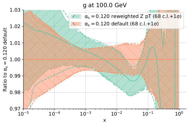
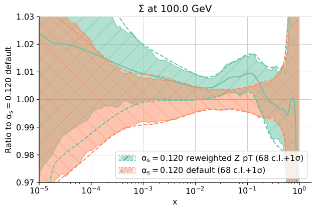
Figure 3: Comparison between the gluon (left) and quark singlet (right) PDFs in the default global PDF determination (orange, lower band at low $x$) and in a PDF determination in which the $Z$ $p_{T}$ data receive a large weight (green, higher band at low $x$), shown as a ratio to the former.

Dataset	$N_{\rm dat}$	default $\alpha_{s}=0.120$	default $\alpha_{s}=0.120$, no $Z$ $p_{T}$	reweighted $\alpha_{s}=0.120$	default $\alpha_{s}=0.124$
ATLAS $Z$ $p_{T}$ 8 TeV $(p_{T}^{ll},M_{ll})$	44	0.9776	0.9775	0.9380	0.9559
ATLAS $Z$ $p_{T}$ 8 TeV $(p_{T}^{ll},y_{ll})$	48	0.9999	1.071	0.7455	0.8568
CMS $Z$ $p_{T}$ 8 TeV $(p_{T}^{ll},M_{ll})$	28	1.308	1.299	1.403	1.357
All $Z$ $p_{T}$	120	1.056	1.085	0.9635	1.011
Global dataset	3979	1.212	1.211	1.235	1.262

Table 2: Same as Table 1, but now comparing the values of $\chi^{2}/N_{\rm dat}$ for the $Z$ $p_{T}$ distributions and the global dataset. The values for the global dataset are the same as in Table 1, while the values for the total $z$ $p_{T}$ are obtained by combining the three datasets listed in this table. We also include values for a global fit from which the $Z$ $p_{T}$ data have been excluded.

The logic behind this procedure is that by giving more weight to this data we obtain a set of PDFs which provide a better fit to them: so we expect the value of $\chi^{2}$ for the $Z$ $p_{T}$ data to be better than that which would be obtained by taking the default best-fit PDF set for the same $\alpha_{s}$ value. In fact it turns out that the value of the $\chi^{2}$ thus obtained for the $Z$ $p_{T}$ data is also better than the value ${\chi^{r}_{P}}^{P}(0.124)$ which corresponds to the best fit along the global best-fit line (see Table 2). This means that the value $\alpha_{s}(M_{Z})=0.120$ is a better fit to the $Z$ $p_{T}$ than the value Eq. (7) corresponding to the best fit along the best-fit line.

As discussed in the introduction one might object to the conclusion that $\alpha_{s}(M_{Z})=0.120$ might be a better $\alpha_{s}$ from $Z$ $p_{T}$: on the grounds that the PDF which we obtained thus are not compatible with the rest of the global dataset given that they do not correspond to the global best fit. However (see again Table 2) the value of $\chi^{2}$ for the global dataset obtained using these PDFs is also better than the value of ${\chi^{2}}_{\rm g}(0.124)$: hence with $\alpha_{s}(M_{Z})=0.120$ and these PDFs one gets a better fit to the $Z$ $p_{T}$ data than with $\alpha_{s}(M_{Z})=0.124$, while also better fitting the world data. As it is clear from Fig. 3, the PDFs that best reproduce the $Z$ $p_{T}$ data, though compatible within uncertainties with the global fit, differ from them by an amount which is sufficient to considerably improve the description of the $Z$ $p_{T}$ data. Indeed, they lead to an improvement of their $\chi^{2}$ value by almost 10% in comparison to that of the global fit with the same $\alpha_{s}(M_{Z})=0.120$ value, at the cost of only a small deterioration of the $\chi^{2}$ of the global fit, by about 2%.

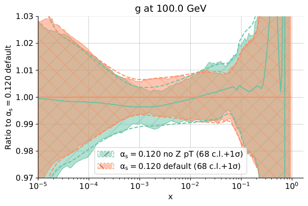
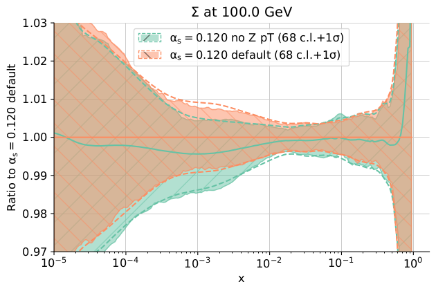
Figure 4: Same as Fig. 3, but now comparing the global fit (same as shown in Fig. 3) to a global fit from which the $Z$ $p_{T}$ data have been removed, shown as a ratio to the former.

The conclusion that the restricted best-fit value ${\alpha_{0}^{r}}^{{Z\,p_{t}}}$ Eq. (7) is the value of the strong coupling determined by the $Z$ $p_{T}$ distribution is thus difficult to defend: with $\alpha_{s}(M_{Z})=0.120$ we can fit better both the $Z$ $p_{T}$ and the global dataset, provided the PDFs are suitably readjusted. It is perhaps worth stressing that the effect that we are demonstrating is large in comparison to uncertainties. Indeed, the global best fit Eq. (6) differs by almost four standard deviations from the restricted best fit Eq. (7) in units of the large uncertainty on the latter. Assuming the same uncertainty, the better-fit value $\alpha_{s}(M_{Z})=0.120$ would instead be compatible with the global best fit within uncertainties.

This result is at first surprising, as one might expect that the best fit to the world data must be along the best-fit line. However, as we we shall show shortly, it can be understood both at a qualitative, and also more quantitative level.

Note that the dataset for the global fit that we are considering actually does include the $Z$ $p_{T}$ data of Table 2. Hence, the example presented here differs somewhat from a standard “real-life” situation such as in Refs. [3]-[5]: there, PDFs obtained from a fit to a global dataset are used for an $\alpha_{s}$ determination from some new process which was not among those which were used to determine the PDFs. In practice, in our case, this makes essentially no difference because the inclusion of the $Z$ $p_{T}$ data has almost no effect on the global fit, due to relatively small number of data (about a hundred vs. about 4000, see Table 2), and because the $Z$ $p_{t}$ data are quite consistent with other data which determine the same PDFs (essentially the large $x$ gluon) [27]. This is demonstrated explicitly in Fig. 4, where PDFs in the global fit with or without $Z$ $p_{T}$ data are compared, and seen to be essentially identical. Also, $\chi^{2}$ values for a global fit in which the $Z$ $p_{T}$ data are not included are shown in Table 2, and are seen to be extremely close to those for the default global fit which includes this data: even the $\chi^{2}$ for the $Z$ $p_{T}$ data themselves are almost unchanged when fitting this data. We have checked that all $\chi^{2}$ values for the other datasets of Table 1 change at or below the permille level upon exclusion of the $Z$ $p_{T}$ data.

As we will discuss in Sect. 2 below, whether or not the data for process $P$ are included in the global fit or not also makes no difference of principle, though this is besides the point now, given the negligible impact of the $Z$ $p_{T}$ data on the global fit. The reason why we choose to use for process $P$ dataset which is part of the global dataset, is that it enables us to use the very large set of 8400 correlated replicas produced for Ref. [25] in order to construct the profiles shown in Fig. 1, thereby ensuring high statistical accuracy.

We conclude that we have presented an explicit example that shows how, using an existing PDF set to determine $\alpha_{s}$ from a particular process $P$ by looking for the minimum of the $\chi^{2}$ for the process along the best-fit line of the global fit, can lead to a substantially distorted result. The reason is that there exists values of $\alpha_{s}$ for which (for a suitable PDF configuration) the $\chi^{2}$ for process $P$ is lower than the minimum along the best-fit line, but, surprisingly, the $\chi^{2}$ of the global dataset is also lower than the value it has at the minimum along the best-fit line.

This apparently puzzling result can be qualitatively understood by noting that the value of $\alpha_{s}$ which optimizes the $\chi^{2}$ of the chosen process is actually closer to the global minimum for $\alpha_{s}$ than the value which corresponds to the minimum along the best-fit line. Due to having given large weight to some process, the $\chi^{2}$ for the global dataset deteriorates somewhat, because it is now optimized for that process, rather than for the global dataset. But that deterioration is more than compensated by the fact that the $\alpha_{s}$ value is now closer to the global minimum. This is a consequence of the fact that the PDF space is higher-dimensional (perhaps even infinite-dimensional) so a small distortion of the PDFs is sufficient to accommodate the highly weighted process, and consequently the global $\chi^{2}$ only increases by a small amount due to the reweighting. In the next section we cast this qualitative argument in a more quantitative form.

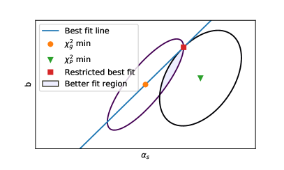
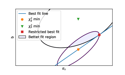
Figure 5: Likelihood ($\chi^{2}$) contours in (PDF, $\alpha_{s}$) space for toy models in which a given process $P$ is sufficient to determine PDFs; the parameter $b$ ($y$ axis) schematically represents the PDF parameters. The minimum of the global $\chi^{2}_{g}$ is the orange circle while the minimum of $\chi^{2}_{P}$ for process $P$ is the green triangle. The line is the locus of the best-fit PDF (“best-fit line”): the stationary value Eq. (9) of $b$ for the global $\chi^{2}$ for fixed $\alpha_{s}$. The red square is the restricted best-fit ${\alpha_{0}^{r}}^{P}$: the value of $\alpha_{s}$ corresponding to lowest restricted ${\chi^{r}_{P}}^{2}$, i.e. the point with lowest ${\chi_{P}^{2}}$ along the best-fit line. The ellipses are fixed $\chi^{2}_{P}$ and $\chi^{2}_{g}$ contours. The shaded area denotes the region in which both $\chi^{2}_{g}<\chi^{2}_{g}({\alpha_{0}^{r}}^{P})$ and $\chi^{2}_{P}<\chi^{2}_{P}({\alpha_{0}^{r}}^{P})$. The two plots correspond to two possible scenarios (see text).

3 The likelihood in (PDF, $\alpha_{s}$) space

We now discuss some models for the dependence of the likelihood profiles on $\alpha_{s}$ and the PDFs which explain the results which we found in the previous section, and show under which conditions the situation we encountered can be reproduced. Namely, we explicitly exhibit likelihood patterns for both a global dataset and a specific process $P$, such that there exist points in (PDF, $\alpha_{s}$) space which have a higher likelihood (lower $\chi^{2}$) than the restricted best fit — the point along the global best-fit line in (PDF, $\alpha_{s}$) space which maximizes the likelihood for process $P$. As in the previous section, we refer to (minus) the log-likelihood for the global dataset as $\chi^{2}_{g}$, and that for process $P$ as $\chi^{2}_{P}$.

We assume that the global dataset determines simultaneously the PDFs and $\alpha_{s}$, so that $\chi^{2}_{g}$ has a single minimum value in (PDF, $\alpha_{s}$) space, with fixed-$\chi^{2}_{g}$ ellipses about it. We then consider a particular subset of data, corresponding to a process $P$: the case of the $Z$ $p_{T}$ data discussed in the previous section is an explicit example, but one may consider both wider datasets (e.g., all LHC data), or smaller datasets (e.g., one particular measurement of some cross-section performed by one experiment).

We further distinguish two broad classes of cases. The first, which is more common, is that process $P$ does not fully determine the PDFs. This is the case of the $Z$ $p_{T}$ data of the previous section, which constrain the gluon distribution in the medium-large $x$ range but otherwise have a limited impact (see in particular Sect. 4.2 of Ref. [24]). In this case, likelihood contours for process $P$ in (PDF, $\alpha_{s}$) space have flat directions, along which PDFs and $\alpha_{s}$ change but the value of $\chi^{2}_{P}$ does not. The second is that in which process $P$ alone is sufficient to provide a determination of the PDFs, so that $\chi^{2}_{P}$ also has a minimum in (PDF, $\alpha_{s}$) space, with fixed-$\chi_{P}^{2}$ ellipses about it. An explicit example of this would be if process $P$ was the full set of deep-inelastic scattering data, which do determine fully the PDFs, albeit with larger uncertainties than a global dataset [28]. This case is relatively less common, but we discuss it first because the former case can be viewed as a spacial case of the latter.

3.1 Datasets which determine simultaneously $\alpha_{s}$ and PDFs

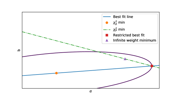
Figure 6: Same as Fig. 5, but now for a toy model in which process P does not fully determine the PDFs. The minimum of the global $\chi^{2}_{g}$ is the orange circle while the minimum of the $\chi^{2}_{P}$ for process $P$ is the dashed green line. The solid blue line is the best-fit line as in Fig. 5. The red square is the “standard” value ${\alpha_{0}^{r}}^{P}$: the value of $\alpha_{s}$ corresponding to lowest restricted ${\chi^{r}_{P}}^{2}$, i.e. the point with lowest ${\chi_{P}^{2}}$ along the best-fit line. The ellipse is a fixed $\chi_{g}^{2}$ contour.

In order to simplify the discussion, we consider a toy model in which the whole of PDF space is represented by a single parameter $b$ so that (PDF, $\alpha_{s}$) space is just the two-dimensional ($b$, $\alpha_{s}$) plane. In a realistic situation, this can be viewed as a two-dimensional cross-section of the full space. In the vicinity of the minimum, where the $\chi^{2}$ behaves quadratically, likelihood contours are just ellipses (see Fig. 5):

$$\chi_{i}^{2}(b,\alpha_{s})=\left[\sigma^{i}_{1}[(\alpha_{s}-\alpha_{0}^{i})\cos\theta_{i}+(b-b_{0}^{i})\sin\theta_{i})]\right]^{2}+\left[\sigma^{i}_{2}[-(\alpha_{s}-\alpha_{0}^{i})\sin\theta_{i}+(b-b_{0}^{i})\cos\theta_{i})]\right]^{2},$$ (8)

where $i=g,\>P$ according to whether one is considering the global dataset, or the dataset for process $P$. In our toy model we neglect the higher-order cubic and quartic terms that would arise far from the minimum. The point $(b_{0}^{g},\alpha_{0}^{g})$ (denoted by an orange circle in Fig. 5) corresponds to the maximum likelihood for the global dataset, and the point $(b_{0}^{P},\alpha_{0}^{P})$ for process $P$.

The best-fit line defined in Section 2 is the locus of points such that

$$\frac{\partial\chi^{2}_{g}}{\partial b}(b,\alpha_{s})=0,$$ (9)

shown in Fig. 5 as a (blue solid) line. The condition Eq. (9) means that at each point along this line the tangent to the fixed-$\chi^{2}_{g}$ contour is vertical. Hence, the line is not a principal axis of the ellipse, unless the principal axes are along the $b$ and $\alpha_{s}$ directions. The restricted best-fit point is shown as a red square. This point, $(b^{r},{\alpha_{0}^{r}}^{P})$, minimizes the restricted ${\chi^{r}_{P}}^{2}$ along the best-fit line, so it is tangent to a fixed $\chi^{2}_{P}$ contour. This is the value of $\alpha_{s}$ from process $P$ that would be determined using the “standard” procedure. The value of $\chi^{2}$ for process $P$ at this point is the value discussed in Section. 2: ${\chi^{r}_{P}}^{2}({\alpha_{0}^{r}}^{P})\equiv\chi^{2}_{P}(b^{r},{\alpha_{0}^{r}}^{P})$.

The fixed $\chi^{2}_{g}$ and $\chi^{2}_{P}$ contours through the restricted best-fit point are also shown in figure. It is clear than, whenever they intersect, the whole area bounded by them (shown as shaded in the figure) has both $\chi^{2}_{g}<\chi_{g}^{2}(b^{r},{\alpha_{0}^{r}}^{P})$ and $\chi^{2}_{P}<\chi^{2}_{P}(b^{r},{\alpha_{0}^{r}}^{P})$. Any point in this region provides a better fit to both the global dataset and to process $P$. Whereas it is debatable which $\alpha_{s}$ value in this region (if any) should be considered as the best-fit value of $\alpha_{s}$, it seems very difficult to argue that the restricted best-fit ${\alpha_{0}^{r}}^{P}$ is the $\alpha_{s}$ value preferred by process $P$, given that it gives a worse fit to the both process $P$, and the global dataset than any point in the highlighted region.

The two toy examples shown in Fig. 5 demonstrate different cases in which this may happen. Clearly, for some choices of parameters the value of the restricted best-fit ${\alpha_{0}^{r}}^{P}$ might considerably differ from either of the values $\alpha_{0}^{P}$ or $\alpha_{0}^{g}$ that respectively minimize $\chi^{2}_{P}$ or $\chi^{2}_{g}$. In fact, one can exhibit situations, such as shown in the right plot of Fig. 5, in which $\alpha_{0}^{P}\approx\alpha_{0}^{g}$, yet the restricted best-fit ${\alpha_{0}^{r}}^{P}$ is quite different. So not only does the restricted best fit provide a worse fit, but it cannot even be viewed as some kind of average or interpolation between the global value $\alpha_{0}^{g}$ and the process $P$ value $\alpha_{0}^{P}$. This demonstrates that taking ${\alpha_{0}^{r}}^{P}$ as the value of $\alpha_{s}$ determined by process $P$ leads to an incorrect result.

3.2 Datasets which do not fully determine the PDFs

We now turn to the case in which process $P$ does not fully determine the PDFs, so that there are flat directions for $\chi^{2}_{P}$ in (PDF, $\alpha_{s}$) space. This means that, whereas the likelihood profile for the global dataset still has the form of Eq. (8), for process $P$ there exists a hypersurface in (PDF, $\alpha_{s}$) space (i.e. in our toy model a curve in the $(b,\alpha_{s})$ plane) along which $\chi^{2}_{P}$ is at a minimum. This can be viewed as a limiting case of Eq. (8), when the fixed $\chi_{P}^{2}$ ellipses become infinitely thin, i.e., when either of $\sigma^{P}_{i}$ goes to zero. Of course, just like far enough from the minimum the fixed-$\chi^{2}$ profile will no longer be ellipsoids, the flat direction will only be locally straight. This situation is depicted in Fig. 6, where the minimum curve for $\chi^{2}_{P}$ is shown as a (dashed, green) straight line. In this case, in the generic situation in which this minimum curve and the best-fit line Eq. (9) intersect, the intersection point is the restricted best fit $(b^{r},{\alpha_{0}^{r}}^{P})$, which would provide the “standard” $\alpha_{s}$ determination.

However, it is clear that if one now considers the fixed $\chi^{2}_{g}$ contour through this point (shown as the ellipse in Fig. 6) in a generic case, i.e. unless the minimum curve (the dashed green curve of Fig. 6) is tangent to this ellipse, the contour intercepts a segment of the minimum curve, and any point along this segment provides a better fit to the global dataset than the restricted best-fit $(b^{r},{\alpha_{0}^{r}}^{P})$. The minimum of the global $\chi^{2}_{g}$ along this segment is shown as a purple triangle in Fig. 6. Clearly, this is the point that is selected by minimizing the weighted

$$\chi^{2}_{w}=\chi^{2}_{g}+w\chi^{2}_{P}$$ (10)

in the limit of very large $w$. Indeed, in the limit in which $w$ is very large so $w\chi^{2}_{P}\gg\chi^{2}_{g}$ the minimum of $\chi^{2}_{w}$ is along the line of degenerate minima of $\chi^{2}_{P}$, but for any finite $w$ the absolute minimum of $\chi^{2}_{w}$ is at the point at which $\chi^{2}_{g}$ is also minimal.

Arguably, the value of $\alpha_{s}$ at this large-weight minimum can be viewed as the best-fit value $\alpha_{0}^{P}$ of $\alpha_{s}$ as determined from process $P$, subject to the constraint of also fitting the global dataset. Be that as it may, the best-fit value of $\alpha_{s}$ as determined from process $P$ is surely not the restricted best-fit ${\alpha_{0}^{r}}^{P}$, which leads to a worse fit to the global dataset than any value of $\alpha_{s}$ along the intercept segment.

This is then representative of the case that we discussed in the Section 2. On the one hand, the value ${\alpha_{0}^{r}}^{P}$ does not generically provide the best simultaneous fit of process $P$ and the global dataset. Also, the value that minimizes the weighted $\chi^{2}$ for large $w$ — which provides a better fit to the global dataset while giving a fit of the same quality to process $P$ — is generally closer to the global best-fit $\alpha_{0}^{g}$, as it is clear from Fig. 6. Note that in this simple example, in which PDF space is one-dimensional, the large-$w$ minimum leads to the same fit quality for process $P$ as the restricted minimum. In a realistic situation both flat and non-flat directions will be present, and the weighting will also change the position of the minimum along the non-flat direction, thereby leading to a lower $\chi^{2}$ for process $P$ than the restricted minimum, as we observed in Section 2.

We conclude that the situation we encountered in Section 2 is generic. Whenever process $P$ does not fully determine the PDFs, $\chi^{2}_{P}$ in (PDF, $\alpha_{s}$) space has a subspace of degenerate minima. The value of $\alpha_{s}$ obtained by minimizing the restricted ${\chi^{r}_{P}}^{2}$ then leads to an incorrect result, generally further away from the global best-fit $\alpha_{0}^{g}$ than the value that would be obtained by looking for the minimum of the global $\chi^{2}_{g}$ in this subspace of degenerate minima of $\chi^{2}_{P}$.

It is important to note that this effect can be quite large, as it was the case in the explicit example of the previous section. In general, the size of the deviation of the infinite weight minimum from the restricted minimum will depend on the numerical values of the parameters that characterize $\chi^{2}_{g}$ and $\chi^{2}_{P}$ Eq. (8). Note however that whenever the restricted best fit differs considerably from the global best fit in units of the standard deviation of the global best fit, then the $\chi^{2}_{g}$ parabola will vary rapidly in the vicinity of the restricted best fit, and thus the infinite weight minimum will generically have a rather different value. This is the case of the example of Section 2, in which the restricted minimum Eq. (7) is eleven standard deviations away from the global minimum Eq. (6). It is interesting to observe that in the recent determination of $\alpha_{s}$ [24] many of the restricted minima from individual datasets indeed differ considerably from the global minimum.

As a final observation, we note that the argument presented here, and thus its conclusion, are unaffected regardless of whether process $P$ is or is not included in the global dataset. This has the interesting implication that in a global simultaneous determination of $\alpha_{s}$ and the PDFs, such as performed in Ref. [25], the minimum of $\chi^{2}$ from each dataset entering the global determination cannot be interpreted as the $\alpha_{s}$ value corresponding to that dataset. Hence, there is no reason to expect that the global best-fit $\alpha_{s}$ is the mean of the restricted best-fit values determined from each subset of the data entering the global fit.

4 The value of $\alpha_{s}$ from a single process

The main conclusion of this paper is that it is generally not possible to reliably determine $\alpha_{s}$ from a given physical process which depends on parton distributions while relying on a pre-existing PDF set. The reason can be simply stated: the existing PDF sets only sample a line in PDF space as $\alpha_{s}$ is varied, hence, when using them, one is determining a constrained likelihood of the physical process under investigation along this line. This biases the results of the determination, in that the true maximum likelihood $\alpha_{s}$ generally corresponds to a PDF configuration which is not along this line. The bias is especially severe since PDF space is high-dimensional. We have proven our point by showing that there exist PDFs which provide a better fit both to the given process, and the global dataset, and correspond to a different $\alpha_{s}$ value. This has been shown both in an explicit example, and in toy models. Interestingly, when the physical process under investigation does not fully determine the PDFs, we have shown that this bias will generically pull the value of $\alpha_{s}$ away from the best fit, in comparison to values of $\alpha_{s}$ which provide a better fit to both the given process and the global dataset. Hence, determining $\alpha_{s}$ from individual processes in this way, artificially inflates the dispersion of the $\alpha_{s}$ values which are found.

It is important to stress that the problem that we are pointing out cannot be viewed as an extra source of PDF uncertainty in a determination which uses a pre-existing PDF set, but rather, it exposes a conceptual flaw. Indeed, the value of $\alpha_{s}$ found by not fitting the PDF simultaneously does not correspond to a maximum likelihood point in (PDF, $\alpha_{s}$) space, and as such it can differ from the true maximum likelihood point by an amount which is potentially large (as we have shown in explicit examples), and impossible to quantify without knowledge of the PDF dependence of the results.

One may then ask: what is the value of $\alpha_{s}$ determined by process $P$? Does it exist at all? Clearly, in the case in which the dataset for process $P$ is wide enough that it can be used to simultaneously determine both $\alpha_{s}$ and the PDFs, it is this value of $\alpha_{s}$ which must be interpreted as the value preferred by process $P$. In this case, the main import of our analysis is to show that minimizing along the line of global best-fit PDFs may lead to a value of $\alpha_{s}$ which not only provides a poor fit to both process $P$ and the global dataset, but cannot even be viewed as some kind of average of the value $\alpha_{0}^{P}$ from process $P$ and the global value $\alpha_{0}^{g}$; rather, it will randomly differ from them in a way which depends on the $\chi^{2}$ profiles in (PDF, $\alpha_{s}$) space (see the right plot in Figure 5).

On the other hand, it is very common that the process $P$ is insufficient to simultaneously determine $\alpha_{s}$ and the PDFs, and hence for $\chi^{2}_{P}$ to have a set of degenerate minima in (PDF, $\alpha_{s}$) space. In this case it is debatable whether it makes sense to speak of a value of $\alpha_{s}$ determined by process P. One may take the purist attitude that such value does not exist, or, alternatively consider defining the best fit value of $\alpha_{s}$ as the result of the weighting procedure discussed in in Section 3.2, i.e., as the best fit to the global dataset within the set of degenerate minima of the $\chi^{2}_{P}$. In such case, the uncertainty on this $\alpha_{s}$ value is determined by conventional one-$\sigma$ contours of the global $\chi^{2}$ in the degenerate subspace (i.e., in the example of Fig. 6, along the dashed green line).

The important observation in this case is that the value found minimizing along the best-fit line will generally be further away from the global best fit, while providing a worse fit to both process $P$ and the global dataset. So in particular if one wishes to assess the spread of values of $\alpha_{s}$ which are individually favored by each of the individual processes which enter in a global simultaneous determination of PDFs and $\alpha_{s}$ (such as that of Ref. [25]) a realistic estimate is found by weighting each of the individual datasets in turn, while the spread of the restricted minima will suggest an artificially inflated dispersion of values.

The upshot of this whole discussion is that we do not envisage a shortcut: a determination of $\alpha_{s}$ from a single process always requires a simultaneous determination of PDFs. In the simplest case, of a process (such as deep-inelastic scattering) which is sufficient to determine the PDFs, one must perform a simultaneous fit of the PDFs and $\alpha_{s}$ to the dataset for that process. In the more common case of a process which does not fully determine the PDFs one may determine a value of $\alpha_{s}$ for this process (if deemed interesting) through the weighting method discussed above, but this of course requires performing anyway a global PDF fit: so it is no easier than simply including process $P$ in the dataset and repeating the global simultaneous determination of the PDFs and $\alpha_{s}$.

In this latter case, of performing a global fit of PDFs and $\alpha_{s}$, it might at least in principle be possible to include the new dataset, without refitting, by Bayesian reweighting[29, 30]. Indeed, there is no difficulty of principle in reweighhting correlated replicas: each replica will then correspond not only to a different set of PDFs, but also to a different $\alpha_{s}$ value (that given by Eq. 3). The reweighted replica ensemble then also gives a posterior distribution of $\alpha_{s}$ values. Whether and how the procedure would work when the new dataset is given a large weight is however not immediately clear. Also, whether this is feasible in practice of course remains to be seen: specifically, it might well be that in concrete cases an unrealistically large number of replicas in the prior set is necessary in order to get a reliable answer after reweighting.

Our results have two wider sets of implications. On the one hand, they provide a strong indication that looking at the $\chi^{2}$ profile for any given process in the subspace of global fits as one parameter is varied can be very misleading. This is true not only for $\alpha_{s}$ but for any parameter entering the global fit, including the parameters which govern the shape of the PDF themselves. Specifically, the dispersion of best-fit minima for individual processes as a feature of the PDF is varied – such as, say, the rate at which the gluon grows at small $x$ – does not appear to be a good proxy of the actual dispersion of the results favored by each processes. This may have some relevance in the benchmarking of parton distributions (see e.g. Refs. [31, 32]).

On the other hand, they suggest caution in the determination of any standard model parameter from hadronic processes. Indeed, while the case of the determination of $\alpha_{s}$ is particularly relevant because of the very strong correlation of $\alpha_{s}$ and the PDFs, similar considerations apply to the simultaneous determination of any physical parameter in PDF-dependent processes, such as the determination of the top quark mass mass [33], or of electroweak parameters, such as the $W$ mass [34]. In the latter case, the correlation of PDFs and the parameter is in principle weaker than in the case of the strong coupling, but the very high accuracy which is sought suggest that currently available results, specifically in $W$ mass determination, should be reconsidered with care.

References

- [1] Particle Data Group Collaboration, M. Tanabashi et al., Review of Particle Physics, Phys. Rev. D98 (2018), no. 3 030001, [ http://pdg.lbl.gov/2019/reviews/rpp2019-rev-qcd.pdf]. Updated in 2019.
- [2] CMS Collaboration, S. Chatrchyan et al., Determination of the top-quark pole mass and strong coupling constant from the t t-bar production cross section in pp collisions at = 7 TeV, Phys.Lett. B728 (2014) 496, [arXiv:1307.1907].
- [3] T. Klijnsma, S. Bethke, G. Dissertori, and G. P. Salam, Determination of the strong coupling constant from measurements of the total cross section for top-antitop quark production, Eur. Phys. J. C77 (2017), no. 11 778, [arXiv:1708.07495].
- [4] CMS Collaboration, A. M. Sirunyan et al., Measurement of the production cross section, the top quark mass, and the strong coupling constant using dilepton events in pp collisions at 13 TeV, Eur. Phys. J. C79 (2019), no. 5 368, [arXiv:1812.10505].
- [5] H1 Collaboration, V. Andreev et al., Determination of the strong coupling constant in next-to-next-to-leading order QCD using H1 jet cross section measurements, Eur. Phys. J. C77 (2017), no. 11 791, [arXiv:1709.07251].
- [6] D. Britzger, K. Rabbertz, D. Savoiu, G. Sieber, and M. Wobisch, Determination of the strong coupling constant from inclusive jet cross section data from multiple experiments, arXiv:1712.00480.
- [7] H1 Collaboration, V. Andreev et al., Measurement of multijet production in collisions at high and determination of the strong coupling , Eur. Phys. J. C75 (2015), no. 2 65, [arXiv:1406.4709].
- [8] CMS Collaboration, V. Khachatryan et al., Measurement and QCD analysis of double-differential inclusive jet cross sections in pp collisions at TeV and cross section ratios to 2.76 and 7 TeV, JHEP 03 (2017) 156, [arXiv:1609.05331].
- [9] CDF Collaboration, T. Affolder et al., Measurement of the Strong Coupling Constant from Inclusive Jet Production at the Tevatron Collider, Phys. Rev. Lett. 88 (2002) 042001, [hep-ex/0108034].
- [10] ZEUS Collaboration, S. Chekanov et al., Jet-radius dependence of inclusive-jet cross-sections in deep inelastic scattering at HERA, Phys. Lett. B649 (2007) 12–24, [hep-ex/0701039].
- [11] D0 Collaboration, V. M. Abazov et al., Determination of the strong coupling constant from the inclusive jet cross section in collisions at sqrt(s)=1.96 TeV, Phys. Rev. D80 (2009) 111107, [arXiv:0911.2710].
- [12] B. Malaescu and P. Starovoitov, Evaluation of the Strong Coupling Constant Using the ATLAS Inclusive Jet Cross-Section Data, Eur. Phys. J. C72 (2012) 2041, [arXiv:1203.5416].
- [13] CMS Collaboration, V. Khachatryan et al., Constraints on parton distribution functions and extraction of the strong coupling constant from the inclusive jet cross section in pp collisions at TeV, Eur. Phys. J. C75 (2015), no. 6 288, [arXiv:1410.6765].
- [14] ATLAS Collaboration, G. Aad et al., Measurement of transverse energy-energy correlations in multi-jet events in collisions at TeV using the ATLAS detector and determination of the strong coupling constant , Phys. Lett. B750 (2015) 427–447, [arXiv:1508.01579].
- [15] ATLAS Collaboration, M. Aaboud et al., Determination of the strong coupling constant from transverse energy-energy correlations in multijet events at TeV using the ATLAS detector, arXiv:1707.02562.
- [16] ATLAS Collaboration, M. Aaboud et al., Measurement of dijet azimuthal decorrelations in collisions at TeV with the ATLAS detector and determination of the strong coupling, Phys. Rev. D98 (2018), no. 9 092004, [arXiv:1805.04691].
- [17] ZEUS Collaboration, S. Chekanov et al., Multijet production in neutral current deep inelastic scattering at HERA and determination of alpha(s), Eur. Phys. J. C44 (2005) 183–193, [hep-ex/0502007].
- [18] CMS Collaboration, S. Chatrchyan et al., Measurement of the Ratio of the Inclusive 3-Jet Cross Section to the Inclusive 2-Jet Cross Section in pp Collisions at = 7 TeV and First Determination of the Strong Coupling Constant in the TeV Range, Eur. Phys. J. C73 (2013), no. 10 2604, [arXiv:1304.7498].
- [19] D0 Collaboration, V. M. Abazov et al., Measurement of angular correlations of jets at TeV and determination of the strong coupling at high momentum transfers, Phys. Lett. B718 (2012) 56–63, [arXiv:1207.4957].
- [20] CMS Collaboration, V. Khachatryan et al., Measurement of the inclusive 3-jet production differential cross section in proton–proton collisions at 7 TeV and determination of the strong coupling constant in the TeV range, Eur. Phys. J. C75 (2015) 186, [arXiv:1412.1633].
- [21] H1 Collaboration, V. Andreev et al., Measurement of Jet Production Cross Sections in Deep-inelastic ep Scattering at HERA, Eur. Phys. J. C77 (2017), no. 4 215, [arXiv:1611.03421].
- [22] D. d’Enterria and A. Poldaru, Strong coupling extraction from a combined NNLO analysis of inclusive electroweak boson cross sections at hadron colliders, arXiv:1912.11733.
- [23] Z. Kassabov, PDF dependence on parameter fits from hadronic data, Acta Phys. Polon. Supp. 11 (2018) 329, [arXiv:1802.05236].
- [24] NNPDF Collaboration, R. D. Ball et al., Parton distributions from high-precision collider data, Eur. Phys. J. C77 (2017), no. 10 663, [arXiv:1706.00428].
- [25] NNPDF Collaboration, R. D. Ball, S. Carrazza, L. Del Debbio, S. Forte, Z. Kassabov, J. Rojo, E. Slade, and M. Ubiali, Precision determination of the strong coupling constant within a global PDF analysis, Eur. Phys. J. C78 (2018), no. 5 408, [arXiv:1802.03398].
- [26] R. D. Ball, V. Bertone, L. Del Debbio, S. Forte, A. Guffanti, et al., Precision NNLO determination of using an unbiased global parton set, Phys.Lett. B707 (2012) 66–71, [arXiv:1110.2483].
- [27] E. R. Nocera and M. Ubiali, Constraining the gluon PDF at large x with LHC data, PoS DIS2017 (2018) 008, [arXiv:1709.09690].
- [28] S. Forte, Z. Kassabov, J. Rojo, and L. Rottoli, ”Theoretical Uncertainties and Dataset Dependence of Parton Distributions”, in Proceedings of the 2017 Les Houches workshop ’Physics at TeV colliders”, .
- [29] W. T. Giele and S. Keller, Implications of hadron collider observables on parton distribution function uncertainties, Phys. Rev. D58 (1998) 094023, [hep-ph/9803393].
- [30] The NNPDF Collaboration, R. D. Ball et al., Reweighting NNPDFs: the W lepton asymmetry, Nucl. Phys. B849 (2011) 112–143, [arXiv:1012.0836].
- [31] R. D. Ball, S. Carrazza, L. Del Debbio, S. Forte, J. Gao, et al., Parton Distribution Benchmarking with LHC Data, JHEP 1304 (2013) 125, [arXiv:1211.5142].
- [32] J. R. Andersen et al., Les Houches 2013: Physics at TeV Colliders: Standard Model Working Group Report, arXiv:1405.1067.
- [33] S. Alekhin, S. Moch, and S. Thier, Determination of the top-quark mass from hadro-production of single top-quarks, Phys. Lett. B763 (2016) 341–346, [arXiv:1608.05212].
- [34] E. Bagnaschi and A. Vicini, A new look at the estimation of the PDF uncertainties in the determination of electroweak parameters at hadron colliders, arXiv:1910.04726.