Experimental demonstration of sequential quantum random access codes

Abstract

A random access code (RAC) is a strategy to encode a message into a shorter one in a way that any bit of the original can still be recovered with nontrivial probability. Encoding with quantum bits rather than classical ones can improve this probability but has an important limitation: Due to the disturbance caused by standard quantum measurements, qubits cannot be used more than once. However, as recently shown by Mohan, Tavakoli, and Brunner [New J. Phys. 21 083034 (2019)], weak measurements can alleviate this problem, allowing two sequential decoders to perform better than with the best classical RAC. We use single photons to experimentally show that these weak measurements are feasible and nonclassical success probabilities are achievable by two decoders. We prove this for different values of the measurement strength and use our experimental results to put tight bounds on them, certifying the accuracy of our setting. This proves the feasibility of using sequential quantum RACs for quantum information tasks such as the self-testing of untrusted devices.

I INTRODUCTION

A random access code (RAC) is a communication protocol that requires a transmitter (Alice) to encode a $n-$bit long random sequence into a shorter $m-$bit message, and a receiver (Bob) to be able to decode any of the $n$ bits with non-trivial probability $p>1/2$. These parameters are often grouped in expression $n\xrightarrow{p}m$ that describes the task. A quantum random access code (QRAC) is the very similar situation in which Alice sends $m$ qubits rather than bits. This concept was introduced by Wiesner Wiesner (1983) but caught the interest of the scientific community only after subsequent research by Ambainis et al. Ambainis et al. (1999) who showed quantum strategies that achieve $2\xrightarrow{0.85}1$ and $3\xrightarrow{0.78}1$, which beat the best classical RACs for these choices of $n,m$. Further studies found that a $4\rightarrow 1$ QRAC that reaches $p>1/2$ does not exist Hayashi et al. (2006) but a $4^{m}-1\rightarrow m$ always does Iwama et al. (2007). Other investigations considered different values of $n,m$ Nayak (1999), the use of qudits ($d-$level quantum systems) rather than qubits Casaccino et al. (2008); Tavakoli et al. (2015); Liabøtrø (2017), or the request of decoding more than 1 bit Ben-Aroya et al. (2008). Applications include communication complexity Klauck (2001), network coding Hayashi et al. (2007), locally decodable codes Kerenidis and de Wolf (2004), dimension witnessing of quantum states Wehner et al. (2008), self-testing of quantum devices Tavakoli et al. (2018); Farkas and Kaniewski (2019), semi-device-independent quantum randomness extraction (SDI-QRE) Li et al. (2012); Lunghi et al. (2015); Li et al. (2015), and semi-device-independent key distribution (SDI-QKD) Pawłowski and Brunner (2011); Chaturvedi et al. (2018).

Recently, improvements in the theory and implementation of weak and sequential quantum measurements Aharonov et al. (1988); Mitchison et al. (2007); Schiavon et al. (2017); Li et al. (2018); An et al. (2018); Chen et al. (2019); Foletto et al. (2019), prompted the introduction of sequential QRACs by Mohan, Tavakoli, and Brunner [(MTB) in what follows] Mohan et al. (2019). Their protocol is a variation of the $2\rightarrow 1$ QRAC: Alice encodes a two-bit message into 1 qubit and sends it to Bob, who, after measuring it, forwards the resulting quantum state to a third party (Charlie) who shares the same goal as Bob: decoding any of the two bits of Alice with nontrivial probability $p>1/2$. The core tenets of quantum physics remind us that Bob’s measurement disturbs the initial state, making it more difficult for Charlie to extract information from it. However, if Bob uses weak measurements rather than projective ones, he can tune this disturbance and give back some information to Charlie at the cost of some of his own. This means that Alice’s qubit can be used more than once, overcoming a crucial limit of previously studied QRACs, but there is a trade-off between Bob’s and Charlie’s attainable information that depends on Bob’s measurement strength. The observation of decoding probabilities that saturate this trade-off self-tests the use of a unique set of states and measurements under the assumption that states are two dimensional and measurements have binary outcomes. Additionally, even imperfect results can bind Bob’s measurement strength. This can be important for the characterization of untrusted quantum devices.

In this paper, we verify MTB’s protocol in a quantum optics experiment for different values of the strength parameter. We show that it is possible to observe near-optimal decoding probabilities and we put tight bounds on Bob’s strength using MTB’s self-testing expressions. Finally, we discuss some applications of these results.

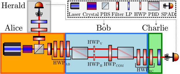
Figure 1: Scheme of the experimental setup. The sequences of three half-wave plates (HWPs) before and after the Mach-Zehnder interferometer (MZI) are implemented with a single plate each, but we show them here to better separate the roles of Alice, Bob, and Charlie. The arrow indicates that Bob and Charlie only observe the outcome when the detectors click.

II MODEL

We briefly introduce the quantitative relations presented by MTB and add some comments. Let $x=(x_{0},x_{1})\in\{0,1\}^{2}$ be the two-bit sequence that Alice wants to encode. Let $y$ and $z\in\{0,1\}$ label the positions of the bit in $x$ that Bob and Charlie randomly choose, respectively, to decode. Finally, let $b$ and $c$ be the results of Bob and Charlie’s respective measurements, associating bit 0 with outcome $+1$ and bit 1 with $-1$. We define the two correlation witnesses,

$$W_{AB} =\frac{1}{8}\sum_{x,y}p(b=x_{y}|x,y),$$ (1)

$$W_{AC} =\frac{1}{8}\sum_{x,z}p(c=x_{z}|x,z),$$ (2)

which quantify the probabilities that Bob and Charlie correctly decode the bit they are interested in, averaged over all possible input sequences and bit choices.

If the parties use classical physics, these probabilities are independent of each other and limited by $W_{AB},W_{AC}\leq\frac{3}{4}$. This upper bound is reached, for example, if Alice sends the first of her bits, meaning that when Bob and Charlie want to decode the second, they can only guess. Yet, MTB found that the two decoders can both violate this limit in a quantum scenario. The aforementioned trade-off between the information that each of them can extract translates into an upper bound to $W_{AC}$ that depends on the attained value of $W_{AB}$. In particular,

$$W_{AC}\leq\frac{1}{8}\left(4+\sqrt{2}+\sqrt{16W_{AB}-16W_{AB}^{2}-2}\right),$$ (3)

with $W_{AB}$ itself being limited by previous results at $W_{AB}\leq\frac{1}{2}+\frac{\sqrt{2}}{4}$ Ambainis et al. (1999). MTB also proposed a strategy to saturate this trade-off and proved that it is unique up to unitary transformations and under the assumption that Alice’s state is two dimensional and all measurements have binary outcomes. This strategy reads

1. Alice encodes her two-bit sequence $x=(x_{0},x_{1})$ into one of four pure states and sends it to Bob. These states form the angles of a square in the $XZ$ equatorial line of the Bloch sphere and are equidistant from the eigenstates of $\sigma_{X}$ and $\sigma_{Z}$: $\varrho_{x}=\frac{1}{2}\left[\mathbb{1}+(-1)^{x_{0}}\frac{\sigma_{X}}{\sqrt{2}}+(-1)^{x_{1}}\frac{\sigma_{Z}}{\sqrt{2}}\right]$.

2. Bob weakly measures $\sigma_{X}$ if $y=0$ or $\sigma_{Z}$ if $y=1$ on the qubit, with strength parameter labeled $\eta\in[0,1]$ as in Ref. Mohan et al. (2019). The first case ($y=0$) entails using the two-outcome positive operator-valued measure (POVM) $\left(M_{b|0},b\in\{0,1\}\right)$ where $M_{b|0}=\frac{1}{2}\left[\mathbb{1}+(-1)^{b}\eta\sigma_{X}\right]$. The state is transformed according to Kraus operator $K_{b|0}=\frac{1}{2}[(\cos{\mu}+\sin{\mu})\mathbb{1}+(-1)^{b}(\cos{\mu}-\sin{\mu})\sigma_{X}]$, where $\mu=\frac{1}{2}\arccos(\eta)$. In this way, $K_{0|0}^{\dagger}K_{0|0}-K_{1|0}^{\dagger}K_{1|0}=M_{0|0}-M_{1|0}=\eta\sigma_{X}$. The second case ($y=1$) is similar with $\sigma_{X}$ replaced by $\sigma_{Z}$. Bob then sends the resulting state to Charlie.

3. Charlie performs projective measurements of $\sigma_{X}$ if $z=0$ or $\sigma_{Z}$ if $z=1$.

In this situation, the following relations hold:

$$W_{AB} =\frac{1}{2}+\frac{\sqrt{2}}{4}\eta,$$ (4)

$$W_{AC} =\frac{1}{2}+\frac{\sqrt{2}}{4}\left(\frac{1+\sqrt{1-\eta^{2}}}{2}\right),$$ (5)

which, when combined, make Expression (3) an equality. Notably, at least one of these witnesses is always above the classical limit of $\frac{3}{4}$ and if $\eta\in\left[\frac{1}{\sqrt{2}},\sqrt{2\sqrt{2}-2}\right]$ both are. For $\eta=\frac{4}{5}$, they take the same value of $\frac{1}{2}+\frac{\sqrt{2}}{5}$.

However, we add that this strategy cannot be straightforwardly extended to a third decoder. Even if Charlie also uses weak measurements with strength $\eta^{\prime}$ and relays the resulting qubit to David, there are no values of $(\eta,\eta^{\prime})$ that provide correlation witnesses greater than $\frac{3}{4}$ for all three decoders. We show this in Appendix A finding similar results to those attained in the context of the Clauser-Horne-Shimony-Holt inequality Mal et al. (2016).

One can wonder whether MTB’s protocol can improve the decoding probability of the entire input sequence. In a communication scenario in which Bob and Charlie cooperate and agree to always decode different bits, the joint probability of both being correct follows the law:

$$W_{ABC} =\frac{1}{8}\sum_{x,y}p(b=x_{y},c=x_{z}|x,y,z\neq y)$$ (6)

$$=\frac{1}{4}\left(1+\frac{\eta+\sqrt{1-\eta^{2}}}{\sqrt{2}}\right).$$

It holds that $W_{ABC}\leq\frac{1}{2}$ with the bound being reached only for $\eta=\frac{1}{\sqrt{2}}$. This agrees with the limits present in the literature: a $m$-qubit system cannot make the decoding probability of a $n$-bit message better than $2^{m}/2^{n}$ (Nayak, 1999, Theorem 2.4.2).

The uniqueness of the strategy consisting of C1-C3 allows MTB to conclude that finding $W_{AB}$ and $W_{AC}$ correlated to saturate Expression (3) self-tests that the state preparation was that of C1 and the measurements were those of C2 and C3. This is an important result for protocols of SDI-QRE or SDI-QKD in which devices cannot be trusted, and their behavior can be checked only from the outcomes they provide. Moreover, even if the values of the witnesses are suboptimal, they still give a lower and an upper bound on parameter $\eta$,

$$\eta \geq\eta_{low}=\sqrt{2}\left(2W_{AB}-1\right),$$ (7)

$$\eta \leq\eta_{up}=2\sqrt{\left(2+\sqrt{2}-4W_{AC}\right)\left(2W_{AC}-1\right)},$$ (8)

which become tight when conditions C1-C3 are fulfilled. These bounds can also be extended to self-tests on the incompatibility between Bob’s measurements Anwer et al. (2020), which is a crucial resource for many quantum information tasks. For instance, $W_{AB}$ and $W_{AC}$ can be used as self-tests for the characterization of the QKD state decoders even if the optimal conditions are not reached.

Finally, we add that trade-off (3) and its inverse,

$$W_{AB}\leq\frac{1}{2}\left[1+\sqrt{4(4+\sqrt{2})W_{AC}-16W_{AC}^{2}-4-2\sqrt{2}}\right]$$ (9)

can provide a security bound in an adversarial scenario in which Alice and Charlie try to detect a man in the middle (Bob) or infer the properties of his actions. In particular, if $W_{AC}>\frac{1}{2}+\frac{\sqrt{2}}{5}\approx 0.783$, then $W_{AC}>W_{AB}$ (see Fig. 3), meaning that Alice and Charlie can extract a cryptographic key secure from Bob’s eavesdropping using a SDI-QKD protocol, such as that of Ref. Pawłowski and Brunner (2011). Compared to the one present in the latter, Eq. (9) is a tighter upper bound on $W_{AB}$ and, in turn, on the mutual information between the legitimate parties’ key and the eavesdropper’s. Therefore, the performance of the protocol would be increased, although, here, we have the additional assumption that Bob’s measurements have binary outcomes.

III METHOD

Our experiment aims at verifying all these relations and showing that it is feasible to meet conditions C1-C3 and find the optimal trade-off. We also use Eqs. (7) and (8) to bind the value of $\eta$. We choose single photons as our experimental platform and their polarization as the degree of freedom that encodes the information. We produce photon pairs at 808 nm through spontaneous parametric down-conversion using a periodically poled potassium titanyl phosphate crystal in a type-II collinear-phase-matching configuration, so that the generated state after the polarizing beam splitter (PBS) is $\ket{\psi}=\ket{H_{A}}\ket{V_{herald}}$ Calderaro et al. (2018). One photon of each pair is selected in the $\ket{V}$ polarization to filter out imperfections in state preparation and background light, and is sent to a single-photon avalanche diode (SPAD) detector. Its presence heralds the other photon of the pair which reaches the core of the setup.

This is divided into three stages that play the role of Alice, Bob, and Charlie as shown in Fig. 1. First, Alice changes the state from $\ket{H}=\operatorname{tr}_{herald}\left(\ket{\psi}\bra{\psi}\ket{V_{herald}}\bra{V_{herald}}\right)$ to one of the four optimal states of condition C1 using a pair of HWPs. Bob carries out the weak measurement with a MZI based on polarizing beam displacers [(PBDs), Thorlabs BD40]. A first PBD entangles polarization with the path qubit, then the two arms encounter one HWP each, HWP_H and HWP_V in Fig. 1 with axes at angles 0 and $\pi/4$ relative to the horizontal direction defined by $\ket{H}$. HWP_COM spans across both arms and sets the strength of the measurement through its angle $\theta=\frac{\pi-\arccos(\eta)}{4}$. A second PBD has the dual purpose of closing the interferometer and performing the measurement. It does this by selecting the outcome 0 and sending the corresponding photons to the one exit that continues to the rest of the setup where they meet a HWP at angle $\pi/4$. This MZI + HWP scheme implements $K_{0|0}$: Two more HWPs, one before and one after it, can be rotated to select the other outcome or change the measurement basis. This means that Bob’s apparatus observes one outcome at a time; extensions that allow observing both in separate exits, thus, performing a full measurement, are possible (see Appendix B) but beyond the scope of this experiment. Charlie’s measurements are projective, therefore, his setup consists of a fixed linear polarizer (LP) preceded by a HWP that selects one combination of basis and outcome at a time. To reduce the number of components, we replaced the two groups of three consecutive HWPs with a single HWP each, which is controlled by two parties (HWP_AB and HWP_BC in Fig. 1). Finally, light is coupled into a single-mode fiber and sent to a SPAD detector. Its electrical signals are correlated with those of the herald and coincidences (within a $\pm 1$-ns window) are counted for a fixed exposure time of 2 s. The total number of coincidences in this time and for each measurement choice is approximately $8\times 10^{3}$.

Our implementation represents a proof of principle demonstration of a QRAC without active random choice of preparation and measurements. Moreover, Bob and Charlie do not observe their outcomes independently, but only when the detectors at the end of the setup click. We iterate sequentially over all the possible configurations of preparation ($x$), measurement choice ($y,z$), and outcome ($b,c$) by rotating HWP_AB and HWP_BC, whose angles are listed in Table 1 (Appendix C). For each, we record the number of coincident counts. These are proportional to the joint probability of the outcomes selected by Bob and Charlie, and we use them to compute the conditional probabilities required by Eqs. (1) and (2) to find the correlation witnesses.

IV RESULTS

We measure $W_{AB}$ and $W_{AC}$ for 11 different values of the strength parameter, equally spaced in $[0,1]$. We use the HWP inside Bob’s MZI to set its value of $\eta_{set}$. All the results that we report here are extracted from the same experimental data.

Figure 2: Experimental correlation witnesses (dots) plotted against each other and compared with the optimal trade-off of Eq. (3) (solid line). Here, and in all the following figures, error bars are one standard deviation, obtained from $10^{4}$ Monte Carlo simulations of the experiment, which consider the Poissonian error on the detected counts.

Figure 2 plots $W_{AC}$ as a function of $W_{AB}$ and compares it with the optimal trade-off that saturates Expression (3). The quantum features of the experiment are most evident from the fact that not only all points are outside of the classical region, but also they lie on the boundary of the set of quantum correlations between the witnesses, which certifies that we were able to match the optimal conditions C1-C3.

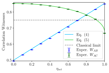
Figure 3: Experimental correlation witnesses (dots) as a function of the strength parameter that we set using Bob’s HWP. We also show the behavior predicted by Eqs. (4) and (5) (solid lines). We can see that there is region in which both witnesses are above the classical limit $\left(\frac{3}{4}\text{, dashed line}\right)$.

Figure 3 compares the individual witnesses with the expected values of Eqs. (4) and (5). We clearly see that we could sample the very interesting region in which both $W_{AB}$ and $W_{AC}$ are nonclassical.

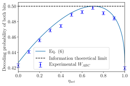
Figure 4: Probability of correctly decoding both of Alice’s bits when Bob and Charlie agree to target different bits.

Figure 4 confirms the validity of Eq. (6) and shows that if Bob and Charlie cooperate to decode the entire input sequence, they cannot succeed with probability better than $\frac{1}{2}$. However, this scheme does allow them to saturate the upper bound for a specific measurement strength.

Figure 5: Lower and upper bounds on the strength parameter, obtained by applying relations (7) and (8) to the experimental correlation witnesses.

Finally, we evaluated the self-testing capabilities of the protocol, computing upper and lower bounds on $\eta$ from the experimental $W_{AB}$ and $W_{AC}$ using Eqs. (7) and (8). Figure 5 plots them as a function of $\eta_{set}$. The tightness of the bounds is another proof that our setup achieved the optimal conditions C1-C3.

V DISCUSSION

Our experiment confirms the relations presented by MTB and proves that it is possible for two decoders in a QRAC to share higher success probabilities than admitted by classical physics. The quantum weak measurement is the key to this, as it allows reducing the disturbance on the state observed by the first decoder so that it can be used again by the second. This is a new situation in which weak measurements prove to be useful and to be able to overcome the limitations of axiomatic projective measurements.

A crucial point of this protocol is that it offers a different way to self-test quantum devices with limited assumptions: Observing the optimal values of $W_{AB}$ and $W_{AC}$ pinpoints (up to unitary transformations) Alice’s state preparation and Bob and Charlie’s measurements. Even without optimality, some properties of Bob’s measurements can be bounded. This is important for the characterization of setups that implement qubit measurements and require accurate strength setting or exploit incompatibility. We have also shown that the concept of sequential QRACs can provide a security bound for a SDI-QKD scenario. Additionally, in a communication scenario in which Bob and Charlie cooperate to decode the entirety of Alice’s string, there is one value of strength that can reach the performance limit imposed by information theory.

It would also be interesting to study robust self-testing relations for MTB’s scheme that can bound other properties of the quantum devices in suboptimal conditions. If needed, other assumptions could be added, e.g., perfect knowledge of Alice’s preparations could help characterize Bob and Charlie’s operations in a measurement-device-independent scenario.

Finally, extensions of Bob’s MZI scheme that allow full polarization measurements should be explored, considering also an implementation in integrated optics where polarizing directional couplers and polarization rotators are now feasible and could provide better accuracy than free-space discrete components Corrielli et al. (2014); Gao et al. (2015); Sarmiento-Merenguel et al. (2015); Pitsios et al. (2017).

APPENDIX A EXTENSION OF THE PROTOCOL TO MORE RECEIVERS

The protocol can be extended to any number of receivers if they all use weak measurements like Bob. However, we show here that this strategy does not allow more than two receivers two achieve correlation witnesses higher than $\frac{3}{4}$ together. Suppose the first receiver (Bob) uses strength parameter $\eta_{1}$, then,

$$W_{AB}(\eta_{1}) =\frac{1}{8}\sum_{x,y}\operatorname{tr}(\varrho_{x}M_{x_{y}|y})$$ (10)

$$=\frac{1}{2}+\frac{\sqrt{2}}{4}\eta_{1},$$

where $\varrho_{x}=\frac{1}{2}\left[\mathbb{1}+(-1)^{x_{0}}\frac{\sigma_{X}}{\sqrt{2}}+(-1)^{x_{1}}\frac{\sigma_{Z}}{\sqrt{2}}\right]$ is the state prepared by Alice and $M_{b|y}$ are the operators,

$$M_{0|0} =\frac{1}{2}(\mathbb{1}+\eta_{1}\sigma_{X}),$$ (11)

$$M_{1|0} =\frac{1}{2}(\mathbb{1}-\eta_{1}\sigma_{X}),$$

$$M_{0|1} =\frac{1}{2}(\mathbb{1}+\eta_{1}\sigma_{Z}),$$

$$M_{1|1} =\frac{1}{2}(\mathbb{1}-\eta_{1}\sigma_{Z}).$$

Note that $\{M_{0|0},M_{1|0}\}$ and $\{M_{0|1},M_{1|1}\}$ are two two-outcome POVMs, indeed, $\sum_{b}M_{b|y}=\mathbb{1},\ \forall y$. Moreover $\sum_{b}(-1)^{b}M_{b|0}=\eta_{1}\sigma_{X}$ and $\sum_{b}(-1)^{b}M_{b|1}=\eta_{1}\sigma_{Z}$, which is why these POVMs correspond to weak measurements of $\sigma_{X}$ and $\sigma_{Z}$, respectively. To each $M_{b|y}$ corresponds a Kraus operator $K_{b|y}$ such that $K_{b|y}^{\dagger}K_{b|y}=M_{b|y}$:

$$K_{0|0} =\frac{1}{2}\left[(\cos\mu_{1}+\sin\mu_{1})\mathbb{1}+(\cos\mu_{1}+\sin\mu_{1})\sigma_{X}\right],$$ (12)

$$K_{1|0} =\frac{1}{2}\left[(\cos\mu_{1}+\sin\mu_{1})\mathbb{1}-(\cos\mu_{1}+\sin\mu_{1})\sigma_{X}\right],$$

$$K_{0|1} =\frac{1}{2}\left[(\cos\mu_{1}+\sin\mu_{1})\mathbb{1}+(\cos\mu_{1}+\sin\mu_{1})\sigma_{Z}\right],$$

$$K_{1|1} =\frac{1}{2}\left[(\cos\mu_{1}+\sin\mu_{1})\mathbb{1}-(\cos\mu_{1}+\sin\mu_{1})\sigma_{Z}\right],$$

where $\mu_{1}=\frac{1}{2}\arccos(\eta_{1})$.

The second receiver (Charlie) ignores Bob’s measurement choice $y$ and outcome $b$, therefore, his correlation witness must be calculated from the postmeasurement state averaged over $y$ and $b$,

$$\varrho_{x}^{B} =\frac{1}{2}\sum_{y,b}K_{b|y}\varrho_{x}K_{b|y}^{\dagger}$$ (13)

$$=\frac{1}{2}\left[\mathbb{1}+\frac{1+\sqrt{1-\eta_{1}^{2}}}{2}\cdot\frac{(-1)^{x_{0}}\sigma_{X}+(-1)^{x_{1}}\sigma_{Z}}{\sqrt{2}}\right].$$

This expression is remarkably similar to the initial state $\varrho_{x}$ but contains factor $\frac{1+\sqrt{1-\eta_{1}^{2}}}{2}$ that shortens the Bloch vector of the state. Supposing that Charlie also performs weak measurements with strength parameter $\eta_{2}$, his correlation witness is:

$$W_{AC}(\eta_{1},\eta_{2}) =\frac{1}{8}\sum_{x,z}\operatorname{tr}(\varrho_{x}^{B}M_{x_{z}|z})$$ (14)

$$=\frac{1}{2}+\frac{\sqrt{2}}{4}\eta_{2}\frac{1+\sqrt{1-\eta_{1}^{2}}}{2},$$

which coincides with Eq. (5) for $\eta_{2}=1$.

This can continue for any number of receivers and the witness for the $n$th one is as follows:

$$W_{AR_{n}}(\eta_{1}\ldots\eta_{n})=\frac{1}{2}+\frac{\sqrt{2}}{4}\eta_{n}\prod_{i=1}^{n-1}\frac{1+\sqrt{1-\eta_{i}^{2}}}{2}.$$ (15)

This is an increasing function of $\eta_{n}$ but a decreasing one of $\eta_{i},\ \forall i<n$. It can be seen as a generalization of Eq. (15) of Ref. Mohan et al. (2019) and is similar to Eq. (24) of Ref. Mal et al. (2016) (for the case of $n=3$), which was obtained in the context of Bell inequality violations.

We can see from Eq. (10) that $W_{AB}>\frac{3}{4}$ for $\eta_{1}=\frac{1}{\sqrt{2}}+\epsilon_{1},\ \forall\epsilon_{1}>0$. Plugging this value into Eq. (14) shows that $W_{AC}>\frac{3}{4}$ for $\eta_{2}=2(\sqrt{2}-1)+\epsilon_{2},\ \forall\epsilon_{2}>(6\sqrt{2}-8)\epsilon_{1}+O(\epsilon_{1}^{2})$. A third receiver would then find

$$W_{AR_{3}}\left[\frac{1}{\sqrt{2}}+\epsilon_{1},2(\sqrt{2}-1)+\epsilon_{2},\eta_{3}\right]$$ (16)

$$\leq W_{AR_{3}}\left[\frac{1}{\sqrt{2}},2(\sqrt{2}-1),1\right]$$

$$= \frac{1}{2}+\frac{(\sqrt{2}+1)(1+\sqrt{8\sqrt{2}-11})}{16}\approx 0.735<\frac{3}{4},$$

where the first inequality is justified by the above monotonicity relations for Eq. (15). This means that if Bob and Charlie use measurements strong enough to overcome the classical bound, a third receiver cannot do so, even with maximal strength.

APPENDIX B FULL MEASUREMENTS WITH THE MACH-ZEHNDER INTERFEROMETER

The apparatus made up of a MZI and a HWP that Bob uses to perform the weak polarization measurements can only implement one Kraus operator at a time. As described in Sec. III, it is possible to switch from one to another by rotating HWPs before and after the MZI. However, there are many ways to change the scheme to make a full measurement possible without moving optical components. One is the replacement of PBDs with polarizing beam splitters which would make both exits available. A more detailed description of this proposal is in Ref. Foletto et al. (2019). The feasibility of bringing this idea to integrated optics should be explored, because direct translations of PBSs and wave plates exist Corrielli et al. (2014); Pitsios et al. (2017) and could allow better accuracy in a much more compact setup. However, if implemented with discrete optical table components, this scheme has the disadvantage that PBS-based MZIs are difficult to align. A more practical idea is the use of large PBDs that offer three exits, two of which would correspond to the other measurement outcome. They would still need to be recombined with further PBDs, which, if identical to the ones in the MZI, would not ruin the optical coherence. The beams could then reach Charlie, who could implement a full measurement using a PBS and two detectors for each input beam. HWPs would need to be rotated only to select the measurement basis. Figure 6 depicts this idea.

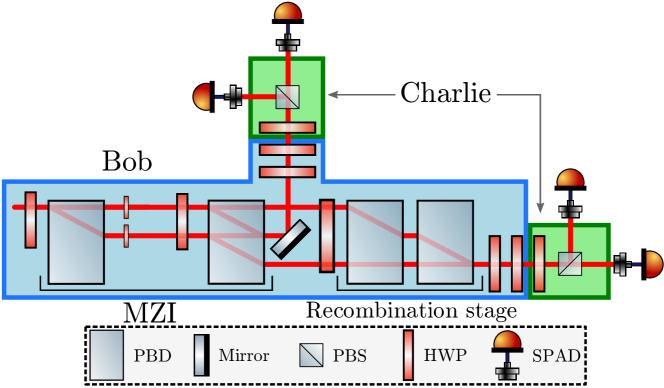
Figure 6: A possible scheme that extends the MZI used in the experiment to perform a full measurement. Charlie also performs a full measurement by placing detectors at both exits of his PBS.

Note that, with this scheme, Charlie would know Bob’s outcome by observing which detector clicks. If this information cannot be simply ignored and must be physically erased, one can imagine to further recombine Bob’s exit beams using a (nonpolarizing) beam splitter and delay lines before reaching a single PBS in Charlie’s setup.

APPENDIX C MORE DETAILS ON THE EXPERIMENT

Table 1 reports the angles of HWP_AB and HWP_BC that correspond to each setting of Alice’s preparation ($x_{0},x_{1}$), Bob’s measurement basis ($y$), Bob’s outcome ($b$), Charlie’s measurement basis ($z$), and Charlie’s outcome ($c$). As stated in the main text, HWP_H and HWP_V are fixed at angles 0 and $\pi/4$, respectively, whereas HWP_COM changes only with the measurement strength $\eta$, and its angle is $\theta=\frac{\pi-\arccos(\eta)}{4}$. A description of a very similar setup is also present in Ref. Foletto et al. (2019) with the difference that HWP_H and HWP_V are at angles $-\pi/8$ and $\pi/8$, respectively, and $\theta=\pi/8-\arccos(\eta)/4$. Indeed, the MZI works in the same way for any angle $\alpha$ of HWP_V as long as HWP_H is at angle $\alpha-\pi/4$ and HWP_COM is at $\theta=\alpha-\arccos(\eta)/4$. The coincident counts observed in the exposure time of 2 s for each configuration are also included in Table 1.

Table 1: HWP angles and coincident counts for each configuration of $x_{0},x_{1},y,b,z,\text{and }c$.

Settings						Angles (rad)		Coincident counts in 2 s. $\eta_{set}=\ldots$
$x_{0}$	$x_{1}$	$y$	$b$	$z$	$c$	HWPAB	HWPBC	$0$	$0.1$	$0.2$	$0.3$	$0.4$	$0.5$	$0.6$	$0.7$	$0.8$	$0.9$	$1$
0	0	0	0	0	0	$\pi/16$	$\pi/4$	2864	4709	5062	5313	5797	5379	5779	6437	6278	6517	6618
0	0	0	0	0	1	$\pi/16$	$\pi/2$	450	624	502	461	356	274	219	138	98	36	1
0	0	0	0	1	0	$\pi/16$	$\pi/8$	2840	4298	4461	4472	4363	4277	4209	4249	4137	3874	3396
0	0	0	0	1	1	$\pi/16$	$3\pi/8$	529	986	1200	1400	1561	1638	1978	2145	2483	2627	3521
0	0	0	1	0	0	$5\pi/16$	0	2988	3736	3402	2885	2298	1810	1486	1036	685	332	8
0	0	0	1	0	1	$5\pi/16$	$\pi/4$	425	784	792	863	861	801	927	954	1039	1021	1096
0	0	0	1	1	0	$5\pi/16$	$-\pi/8$	2944	4000	3798	3643	3373	2925	2422	2111	1709	1258	511
0	0	0	1	1	1	$5\pi/16$	$\pi/8$	598	657	432	353	177	118	44	16	18	101	563
0	0	1	0	0	0	$-\pi/16$	$3\pi/8$	2852	4476	4325	4556	4647	3964	4233	4026	4317	3797	3423
0	0	1	0	0	1	$-\pi/16$	$5\pi/8$	432	846	948	1172	1354	1491	1714	1872	2319	2459	3331
0	0	1	0	1	0	$-\pi/16$	$\pi/4$	2799	4492	4704	5124	5454	5270	5664	5809	6278	6565	6454
0	0	1	0	1	1	$-\pi/16$	$\pi/2$	570	716	688	533	434	354	314	209	149	82	1
0	0	1	1	0	0	$3\pi/16$	$\pi/8$	2970	4161	3992	3534	3447	2407	2543	2135	1931	1458	632
0	0	1	1	0	1	$3\pi/16$	$3\pi/8$	475	563	370	241	132	47	21	6	40	124	627
0	0	1	1	1	0	$3\pi/16$	0	2967	3849	3494	2881	2520	1984	1657	1132	816	358	3
0	0	1	1	1	1	$3\pi/16$	$\pi/4$	565	857	907	991	1035	1024	1058	1087	1218	1169	1227
0	1	0	0	0	0	$-\pi/16$	$\pi/4$	2757	4524	5024	5048	5342	5312	5971	6066	6399	6337	6672
0	1	0	0	0	1	$-\pi/16$	$\pi/2$	554	693	627	548	442	400	293	206	134	71	1
0	1	0	0	1	0	$-\pi/16$	$\pi/8$	540	886	1127	1258	1451	1338	1990	2062	2415	2703	3462
0	1	0	0	1	1	$-\pi/16$	$3\pi/8$	3006	4363	4543	4409	4451	3995	4320	4021	4062	3832	3522
0	1	0	1	0	0	$3\pi/16$	0	2999	3960	3516	2957	2426	1949	1654	1113	746	403	9
0	1	0	1	0	1	$3\pi/16$	$\pi/4$	561	885	972	962	1047	939	1162	1068	1205	1242	1248
0	1	0	1	1	0	$3\pi/16$	$-\pi/8$	456	547	402	281	169	82	23	7	20	129	701
0	1	0	1	1	1	$3\pi/16$	$\pi/8$	2981	4118	4014	3712	3373	2819	2725	2168	1952	1419	575
0	1	1	0	0	0	$-3\pi/16$	$3\pi/8$	2889	3920	3767	3441	3080	2788	2441	2015	1761	1300	513
0	1	1	0	0	1	$-3\pi/16$	$5\pi/8$	558	677	483	339	198	92	42	10	11	91	617
0	1	1	0	1	0	$-3\pi/16$	$\pi/4$	415	692	803	861	899	896	984	980	992	967	1151
0	1	1	0	1	1	$-3\pi/16$	$\pi/2$	2996	3923	3428	2983	2594	1868	1485	1122	723	339	10
0	1	1	1	0	0	$\pi/16$	$\pi/8$	2782	4381	4514	4463	4530	4358	4474	4188	4445	3852	3493
0	1	1	1	0	1	$\pi/16$	$3\pi/8$	575	946	1152	1370	1568	1664	1984	2234	2556	2754	3472
0	1	1	1	1	0	$\pi/16$	0	584	712	625	514	526	390	326	223	168	103	4
0	1	1	1	1	1	$\pi/16$	$\pi/4$	2875	4625	5018	5150	5543	5709	6184	6094	6379	6315	6570
1	0	0	0	0	0	$-5\pi/16$	$\pi/4$	540	854	930	953	1043	1008	1058	1140	1170	1159	1174
1	0	0	0	0	1	$-5\pi/16$	$\pi/2$	2920	3788	3365	2771	2268	1794	1416	1124	685	343	10
1	0	0	0	1	0	$-5\pi/16$	$\pi/8$	2827	4005	3724	3382	3210	2822	2602	2215	1810	1474	598
1	0	0	0	1	1	$-5\pi/16$	$3\pi/8$	443	528	346	242	151	54	16	7	53	147	652
1	0	0	1	0	0	$-\pi/16$	0	443	580	467	374	352	266	188	150	73	23	6
1	0	0	1	0	1	$-\pi/16$	$\pi/4$	2757	4601	4685	5179	5466	5458	5724	5854	6204	6432	6628
1	0	0	1	1	0	$-\pi/16$	$-\pi/8$	2766	4380	4347	4296	4365	4190	4357	4141	3959	3767	3128
1	0	0	1	1	1	$-\pi/16$	$\pi/8$	376	829	1007	1175	1370	1542	1723	1889	2290	2532	3253
1	0	1	0	0	0	$-7\pi/16$	$3\pi/8$	576	994	1153	1290	1504	1729	1860	2180	2546	2725	3414
1	0	1	0	0	1	$-7\pi/16$	$5\pi/8$	2872	4271	4389	4500	4339	4071	4244	4275	4031	4108	3212
1	0	1	0	1	0	$-7\pi/16$	$\pi/4$	2979	4670	4999	5214	5531	5557	6258	6090	6263	6660	6219
1	0	1	0	1	1	$-7\pi/16$	$\pi/2$	423	571	498	480	392	270	236	152	97	46	5
1	0	1	1	0	0	$-3\pi/16$	$\pi/8$	520	551	412	283	150	94	25	1	33	114	586
1	0	1	1	0	1	$-3\pi/16$	$3\pi/8$	2914	4136	3730	3380	2996	2664	2379	1995	1757	1296	523
1	0	1	1	1	0	$-3\pi/16$	0	2997	3692	3306	2869	2304	1843	1542	1030	669	293	13
1	0	1	1	1	1	$-3\pi/16$	$\pi/4$	383	686	706	816	816	887	945	961	1040	1043	970
1	1	0	0	0	0	$-3\pi/16$	$\pi/4$	415	691	744	762	838	860	950	1013	977	1059	1043
1	1	0	0	0	1	$-3\pi/16$	$\pi/2$	2975	3948	3352	2930	2434	1904	1535	1066	755	353	8
1	1	0	0	1	0	$-3\pi/16$	$\pi/8$	506	562	406	246	165	92	28	2	30	119	555
1	1	0	0	1	1	$-3\pi/16$	$3\pi/8$	2859	3977	3695	3384	2984	2687	2509	2011	1765	1392	515
1	1	0	1	0	0	$\pi/16$	0	551	776	649	599	430	402	281	268	171	82	6
1	1	0	1	0	1	$\pi/16$	$\pi/4$	2916	4722	5020	5356	5233	5407	5946	6202	6538	6627	6289
1	1	0	1	1	0	$\pi/16$	$-\pi/8$	523	935	992	1230	1421	1563	1901	1947	2379	2728	3400
1	1	0	1	1	1	$\pi/16$	$\pi/8$	2904	4386	4334	4475	4119	4218	4205	3970	3940	3914	2964
1	1	1	0	0	0	$-5\pi/16$	$3\pi/8$	462	479	386	228	146	64	15	7	36	119	637
1	1	1	0	0	1	$-5\pi/16$	$5\pi/8$	2942	4123	3801	3568	3064	2703	2678	2145	1817	1458	590
1	1	1	0	1	0	$-5\pi/16$	$\pi/4$	542	837	879	986	937	1034	1055	1002	1139	1114	1225
1	1	1	0	1	1	$-5\pi/16$	$\pi/2$	2844	3816	3398	2632	2203	1872	1467	1012	731	317	8
1	1	1	1	0	0	$-\pi/16$	$\pi/8$	497	910	1149	1300	1466	1675	1874	2055	2370	2581	3239
1	1	1	1	0	1	$-\pi/16$	$3\pi/8$	2969	4372	4605	4466	3927	4339	4399	4043	3961	3899	3235
1	1	1	1	1	0	$-\pi/16$	0	460	588	466	428	283	238	217	131	77	30	8
1	1	1	1	1	1	$-\pi/16$	$\pi/4$	2710	4428	4619	5019	4935	5534	5571	5918	6186	6298	6435

References

- Wiesner (1983) S. Wiesner, Conjugate coding, ACM SIGACT News 15, 78 (1983).
- Ambainis et al. (1999) A. Ambainis, A. Nayak, A. Ta-Shma, and U. Vazirani, Dense quantum coding and a lower bound for 1-way quantum automata, in Proceedings of the Thirty-First Annual ACM Symposium on Theory of Computing - STOC ’99, Atlanta, GA, 1999 (ACM, New York, 1999), pp. 376–383.
- Hayashi et al. (2006) M. Hayashi, K. Iwama, H. Nishimura, R. Raymond, and S. Yamashita, (4,1)-Quantum random access coding does not exist—one qubit is not enough to recover one of four bits, New J. of Phys. 8, 129 (2006).
- Iwama et al. (2007) K. Iwama, H. Nishimura, R. Raymond, and S. Yamashita, Unbounded-Error One-Way Classical and Quantum Communication Complexity, in Automata, Languages and Programming (Springer, Berlin/Heidelberg, 2007), pp. 110–121.
- Nayak (1999) A. Nayak, Optimal Lower Bounds for Quantum Automata and Random Access Codes, in Proceedings of the 40th Annual Symposium on Foundations of Computer Science, FOCS ’99, New York City, NY, 1999, (IEEE Computer Society, Washington DC, 1999), p. 369.
- Casaccino et al. (2008) A. Casaccino, E. F. Galvão, and S. Severini, Extrema of discrete Wigner functions and applications, Phys. Rev. A 78, 022310 (2008) .
- Tavakoli et al. (2015) A. Tavakoli, A. Hameedi, B. Marques, and M. Bourennane, Quantum Random Access Codes Using Single -Level Systems, Phys. Rev. Lett. 114, 170502 (2015) .
- Liabøtrø (2017) O. Liabøtrø, Improved classical and quantum random access codes, Phys. Rev. A 95, 052315 (2017).
- Ben-Aroya et al. (2008) A. Ben-Aroya, O. Regev, and R. de Wolf, A Hypercontractive Inequality for Matrix-Valued Functions with Applications to Quantum Computing and LDCs, in 2008 49th Annual IEEE Symposium on Foundations of Computer Science, Philadelphia, PA, 2008 (IEEE, Piscataway, NJ, 2008), pp. 477–486.
- Klauck (2001) H. Klauck, Lower bounds for quantum communication complexity, in Proceedings 42nd IEEE Symposium on Foundations of Computer Science, Newport Beach, CA, 2001 (IEEE, Piscataway, NJ, 2001) pp. 288–297.
- Hayashi et al. (2007) M. Hayashi, K. Iwama, H. Nishimura, R. Raymond, and S. Yamashita, Quantum Network Coding, in STACS 2007, edited by W. Thomas and P. Weil (Springer, Berlin/Heidelberg, 2007), pp. 610–621.
- Kerenidis and de Wolf (2004) I. Kerenidis and R. de Wolf, Exponential lower bound for 2-query locally decodable codes via a quantum argument, J. of Comput. and Syst. Sci. 69, 395 (2004) .
- Wehner et al. (2008) S. Wehner, M. Christandl, and A. C. Doherty, Lower bound on the dimension of a quantum system given measured data, Phys. Rev. A 78, 062112 (2008).
- Tavakoli et al. (2018) A. Tavakoli, J. Kaniewski, T. Vértesi, D. Rosset, and N. Brunner, Self-testing quantum states and measurements in the prepare-and-measure scenario, Phys. Rev. A 98, 062307 (2018) .
- Farkas and Kaniewski (2019) M. Farkas and J. Kaniewski, Self-testing mutually unbiased bases in the prepare-and-measure scenario, Phys. Rev. A 99, 032316 (2019).
- Li et al. (2012) H.-W. Li, M. Pawłowski, Z.-Q. Yin, G.-C. Guo, and Z.-F. Han, Semi-device-independent randomness certification using quantum random access codes, Phys. Rev. A 85, 052308 (2012).
- Lunghi et al. (2015) T. Lunghi, J. B. Brask, C. C. W. Lim, Q. Lavigne, J. Bowles, A. Martin, H. Zbinden, and N. Brunner, Self-Testing Quantum Random Number Generator, Phys. Rev. Lett. 114, 150501 (2015) .
- Li et al. (2015) D.-D. Li, Q.-Y. Wen, Y.-K. Wang, Y.-Q. Zhou, and F. Gao, Security of Semi-Device-Independent Random Number Expansion Protocols, Sci. Rep. 5, 15543 (2015).
- Pawłowski and Brunner (2011) M. Pawłowski and N. Brunner, Semi-device-independent security of one-way quantum key distribution, Phys. Rev. A 84, 010302(R) (2011) .
- Chaturvedi et al. (2018) A. Chaturvedi, M. Ray, R. Veynar, and M. Pawłowski, On the security of semi-device-independent QKD protocols, Quantum Inf. Process. 17, 131 (2018).
- Aharonov et al. (1988) Y. Aharonov, D. Z. Albert, and L. Vaidman, How the result of a measurement of a component of the spin of a spin- 1/2 particle can turn out to be 100, Phys. Rev. Lett. 60, 1351 (1988).
- Mitchison et al. (2007) G. Mitchison, R. Jozsa, and S. Popescu, Sequential weak measurement, Phys. Rev. A 76, 062105 (2007) .
- Schiavon et al. (2017) M. Schiavon, L. Calderaro, M. Pittaluga, G. Vallone, and P. Villoresi, Three-observer Bell inequality violation on a two-qubit entangled state, Quantum Sci. and Technol. 2, 015010 (2017) .
- Li et al. (2018) H.-W. Li, Y.-S. Zhang, X.-B. An, Z.-F. Han, and G.-C. Guo, Three-observer classical dimension witness violation with weak measurement, Commun. Phys. 1, 10 (2018).
- An et al. (2018) X.-B. An, H.-W. Li, Z.-Q. Yin, M.-J. Hu, W. Huang, B.-J. Xu, S. Wang, W. Chen, G.-C. Guo, and Z.-F. Han, Experimental three-party quantum random number generator based on dimension witness violation and weak measurement, Opt. Lett. 43, 3437 (2018).
- Chen et al. (2019) J.-S. Chen, M.-J. Hu, X.-M. Hu, B.-H. Liu, Y.-F. Huang, C.-F. Li, C.-G. Guo, and Y.-S. Zhang, Experimental realization of sequential weak measurements of non-commuting Pauli observables, Opt. Express 27, 6089 (2019) .
- Foletto et al. (2019) G. Foletto, L. Calderaro, A. Tavakoli, M. Schiavon, F. Picciariello, A. Cabello, P. Villoresi, and G. Vallone, Experimental Demonstration of Sustained Entanglement and Nonlocality After Sequential Measurements, Phys. Rev. Appl. 13, 044008 (2020) .
- Mohan et al. (2019) K. Mohan, A. Tavakoli, and N. Brunner, Sequential random access codes and self-testing of quantum measurement instruments, New J. of Phys. 21, 083034 (2019) .
- Mal et al. (2016) S. Mal, A. Majumdar, and D. Home, Sharing of Nonlocality of a Single Member of an Entangled Pair of Qubits Is Not Possible by More than Two Unbiased Observers on the Other Wing, Mathematics 4, 48 (2016) .
- Anwer et al. (2020) H. Anwer, S. Muhammad, W. Cherifi, N. Miklin, A. Tavakoli, and M. Bourennane, Experimental Characterization of Unsharp Qubit Observables and Sequential Measurement Incompatibility via Quantum Random Access Codes, Phys. Rev. Lett. 125, 080403 (2020) .
- Calderaro et al. (2018) L. Calderaro, G. Foletto, D. Dequal, P. Villoresi, and G. Vallone, Direct Reconstruction of the Quantum Density Matrix by Strong Measurements, Phys. Rev. Lett. 121, 230501 (2018) .
- Corrielli et al. (2014) G. Corrielli, A. Crespi, R. Geremia, R. Ramponi, L. Sansoni, A. Santinelli, P. Mataloni, F. Sciarrino, and R. Osellame, Rotated waveplates in integrated waveguide optics, Nat. Commun. 5, 4249 (2014).
- Gao et al. (2015) L. Gao, Y. Huo, K. Zang, S. Paik, Y. Chen, J. S. Harris, and Z. Zhou, On-chip plasmonic waveguide optical waveplate, Sci. Rep. 5, 15794 (2015).
- Sarmiento-Merenguel et al. (2015) J. D. Sarmiento-Merenguel, R. Halir, X. Le Roux, C. Alonso-Ramos, L. Vivien, P. Cheben, E. Durán-Valdeiglesias, I. Molina-Fernández, D. Marris-Morini, D.-X. Xu, J. H. Schmid, S. Janz, and A. Ortega-Moñux, Demonstration of integrated polarization control with a 40 dB range in extinction ratio, Optica 2, 1019 (2015).
- Pitsios et al. (2017) I. Pitsios, F. Samara, G. Corrielli, A. Crespi, and R. Osellame, Geometrically-controlled polarization processing in femtosecond-laser-written photonic circuits, Sci. Rep. 7, 11342 (2017) .