Analytical probabilistic modeling of dose-volume histograms

Abstract

Purpose: Radiotherapy, especially with charged particles, is sensitive to executional and preparational uncertainties that propagate to uncertainty in dose and plan quality indicators, e. g., dose-volume histograms. Current approaches to quantify and mitigate such uncertainties rely on explicitly computed error scenarios and are thus subject to statistical uncertainty and limitations regarding the underlying uncertainty model. Here we present an alternative, analytical method to approximate moments, in particular expectation value and (co)variance, of the probability distribution of DVH-points, and evaluate its accuracy on patient data.
Methods: We use Analytical Probabilistic Modeling (APM) to derive moments of the probability distribution over individual DVH-points based on the probability distribution over dose. By using the computed moments to parameterize distinct probability distributions over DVH-points (here normal or beta distributions), not only the moments but also percentiles, i. e., $\alpha$-DVHs, are computed. The model is subsequently evaluated on three patient cases (intracranial, paraspinal, prostate) in 30- and single-fraction scenarios by assuming the dose to follow a multivariate normal distribution, whose moments are computed in closed-form with APM. The results are compared to a benchmark based on discrete random sampling.
Results: The evaluation of the new probabilistic model on the three patient cases against a sampling benchmark proves its correctness under perfect assumptions as well as good agreement in realistic conditions. More precisely, ca. $90\text{\,}\mathrm{\char 37\relax}$ of all computed expected DVH-points and their standard deviations agree within $1\text{\,}\mathrm{\char 37\relax}$ volume with their empirical counterpart from sampling computations, for both fractionated and single fraction treatments. When computing $\alpha$-DVHs, the assumption of a beta distribution achieved better agreement with empirical percentiles than the assumption of a normal distribution: While in both cases probabilities locally showed large deviations (up to $\pm 0.2$), the respective $\alpha$-DVHs for $\alpha=\{0.05,0.5,0.95\}$ only showed small deviations in respective volume (up to $\pm 5\text{\,}\mathrm{\char 37\relax}$ volume for a normal distribution, and up to $2\text{\,}\mathrm{\char 37\relax}$ for a beta distribution). A previously published model from literature, which was included for comparison, exhibited substantially larger deviations.
Conclusions: With APM we could derive a mathematically exact description of moments of probability distributions over DVH-points given a probability distribution over dose. The model generalizes previous attempts and performs well for both choices of probability distributions, i. e., normal or beta distributions, over DVH-points.

1 Introduction

Recent years have shown an increased interest in adequate, patient-specific uncertainty quantification and mitigation for radiotherapy treatment planning both academically and clinically [[, see, e. g.,]and references therein]Unkelbach2018,Fredriksson2012. This development is, on the one hand, driven by emerging irradiation with particles and their characteristic sensitivity to uncertainties [3, 4]. On the other hand, it is facilitated by fast-growing computational capabilities that enable the computation of multiple dose scenarios with acceptable overhead.

Error dose scenarios are either computed as (1) worst case estimates, i. e., extreme realizations of the input uncertainty model which are used for robust optimization [[, as performed and evaluated within]]Pflugfelder2008,Lowe2016,Lowe2017,Fredriksson2011,Fredriksson2016,Casiraghi2013a,Liu2012, or (2) random samples from the probability distribution parameterizing the input uncertainty model [12, 13, 14, 15, 16, 17] for stochastic approaches. An explicit derivation of probabilistic models remains the exception [18, 19, 20, 21, 22].

Consequently, the analysis of plan uncertainty is based on the derived worst-case dose distributions or “error bar”-distributions with their respective histograms [11, 23, 6, 7], or statistical moments [24, 13, 21, 18, 22] as well as percentiles [14, 15, 17], according to the very optimization method used in the overall planning workflow. This use of empirical uncertainty estimates, however, exhibits limitations, in particular concerning statistical accuracy and the required recomputations during optimization due to the changing pencil-beam weights. Further, they conceal the inherent mathematical transformation from the input probability space (e. g. set-up and range uncertainties) to the probability distribution over dose and the respective plan quality indicator (QI). This aggravates their use in retrospective analyses and puts restrictions on the choice of optimization method and objectives, because the sampling pipeline cannot be inverted and/or efficiently differentiated.

Approaches which rigorously propagate the uncertainty may overcome these limitations. Since they are able to provide analytical objectives, constraints, and derivatives, they can introduce new mathematical simplifications and improve computational efficiency by exploiting the analytical formulation for both uncertainty quantification and mitigation with probabilistic optimization approaches [18, 22]. Because such approaches are not susceptible to statistical errors and the “curse of dimensionality” in scenario-based approaches, they deliver stable and reproducible results also for complex uncertainty models. However, derivation of such models is not trivial: Even if a model for dose probability is available, it still needs to be propagated to the derived plan indicators by hand. Other approaches overcome this step by re-sampling based on the derived dose uncertainty model [21, 20].

For DVH-points, analytical computation of moments of the probability distribution, given a probability distribution over the dose, has been attempted before [25, 26, 27]. However, [25, 26] only provide a model for the expected value of DVH-points with an upper bound on the DVHs’ standard deviation. Further, only simplified uncertainty models for the underlying dose distribution were assumed: while different shapes of the distributions were evaluated, correlations between voxels were not modeled, even though correlations having crucial impact on the higher moments of the depending probability distribution.

To derive a full model including correlations, this work will consequently not build on previous attempts, but provide a fresh start to a general methodology to compute the $\nu$-th moments of the probability distribution over DVH-points. The goal is to derive a generally applicable model for DVH-probabilities allowing arbitrary assumptions on the probability distribution over the dose distribution.

To do so, first a closed-form description for the moments of the probability distribution of DVH-points is derived. Then, these moments parameterize a probability distribution over the respective DVH-point. To evaluate our approach, three patient cases are investigated with statistical reference computations (using a large number of random dose samples from the probability distribution over set-up and range errors in fractionated and non-fractionated treatments). Along the lines of our validation campaign, we illustrate the shortcomings of previous work and highlight where wide approximations regarding the correlation models as exercised by [27] render meaningful quantification of DVH-probabilities impossible.

2 Materials & Methods

2.1 DVHs under uncertainty

2.1.1 Nominal computation

DVHs are cumulative histograms over the spatial dose distribution in a volume of interest (VOI) $v$, here expressed as vector $\boldsymbol{d}\in\mathbb{R}_{+}^{V}$ with number of voxels $V$. Hence, for any given dose parameter $\hat{d}$, a DVH-point $\mathrm{DVH}(\hat{d};\boldsymbol{d})\in[0,1]$ equals the fraction of the volume that receives at least dose $\hat{d}$. It can be expressed as averaged Heaviside steps

$$\mathrm{DVH}(\hat{d};\boldsymbol{d})=\frac{1}{V}\sum_{i\in v}\Theta(d_{i}-\hat{d})\,,$$ (1)

meaning that only voxels $i$ with $d_{i}\geq\hat{d}$ contribute to the sum which is normalized by the total voxel count $V$ in $v$ and thus yielding a fractional volume. Note that (without loss of generality) we assumed that all voxels have similar volume.

2.1.2 Uncertainty analysis of DVHs

Uncertainty analysis of DVHs is mostly performed on an empirical basis through computation of error dose scenarios [[, among others]]Park2013,Wahl2018,Kraan2013,Perko2016,Gordon2009,Gordon2010,Moore2009,Mescher2017,Unkelbach2009,Lowe2016,Lomax2008,Fredriksson2012. This enables the computation of a DVH for each dose scenario (which can be either a worst-case scenario or a random sample), from which then worst-case estimates, empirical statistical moments as well as quantiles of the probability distribution over DVH-points are derived.

For the purpose of this work, three forms of “statistical” DVHs will be of importance. First, uncertainty of a DVH can be evaluated through the statistical moments of each DVH-point, for example the expected/mean DVH and its standard deviation, which can be empirically determined from $n_{s}$ random dose samples $\boldsymbol{d}_{s}$ as

$$\overline{\mathrm{DVH}}(\hat{d}) =\frac{1}{n_{s}}\sum_{s=1}^{n_{s}}\mathrm{DVH}(\hat{d};\boldsymbol{d}_{s})$$ (2)

$$\sigma_{\mathrm{DVH}(\hat{d})} =\sqrt{\frac{1}{n_{s}-1}\sum_{s=1}^{n_{s}}\left[\mathrm{DVH}(\hat{d};\boldsymbol{d}_{s})-\overline{\mathrm{DVH}}(\hat{d})\right]^{2}}\,.$$ (3)

Secondly we discuss “$\alpha$-DVHs”, which can be compactly expressed as

$$\alpha\text{-\acs{DVH}}(\hat{d};\boldsymbol{d},\alpha)=v_{\alpha}\Leftrightarrow P(\mathrm{DVH}(\hat{d};\boldsymbol{d})\leq v_{\alpha})=\alpha$$ (4)

where $v_{\alpha}$ is the volume covered with a probability $P(\mathrm{DVH}(\hat{d})\geq v_{\alpha})=\alpha$. Thus $\alpha$-DVHs can be used to give percentiles of the probability distribution of each DVH-point and, together with the corresponding (1-$\alpha$)-DVH, the respective confidence intervals. $\alpha$-DVHs may be computed with the empirical marginal quantile functions for the respective DVH-points. Alternatively, $\alpha$-DVHs are equal to iso-probability curves on the respective dose-volume coverage map (DVCM) as proposed by [14]. Such a DVCM assigns a probability of coverage of each possible volume fraction for any dose threshold $\hat{d}$ and can be defined as

$$\mathrm{DVCM}(\hat{d},v;\boldsymbol{d})=P(\mathrm{DVH}(\hat{d};\boldsymbol{d})\leq v)=F_{\mathrm{DVH}(\hat{d},\boldsymbol{d})}(v)\,,$$ (5)

where $F_{\mathrm{DVH}(\hat{d},\boldsymbol{d})}(v)$ is the cumulative distribution function (CDF) of the probability distribution over the respective DVH-point. Equation 5 can then be directly inserted into Equation 4 such that the respective $\alpha$-DVH is now the iso-curve at $\mathrm{DVCM}=\alpha$.

Note that such $\alpha$-DVHs or DVCMs do not yield confidences or probabilities for the full DVH but only over single DVH-points (i. e., they represent marginal quantiles and CDFs), and hence do not generally represent naturally occuring DVH-scenarios.

2.2 Moments of the probability distribution over dose-volume histograms

2.2.1 Analytical integration

If the probability distribution over the dose $\boldsymbol{d}$ has the multivariate CDF $F_{\boldsymbol{d}}$, the $\nu$-th moment of the probability distribution of a transformation $I(\boldsymbol{d})$ can be computed via integration

$$\mathbb{E}\left[I(\boldsymbol{d})^{\nu}\right] =\int_{\mathbb{R}^{V}}I(\boldsymbol{\tilde{d}})^{\nu}\mathrm{d}F_{\boldsymbol{d}}(\boldsymbol{\tilde{d}})$$ (6a)

$$=\int_{\mathbb{R}^{V}}I(\boldsymbol{\tilde{d}})^{\nu}f_{\boldsymbol{d}}(\boldsymbol{\tilde{d}})\mathrm{d}\boldsymbol{\tilde{d}}\,.$$ (6b)

Moments of the probability distribution over a DVH may thus be explicitly calculated by solving Equation 6 for $I(\boldsymbol{d})=\mathrm{DVH}(\hat{d};\boldsymbol{d})$. For the first non-central moment, this yields

$$\mathbb{E}\left[\mathrm{DVH}(\hat{d};\boldsymbol{d})\right] =\int_{\mathbb{R}^{V}}\frac{1}{V}\sum_{i\in v}\Theta(\tilde{d}_{i}-\hat{d})f_{\boldsymbol{d}}(\boldsymbol{\tilde{d}})\mathrm{d}\boldsymbol{\tilde{d}}$$ (7a)

$$=\frac{1}{V}\sum_{i}\int_{-\infty}^{\infty}\Theta(\tilde{d}_{i}-\hat{d})f_{d_{i}}(\tilde{d}_{i})\mathrm{d}\tilde{d}_{i}$$ (7b)

$$=\frac{1}{V}\sum_{i}\int_{\hat{d}}^{\infty}f_{d_{i}}(\tilde{d}_{i})\mathrm{d}\tilde{d}_{i}$$ (7c)

$$=\frac{1}{V}\sum_{i}\left[1-F_{d_{i}}(\hat{d})\right]\,.$$ (7d)

Similar steps lead to the mixed non-central moment $\mathbb{E}\left[\mathrm{DVH}(\hat{d}_{p};\boldsymbol{d})\mathrm{DVH}(\hat{d}_{q};\boldsymbol{d})\right]$:

$$\mathbb{E}\left[\mathrm{DVH}(\hat{d}_{p};\boldsymbol{d})\mathrm{DVH}(\hat{d}_{q};\boldsymbol{d})\right] =\int_{\mathbb{R}^{V}}\frac{1}{V^{2}}\sum_{il\in v}\Theta(\tilde{d}_{i}-\hat{d}_{p})\Theta(\tilde{d}_{l}-\hat{d}_{q})f_{\boldsymbol{d}}(\hat{d})\mathrm{d}\boldsymbol{\tilde{d}}$$ (8a)

$$=\frac{1}{V^{2}}\sum_{il\in v}\int_{\mathbb{R}^{2}}\Theta(\tilde{d}_{i}-\hat{d}_{p})\Theta(\tilde{d}_{l}-\hat{d}_{q})f_{\boldsymbol{d}_{i;l}}(\boldsymbol{\tilde{d}}_{i;l})\mathrm{d}\tilde{\boldsymbol{d}_{i;l}}$$ (8b)

$$=\frac{1}{V^{2}}\sum_{il\in v}\int\limits_{\hat{d}_{p}}^{\infty}\int\limits_{\hat{d}_{q}}^{\infty}f_{\boldsymbol{d}_{i;l}}(\boldsymbol{\tilde{d}}_{i;l})\mathrm{d}\tilde{d}_{l}\mathrm{d}\tilde{d}_{i}\,.$$ (8c)

For the second non-central moment with $p=q$, i. e., $\mathbb{E}\left[\mathrm{DVH}(\hat{d}_{p};\boldsymbol{d})^{2}\right]$, Equation 8c can be expressed with the marginal bivariate cumulative distribution function $F_{\boldsymbol{d}_{i;l}}$ as

$$\mathbb{E}\left[\mathrm{DVH}(\hat{d};\boldsymbol{d})^{2}\right]=\frac{1}{V^{2}}\sum_{il\in v}\left[1-F_{\boldsymbol{d}_{i;l}}\left(\hat{d}\boldsymbol{1}_{2}\right)\right]\,,$$ (9)

where $\boldsymbol{1}_{2}=(1,1)^{T}$.

Together Equations 7, 8c and 9 then give the (co)variance of DVH-points at $\hat{d}_{p}$ and $\hat{d}_{q}$ using $\operatorname{Cov}\left[x,y\right]=\mathbb{E}\left[xy\right]-\mathbb{E}\left[x\right]\mathbb{E}\left[y\right]$, i. e.,

$$\operatorname{Cov}\left[\mathrm{DVH}(\hat{d}_{p};\boldsymbol{d}),\mathrm{DVH}(\hat{d}_{q};\boldsymbol{d})\right]\\ =\mathbb{E}\left[\mathrm{DVH}(\hat{d}_{p};\boldsymbol{d})\mathrm{DVH}(\hat{d}_{q};\boldsymbol{d})\right]-\mathbb{E}\left[\mathrm{DVH}(\hat{d}_{p};\boldsymbol{d})\right]\mathbb{E}\left[\mathrm{DVH}(\hat{d}_{q};\boldsymbol{d})\right]$$ (10)

which, in case of the variance of a DVH-point at $\hat{d}$, consequently reduces to

$$\operatorname{Var}\left[\mathrm{DVH}(\hat{d};\boldsymbol{d})\right]=\mathbb{E}\left[\mathrm{DVH}(\hat{d};\boldsymbol{d})^{2}\right]-\mathbb{E}\left[\mathrm{DVH}(\hat{d};\boldsymbol{d})\right]^{2}\,.$$ (11)

Hence, for each point of a DVH for a VOI $v$, Equations 7 to 11 allow explicit computation of the expected value and variance of a DVH as well as the covariance between all DVH points, valid for any probability distribution over the dose $\boldsymbol{d}$ in $v$ as long as its univariate and bivariate marginal CDF can be evaluated.

While not explicitly evaluated in this work, similar steps can be taken to compute higher moments to more accurately parameterize the underlying probability distribution. This requires an expansion of the respective power of the sums of Heaviside steps with the multinomial theorem and evaluation of multivariate probabilities of higher dimensionality. We provide such a generalization in Appendix C.

2.2.2 Summary of previous work

A result similar to Equation 7 was already documented in literature[25], where it was obtained by interpreting the computation of the DVH according to Equation 1 as a sum of Bernoulli experiments: Each voxel $i$ falls into the current DVH bin at $\hat{d}$ with a probability $p_{i}=P(d_{i}>\hat{d})=1-F_{d_{i}}(\hat{d})$, where $F_{d_{i}}$ is the marginal CDF for $d_{i}$, and does not fall into the bin with a probability $1-p_{i}$. With the linearity of the expectation value one then can directly derive Equation 7d.

The result proved to be applicable with different families of assumed probability distributions (i. e., Gaussian, triangular and rectangular/uniform)[25, 26]. However, due to the simplified uncertainty model using constant relative standard deviation and no correlation between voxels, an exact computation of higher moments of a DVH-point’s probability distribution was not attempted.

2.3 Confidence bounds for DVH-points

2.3.1 Parameterization of the DVH probability distribution

Since Equations 7 to 11 provide expected value and covariance of any DVH-point, one could possibly directly parameterize the probability distribution over the full DVH with a multivariate normal distribution. This parameterization is, however, unphysical; since DVH-points represent the fraction of a volume, their values are confined to the interval $[0,1]$ in contrast to the infinite support of the multivariate normal distribution. Hence, the probability distribution of a DVH point might be more “physically” represented by a distribution supported only in the interval $[0,1]$, such as a beta distribution $\mathcal{B}(a,b)$ with shape parameters $a$ and $b$. The beta distribution is shortly characterized in Appendix A. However, lacking a generalized multivariate form [[, for recent approaches on constructing bivariate beta distributions see, e. g.,]]Olkin2015,Nadarajah2017, $\mathcal{B}(a,b)$ may only be used to parameterize the marginal distribution over a single DVH-point, not the full multivariate DVH.

Current approaches applying DVH confidences define these on a marginal by-point basis [17, 14, 15, 29]. Hence, quantifying probabilities over marginal DVH-points is in line with literature and enables comparability. Therefore, in this work, marginal probabilities will be evaluated, based on the (unphysical) parameterization with normal distributions as well as the more physical approach using a beta distribution whose shape parameters $a$ and $b$ are obtained from the respective DVH-point’s expectation value and variance with Equations 23 and 24.

Using either a normal or beta distribution, one can directly compute DVCMs according to Equation 5 or an $\alpha$-DVH using

$$\alpha\text{-DVH}(\hat{d};\boldsymbol{d},\alpha) =F^{-1}_{\mathrm{DVH}(\hat{d};\boldsymbol{d})}(\alpha)$$ (12)

$$=\begin{cases}\mathbb{E}\left[\mathrm{DVH}(\hat{d};\boldsymbol{d})\right]+\sqrt{2\operatorname{Var}\left[\mathrm{DVH}(\hat{d};\boldsymbol{d})\right]}\operatorname{erf}^{-1}(2\alpha-1)&\text{| normal}\\ I^{-1}_{\alpha}(a,b)&\text{| beta}\end{cases}\,,$$

where $\operatorname{erf}^{-1}$ denotes the inverse error function and $I^{-1}_{\alpha}$ represents the inverse of the regularized incomplete beta-function.

2.3.2 Summary of previous work

A subsequent work[27] to [*]Henriquez2008,Henriquez2008a already formulated an analyitcal calculation of $\alpha$-DVHs as defined in Equation 4. In summary, their model is based on the definition of a “binary random variable”[27]

$$T_{i}^{\alpha,\hat{d}}=\begin{cases}1&P(d_{i}\geq\hat{d})>1-\alpha\\ 0&P(d_{i}\geq\hat{d})\leq 1-\alpha\end{cases}$$ (13)

interpreted as “the volume receiving a dose greater than [$\hat{d}$] with a probability greater than $1-\alpha$”[27]. This interpretation then leads them to define $T_{i}^{\alpha,\hat{d}}=\Theta\left(1-\alpha-F_{d_{i}}(\hat{d})\right)$ which, in analogy to Equation 4, translates to

$$\alpha\text{-DVH}^{\text{HC}}(\hat{d};\boldsymbol{d},\alpha)=\frac{1}{V}\sum_{i\in v}T_{i}^{\alpha,\hat{d}}=\frac{1}{V}\sum_{i\in v}\Theta\left(1-\alpha-F_{d_{i}}(\hat{d})\right)\,.$$ (14)

Equation 14 substantially differs from our result in Equation 12. This may be attributed to disregarding correlation across voxels in their derivations or inconsistencies in the definition of $T_{i}^{\alpha,\hat{d}}$, which apparently does not describe a random variable per se, but rather includes the evaluation of a probability—in this case the probability $P(d_{i}-\hat{d})$ of uncertain dose $d_{i}$ exceeding $\hat{d}$—which is not a random but a fixed value obtained from the CDF over $d_{i}$. Since Equation 14 has only been tested with an assumed uncertainty model and not been benchmarked against sample statistics[27], we incorporate Equation 14 in our evaluations and discuss the Equation further in Section 4.

2.4 Dose Uncertainty Model

Evaluation of Equations 7, 11 and 10 or, in general, Equation 25 requires a model for the probability distribution over dose $\boldsymbol{d}$, such that its CDF can be evaluated. Note that empirical CDFs as well as analytical/parameterized CDFs can be used.

2.4.1 Gaussian model for the probability distribution over dose

For a first evaluation and validation of the new probabilistic computations, we assume

$$\boldsymbol{d}\sim\mathcal{N}(\boldsymbol{\mu},\Sigma)\,,$$ (15)

i. e., the dose follows a multivariate normal distribution with mean dose $\boldsymbol{\mu}$ and covariance $\Sigma$. This choice of probability distribution cannot represent the true underlying probability distribution: First, the multivariate normal is supported on the full multidimensional real space, while physical dose is bound to the positive orthant. And second, empirical evidence [[, e. g. ]]Park2013,Lowe2016 as well as heuristic considerations show that the respective distribution exhibits considerable skewness and is consequently not part of the symmetric Gaussian family. Alternatives to assumption (15) will be discussed in Section 4. As a first order approximation, however, Equation 15 is well suited to study the probabilistic DVH-model, because on the one hand, its univariate and bivariate probabilities can be calculated [32], which is sufficient to compute an expected DVH and its (co)variance. On the other hand, evaluation on patient cases with assumption (15) implicitly studies the impact of the inaccurate Gaussian dose model on the evaluation of VOI-based dose statistics like DVHs under uncertainty. Further, while for a single fraction treatment the non-Gaussian shape of the probability distribution over dose is to be expected, under multiple fractions a more Gaussian-like shape may form [[, for examples of voxel dose probability distributions see]]Park2013,Lowe2016.

2.4.2 Computation of dose uncertainty

The Gaussian dose model from Section 2.4.1 requires mean $\boldsymbol{\mu}$ and covariance $\Sigma$ for evaluation. E. g., these could be empirically estimated with sample mean and covariance of a set of discrete error scenarios.

Since the motivation of this work is to build a fully analytical model (which also facilitates future use in optimization), we rely on computation of $\boldsymbol{\mu}$ and $\Sigma$ through APM as introduced by [18]. In previous works we could already show that APM accurately models $\boldsymbol{\mu}$ and $\boldsymbol{\sigma}=\sqrt{\operatorname{diag}(\Sigma)}$ [33], and that efficient application to patient data—especially in the context of fractionation [22]—is possible. [34] further extended it to biological optimization by demonstrating APMs applicability to intensity-modulated carbon ion therapy planning.

APM acts as a probabilistic pencil-beam dose calculation algorithm inherently enabling computation of moments of the probability distribution over the resulting dose. More exact, APM represents the constituents of a pencil-beam algorithm as superpositions of Gaussian functions (including the integrated depth dose, i. e., the Bragg peak), enabling propagation of uncertainties through the dose calculation in closed-form via analytical integration [[, for a detailed explanation see]]Bangert2013.

The accuracy of this approximation of the pencil-beam algorithm can, in principle, be arbitrarily chosen by varying the number of Gaussian components, thus providing also a nominal dose calculation algorithm for inverse treatment planning that is similar in quality to common pencil-beam algorithms. As such, it is able to provide a dose influence matrix $D\in\mathbb{R}_{+}^{V\times B}$ with number of voxels $V$ and number of pencil-beams $B$ generating the dose $\boldsymbol{d}\in\mathbb{R}_{+}^{V}$ from the fluence vector $\boldsymbol{w}\in\mathbb{R}_{+}^{B}$ via the linear transformation

$$d_{i}=\sum_{j}D_{ij}w_{j}\,.$$ (16)

In Equation 16, $i$ indexes voxels in the patient while $j$ indexes pencil-beams.

Now, in addition to Equation 16, APM provides probabilistic analogs to Equation 16 for moments of the probability distribution over $\boldsymbol{d}$ by enabling element-wise computation of expectation value and (co)variance of elements of the dose influence matrix $D$. This allows to represent the expected value of dose $\mathbb{E}\left[\boldsymbol{d}\right]$ as a linear transformation

$$\mathbb{E}\left[d_{i}\right]=\sum_{j}\underbrace{\mathbb{E}\left[D_{ij}\right]}_{\mathcal{D}_{ij}}w_{j}=\sum_{j}\mathcal{D}_{ij}w_{j}$$ (17)

and the covariance in dose with a quadratic form

$$\operatorname{Cov}\left[d_{i},d_{l}\right]=\sum_{jm}\underbrace{\operatorname{Cov}\left[D_{ij},D_{lm}\right]}_{\mathcal{V}_{ijlm}}w_{j}w_{m}=\sum_{jm}\mathcal{V}_{ijlm}w_{j}w_{m}\,.$$ (18)

Hence, one can denote $\mathcal{D}\in\mathbb{R}_{+}^{V\times B}$ and $\mathcal{V}\in\mathbb{R}_{+}^{V\times B\times V\times B}$ as expected dose influence matrix and covariance influence tensor, respectively. While $\mathcal{V}$ is, in general, too large to be stored in memory, the element-wise computation with APM allows on-the-fly evaluation of dependent quantities, e. g. the variance or covariance of dose.

2.5 Validation and application of the model

The analytical probabilistic DVH-model will be evaluated on three patient cases, i. e., an intracranial, a paraspinal, and a prostate case. Parameters used for planning and uncertainty computations are laid out in Table 1. These cases were already evaluated in our previous works [33, 22, 34]. Furthermore, a detailed comparison of $\alpha$-DVHs and DVCMs is exercised to validate empirical percentiles against results from the respective quantile functions from Equation 4 and the previous works by [27].

2.5.1 Application on all cases using the fractionated treatment samples

For all three patient cases, empirical estimates $\overline{\mathrm{DVH}}$, $\bar{\sigma}^{2}_{\mathrm{DVH}}$ are obtained by computing $$100$\times$30$$ dose scenarios, i. e., $100$ sampled treatment scenarios with $30$ fraction each, based on a Gaussian uncertainty model using the assumed setup and range errors from Table 1 as respective standard deviation with zero mean [[, compare to the description of the APM uncertainty model in]]Bangert2013. Additionally, expected dose $\boldsymbol{\mu}$ and covariance $\Sigma$ within the respective VOIs was also computed with APM (see Section 2.4.2) for the same input uncertainty model, and then fed into the herein presented DVH-models (by assuming a multivariate normal distribution as described in Section 2.4). This enabled comparison of the sample statistics to a fully analytical method and serves as proof-of-concept of the derived model.

2.5.2 Full validation on the intracranial case with $5000$ samples

As the intracranial case is the smallest one with lowest computational overhead, we further computed $5000$ realizations of single-fraction treatments. These will be used to nearly eliminate statistical inaccuracy for benchmarking APM.

To further validate the analytical computation itself excluding inherent mismatch of modeled and real probability distribution over dose, the analytically computed $\boldsymbol{\mu}$ and $\Sigma$ are additionally used to create $5000$ new dose samples under the assumption that dose actually follows a multivariate normal distribution, i. e., their samples are drawn from the distribution $\mathcal{N}(\boldsymbol{\mu},\Sigma)$. From these samples, a second statistical estimate of the DVH is obtained. This can be used to validate if the analytical computation is actually correct under the multivariate normal assumption from Equation 15. Further, DVCMs and $\alpha$-DVHs are computed under the assumption of marginally normally distributed DVH-points and marginally beta distributed DVH-points. These are compared to the respective statistical estimates from the $5000$ scenario samples.

3 Results

We evaluated the described methodology on three patient cases – an intracranial, paraspinal, and prostate patient. Information about the datasets, treatment plans and the assumed input uncertainty model can be found in Table 1.

3.1 Proof of work – computation on patient data

Figure 1 compares sample mean and standard deviation of DVHs to the respective analytical computations with Equations 7 to 11 for treatments with $30$ fractions.

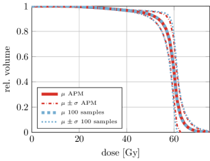
(a) paraspinal, CTV

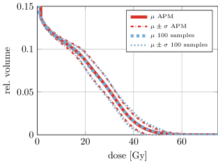
(b) paraspinal, spinal cord

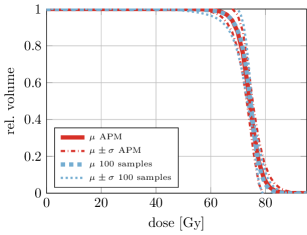
(c) prostate, boost

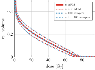
(d) prostate, rectum

(e) intracranial, CTV

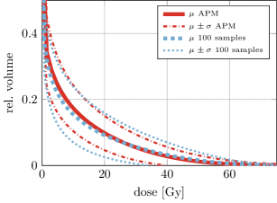
(f) intracranial, brainstem

Figure 1: Analytically computed expectation value and standard deviation of DVHs of a target volume and OAR for each of the three patient cases, compared to the respective sample mean and standard deviation. For the sampling benchmark, $100$ treatments were simulated by multivariate normal sampling using the systematic errors from Table 1 as standard deviation, while for each treatment taking $30$ fraction samples based on the random component.

For the prostate case, the sampled and analytically computed mean DVH and its standard deviation yield good agreement for both target and OAR. For the intracranial case, especially the curves illustrating standard deviation seem to exhibit larger differences. However, a closer look reveals that the differences originate from both discrepancies of the mean and the standard deviation estimates.

To better quantify the differences between the analytical computation and the sample reference, Figure 2 summarizes the absolute difference in relative volume for all patients grouped by (1) mean and standard deviation, (2) targets and OARs, and (3) 1 and 30 fraction treatments. Differences between analytical and sample computations are, in general, larger for targets than for OARs. For the OARs, the evaluation for multiple fractions shows an increase in accuracy. This does not seem to transfer to targets, where, although the number of points with minimal difference ($<$0.001$$) also increases, a stronger tail to higher differences is present. In general, more outliers, i. e., single DVH-points with large difference, can be observed when performing the calculations for a treatment in 30 fractions.

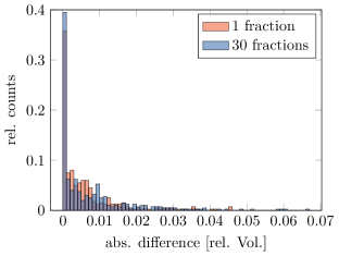
(a) mean, all targets

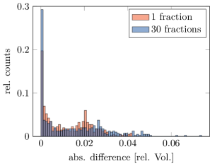
(b) standard deviation, all targets

(c) mean, all OARs

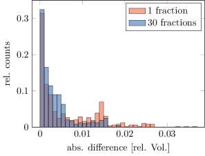
(d) standard deviation, all OARs

Figure 2: Histograms (bin width: $0.001$) of the absolute differences observed between the mean and standard deviation of all DVH-points computed analytically and via random sampling for all patients. (a,b) show the analysis for all evaluated targets in all patients, while (c,d) display it for all evaluated OARs.

3.2 Validation of model and analytical computations

3.2.1 Distribution of single DVH-points

Figure 3 shows normalized histograms of two DVH-points (one evaluated at $57\text{\,}\mathrm{Gy}$ for the target and one at $30\text{\,}\mathrm{Gy}$ for the brainstem of the intracranial case), comparing the samples from the dose scenarios and from the multivariate normal approximation. Their respective approximations with a normal distribution visualize differences between the respective moments of the DVH-point’s probability distribution: in the CTV, the re-sampled mean underestimates the DVH at $57\text{\,}\mathrm{Gy}$ by a volume fraction of $4\text{\,}\mathrm{\char 37\relax}$, whereas in the brainstem difference between the mean / expected values is negligible. The opposite holds true for the computed standard deviation.

(a) CTV

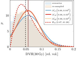
(b) brainstem

Figure 3: Probability distribution over DVH-points evaluated at $\hat{d}=$57\text{\,}\mathrm{Gy}$$ in the CTV (a) and at $30\text{\,}\mathrm{Gy}$ in the brainstem (b) of the intracranial case. The histograms show the distribution from the $5000$ dose scenarios and the $5000$ dose distributions re-sampled under assumption (15). $\mathcal{N}_{\mathcal{S}}$ represents a normal distribution parameterized from sample mean and variance from the $5000$ DVHs obtained from the scenario samples, $\mathcal{N}_{\mathcal{R}}$ has ben similarly computed from the re-sampled scenarios. $\mathcal{N}_{\mathcal{A}}$ parameterizes a normal distribution based on the analytical (APM) computation of DVH-point expectation and variance, and $\mathcal{B}_{\mathcal{A}}$ uses the same values to parameterize a beta distribution. The vertical lines indicate the respective expected/mean values, with the dashed black line giving the nominal value.

The analytically computed expectation value and variance of the respective DVH-points shows no significant difference to the statistical moments obtained from the re-sampled data. This is expected, since the analytical computations are mathematically exact and only negligible numerical inaccuracy is introduced when evaluating the univariate and bivariate normal CDF.

The Gaussian approximation is not bound to the volumetric interval $[0,1]$, and thus would assign non-zero probability to non-existing, e. g., negative, volume fractions. Figure 3 thus shows corresponding approximations with beta distributions, whose shape parameters are obtained from Equations 23 and 24 using analytically computed expectation and variance of the DVH-point. This leads to a physically more reasonable distribution which is further backed by the Q-Q plots comparing the quantiles of the normal and beta approximation to the empirical quantiles in Figure 4.

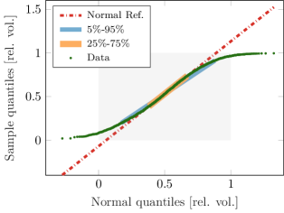
(a) CTV

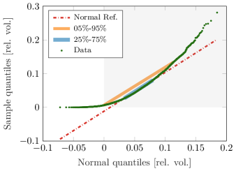
(b) brainstem

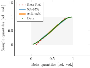
(c) CTV

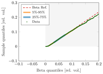
(d) brainstem

Figure 4: Quantile-quantile plots comparing empirical quantiles (y-axis) for the data (green) to quantiles from the hypothesized normal (a,b) and beta (c,d) distributions (x-axis) obtained from analytical moment computations (red). The thicker green and yellow lines span the $5\text{\,}\mathrm{\char 37\relax}95\text{\,}\mathrm{\char 37\relax}$ and $25\text{\,}\mathrm{\char 37\relax}75\text{\,}\mathrm{\char 37\relax}$ quantiles, respectively. In each plot the gray area additionally enclose “physically feasible” volumes in $[0,1]$. CTV and brainstem of the intracranial case are shown for the same DVH-points as in Figure 3. The data is based on the $5000$ dose scenario samples for a single fraction.

Figures 4(a) and 4(b) underline the problem of the infinite support of the normal distribution, i. e., unphysical quantiles exist in the theoretical normal model. This goes hand in hand with an especially pronounced disagreement between theoretical and empirical quantiles approaching the boundaries of the interval $[0,1]$, but also concerns possible skewness (compare Figures 4(b) and 3(b)) or excess kurtosis of the distribution (Figures 4(a) and 3(a)). These disagreements are reduced using a beta distribution. Especially the evaluated DVH-point in the brainstem in Figure 4(d) shows near perfect agreement with the empirical quantiles. For all four evaluations in Figure 4, however, near perfect agreement is achieved for “inner” quantiles, i. e., the first and third quartile.

3.2.2 Evaluation of cumulative probabilities

Next, we assess the accuracy of complete $\alpha$-DVHs by comparing $\alpha$-DVHs computed from the quantile functions of the respective probability distribution parameterized from the analytical computations with empirical quantiles over the full DVH. Furthermore we compare to the previous attempt of analytical computation of $\alpha$-DVHs [27] as laid out in Section 2.3.2.

Figure 5 shows the respective comparisons of analytically computed DVCMs to DVCMs obtained from sample statistics (compare Equation 5). The $\alpha$-DVHs in Figures 5(a) and 5(b) computed with Equation 14, i. e., the method from [27], show significant differences to the corresponding reference $\alpha$-DVHs from sampling.

(a) CTV, DVCM_S

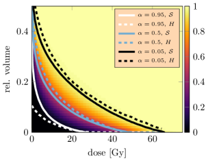
(b) brainstem, DVCM_S

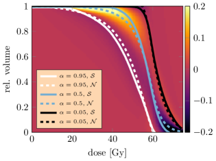
(c) CTV, DVCM_N – DVCM_S

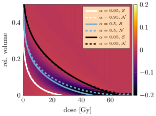
(d) brainstem, DVCM_N – DVCM_S

(e) CTV, DVCM_B – DVCM_S

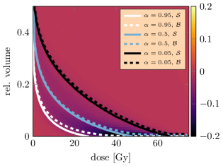
(f) brainstem, DVCM_B – DVCM_S

Figure 5: Evaluation of probabilities and $\alpha$-DVHs obtained through scenario sampling and analytical computations. (a) and (b) show empirical DVCMs (indexed with $\mathcal{S}$) obtained from the $5000$ dose scenarios, where the color indicates the local value of the CDF of the respective DVH-point. Corresponding $\alpha$-DVHs were derived, based on sampling ($\mathcal{S}$) and on [27] ($\mathcal{H}$). For (c) and (d) the difference of DVCM_N, a DVCM constructed from the normal parameterization, to DVCM_S has been evaluated with corresponding $\alpha$-DVHs obtained from the normal quantile function. (e,f) provide a similar analysis using DVCM_B and $\alpha$-DVHs ($\mathcal{B}$) with the beta parameterization.

In Figures 5(c) and 5(d), the probabilities within the empirical DVCMs show large differences when compared to DVCMs computed with the CDF from the Gaussian approximation, especially near full volume coverage and near zero volume coverage, where the approximated CDF exhibits differences of up to $\pm 0.2$. This is to be expected due to the infinite support of the normal distribution, and therefore the agreement is much better with the beta approximation in Figures 5(e) and 5(f) (overall the deviation is more than halved compared to the normal approximation). This transfers to the computation of $\alpha$-DVHs based on the quantile function of the beta distribution, similarly showing better agreement than with the assumption of normally distributed DVH-points. Overall, our explicit parametrization and evaluation of quantile functions of either normal or especially beta distributions outperforms the previously published method[27] (compare Section 2.3.2).

4 Discussion

The very core of this work is the description of an analytical model that can compute statistical moments of DVH-points for arbitrary probability distributions over the dose distribution. The only requirement is that the dose distribution follows/obeys a probability distribution function where the marginal CDFs can be evaluated. Hence, we provide a mathematically exact formulation of the moments which eliminates statistical uncertainty (in particular in combination with APM-based uncertainty quantification [18, 22]); if the probability distribution over dose is known, the respective moments can be exactly computed.

In our initial analysis, a multivariate normal distribution was assumed based on expected dose and its covariance obtained from a probabilistic dose calculation employing APM, which we compared to a sampling benchmark. Most of the analytically computed expected and standard deviations of the investigated DVHs lied within $\pm 1.5\text{\,}\mathrm{\char 37\relax}$ difference in volume from the sampling benchmark. Evaluating the same model for a larger number of fractions showed that especially for the OARs, more values cluster around the small differences.

Those differences between analytical model and sampling benchmark mainly stem from the assumed probability distribution over the dose distribution. It is clear that the multivariate normal assumption for dose uncertainty used throughout this work does not reflect every detail of reality perfectly. This is directly obvious because dose cannot be negative while the normal distribution has infinite support. But also deformations and anatomical variations, the non-linearity of dose deposition, and the so far not captured complexity of input uncertainty suggest that “real” dose uncertainty will most likely manifest as non-Gaussian probability distributions differing across heavily interdependent voxels. For parametrizing such models, an appropriate family of probability distributions that reasonably models variation in voxel doses would have to be selected for which correlations could then, for example, be modeled with copulas. While finding a suitable probabilistic model accurately describing dose distributions under uncertainty is beyond the scope of this work, our method would also be compatible with such advanced models, since it only requires that some form of multivariate CDF can be computed. This includes non-Gaussian analytical as well as empirical CDFs. In doing so our model has the advantage to preserve the mathematical connection between dose DVH-variation which would not be accessible when sampling DVH-scenarios themselves.

Despite the inaccuracy inherent to our choice of a multivariate normal distribution, it served as good initial proof of concept for the presented method. The multivariate normal parametrization allowed straightforward resampling of dose scenarios to demonstrate the exactness of the closed-form solution. The validation with results from sampled dose cubes and DVHs on the three patient cases showed that despite using this physically flawed model, we still obtain reasonable results, especially for the prostate and paraspinal case. The larger deviations in the intracranial case may be attributed to the smaller VOIs compared to the other two cases. The above discussed observation that fractionation seems to decrease the difference in most voxels might be attributed to a more Gaussian shaped probability distribution of dose uncertainty in the context of fractionation [[, as also indicated within]]Lowe2017.

Our model describes moments of the DVH-points’ probability distributions and not the probability distribution over the full DVHs. Therefore it is not directly possible to exactly compute confidences on actual realizations of the full DVH. It is, however, possible to use the computed moments to parameterize distributions over DVH points. In our evaluations based on expected DVH-points and their standard deviation, usage of normal distributions was a first obvious choice. To some extent it may be surprising that this yielded acceptable results within few volume percent difference to the sampling benchmark: The choice of a normal distribution (with infinite support) is in this case of a volume fraction, which can take only values in the interval $[0,1]$, similarly physically unreasonable as in the case of the dose distribution. A more plausible (concerning the support interval) parameterization was found using a beta distribution. However, both distributions do not represent a mathematically exact model. Interpreting the calculation of a DVH-point as a series of Bernoulli trials [[, similar to ]see Section 2.2.2]Henriquez2008, suggests parameterization with a Binomial distribution in the case of independently and identically distributed individual voxel doses. Still, assuming independence of voxels would not be realistic. More suitable correlated binomial models [35] make specific assumptions and are computationally demanding, rendering them not applicable for our purpose. Nevertheless, assuming a beta distribution (or even a normal distribution), which is parameterized by mean and standard deviation for the DVH-point, could facilitate uncertainty propagation through models that build on DVHs itself, e. g. in deriving biologically effective dose [36], or refining the statistical models for optimization purposes [19].

In comparison to the previous works[25, 26, 27], our methodology directly reproduced their model for the expectation value of DVH-points [25]. Our approach using integration directly generalizes to higher moments like covariance, while their model only yielded upper bounds on the variance because correlations between voxels were not explicitly included. Yet, despite the lack of an uncertainty model considering covariance in dose, they formulated confidence bounds, i. e., $\alpha$-DVHs [27]. Those were, however, in stark disagreement with the sampling benchmark (and thence our model). This may mainly be attributed to neglecting the contribution of (in)dependencies between voxels in the derivations. The difference of Equation 14 to a “true” confidence of dose over coverage of a volume fraction may be shown by the following gedankenexperiment: Let us assume all $V$ voxels in a VOI $v$ are independently normally distributed with a mean value of $\hat{d}$ and identical variances, and therefore exhibiting $F_{d_{i}}(\hat{d})=$0.5$$ in all voxels $i\in v$. In this setup, one can see that the median DVH-point at $\hat{d}$ takes the value $0.5$. Yet, plugging this into Equation 14 with again $\alpha=$0.5$$ yields $\alpha\text{-DVH}^{\text{HC}}(\hat{d})=\frac{1}{V}\cdot V\cdot\Theta(1-0.5-0.5)=1\neq$0.5$$ (depending on the definition of the Heaviside-step). Furthermore, in this case Equation 14 exhibits a sharp “step” around $\hat{d}$: For smaller doses $\hat{d}-\epsilon$, the argument of the step function in Equation 14 becomes negative and therefore resulting in $\alpha\text{-DVH}(\hat{d}-\epsilon)=1$, while for larger doses it becomes $\alpha\text{-DVH}(\hat{d}-\epsilon)=0$. For the assumed independently distributed model, however, a smooth decrease of the median DVH around $\hat{d}$ is expected, whereas the step would be correctly reproduced when assuming perfectly correlated voxels. Instead we suggest to interpret their result as the “fraction of voxels whose probability of exceeding $\hat{d}$ independently from each other is larger than $1-\alpha$”. Such a quantity, however, does not have a palpable clinical interpretation.

The applicability of a method that propagates uncertainty from dose to DVHs in terms of treatment planning might not be directly obvious. As discussed in Section 1, uncertainty quantification usually relies on sampled (stochastic approach) or selected (worst-case approach) dose scenarios, which can directly be used to obtain similar uncertainty information about the DVH. However, the analytical probabilistic method presented here provides a closed-form, continuous relationship between dose uncertainty and DVH-uncertainty, which can be useful in treatment planning.

For optimization purposes with probabilistic constraints, the method facilitates the use of continuous differentiable functions, which “fill the gap” between empirical samples, and could possibly enable exact definition of the “allowed” probability that certain clinical constraints are failing. There, using the parameterization of the probability distribution over a DVH-point, we now have functional access to the probability that a specific dose level is covered with a certain probability via the $\alpha$-DVH and its analytical dependence on mean and covariance of the dose (instead of nominal dose as for conventional non-probabilisitc objectives).[37, 38] Using this information for planning would extend widely used margin principles[39, 40], which are themselves defined based on demanding tumor coverage with a desired probability for a given dose level. Compared to common robust approaches where the worst case is dynamically found from a discrete pre-defined uncertainty subset in the input variables, an analytical confidence constraint based on $\alpha$-DVHs captures the full uncertainty space and allows for definition of the desired robustness on the relevant endpoint. For example, $90\text{\,}\mathrm{\char 37\relax}$ probability to cover a tumor with the $95\text{\,}\mathrm{\char 37\relax}$ of the prescribed dose could reproduce common margin assumptions also for anatomically complex cases where margins break down, while at the same time other probabilistic or nominal endpoints could be optimized. Since these objectives (or also constraint functions) continue to be functions of mean and covariance of dose, optimization would remain possible using conventional (quasi-)Newton optimizers. This, however, comes at the cost of deriving the arguably complex gradients (w.r.t. dose mean & covariance), which could be mitigated by using automatic differentiation [41], accompanied by a computationally challenging, yet “embarrassingly parallel” (co)variance computation.[37, 38] Further, the role of model inaccuracy in such a probabilistic optimization approach would need to be further investigated—[42], however, suggest that the assumption of normal distributions in probabilistic optimization still enables mitigation of dose uncertainties even if the “real” distribution differs substantially. A full analysis of computational performance and resulting dose distributions of such an optimization approach would exceed this manuscript and may be part of a future study.

Further, the probabilistic model only requires the dose’s probability distribution and is independent of the method used to obtain it. This allows its general application, e. g., in (retrospective) plan analyses or in combination with sampling-based stochastic optimization approaches. For plan analysis and comparison, the closed-form connection of dose and DVH-uncertainty could be used to observe how higher dose uncertainty (simulated by scaling covariance in desired voxels, for example) would impact the DVH and therefore target coverage. When relying on sample statistics for the dose instead of a probabilstic dose calculation, the parameterizations can be useful to extrapolate to areas not covered by samples. Additionally, the method could also be used in scenarios where computation of uncertainties statistically is no longer possible (e. g. when analysing an older cohort) based on assumptions over the dose probability distributions while still retaining the mathematical link between dose and DVH probabilities, which may be useful for machine learning applications investigating plan uncertainties.

And last but not least, the generral concept does not only apply to the computation of DVH points. As already indicated by [37], the concept may—given mathematical efforts—be extended to other plan quality metrics as mean dose or equivalent uniform dose (EUD), or distinct treatment planning objective and constraint functions.

5 Conclusion

We presented a method to calculate moments of the probability distribution over DVH-points given a known probability distribution over the dose distribution. The resulting analytical model corrects and generalizes previous attempts and can be readily combined with every method able to quantify a probability distribution over dose of either empirical or probabilistic nature.

We successfully benchmarked the model against excessive sampling (with and without fractionation), proving mathematical correctness and good agreement even with unrealistic but common assumptions for probability distributions within the computational pipeline. The methodology can serve as blueprint for future models on other QIs and can provide a generalizable framework for confidence-constrained probabilistic treatment plan optimization.

Appendix A Beta distribution

Suppose a random variable $X$ follows a beta distribution, i. e., $X\sim\mathcal{B}(a,b)$ with shape parameters $a$ and $b$.

Within the interval $x\in[0,1]$ (for $a>b>1$, $x\in(0,1)$ otherwise) its probability density function (PDF) $f_{X}(x)$ is given by

$$f_{X}(x)=\frac{1}{\mathrm{B}(a,b)}x^{a-1}(1-x)^{b-1}$$ (19)

where the normalization $\mathrm{B}(a,b)$ is the beta-function.

The CDF

$$F_{X}(x)=I_{x}(a,b)$$ (20)

requires evaluation of the regularized incomplete beta-function $I_{x}$.

Expectation and variance of $X$ are then given by

$$\mathbb{E}\left[X\right] =\frac{a}{a+b}\,,$$ (21)

$$\operatorname{Var}\left[X\right] =\frac{ab}{(a+b+1)(a+b)^{2}}=\frac{\mathbb{E}\left[X\right]^{2}b}{a^{2}+ab+a}\,.$$ (22)

The shape parameters $a$ and $b$ can be inferred from sample statistics, i. e., the sample mean $\bar{x}$ and the sample variance $\bar{\sigma}^{2}$, with the method of moments based on Equations 21 and 22 for $\bar{\sigma}^{2}<\bar{x}(1-\bar{x})$:

$$\hat{a} =\bar{x}\left(\frac{\bar{x}(1-\bar{x})}{\bar{\sigma}^{2}}-1\right)\,,$$ (23)

$$\hat{a} =(1-\bar{x})\left(\frac{\bar{x}(1-\bar{x})}{\bar{\sigma}^{2}}-1\right)=\bar{x}(1-\bar{x})\hat{a}\,.$$ (24)

Appendix B Patient Data Information

Table 1: Information on the three patient datasets used for evaluation (similar to [22]).

patient	intra-cranial	para-spinal	prostate
beam angles	$60\text{\,}\mathrm{\SIUnitSymbolDegree}120\text{\,}\mathrm{\SIUnitSymbolDegree}$	$135\text{\,}\mathrm{\SIUnitSymbolDegree}180\text{\,}\mathrm{\SIUnitSymbolDegree}225\text{\,}\mathrm{\SIUnitSymbolDegree}$	$90\text{\,}\mathrm{\SIUnitSymbolDegree}270\text{\,}\mathrm{\SIUnitSymbolDegree}$
prescribed dose	$60\text{\,}\mathrm{Gy}$	$60\text{\,}\mathrm{Gy}$	$70\text{\,}\mathrm{Gy}$ ($76\text{\,}\mathrm{Gy}$)
beamlet distance	$3\text{\,}\mathrm{mm}$	$4\text{\,}\mathrm{mm}$	$5\text{\,}\mathrm{mm}$
#beamlets	1705	13274	6803
resolution	$($1.2$\times$1.2$\times$3$)\,${\mathrm{mm}}^{3}$$	$($3$\times$3$\times$3$)\,${\mathrm{mm}}^{3}$$	$($2$\times$2$\times$3$)\,${\mathrm{mm}}^{3}$$
setup error [std. dev.]	$($1\text{\,}\mathrm{mm}$)^{\text{sys}}+($2\text{\,}\mathrm{mm}$)^{\text{rand}}$	$($1\text{\,}\mathrm{mm}$)^{\text{sys}}+($2\text{\,}\mathrm{mm}$)^{\text{rand}}$	$($1\text{\,}\mathrm{mm}$)^{\text{sys}}+($3\text{\,}\mathrm{mm}$)^{\text{rand}}$
range error [std. dev.]	$($3.5\text{\,}\mathrm{\char 37\relax}$)^{\text{sys}}+($1\text{\,}\mathrm{mm}$)^{\text{rand}}$	$($3.5\text{\,}\mathrm{\char 37\relax}$)^{\text{sys}}+($1\text{\,}\mathrm{mm}$)^{\text{rand}}$	$($3.5\text{\,}\mathrm{\char 37\relax}$)^{\text{sys}}+($1\text{\,}\mathrm{mm}$)^{\text{rand}}$

Appendix C Generalized model for the $\nu$-th moment of a probability distribution over a DVH-point

Using multi-index notation with the multi-index $\boldsymbol{\kappa}=\left(\kappa_{1},\kappa_{2},\ldots,\kappa_{V}\right)\in\mathbb{N}_{0}^{V}$ and by definition of a multi-indexed Heaviside step $\Theta^{\boldsymbol{\kappa}}(\boldsymbol{\tilde{d}}-\hat{d})=\prod_{i=1}^{n}\Theta(\tilde{d}_{i}-\hat{d})^{\kappa_{i}}$, one can provide a compact general formula to compute the $\nu$-th non-central moment of the probability distribution of a DVH-point, i. e.,

$$\mathbb{E}\left[\mathrm{DVH}(\hat{d};\boldsymbol{d})^{\nu}\right] =\int_{\mathbb{R}^{n}}\frac{1}{V^{\nu}}\sum_{|\boldsymbol{\kappa}|=\nu}\begin{pmatrix}\nu\\ \boldsymbol{\kappa}\end{pmatrix}\Theta^{\boldsymbol{\kappa}}(\boldsymbol{\tilde{d}}-\hat{d})f_{\boldsymbol{d}}(\boldsymbol{\tilde{d}})\mathrm{d}\boldsymbol{\tilde{d}}$$ (25)

$$=\frac{1}{V^{\nu}}\sum_{|\boldsymbol{\kappa}|=\nu}\begin{pmatrix}\nu\\ \boldsymbol{\kappa}\end{pmatrix}\left[1-F_{\boldsymbol{d}_{\kappa}}(\hat{d}\cdot\boldsymbol{1}_{\nu})\right]$$

where $F_{\boldsymbol{d}_{\kappa}}(\hat{d}\cdot\boldsymbol{1}_{\nu})$ corresponds to the evaluation of a $\nu$-variate marginal probability and $\boldsymbol{1}_{\nu}\in\mathbb{R}^{\nu}$ is a vector with each of the $\nu$ components equal to $1$. For example, in the case of $\nu=3$ and $V=4$, given an index combination $\boldsymbol{\kappa}=(2,0,1,0)$ (satisfying the sum condition $|\boldsymbol{\kappa}|=\nu=3$), the trivariate probability $F_{\boldsymbol{d}_{1;1;3}}((\hat{d},\hat{d},\hat{d})^{T})$ needs to be evaluated. Note that the possible “doubling” of an index (i. e., $\kappa_{i}>1$) can also be eliminated in the underlying integral using $\Theta(x)^{\kappa_{i}}=\Theta(x)$. This reduces the given example to an evaluation of a bivariate probability $F_{\boldsymbol{d}_{1;3}}((\hat{d},\hat{d})^{T})=F_{\boldsymbol{d}_{1;1;3}}((\hat{d},\hat{d},\hat{d})^{T})$.

References

- [1] Jan Unkelbach et al. “Robust radiotherapy planning” In Physics in Medicine and Biology 63.22 IOP Publishing, 2018, pp. 22TR02 DOI: 10.1088/1361-6560/aae659
- [2] Albin Fredriksson “A characterization of robust radiation therapy treatment planning methods—from expected value to worst case optimization” In Medical Physics 39.8 American Association of Physicists in Medicine, 2012, pp. 5169–5181 DOI: 10.1118/1.4737113
- [3] Antony John Lomax “Intensity modulated proton therapy and its sensitivity to treatment uncertainties 1: the potential effects of calculational uncertainties.” In Physics in Medicine and Biology 53.4, 2008, pp. 1027–1042 DOI: 10.1088/0031-9155/53/4/015
- [4] A J Lomax “Intensity modulated proton therapy and its sensitivity to treatment uncertainties 2: the potential effects of inter-fraction and inter-field motions” In Physics in Medicine and Biology 53.4, 2008, pp. 1043–1056 DOI: 10.1088/0031-9155/53/4/015
- [5] Daniel Pflugfelder, Jan Jakob Wilkens and Uwe Oelfke “Worst case optimization: a method to account for uncertainties in the optimization of intensity modulated proton therapy.” In Physics in Medicine and Biology 53.6 IOP Publishing, 2008, pp. 1689–700 DOI: 10.1088/0031-9155/53/6/013
- [6] Matthew Lowe et al. “Incorporating the effect of fractionation in the evaluation of proton plan robustness to setup errors” In Physics in Medicine and Biology 61.1 IOP Publishing, 2016, pp. 413–429 DOI: 10.1088/0031-9155/61/1/413
- [7] Matthew Lowe et al. “A robust optimisation approach accounting for the effect of fractionation on setup uncertainties” In Physics in Medicine and Biology 62.20 IOP Publishing, 2017, pp. 8178–8196 DOI: 10.1088/1361-6560/aa8c58
- [8] Albin Fredriksson, Anders Forsgren and Björn Hårdemark “Minimax optimization for handling range and setup uncertainties in proton therapy” In Medical Physics 38.3 American Association of Physicists in Medicine, 2011, pp. 1672–1684 DOI: 10.1118/1.3556559
- [9] Albin Fredriksson and Rasmus Bokrantz “The scenario-based generalization of radiation therapy margins” In Physics in Medicine and Biology 61.5 IOP Publishing, 2016, pp. 2067–2082 DOI: 10.1088/0031-9155/61/5/2067
- [10] M Casiraghi, F Albertini and Antony John Lomax “Advantages and limitations of the ’worst case scenario’ approach in IMPT treatment planning.” In Physics in Medicine and Biology 58.5 IOP Publishing, 2013, pp. 1323–1339 DOI: 10.1088/0031-9155/58/5/1323
- [11] Wei Liu, Xiaodong Zhang, Yupeng Li and Radhe Mohan “Robust optimization of intensity modulated proton therapy” In Medical Physics 39.2 American Association of Physicists in Medicine, 2012, pp. 1079–1091 DOI: 10.1118/1.3679340
- [12] Jan Unkelbach, Timothy C Y Chan and Thomas Bortfeld “Accounting for range uncertainties in the optimization of intensity modulated proton therapy.” In Physics in Medicine and Biology 52.10, 2007, pp. 2755–2773 DOI: 10.1088/0031-9155/52/10/009
- [13] Jan Unkelbach, Thomas Bortfeld, Benjamin C. Martin and Martin Soukup “Reducing the sensitivity of IMPT treatment plans to setup errors and range uncertainties via probabilistic treatment planning.” In Medical Physics 36.2009 American Association of Physicists in Medicine, 2009, pp. 149–163 DOI: 10.1118/1.3021139
- [14] J J Gordon and J V Siebers “Coverage-based treatment planning: optimizing the IMRT PTV to meet a CTV coverage criterion.” In Medical Physics 36.3, 2009, pp. 961–973 DOI: 10.1118/1.3075772
- [15] J J Gordon, N Sayah, E Weiss and J V Siebers “Coverage optimized planning: probabilistic treatment planning based on dose coverage histogram criteria.” In Medical Physics 37.2, 2010, pp. 550–563 DOI: 10.1118/1.3273063
- [16] Román Bohoslavsky, Marnix G Witte, Tomas M Janssen and Marcel Herk “Probabilistic objective functions for margin-less IMRT planning” In Physics in Medicine and Biology 58.11, 2013, pp. 3563–3580 DOI: 10.1088/0031-9155/58/11/3563
- [17] H Mescher, S Ulrich and M Bangert “Coverage-based constraints for IMRT optimization” In Physics in Medicine and Biology 62.18 IOP Publishing, 2017, pp. N460–N473 DOI: 10.1088/1361-6560/aa8132
- [18] Mark Bangert, Philipp Hennig and Uwe Oelfke “Analytical probabilistic modeling for radiation therapy treatment planning.” In Physics in Medicine and Biology 58.16, 2013, pp. 5401–5419 DOI: 10.1088/0031-9155/58/16/5401
- [19] B. Sobotta, M. Söhn and M. Alber “Robust optimization based upon statistical theory” In Medical Physics 37.8 American Association of Physicists in Medicine, 2010, pp. 4019–4028 DOI: 10.1118/1.3457333
- [20] B Sobotta, M Söhn and M Alber “Accelerated evaluation of the robustness of treatment plans against geometric uncertainties by Gaussian processes” In Physics in Medicine and Biology 57.23 IOP Publishing, 2012, pp. 8023–8039 DOI: 10.1088/0031-9155/57/23/8023
- [21] Zoltán Perkó et al. “Fast and accurate sensitivity analysis of IMPT treatment plans using Polynomial Chaos Expansion.” In Physics in Medicine and Biology 61.12 IOP Publishing, 2016, pp. 4646–4664 DOI: 10.1088/0031-9155/61/12/4646
- [22] Niklas Wahl, Philipp Hennig, Hans-Peter Wieser and Mark Bangert “Analytical incorporation of fractionation effects in probabilistic treatment planning for intensity-modulated proton therapy” In Medical Physics 45.4, 2018, pp. 1317–1328 DOI: 10.1002/mp.12775
- [23] S E McGowan, F Albertini, S J Thomas and A J Lomax “Defining robustness protocols: a method to include and evaluate robustness in clinical plans.” In Physics in Medicine and Biology 60.7 IOP Publishing, 2015, pp. 2671–2684 DOI: 10.1088/0031-9155/60/7/2671
- [24] Peter C. Park et al. “Statistical assessment of proton treatment plans under setup and range uncertainties” In International Journal of Radiation Oncology*Biology*Physics 86.5 Elsevier Inc., 2013, pp. 1007–1013 DOI: 10.1016/j.ijrobp.2013.04.009
- [25] Francisco Cutanda Henríquez and Silvia Vargas Castrillón “A Novel Method for the Evaluation of Uncertainty in Dose-Volume Histogram Computation” In International Journal of Radiation Oncology*Biology*Physics 70.4, 2008, pp. 1263–1271 DOI: 10.1016/j.ijrobp.2007.11.038
- [26] Francisco Cutanda Henríquez and Silvia Vargas Castrillón “The effect of the different uncertainty models in dose expected volume histogram computation” In Australasian Physical and Engineering Sciences in Medicine 31.3, 2008, pp. 196–202
- [27] Francisco Cutanda Henríquez and Silvia Vargas Castrillón “Confidence intervals in dose volume histogram computation” In Medical Physics 37.4, 2010, pp. 1545–1553 DOI: 10.1118/1.3355888
- [28] Aafke C. Kraan et al. “Dose uncertainties in IMPT for oropharyngeal cancer in the presence of anatomical, range, and setup errors” In International Journal of Radiation Oncology*Biology*Physics 87.5 Elsevier Inc., 2013, pp. 888–896 DOI: 10.1016/j.ijrobp.2013.09.014
- [29] Joseph A Moore, John J Gordon, Mitchell S Anscher and Jeffrey V Siebers “Comparisons of treatment optimization directly incorporating random patient setup uncertainty with a margin-based approach.” In Medical Physics 36.9, 2009, pp. 3880–3890 DOI: 10.1118/1.3176940
- [30] Ingram Olkin and Thomas A. Trikalinos “Constructions for a bivariate beta distribution” In Statistics & Probability Letters 96 North-Holland, 2015, pp. 54–60 DOI: 10.1016/j.spl.2014.09.013
- [31] Saralees Nadarajah, Shou Hsing Shih and Daya K. Nagar “A new bivariate beta distribution” In Statistics 51.2 Taylor & Francis, 2017, pp. 455–474 DOI: 10.1080/02331888.2016.1240681
- [32] Alan Genz “Numerical computation of rectangular bivariate and trivariate normal and t probabilities” In Statistics and Computing 14.3, 2004, pp. 251–260 DOI: 10.1023/B:STCO.0000035304.20635.31
- [33] Niklas Wahl, Philipp Hennig, Hans-Peter Wieser and Mark Bangert “Efficiency of analytical and sampling-based uncertainty propagation in intensity-modulated proton therapy” In Physics in Medicine and Biology 62.14, 2017, pp. 5790–5807 DOI: 10.1088/1361-6560/aa6ec5
- [34] Hans-Peter Wieser, Philipp Hennig, Niklas Wahl and Mark Bangert “Analytical probabilistic modeling of RBE-weighted dose for ion therapy” In Physics in Medicine and Biology 62.23 IOP Publishing, 2017, pp. 8959–8982 DOI: 10.1088/1361-6560/aa915d
- [35] M. Hisakado, K. Kitsukawa and S. Mori “Correlated Binomial Models and Correlation Structures” In Journal of Physics A: Mathematical and General 39.50, 2006, pp. 15365–15378 DOI: 10.1088/0305-4470/39/50/005
- [36] Thomas E. Wheldon, Charles Deehan, Elizabeth G. Wheldon and Ann Barrett “The linear-quadratic transformation of dose–volume histograms in fractionated radiotherapy” In Radiotherapy and Oncology 46.3, 1998, pp. 285–295 DOI: 10.1016/S0167-8140(97)00162-X
- [37] Niklas Wahl “Analytical Models for Probabilistic Inverse Treatment Planning in Intensity-modulated Proton Therapy”, 2018 DOI: 10.11588/heidok.00025127
- [38] Niklas Wahl, Philipp Hennig, Hans-Peter Wieser and Mark Bangert “Confidence constraints for probabilistic radiotherapy treatment planning” In 19th International Conference on the Use of Computers in Radiation Therapy (ICCR), 2019
- [39] Marcel Herk, Peter Remeijer, Coen Rasch and Joos V. Lebesque “The probability of correct target dosage: dose-population histograms for deriving treatment margins in radiotherapy” In International Journal of Radiation Oncology*Biology*Physics 47.4, 2000, pp. 1121–1135 URL: http://www.sciencedirect.com/science/article/pii/S0360301600005186
- [40] Marcel Herk “Errors and margins in radiotherapy” In Seminars in Radiation Oncology 14.1, 2004, pp. 52–64 DOI: 10.1053/j.semradonc.2003.10.003
- [41] Andreas Griewank and Andrea Walther “Evaluating Derivatives”, Other Titles in Applied Mathematics Society for Industrial and Applied Mathematics, 2008 DOI: 10.1137/1.9780898717761
- [42] Hans-Peter Wieser, Christian P. Karger, Niklas Wahl and Mark Bangert “Impact of Gaussian uncertainty assumptions on probabilistic optimization in particle therapy” In Physics in Medicine and Biology, 2020 DOI: 10.1088/1361-6560/ab8d77