Suppressing thermalisation and constructing weak solutions in truncated inviscid equations of hydrodynamics: Lessons from the Burgers equation

Abstract

Finite-dimensional, inviscid equations of hydrodynamics, obtained through a Fourier-Galerkin projection, thermalise with an energy equipartition. Hence, numerical solutions of such inviscid equations, which typically have to be Galerkin-truncated, show a behaviour at odds with the parent equation. An important consequence of this is an uncertainty in the measurement of the temporal evolution of the distance of the complex singularity from the real domain leading to a lack of a firm conjecture on the finite-time blow-up problem in the incompressible, three-dimensional Euler equation. We now propose, by using the one-dimensional Burgers equation as a testing ground, a novel numerical recipe, named tyger purging, to arrest the onset of thermalisation and hence recover the true dissipative solution. Our method, easily adapted for higher dimensions, provides a tool to not only tackle the celebrated blow-up problem but also to obtain weak and dissipative solutions—conjectured by Onsager and numerically elusive thus far—of the Euler equation.

Introduction:

Non-linear, partial differential equations of hydrodynamics, such as the inviscid the one-dimensional Burgers or the three-dimensional Euler equations, are often studied, numerically and theoretically, by projecting them on to a Fourier subspace with a finite number of modes bounded by a (large) wavenumber ${K_{\scriptscriptstyle\mathrm{G}}}$. This projection (defined precisely later), known as a Galerkin-projection, ensures that unlike the parent partial differential equation (PDE) which has an infinite number of degrees of freedom, the Galerkin-truncated equation is constrained to have only finitely many Fourier modes. Consequently, the resulting finite-dimensional, inviscid equations of hydrodynamics, such as the three-dimensional (3D) incompressible Euler equations or the one-dimensional (1D) Burgers equation, conserve both energy and phase-space, leading to solutions which thermalise in a finite-time. These solutions are thus completely different from the solutions of the actual partial differential equation, from which they derive, with infinite degrees of freedom Hopf (1950); Lee (1952).

In recent years however, this area has received renewed interest Ray (2015)—spanning studies in turbulence Frisch et al. (2012); Lanotte et al. (2015, 2016); Buzzicotti et al. (2016a, b); Ray (2018), bottlenecks and hyperviscosity Frisch et al. (2008, 2013); Banerjee and Ray (2014) to problems of cross-correlators in condensed matter physics Kumar et al. (2019)—beginning with the work of Majda and Timofeyev Majda and Timofeyev (2000) on the thermalisation of the Galerkin-truncated, 1D inviscid Burgers equation. Subsequently, Cichowlas, et al. Cichowlas et al. (2005), through state-of-the-art direct numerical simulations (DNSs) showed the existence of similar thermalised states in the Galerkin-truncated 3D incompressible Euler equation (see, also, Ref. Krstulovic and Étienne Brachet (2008)). However the precise mechanism by which solutions thermalise was discovered later by Ray, et al. Ray et al. (2011) who showed that thermalisation was triggered through a resonant-wave-like interaction leading to localised structures christened tygers (see, also, Refs. Pereira et al. (2013); Clark Di Leoni et al. (2018); Venkataraman and Ray (2017)).

Understanding Galerkin-truncated systems assumes a special importance when numerically studying inviscid equations for the problem of finite-time blow-up of the incompressible Euler equation (under suitable conditions). A way to conjecture for or against a finite-time singularity is to numerically solve the Euler equation and measure the width of the analyticity strip $\delta$ Sulem et al. (1983), i.e., the distance to the real domain of the nearest complex singularity. By assuming analyticity, at least up to a hypothetical time of blow-up $t_{*}$, this procedure reduces to measuring the Fourier modes of the velocity field $\hat{u}_{k}\sim\exp{[-\delta(t)k]}$ (ignoring vectors for convenience), for large wavenumbers $k$, and thence, $\delta$ as a function of time $t$. Therefore, a numerically compelling proof for finite-time blow-up is to show $\delta(t)\to 0$ in a finite time.

Simple as it sounds, such an approach unfortunately runs into a severe problem in its implementation. To solve such equations on the computer, one has to make them finite-dimensional through a Galerkin truncation. Solutions to such truncated equations thermalise, beginning at small scales (or large wavenumbers $k$) in a finite time. Hence, asymptotically at large wavenumbers the Fourier modes of the velocity field grow as a power law $\hat{u}_{k}\sim k^{d-1}$ (energy equipartition), where $d$ is the spatial dimension, and not fall-off exponentially from which the width of the analyticity strip can be extracted. Hence, the measurement of $\delta(t)$ becomes unreliable soon enough to prevent us from making a reasonable conjecture of if and when $\delta(t)$ might vanish Bustamante and Brachet (2012). Therefore, in order to have a more reliable measurement of $\delta(t)$ for times long enough to conjecture on whether there is a finite-time blow-up of, e.g., the 3D, incompressible, Euler equation, it is vital to have a (numerical) prescription—without resorting to viscous damping—which prevents the solutions from thermalising.

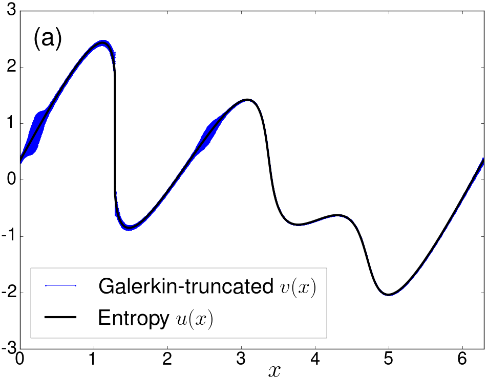
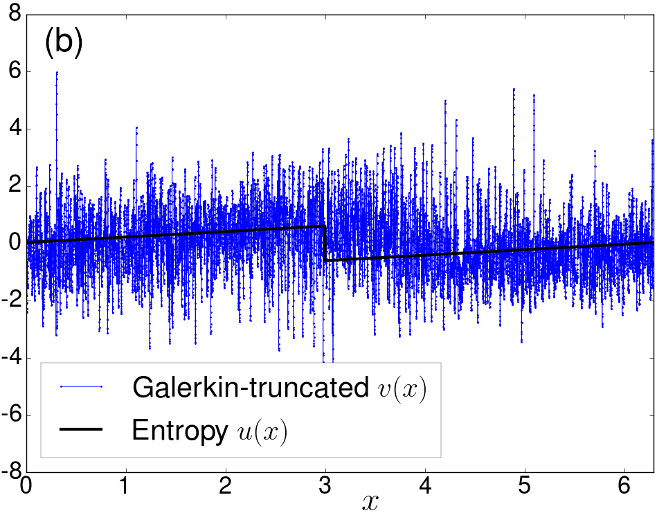
Figure 1: Representative plots, for ${K_{\scriptscriptstyle\mathrm{G}}}=1000$, of the Galerkin-truncated $v$ (blue) and entropy $u$ (black) solutions of the Burgers equation at (a) $t=0.24\gtrsim t_{*}$ and (b) $t=5.0\gg t_{*}$. For the Galerkin-truncated solution, panel (a) shows signatures of impending thermalisation through the birth of tygers while panel (b) shows the fully thermalised solutions. (We refer the reader to the youtube link https://www.youtube.com/watch?v=QiioybbVi6M for a movie of the time evolution of the Galerkin-truncated equation (and the entropy solution) with a single-mode initial condition for clarity.)

We now propose such a recipe and show how the Galerkin-truncated equation can be modified mildly to obtain solutions which do not thermalise. This allows us to obtain numerically (a) more reliable estimates of the widths of the analyticity strip and (b) weak, but dissipative, solutions (henceforth called weak-dissipative, for convenience) of inviscid equations.

The reasons which motivates this study are of course fundamentally important for the 3D Euler equations and less so for the 1D Burgers equation. However the process and mechanisms of thermalisation was best understood by resorting to the 1D Burgers equation Majda and Timofeyev (2000); Ray et al. (2011); Ray (2015); Venkataraman and Ray (2017); in the same spirit, we now outline and present results for the efficacy of the tyger purging method. At the end of this paper, we will return briefly to its applicability to the problem of the 3D Euler equation as well as contrast our approach with wavelet-based filtering techniques Pereira et al. (2013).

Thermalisation:

Let us begin with the 1D inviscid Burgers equation on a $2\pi$ periodic line

$$\frac{\partial u}{\partial t}+\frac{1}{2}\frac{\partial u^{2}}{\partial x}=0$$ (1)

augmented by the initial condition $u_{0}(x)$ which is typically a combination of trigonometric functions containing a few Fourier modes. Since we work in the space of $2\pi$ periodic solutions, we can expand the solution of Eq.(1) in a Fourier series allowing us to define the Galerkin projector $\mathrm{P}_{\!\!\!{}_{K_{\scriptscriptstyle\mathrm{G}}}}$ as a low-pass filter which sets all modes with wavenumbers $|k|>{K_{\scriptscriptstyle\mathrm{G}}}$, where ${K_{\scriptscriptstyle\mathrm{G}}}$ is a positive (large) integer, to zero via: $v(x)=\mathrm{P}_{\!\!\!{}_{K_{\scriptscriptstyle\mathrm{G}}}}u(x)=\sum_{|k|\leq{K_{\scriptscriptstyle\mathrm{G}}}}\mathrm{e}^{\mathrm{i}kx}\hat{u}_{k}$.

These definitions allow us to write the Galerkin-truncated inviscid Burgers equation

$$\frac{\partial v}{\partial t}+\mathrm{P}_{\!\!\!{}_{K_{\scriptscriptstyle\mathrm{G}}}}\frac{1}{2}\frac{\partial v^{2}}{\partial x}=0;$$ (2)

the initial conditions $v_{0}=\mathrm{P}_{\!\!\!{}_{K_{\scriptscriptstyle\mathrm{G}}}}u_{0}$ are similarly projected onto the subspace spanned by ${K_{\scriptscriptstyle\mathrm{G}}}$.

The solution of the inviscid Burgers equation (1) show one or more shocks (determined by $u_{0}(x)$), after an initial-condition dependent finite-time $t_{*}$, through which energy is dissipated for $t>t_{*}$. Theoretically, the solution to (1), for $t>t_{*}$, is obtained by adding a viscous dissipation term $\nu\frac{\partial^{2}u}{\partial x^{2}}$ with $\nu\to 0$ (the inviscid limit), which preserves the finitely many shocks of the true solution. This generalised solution, in the limit of vanishing viscosity, converges weakly to the inviscid Burgers equation and is characterised by a dissipative anomaly: energy dissipation $\epsilon$ remains finite as $\nu\to 0$.

In contrast, the Galerkin-truncated equation (2) conserves energy for all times. For initial conditions with a finite number of non-vanishing Fourier harmonic, the solution $v$ mimics rather well that of the inviscid PDE up to time $t\lesssim t_{*}$. Indeed, for $t<t_{*}$, the two solutions are essentially indistinguishable. However, when the distance of the nearest (complex) singularity of the un-truncated equation (1) is within one Galerkin wavelength ($\sim 2\pi/{K_{\scriptscriptstyle\mathrm{G}}}$) of the real domain (at time $t\approx t_{*}-{K_{\scriptscriptstyle\mathrm{G}}}^{-1/3}$), the effect of truncation becomes important.

For $t>t_{*}$, the solutions of the truncated-equation and the PDE are dramatically different: Whereas the former stays smooth, conserves energy, and start thermalising (beginning at small scales) with an (equipartition) energy spectrum $\langle|\hat{v}_{k}|^{2}\rangle\sim k^{0}$ Majda and Timofeyev (2000), the latter shows a monotonic decrease in its kinetic energy (dissipated through the shock(s)) and an associated scaling $\langle|\hat{u}_{k}|^{2}\rangle\sim k^{-2}$. (The angular brackets used in calculating the energy spectrum denotes suitable ensemble averages.) Thus thermalised solutions, inevitable in numerical solutions of the Galerkin-truncated inviscid equations, are fundamentally different from—and hence do not converge to—the un-truncated parent PDE.

We illustrate this phenomenon in Fig. 1 by showing the solutions of the Galerkin-truncated equation $v$ (in blue), with ${K_{\scriptscriptstyle\mathrm{G}}}=1000$, and the entropy solution $u$ (in black) for (a) an early time $t=0.24$ ($\gtrsim t_{*}$) and (b) at a later time $t=5.0$ ($t\gg t_{*}$); the details of such numerical simulations are given later. As discussed above, even at times very close to $t_{*}\approx 0.23$ (Fig. 1a), the two solutions show a marked difference—tygers—at points which have the same velocity as the shock (and a positive fluid velocity gradient). At even later times, (Fig. 1b) we see clear signatures of thermalisation in the truncated solution having no resemblance to the entropy solution which, as a consequence of shocks merging in time, has a saw-tooth structure with a single shock. We refer the reader to Refs. Majda and Timofeyev (2000); Ray et al. (2011); Ray (2015); Pereira et al. (2013); Venkataraman and Ray (2017); Clark Di Leoni et al. (2018) for more details and the theory of this process of thermalisation.

Tyger purging:

All of this leads us to ask if we can, without resorting to viscous dissipation, actually suppress thermalisation setting in in such truncated equations and obtain the entropy solution? The short answer is yes as we now report a novel approach—tyger purging—which, through the selective removal of a narrow, Fourier space, boundary layer near ${K_{\scriptscriptstyle\mathrm{G}}}$ (see below), at discrete time-intervals, results in the suppression of thermalisation.

The equation of motion for the purged solution $w$ is, of course, the same as that of the Galerkin-truncated equation (with the truncation wavenumber ${K_{\scriptscriptstyle\mathrm{G}}}$)

$$\frac{\partial w}{\partial t}+\mathrm{P}_{\!\!\!{}_{K_{\scriptscriptstyle\mathrm{G}}}}\frac{1}{2}\frac{\partial w^{2}}{\partial x}=0$$ (3)

augmented by an additional constraint imposed at discrete times $t_{p}=t_{*}+n\tau$ ($n$ = 0,1,2,3 …):

$$\hat{w}_{k}=0\quad\forall\quad K_{p}\leq k\leq{K_{\scriptscriptstyle\mathrm{G}}}.$$ (4)

We call this truncated equation, along with the additional purging constraint, as simply the purged equation. We note that without the additional constraint, by definition, the solution $w$ is the same as $v$ obtained from the truncated equation and hence if purging is done continuously, and not discretely, in time, we would end up solving the Galerkin-truncated equation (2) but with a truncation wavenumber $K_{p}$.

We now make the following ansätze about the inter-purging time $\tau$ and the purging wavenumber $K_{p}$:

$$\tau={K_{\scriptscriptstyle\mathrm{G}}}^{-\alpha};\quad\quad K_{p}={K_{\scriptscriptstyle\mathrm{G}}}-{K_{\scriptscriptstyle\mathrm{G}}}^{\beta};$$ (5)

with real, positive exponents $\alpha$ and $\beta$ and the immediate constraint that $\beta<1$.

Before we engage in a detailed numerical analysis, let us estimate, heuristically, optimal choices of $\alpha$ and $\beta$ keeping in mind that the purged solution $w$ must converge to the entropy solution $u$ as ${K_{\scriptscriptstyle\mathrm{G}}}\to\infty$.

For $t>t_{*}$, the entropy solution, unlike the truncated solution, is dissipative: $\varepsilon\equiv\frac{dE}{dt}<0$, where $E=\frac{1}{2}\displaystyle\sum_{k=1}^{\infty}|\hat{u}_{k}|^{2}$ is the total energy. Indeed, for times $t\sim t_{*}$, (when tygers are just born), the Galerkin-truncated Burgers equation remains conservative by the transfer—and subsequent accumulation—of kinetic energy $\propto{K_{\scriptscriptstyle\mathrm{G}}}^{-5/3}$ from the “shock” to the tygers Ray et al. (2011).

By construction, however, purging allows for a finite energy loss $\Delta E^{\rm P}\equiv\frac{1}{2}\displaystyle\sum_{k=K_{p}}^{{K_{\scriptscriptstyle\mathrm{G}}}}|\hat{w}_{k}|^{2}$ at intervals of $\tau$ resulting in a rate of loss of energy $\varepsilon^{\rm P}\equiv\frac{dE^{\rm P}}{dt}\sim\frac{\Delta E^{\rm P}}{\tau}$, where $E^{\rm P}=\frac{1}{2}\displaystyle\sum_{k=1}^{{K_{\scriptscriptstyle\mathrm{G}}}}|\hat{w}_{k}|^{2}$ is the total energy of the purged system. The choice of $\alpha$ and $\beta$ should ensure that in the limit ${K_{\scriptscriptstyle\mathrm{G}}}\to\infty$, this rate of energy loss should be ${K_{\scriptscriptstyle\mathrm{G}}}$-independent and comparable to the rate of energy loss of the entropy solution, i.e., $\varepsilon^{\rm P}=\varepsilon$.

It is hard to estimate $\Delta E^{\rm P}$ theoretically without making suitable assumptions. Since in between two purges, Eq. 3 is identical to the Galerkin-truncated equation, it is reasonable to assume that at the time of purging the solution $|\hat{w}_{k}|$ to be a combination of the one coming from the entropy solution $\hat{u}_{k}$ and a contribution from the nascent tyger. The latter, which is the deviation of the truncated from the entropy solution, was shown in Ref. Ray et al. (2011) to be confined to a narrow Fourier-space boundary layer close to and up to ${K_{\scriptscriptstyle\mathrm{G}}}$ with a form (ignoring $\mathcal{O}(1)$ constants in the prefactors as well as the argument of the exponential) $\frac{1}{{K_{\scriptscriptstyle\mathrm{G}}}}\mathrm{exp}\left[-\frac{{K_{\scriptscriptstyle\mathrm{G}}}-k}{{K_{\scriptscriptstyle\mathrm{G}}}^{1/3}}\right]$. Keeping these factors in mind, it is easy to show that $\varepsilon^{\rm P}\sim-{K_{\scriptscriptstyle\mathrm{G}}}^{\alpha+\beta-2}$. If we now demand, for convergence, that this rate be independent of ${K_{\scriptscriptstyle\mathrm{G}}}$, we obtain the constraint $\alpha+\beta=2$.

The constraint derived above is useful but it still allows considerable freedom in choosing $\alpha$ and $\beta$. However, since in between purgings the solution develops only nascent tygers, we can estimate $\beta$ independently by asking if an optimal choice of $K_{p}$ (thence, $\beta$) leads to an elimination of the boundary layer (and hence the energy content $\delta E^{\rm P}$ of the boundary layer) such that tygers are suppressed. In other words, since Galerkin-truncation leads to a transfer of energy $\sim{K_{\scriptscriptstyle\mathrm{G}}}^{-5/3}$ from the shock to the tygers resulting in an overall conservation of kinetic energy in the truncated problem, a successful purging strategy must constraint $\delta E^{\rm P}\approx{K_{\scriptscriptstyle\mathrm{G}}}^{-5/3}$ thus precisely eliminating the tygers which trigger thermalisation and hence leading to dissipative solutions. By using the functional form for the boundary layer for incipient tygers Ray et al. (2011), it is easy to show that

$$\delta E^{\rm P} \equiv \sum_{k=K_{p}}^{{K_{\scriptscriptstyle\mathrm{G}}}}|\hat{w}_{k}-\hat{u}_{k}|^{2}$$ (6)

$$\approx \sum_{k=K_{p}}^{{K_{\scriptscriptstyle\mathrm{G}}}}\frac{1}{{K_{\scriptscriptstyle\mathrm{G}}}^{2}}\mathrm{exp}\left[-\frac{{K_{\scriptscriptstyle\mathrm{G}}}-k}{{K_{\scriptscriptstyle\mathrm{G}}}^{1/3}}\right]$$

$$\sim \begin{cases}{K_{\scriptscriptstyle\mathrm{G}}}^{\beta-2}\>\>\text{for}\>\>\beta<1/3\\ {K_{\scriptscriptstyle\mathrm{G}}}^{-5/3}\>\>\text{for}\>\>\beta>1/3.\end{cases}$$

Equation (6) leads to the inevitable conclusion that the optimal choice of the purging wavenumber is one where $\beta\in[1/3,1)$ and the energy loss then is actually independent of $\beta$ and exactly the same as that which would have triggered thermalisation in the absence of purging as long as $\beta\geq 1/3$. Thus, we obtain an independent (theoretical) bound on $\beta\in[1/3,1)$ for a successful purging.

Before we turn to detailed numerical simulations to validate these ideas, we make one final remark. In numerical simulations, $\delta t$ is typically set by the resolution ${K_{\scriptscriptstyle\mathrm{G}}}$ such that $\delta t\sim\mathcal{O}({K_{\scriptscriptstyle\mathrm{G}}}^{-1})$. As we have noted before, purging if done too frequently would be akin to solving the Galerkin-truncated Burgers equation with ${K_{\scriptscriptstyle\mathrm{G}}}=K_{p}$. This implies that $\tau/\delta t\gg 1$ which, trivially, leads to $\alpha<1$. Hence, with these insights for $\alpha$ and $\beta$, we revise the constraint, estimated heuristically before, to $\alpha+\beta\lesssim 2$.

Direct Numerical Simulations:

So how effective is purging in obtaining solutions $w$ which resemble the entropy solution $u$? We answer this by resorting to extensive and detailed numerical simulation of the purged model (3) as well the Galerkin-truncated equation (2) for comparison.

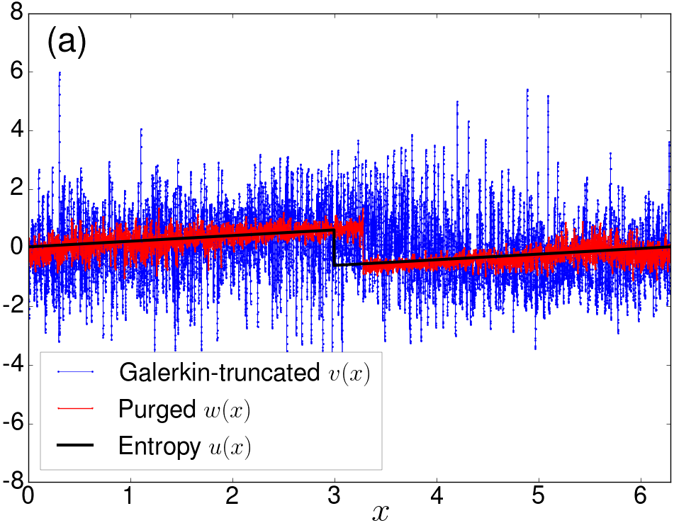
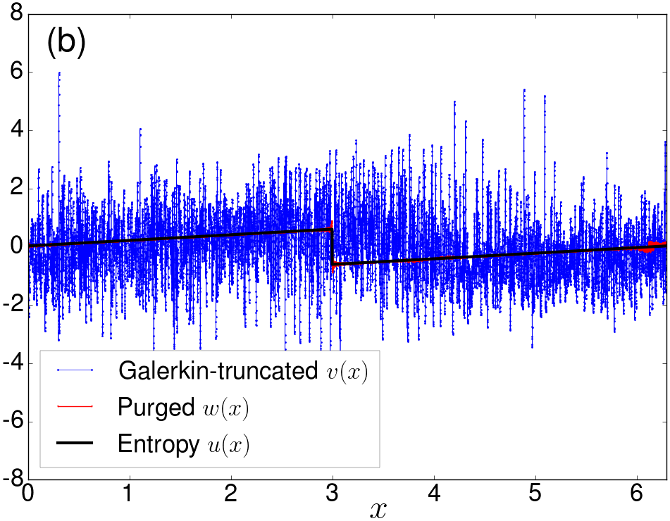
Figure 2: Representative plots, for ${K_{\scriptscriptstyle\mathrm{G}}}=1000$, of the Galerkin-truncated $v$ (blue), the entropy $u$ (black) and the purged $w$ (red) solutions of the Burgers equation at $t=5.0$ for (a) $\alpha=0.6$, $\beta=0.4$ and (b) $\alpha=\beta=0.8$. In panel (b), the purged and entropy solutions are quite close to being identical. (We refer the reader to the youtube link https://www.youtube.com/watch?v=utjyfQUuCIc for a movie of the full evolution in time of the solutions shown in panel (b).)

For the truncated and purged equations, we perform extensive direct numerical simulations, by using a standard pseudo-spectral method and a $4^{\rm th}$ order Runge-Kutta scheme for time-marching, on a $2\pi$-periodic line. We use two different sets of collocation points, namely, $N=16384$ and $N=65536$ to obtain results for ${K_{\scriptscriptstyle\mathrm{G}}}=500,1000,3000$ and 5000 (for $N=16384$) and ${K_{\scriptscriptstyle\mathrm{G}}}=8000$, and 10000 (for $N=65536$). For the purged simulations, additionally, the theoretical estimates obtained, lead us to a choice of $\beta=0.4,0.6$ and $0.8$ and for each value of $\beta$, the inter-purging time was obtained with $\alpha=0.4,0.6$, $0.8$, $0.9$, and $1.2$. (The simulations with $\alpha=0.9$ and 1.2 were performed to confirm that too frequent purgings lead to thermalised solutions once more with the effective truncation wavenumber $K_{p}$.)

The choice of time-steps in such simulations require some delicacy. For the truncated problem, since the maximum principle is violated, individual realisations of the velocity field can have excursions which are large (see Fig. 1b). Hence for the truncated simulations, as well as those where purging is ineffective in preventing thermalisation, the time-step $\delta t$ has to be kept very small. However, for the cases of successful purging (see manuscript), the maximum principle is no longer violated. Hence for these cases we are able to choose $\delta t=10^{-5}$ ($N=16384$) and $\delta t=10^{-6}$ ($N=65536$); for the analogous truncated problem (and the ones where the $\alpha$-$\beta$ combination fail to prevent thermalisation), $\delta t$ was taken to be at least two orders of magnitude smaller.

In numerical simulations, $\delta t$ is typically set by the resolution ${K_{\scriptscriptstyle\mathrm{G}}}$ such that $\delta t\sim\mathcal{O}({K_{\scriptscriptstyle\mathrm{G}}}^{-1})$. As we have noted before, purging if done too frequently would be akin to solving the Galerkin-truncated Burgers equation with ${K_{\scriptscriptstyle\mathrm{G}}}=K_{p}$. This implies that $\tau/\delta t\gg 1$ which, trivially, leads to $\alpha<1$. (We have confirmed these conjectures through several, detailed numerical simulations.)

To obtain the entropy solution $u$, we use the Fast Legendre transform as discussed in Refs. Noullez and Vergassola (1994) (see also Ref. Mitra et al. (2005)) to solve the viscous Burgers equation in the vanishing viscosity $\nu\to 0$ limit. We solve the equation on a 2$\pi$ line with periodic boundary conditions and choose $N=16384$ and $N=65536$ collocation points (for easy comparison with the truncated and purged solutions; see below). The velocity field is evolved keeping in mind that the velocity potential $\psi$ (related to the velocity field via $u=-\partial_{x}\psi$) obeys a maximum principle:

$$\psi(x,t^{\prime})={\rm max}_{y}\left[\psi(y,t)-\frac{(x-y)^{2}}{2(t^{\prime}-t)}\right].$$ (7)

Finally, we have studied the problem for several different initial conditions (all of which consist of linear combinations of trigonometric polynomials including the simplest single-mode case $\sin(x)$); we have checked that our results and conclusions are consistent for all such initial conditions. In this paper, for brevity, we present results only for the case $w_{0}=v_{0}=u_{0}=\sin(x)+\sin(2x+0.9)+\sin(3x)$.

In Fig. 2 we show representative plots, at $t=5.0$, of the Galerkin-truncated $v$ (in blue and thermalised), the entropy $u$ (in black with a prominent shock) and the purged solutions $w$ (in red) for (a) $\alpha=0.6$, $\beta=0.4$ and (b) $\alpha=0.8$, $\beta=0.8$; we set the truncation wavenumber ${K_{\scriptscriptstyle\mathrm{G}}}=1000$. We immediately see that for $\alpha=0.6$ and $\beta=0.4$ (Fig 2a), the solution $w$ approximates the entropy solution much better—in so far as picking out the ramp structure and a jump near the shock—though far from perfectly.

Remarkably, if we choose $\alpha=\beta=0.8$ (Fig 2b)—and hence much closer to satisfying the heuristic estimate $\alpha+\beta\lesssim 2$—the agreement between the purged and entropy solutions are near-perfect. Indeed the main point of departure between the two solutions seems to be close to the shock because of the ubiquitous Gibbs-type oscillations Press et al. (1992) associated with Fourier transforms of functions near discontinuities.

We have checked that for $\alpha\gtrsim 0.9$, since $\tau/\delta t\sim\mathcal{O}(1)$, the purged solutions thermalise once again as we conjectured. Hence, empirically, our extensive numerical simulations show that within the range of $\alpha$ that we study, the optimal choice is $\alpha=0.8$. Furthermore, we have confirmed that our results are largely insensitive to the choice of $\beta$ as long as its greater than 1/3.

The fact that the purged and entropy solutions seem to be in agreement, visually, suggests that the purged solution is dissipative as was anticipated, by construction, earlier. However, for this solution to actually converge to the entropy solution, the rate of dissipation should be arbitrarily close to the dissipation rate $\frac{dE}{dt}$ of the entropy solution. The most direct way to see this is to compare the total energies of the entropy $E$ and the purged $E^{\rm P}$ solutions, as a function of time, for different values of $\alpha$ and $\beta$: In Fig.  3(a) we show these results for ${K_{\scriptscriptstyle\mathrm{G}}}=1000$. We find, as was already suggested in Fig. 2, that for the optimal choice $\alpha=\beta=0.8$, the behaviour of the total energy versus time for the purged solution is identical to the one obtained from the entropy solution. The purged solutions for other $\alpha-\beta$ combinations are dissipative as well; however they dissipate energy at rates much slower than the entropy solution. Moreover, shock-mergers, as indicated by the vertical lines in the plot, and which lead to tiny kinks in the energy versus time profile, are faithfully reproduced by purged solutions for $\alpha=\beta=0.8$.

A measure of how accurately the purged solution mimics the dissipation of the entropy one, is the percentage relative error $e=\frac{E^{p}-E}{E}\times 100$ at $t=5.0$. In the inset of Fig. 3(a), we plot $e$ as a function of ${K_{\scriptscriptstyle\mathrm{G}}}$ for the most optimal purging choice ($\alpha=\beta=0.8$). Remarkably, this error $e$ decreases rapidly with ${K_{\scriptscriptstyle\mathrm{G}}}$ and for ${K_{\scriptscriptstyle\mathrm{G}}}=5000$, $e\approx 0.01\%$.

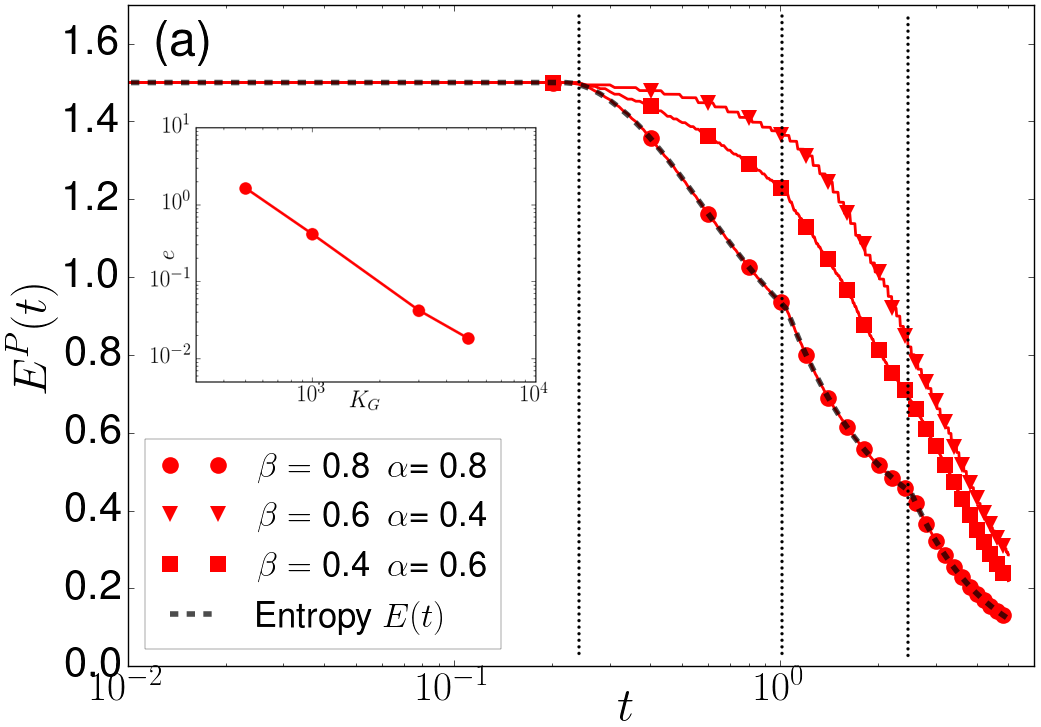
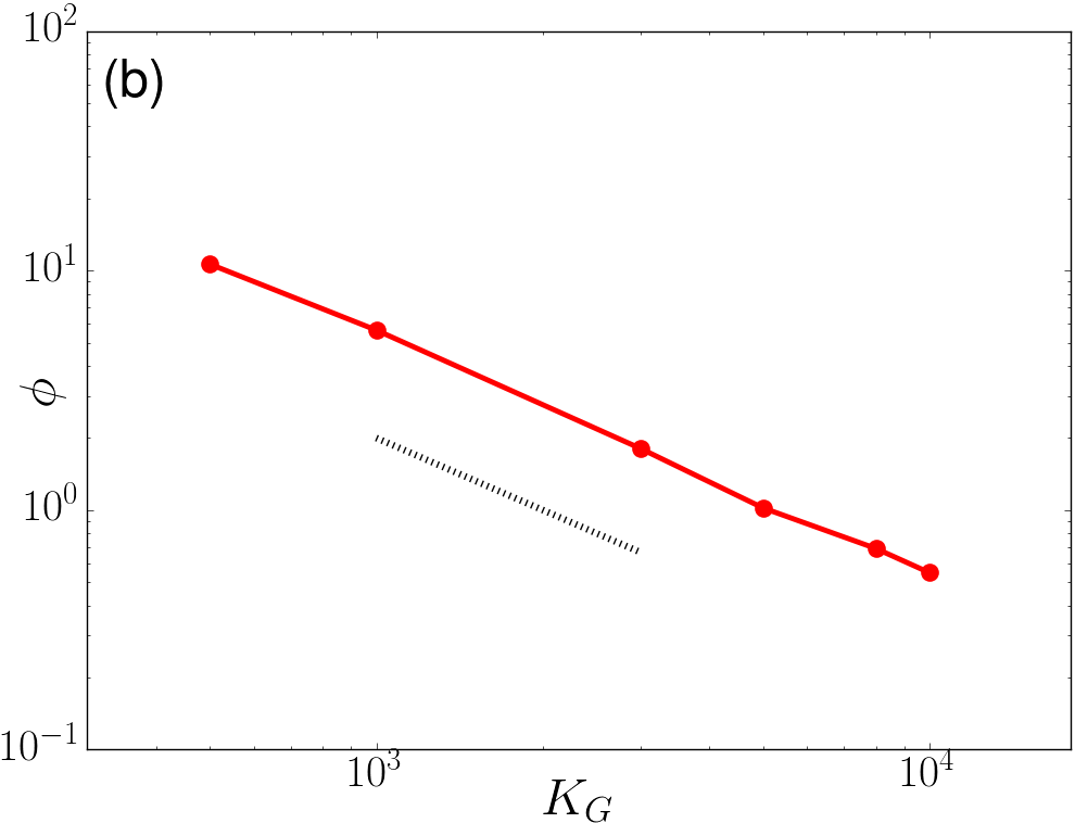
Figure 3: (a) A plot of the total energy $E^{\rm P}$ versus time, from our purged solutions  (3), for different combinations of $\alpha$ and $\beta$ and ${K_{\scriptscriptstyle\mathrm{G}}}=1000$. We also show, in black, the energy versus time plot for the entropy solution for comparison. The dashed vertical lines correspond to the times at which the shocks, three in all because of the three-mode initial conditions, form. In the inset, we plot the relative percentage error $e$ (see text) between the purged and entropy solution, for $\alpha=\beta=0.8$, at $t=5.0$, as a function of ${K_{\scriptscriptstyle\mathrm{G}}}$. (b) A plot of the $L_{2}$ norm of the percentage relative error $\phi$ (see text) for $\alpha=\beta=0.8$ as a function of ${K_{\scriptscriptstyle\mathrm{G}}}$; the dashed-line shows a power-law ${K_{\scriptscriptstyle\mathrm{G}}}^{-1}$ scaling consistent with the measured error.

All of this leads us inevitably to the important question: For $\alpha=\beta=0.8$, does the purged solution indeed converge to the entropy one as ${K_{\scriptscriptstyle\mathrm{G}}}\to\infty$? A precise way to answer this is to measure the percentage relative error (or the $L_{2}$ norm) $\phi=\sqrt{\frac{\displaystyle\sum_{i=1}^{i=N}\left[u(x_{i})-w(x_{i})\right]^{2}}{\displaystyle\sum_{i=1}^{i=N}\left[u(x_{i})\right]^{2}}}\times 100$ of the discrepancies between the solutions $u$ and $w$. Given that this is a point-wise measure, unlike the global energy measurements shown in Fig. 3(a), a sharp decrease in $\phi$ with ${K_{\scriptscriptstyle\mathrm{G}}}$ should be clinching evidence of the efficacy of our scheme. In Fig. 3(b), we show a log-log plot of $\phi$ as a function of ${K_{\scriptscriptstyle\mathrm{G}}}$ and find a steep decrease ($\phi\sim{K_{\scriptscriptstyle\mathrm{G}}}^{-1}$ indicated by the dashed line) in the relative error as a function of ${K_{\scriptscriptstyle\mathrm{G}}}$. For the large values of ${K_{\scriptscriptstyle\mathrm{G}}}$, the relative error $\phi<1\%$, reaching a value of $\phi\approx 0.5\%$ for ${K_{\scriptscriptstyle\mathrm{G}}}=10000$.

These results show that purging leads to weak-dissipative solutions which converge to the entropy solution of the parent PDE as ${K_{\scriptscriptstyle\mathrm{G}}}\to\infty$. Importantly, the discrepancy between the two solutions is already minute for values of ${K_{\scriptscriptstyle\mathrm{G}}}$ which are easily accessible. From the point of view of numerical simulations, the $\beta\geq 1/3$ condition is extremely helpful because it allows us to choose values of $\beta$ small enough such that for a given ${K_{\scriptscriptstyle\mathrm{G}}}$, the loss in resolution ${K_{\scriptscriptstyle\mathrm{G}}}-K_{p}$ through purging, is insignificantly small. As an example, for ${K_{\scriptscriptstyle\mathrm{G}}}=10000$ and $\beta=0.4$, fraction of resolution lost is about 0.3%.

Summary and Outlook:

Our results, if seen in isolation for the Burgers equation, are admittedly academic. This is because for the 1D Burgers equation, we have other ways to obtain weak-dissipative solutions as well as the widths of the analyticity strip $\delta$ analytically and numerically. Also, since for the Burgers equation the effects of truncation are felt at times very close to $t_{*}$, the $\delta$ obtained for the Burgers equation with and without purging, agree equally well with the theoretical estimate up to times very close to $t_{*}$. This is pathological to the Burgers equation and it is reasonable to conjecture that purging in the 3D Euler equation will yield more dividends. Furthermore, there is no analogue of the Fast-Legendre method for the 3D Euler equations.

It is in the light of the 3D Euler equations that this approach assumes special importance. To the best of our knowledge, till date there is no algorithm which allows, numerically, to obtain weak-dissipative solutions of the 3D Euler equation. This algorithm allows us to do exactly that. Numerically, our algorithm is trivial to implement in codes which solve the 3D Galerkin-truncated Euler equation. From earlier studies we know that the onset of thermalisation in the 3D Galerkin-truncated Euler equation is formally similar to that in the Burgers equation. Hence, the approach outlined in this paper, should allow us to implement it for the 3D Euler equations and study, numerically, dissipative solutions as well as, and possibly most importantly, take advantage of the suppression of thermalisation to finally have a firm, albeit numerical, answer for the celebrated blow-up problem. While it is true that for the 3D Euler equation, we are handicapped by a much poorer understanding of what the appropriate weak-dissipative solution ought to be, there are indeed several candidates against which our purged solutions may be benchmarked against, including the existing solutions of the incompressible Navier-Stokes equation for the largest Reynolds numbers currently attainable. We hope that our work will provide a stimulus for analogous (and important) studies of the truncated Euler equation.

Given the potential usefulness of our approach to revisit the analyticity strip method to numerically investigate the question of blow-up of the Euler equation, it might be useful to comment on recent studies of this problem. In brief, although there is some evidence that the Euler equations could avoid singularities through the formation of vortex sheets Kerr (2013); Yao and Hussain (2020a, b), other results Luo and Hou (2014); Elgindi (2019); Campolina and Mailybaev (2018) suggests that this question is far from settled. Therefore, our work, although demonstrated here for the Burgers equation, could play a role in revisiting this issue from the point of view of the width of the analyticity strip. In this context, it may be worth recalling that the one of the earliest demonstrations of the analyticity strip method for the Galerkin-truncated inviscid hydrodynamics, was for the Burgers equation Sulem et al. (1983).

Before we conclude, it is important to ask if thermalisation can be suppressed by other means (without resorting to viscosity). Purging attempts in physical space—which consists in smoothening out the tygers in physical space through local averaging—does not result in any significant suppression of thermalisation and lacks easy adaptability to different initial conditions and higher dimensional equations. A second possibility is of course the use of a hyperviscous term. This however has the drawback that we would end up solving not the inviscid equation but its viscous form and for higher-orders of the hyperviscosity—which is similar in spirit to the idea of purging—the solutions thermalise Frisch et al. (2008); Banerjee and Ray (2014); Agrawal et al. (2020). Another approach is due to Pereira, et al. Pereira et al. (2013) who showed that a wavelet-based filtering technique also leads to a suppression of the resonances leading to tygers. However, such an approach has the limitation, as mentioned by the authors themselves, that the dual operations of filtering and truncation at every time step do not commute. Hence the weak dissipation introduced in this approach is somewhat uncontrolled. To this extent we feel that the prescription we present here is most suited for generating weak-dissipative solutions and, importantly, more easily adaptable to higher-dimensional systems such as the 3D Euler equations.

Note added: We recently became aware of the work by Fehn et al. on obtaining evidence for the anomalous energy dissipation in the Euler equation Fehn et al. (2020) by using a higher order discontinuous Galerkin discretization developed by the authors. These results show promise for a numerical resolution of Onsager’s conjecture by using methods different from ours.