Continuum modelling of stress diffusion interactions in an elastoplastic medium in the presence of geometric discontinuity

Abstract

Chemo-mechanical coupled systems have been a subject of interest for many decades now. Previous attempts to solve such models have mainly focused on elastic materials without taking into account the plastic deformation beyond yield, thus causing inaccuracies in failure calculations. This paper aims to study the effect of stress-diffusion interactions in an elastoplastic material using a coupled chemo-mechanical system. The induced stress is dependent on the local concentration in a one way coupled system, and vice versa in a two way coupled system. The time-dependent transient coupled system is solved using a finite element formulation in an open-source finite element solver FEniCS. This paper attempts to computationally study the interaction of deformation and diffusion and its effect on the localization of plastic strain. We investigate the role of geometric discontinuities in scenarios involving diffusing species, namely, a plate with a notch/hole/void and particle with a void/hole/core. We also study the effect of stress concentrations and plastic yielding on the diffusion-deformation. The developed code can be from https://github.com/mrupeshkumar/Elastoplastic-stress-diffusion-coupling

Keywords chemo-mechanical coupling, material discontinuity, plasticity, stress concentration, stress diffusion interactions

1 Introduction

Diffusive species migration, such as hydrogen in steel [1], lithium in Lithium-Ion batteries (LIBs) [2], chlorine in cement [3] to name a few, cause local expansion/contraction of the materials leading to the localized chemical strains in the material. If the appropriate deformation of the solid does not accommodate these localized chemical strains, stresses referred to as diffusion-induced stress (DIS) [4] are induced. In addition to this, the localized stresses act as a driving force for the species diffusion in the materials, which is commonly referred to as stress-induced diffusion (SID) [5]. Therefore, there is a strong coupling between the diffusion and mechanics of the material, i.e., diffusion of the species causes the localized stresses, and the localized stresses also influence the diffusion of the species and vice-versa. The response of the stress-diffusion interactions can be investigated in two aspects as:

• one-way coupling: where the gradient of concentration affects the deformation field, but the localized stress state does not influence the evolution of concentration,

• two-way coupling: in addition to the influence of the gradient of local hydrostatic stress on concentration and the localized concentration also influences the localized stress state.

The presence of diffusion species, either as an external gas or resulting from electrochemical reactions leads to the severe degradation in the material properties and failure of the material [6, 7, 8, 9]. Frailure due to these multi-physical phenomenon (stress-diffusion interactions [10]) shares a major portion of material failures, viz., chloride diffusion in civil structures [3, 11, 12], hydrogen diffusion in steels [1, 13, 14, 15, 16, 17, 18, 19], aluminum [20] and NiTi alloys [21, 22, 23], bacteria diffusion in biofilms [24, 25, 26], Li diffusion in LIBs [9, 8, 27, 28].

A number of frameworks for diffusion induced deformation and fracture have been proposed assuming an elastic medium [29, 30, 31, 32, 33, 34, 35, 36, 37] and taking thermal analogy to model stress-diffusion interactions [38, 39, 40]. In the design of the system where these interactions involve, the radius and the aspect ratio of the particle plays a crucial role in the concentration as well as the fracture behavior [38, 27]. Furthermore, the fully coupled stress-diffusion interactions and the higher-order terms in the chemical potential also affects the concentration and the stress profile [41]. The geometrical, as well as the material discontinuities present in the system, also play a critical role [42, 40]. However, the assumption of an elastic medium may lead to inaccuracies in failure calculations beyond the elastic regime.

Study of failure of metallic specimens containing stress concentrations such as notches and sharp cracks showed that failure happened with restriction of a plastic zone to very near the fracture surface [43, 44, 45, 46]. The hydrogen diffusion induced localized plasticity models [47, 48, 49, 50, 51, 52] were able to show increased dislocation mobility in the presence of hydrogen diffusion, causing embrittlement. In-situ studies by Sethuraman et. al., [53] have shown that the stress exceeds yield strength during large deformation of silicon electrodes due to lithium insertion accompanied by plastic deformation. The plastic deformation helps maintain good performance and capacity during cyclic operation by reducing stress buildup [54]. Sethuraman et. al., [53] experimentally found the evolution of flow stress induced by lithiation and found a strong hysteresis which showed plastic deformation of the electrode. Motivated by these observations continuum theories [55, 56, 57, 58] have shown diffusion induced stress due to elastic-plastic deformation of the electrode material.

However, the effect of the plasticity on the one way and fully coupled stress diffusion interaction in the presence of the geometric discontinuities are still unclear. In this work, we numerically investigate the role of plasticity in one-way and two-way coupled stress-diffusion interactions. The investigation is performed for the general case of the stress-diffusion interaction framework. Hence, we have performed studies on hydrogen diffusion in steel as well as lithium diffusion in graphite anode particle.

The manuscript is structured as follows: Section 2 presents governing equations for the coupled stress-diffusion interaction in an elastoplastic medium and the numerical implementation details in an open-source finite element package FEniCS. Section 3 describes the boundary value problem. Section 4 presents the results and discussions pertaining to the chosen boundary value problem. The major conclusions are discussed in the last section.

2 Numerical formulation

In the present study we make use of a continuum model to describe the coupled diffusion deformation. We make an approximation that the diffusion in the medium and the subsequent expansion/contraction is isotropic. Consider an elasto-plastic homogeneous isotropic body occupying an open domain $\beta\subset\mathbb{R}^{2}$ and bounded by a surface $\Gamma$ with unit outward normal n. Let u : $\beta\rightarrow\mathbb{R}^{2}$ be the displacement field at any point x of the body when the body is subjected to external tractions T : $\Gamma_{t}\rightarrow\mathbb{R}^{2}$ and body forces b : $\beta\rightarrow\mathbb{R}^{2}$ and $c\ :\ \beta\rightarrow\mathbb{R}^{2}$ be the concentration field at a point x when the body is subjected to external flux $J\ :\Gamma_{J}\rightarrow\mathbb{R}^{2}$. The boundary is assumed to admit the following decompositions:

• For the elastic-plastic problem: $\Gamma=\Gamma_{u}\cup\Gamma_{t}$ and $\emptyset=\Gamma_{u}\cap\Gamma_{t}$, where $\Gamma_{u}$ is the Dirichlet boundary and $\Gamma_{t}$ is the Neumann boundary and

• For the concentration problem: $\Gamma=\Gamma_{c}\cup\Gamma_{J}$ and $\emptyset=\Gamma_{u}\cap\Gamma_{t}$, where $\Gamma_{c}$ is the Dirichlet boundary and $\Gamma_{J}$ is the Neumann boundary

The chemo-mechanical problem now simplifies to two independent variables: displacements and concentration.The boundary value problem for the coupled diffusion-deformation model in the absence of body force and the source term then becomes: find $\bm{u}:\beta\subset\mathbb{R}^{d}$ and $c:\beta\subset\mathbb{R}^{d}$.

The diffusion of the species can be defined by:

$$\frac{\partial c}{\partial t}+\mathbf{\nabla\cdot J}=0,$$ (1a)

and the mechanics of the elasto-plastic domain can be defined b:

$$\nabla\cdot\mathbf{\sigma}=\mathbf{0},$$ (1b)

subject to the following boundary conditions:

$$u=\hat{u}\hskip 14.22636pt\forall x\in\Gamma_{u},$$ (1c)

$$c=\hat{c}\hskip 14.22636pt\forall x\in\Gamma_{c},$$ (1d)

$$\bm{\sigma}\cdot\mathbf{n}=\hat{t}\hskip 14.22636pt\forall x\in\Gamma_{t},$$ (1e)

$$\mathbf{J}\cdot\mathbf{n}=\hat{\rm{J}}\hskip 14.22636pt\forall x\in\Gamma_{J},$$ (1f)

where $\bm{\sigma}$ is the Cauchy stress tensor and $\mathbf{J}$ is the flux. The thermal analogy from previous studies is used to find the influence of concentration on the stress field as:

$$\bm{\sigma}=\mathbb{C}\bigg{(}\bm{\varepsilon}-[c-c_{0}]\frac{\overline{\Omega}}{3}-\bm{\varepsilon}^{p}\bigg{)},$$ (2)

and the flux $J$ is related to the concentration and stresses by:

$${\rm{J}}=-D\bigg{(}\nabla c-\frac{\overline{\Omega}}{RT}c\nabla\sigma_{h}\bigg{)},$$ (3)

where $\mathbb{C}$ is the constitutive matrix for an linear isotropic material, $\bm{\varepsilon}$ is the total infinitesimal strain, $\bm{\varepsilon}^{p}$ is the plastic strain, $c_{0}$ is the initial or the reference concentration, $\overline{\Omega}$ is the partial molar volume, $D$ is the diffusion coefficient, $R$ is the universal gas constant, $T$ is the absolute temperature and $\sigma_{h}=\frac{1}{3}\sigma_{ii}$ is the hydrostatic stress.

2.1 Continuum mechanics modelling

In case of a coupled chemo-mechanical system the total strain increment $\dot{\varepsilon}$ can be decomposed additively. Following a small strain assumption proposed by Zhao et. al., [57] the decomposition of the strain increment can be written as,

$$\mathrm{d}\bm{{\varepsilon}}=\mathrm{d}\bm{{\varepsilon}}^{e}+\mathrm{d}\bm{{\varepsilon}}^{c}+\mathrm{d}\bm{{\varepsilon}}^{p}$$ (4)

where $\mathrm{d}\bm{{\varepsilon}}^{e},\mathrm{d}{\bm{\varepsilon}}^{c},\mathrm{d}{\bm{\varepsilon}}^{p}$ are the increment in elastic strain, diffusional strain and plastic strain respectively. The strain-displacement relationship gives,

$${\varepsilon}_{ij}=\frac{1}{2}(u_{i,j}+u_{j,i}).$$ (5)

In case of diffusion induced stress there is an additional strain due to concentration. In case of general isotropic continuum material this is written as a dilational strain rate,

$$\bm{\dot{\varepsilon^{c}}}=\dot{c}\ \frac{\overline{\Omega}}{3}\bm{I}$$ (6)

Since the material is elastically isotropic,

$$\dot{\bm{\sigma}}=\mathbb{C}^{e}:\dot{\bm{\varepsilon^{e}}}=\mathbb{C}^{e}:(\dot{\bm{\varepsilon}}-\dot{\bm{\varepsilon}}_{p}-\dot{\bm{\varepsilon}}_{c})$$ (7)

$$\bm{\dot{\varepsilon}}^{e}=\frac{1+\nu}{E}\dot{\bm{\sigma}}-\frac{\nu}{E}(\dot{\bm{\sigma}}_{kk})\mathbf{I}.$$ (8)

The isotropic $J_{2}$- flow rule gives the yield condition as,

$$f=\sigma_{e}-\sigma_{y}(\varepsilon^{p})=0$$ (9)

where $\sigma_{e}=\sqrt{\frac{3}{2}\mathbf{S}:\mathbf{S}}$ is the equivalent stress, and $\sigma_{y}$ is the yield stress, $\mathbf{S}$ is the deviatoric stress. The associated flow rule gives the plastic strain rate as,

$$\dot{\bm{\varepsilon}^{p}}=\dot{\lambda}\frac{\partial f}{\partial\bm{\sigma}}=\dot{\lambda}\frac{3\mathbf{S}}{2\sigma_{e}}$$ (10)

where $\dot{\lambda}$ is the loading parameter is found using the consistency condition $\dot{f}=0$.

The consistency condition is written as:

$$\dot{f}=\frac{3}{2}\frac{\mathbf{S}:\mathbf{\dot{\sigma}}}{\sigma_{e}}-(\frac{\partial\sigma_{y}}{\partial\varepsilon^{p}_{e}})\dot{\varepsilon^{p}_{e}}=0$$ (11)

$$\dot{\varepsilon^{p}_{e}}=\frac{3}{2}\frac{\mathbf{S}:\mathbf{\dot{\sigma}}}{(\frac{\partial\sigma_{y}}{\partial\varepsilon^{p}_{e}})\sigma_{e}}=\dot{\lambda}$$ (12)

From the plastic flow rule, we get

$$\bm{\dot{\varepsilon^{p}}}=\frac{9}{4}\frac{\mathbf{S}:\mathbf{\dot{\sigma}}}{(\frac{\partial\sigma_{y}}{\partial\varepsilon^{p}_{e}})\sigma_{e}^{2}}\bm{S}$$ (13)

where $\frac{\partial\sigma_{y}}{\partial\varepsilon^{p}_{e}}=H$ is the hardening constant for linear hardening. For numerical simplicity in the context of this paper we have implemented linear isotropic and kinematic hardening to study the evolution of plastic strain fields. For small range of plastic strains it is a reasonable assumption because the focus of this paper is mainly towards studying the influence of plastic strain in SID in the presence of geometric discontinuities. Appendix B contains the detailed derivation for the Kinematic hardening model used for numerical studies in this paper.

2.2 Weak form and finite element implementation

Consider $\bm{\mathscr{U}}$ and $\mathscr{C}$ are the displacement and the concentration trial spaces and $\mathscr{V}$and$\mathscr{P}$ are the displacement and the concentration test spaces:

$$\mathscr{U}:=\{\textbf{u(x)}\in[c^{o}(\Omega)]^{d}:\textbf{u}\in[\mathscr{W}(\Omega)]^{d}\subseteq[H^{1}(\Omega)]^{d}\hskip 5.69054pt\textbf{u}=\bm{\bar{u}}\hskip 5.69054pt\rm{on}\hskip 5.69054pt\Gamma_{u}\}$$

$$\mathscr{C}:=\{c(\textbf{x})\in[c^{o}(\Omega)]^{d}:c\in[\mathscr{W}(\Omega)]^{d}\subseteq[H^{1}(\Omega)]^{d}\hskip 5.69054ptc=\bar{c}\hskip 5.69054pt\rm{on}\hskip 5.69054pt\Gamma_{c}\}$$

$$\mathscr{V}:=\{\bm{v}(\textbf{x})\in[c^{o}(\Omega)]^{d}:\bm{v}\in[\mathscr{W}(\Omega)]^{d}\subseteq[H^{1}(\Omega)]^{d}\hskip 5.69054pt\bm{v}=\bm{0}\hskip 5.69054pt\rm{on}\hskip 5.69054pt\Gamma_{u}\}$$

$$\mathscr{P}:=\{p(\textbf{x})\in[c^{o}(\Omega)]^{d}:p\in[\mathscr{W}(\Omega)]^{d}\subseteq[H^{1}(\Omega)]^{d}\hskip 5.69054ptp=0\hskip 5.69054pt\rm{on}\hskip 5.69054pt\Gamma_{c}\}$$

where the space $\mathscr{W}(\Omega)$ includes linear displacement fields and concentration field. Upon applying the standard Galerkin procedure, the corresponding weak formulation of Equation (1a) and Equation (1b) is to find $\bm{u}\in\bm{\mathscr{U}}$ and $c\in\mathscr{C}$ such that $\forall\bm{v}\in\bm{\mathscr{V}}$ and $\forall p\in\mathscr{P}$:

$$a(\bm{u},\bm{v})=\ell(\bm{v}),$$ (14a)

$$b(c,p)=\ell(p),$$ (14b)

where

$$a(\bm{u},\bm{v},c)=\int_{\Omega}\bm{\sigma}(\bm{u},c):\bm{\varepsilon}(\bm{v})\hskip 2.84526pt\rm{d}\Omega,$$ (15a)

$$\ell(\bm{v})={\int_{\Gamma}}_{t}\bm{\hat{t}}\cdot\bm{v}\hskip 2.84526pt\rm{d}\Gamma,$$ (15b)

$$b(c,p,\bm{\sigma}_{h})=\int_{\Omega}\frac{\partial c}{\partial t}p\hskip 2.84526pt\rm{d}\Omega+\int_{\Omega}\left(\nabla\textit{p}\right)^{\rm{T}}\nabla c\hskip 2.84526pt\rm{d}\Omega-\int_{\Omega}\left(\nabla\textit{p}\right)^{\rm{T}}c\nabla\bm{\sigma}_{h}\hskip 2.84526pt\rm{d}\Omega,$$ (15c)

$$\ell(p)=\int_{\Gamma}\bm{J}\cdot\bm{n}\hskip 2.84526ptp\hskip 2.84526pt\rm{d}\Gamma.$$ (15d)

For the temporal discretization, we partition the time interval of interest $\tau$ into $n_{\rm{step}}$ sub-intervals and focus on typical time slab $\left[t_{i},t_{i+1}\right]$. To approximate the time derivative of concentration $c$, we apply a first order finite difference scheme as,

$$\frac{\partial c}{\partial t}=\frac{c_{i+1}-c_{i}}{\Delta t}$$ (16)

, where $\Delta t=t_{i+1}-t_{i}>0$ is the current time increment. We employed the backward Euler time integration scheme and evaluate the discrete set of governing equations at current time step $t_{i+1}$.

FEniCS [59] is a very powerful finite element package which translates the weak form of the coupled differential equations into the corresponding finite element solution. The total residual from $F$ used in the FEniCS is given as,

$$F=a(\bm{u},\bm{v})-\ell(\bm{v})+b(c,p)-\ell(p).$$ (17)

The Newton raphson scheme in the FEniCS can be called as, solve(F==0, w, bcs), where w is the solution space and bcs are the boundary conditions. Algorithm 1, shows the solution procedure followed in the numerical analysis.

initialize displacement, concentration fields at time $t_{i}$- $\bm{u}_{i}$, $c_{i}$

while $t_{i+1}<t_{end}$ do

       Converged displacement, concentration fields, at time $t_{i}$ - $\bm{\mathrm{u}}_{i}$, $\bm{\mathrm{c}}_{i}$

       Update strain rates $\bm{\mathrm{\dot{\varepsilon}}}_{i}$, $\bm{\mathrm{\dot{\varepsilon^{c}}}}_{i}$ using backward Euler scheme

       if  Yield condition satisfied, $f\geq 0$ then

            Update plastic strain rate $\bm{\mathrm{\dot{\varepsilon^{p}}}}_{i}$

       end if

      Update corresponding stress rate, $\bm{\mathrm{\dot{\sigma}}}_{i}$ and stress field, $\bm{\mathrm{\sigma}}_{i}$ using backward Euler scheme.

       Solve for $F=0$ using Newton raphson scheme for displacement and concentration fields, at time $t_{i+1}$ - $\bm{\mathrm{u}}_{i+1}$, $\bm{\mathrm{c}}_{i+1}$

       Update solution for $t_{i}$ to solution at $t_{i+1}$

end while

Algorithm 1 Solution algorithm

3 Problem definition

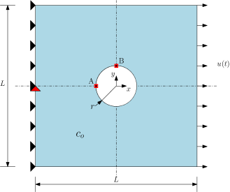
(a)

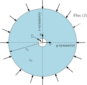
(b)

Figure 1: (a) Schematic representation of a rectangular domain with a central hole of radius $r$ subjected to uniaxial displacement $u(t)$ at the right edge and fixed at the left edge. The points A, and B are the points of interest for the study. (b) A circular domain of radius $r_{o}$ with a central void of radius $r_{i}$ subjected to a radial flux $J$. Both the domains have an initial concentration $C_{0}$.

We analyse two boundary value problems in this study:

• a plane strain domain with a circular hole of radius $r$ as shown in Figure 1a. The effects of plasticity and singularity on stress-diffusion interactions is investigated. The radius of the hole $r$ has been varied in order to vary the singularity level on the boundary of the hole. The initial or the reference concentration, $c_{0}$ is assumed to be zero. The initial and the boundary conditions for the system are $\forall\ t>0$,

  $$u_{x}(-L/2,y,t)=0,\hskip 14.22636ptu_{y}(-L/2,0,t)=0,\hskip 14.22636ptu_{x}(L/2,y,t)=\bar{u}(t),\hskip 14.22636ptc(-L/2,y,t)=1.$$

• a plane strain cylindrical domain of outer radius $r_{o}$ and inner radius $r_{i}$, see Figure 1b. The initial concentration $c_{o}$ is assumed to be zero and outer boundary is subjected to constant Flux $J$.

Table 1: Material parameters for Li in graphite system [60]

Property	Value
Young’s modulus $(\rm{E})$	$19.25\rm{GPa}$
Poisson’s ratio $(\nu)$	$0.3$
Diffusivity $(\rm{D})$	$3.9\times 10^{-14}\rm{m^{2}/s}$
Temperature $(\rm{T})$	$300\rm{K}$
Partial molar volume $(\Omega)$	$4.17\times 10^{-6}\rm{m^{3}/mol}$

The material parameters used for both the boundary value problem is tabulated in the Table 1, which corresponds to the Li in the graphite system [60].

4 Results and Discussions

In this section, the results pertaining to the interactions between stress and concentration will be presented. We analyse problems with increasing complexities. first, we start with (Section 4.1) the analysis of the two-dimensional diffusion in pure elastic medium and validation with the analytical solution. Then we validate the current implementation (one-way coupled elasto-plastic simulation) with the commercial available finite element package Abaqus [61] and analyzed the effect of two-way coupling. The effect of plastic yielding on the stress-diffusion interaction will be discussed in the Section 4.2. The effect of one-way and two-way for the particle model with and without the plasticity for applied flux is investigated in the Section 4.3.

4.1 Implementation validation with the analytical model and the effect of plasticity

The implemented model is validated with the analytical solution available for the pure diffusion. The analytical solution for a circular hole of radius $a$ in an infinite body under plane deformation and tensile forces $p$, the hydrostatic stresses in polar coordinates $(r,\beta)$ are given by [51]:

$$\sigma_{h}=\dfrac{(1+\nu)p}{3}\bigg{(}\dfrac{2R^{2}}{r^{2}}cos2\beta-1\bigg{)},$$ (18)

and the concentration is given by:

$$C(r,\beta)=C_{0}e^{\left(\ -k\frac{2(1+\nu)R_{0}^{2}p}{3r^{2}}cos2\beta+C_{0}Q\right)}e^{\left[-LambertW\left(C_{0}e^{\left(-k\frac{2(1+\nu)R_{0}^{2}p}{3r^{2}}cos2\beta+C_{0}.Q\right)}\right)\right]}$$ (19)

where $k=\frac{V_{H}}{RT},Q=\frac{2\alpha_{c}V_{H}E}{9(1-\nu)RT}$, $LambertW(x)$ is the Lambert function.

4.1.1 Diffusion in the pure elastic medium

In order to validate the FEniCS implemented model, a rectangular domain with a circular hole with aspect ratio (L/r) = 10 & 20, where L is the length of the domain and $r$ is the radius of the hole, is considered. The initial and the boundary conditions for the system are $\forall\ t>0$,

$$\sigma_{x}(-L/2,y,t)=-p,\hskip 14.22636pt\sigma_{x}(L/2,y,t)=p,\hskip 14.22636ptc(x,y,t=0)=C_{0}\text{ (outside the hole)},$$

where $p$ is the uni-axial tensile load of 100 MPa magnitude. The boundary of the domain is assumed insulated such that species can not leave the system. The effect of plasticity is neglected and material is assumed to be perfectly elastic for comparison. The material properties of the specimen is tabulated in the Table 2.

Table 2: Properties of the steel specimen used for analytical and numerical comparison[51]

Property	Value
Young’s modulus $(\rm{E})$	$210\rm{GPa}$
Poisson’s ratio $(\nu)$	$0.3$
Diffusivity $(\rm{D})$	$1.27\times 10^{-8}\rm{m^{2}/s}$
Temperature $(\rm{T})$	$300\rm{K}$
Partial molar volume $(\Omega)$	$1.96\times 10^{-6}\rm{m^{3}/mol}$

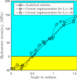
(a)

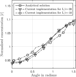
(b)

Figure 2: Plate with circular hole: (a) hydrostatic stress, $\sigma_{h}$ and (b) normalized concentration as a function of angle about the center, $\pi=3.14$

Figure 2 compares the numerical solution for the concentration and the hydrostatic stress with the analytical model as a function of angle about the center. The implemented FEniCS numerical results shows the decent match with the analytical solution as the aspect ratio of the problem domain increases. The state of stress changes from compressive to tensile as the angle increases as shown in Figure 2a. The maximum hydrostatic stress is at $\beta=\pi/2$ whereas the minimum hydrostatic stress is at $\beta=0$. The distribution of the concentration species follows the distribution of the hydrostatic stress. The tensile sites are capable of holding more diffusion species than the compressive sites and hence the concentration at the tensile sites is more, which is evident from the Figure 2b.

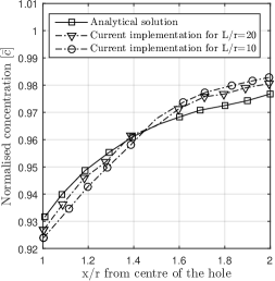
(a)

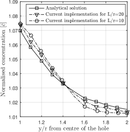
(b)

Figure 3: Plate with a circular hole: normalized concentration along the line (a) $\beta=0$ and (b) $\beta=\pi/2$

Now, Figure 3 compares the concentration of species along the line at $\beta=0$ and $\beta=\pi/2$. The concentration level shows a decent match with the analytical model for both along the line at $\beta=0$ and $\beta=\pi/2$. Moreover, The concentration increases as the distance from the compressed region increases as shown in Figure 3a and decreases as the distance from the tensile region increases as shown in Figure 3b. Hence singularity level at the localized sites plays a critical role on the concentration build up.

4.1.2 Effect of plastic yielding on the concentration

We assume a plane strain plate with an elastoplastic medium is subjected to the same boundary conditions as presented in the Section 4.1.1. Figure 4 shows the hydrostatic stress and the concentration around the hole. The plastic yielding reduces the magnitude of the hydrostatic stress at the compressive as well as the tensile states as shown in Figure 4a.

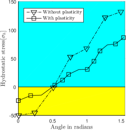
(a)

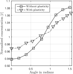
(b)

Figure 4: Plate with circular hole: (a) hydrostatic stress, $\sigma_{h}$ and (b) normalized concentration as a function of angle about the center, $\pi=3.14$

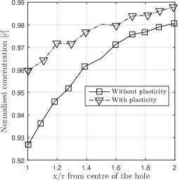
(a)

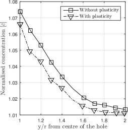
(b)

Figure 5: Plate with a circular hole: normalized concentration along the line (a) $\beta=0$ and (b) $\beta=\pi/2$

The distribution of the concentration species follows the distribution of the hydrostatic stress which has less magnitude than the pure elastic medium at the tensile as well as the compressive sites. The reduced magnitude of tensile stress pulls lesser concentration of diffusing species from the surroundings and the reduced magnitude of compressive stress pushes through lesser concentration species to the surrounding and hence species concentration at the tensile sites is less and more in the compressive sites in elasto-plastic medium than purely elastic medium as shown in Figure 4b. Figure 5 shows the distribution of the concentration along line $\beta=0$ and $\beta=\pi/2$ with and without plasticity effect. The concentration level increases as the distance from the singular region increases for elastic as well as elasto-plastic medium for the line $\beta=0$. The line $\beta=0$ is in compressive zone and hence the concentration level is more for the elasto-plastic medium than pure elastic medium as shown in Figure 5a. The concentration level along $\beta=\pi/2$ decreases for both elastic as well as elastoplastic medium as the distance from the singular region increases but the magnitude of the concentration level is less for the elastoplastic medium as region $\beta=\pi/2$ is in tensile state of stress as shown Figure 5b.

The introduction of the diffusing species in or out of the media affects the magnitude and evolution of the plastic yielding at tensile and compressive region respectively. Figure 6 shows the equivalent plastic strain at normalized time 0.7 along $\beta=0,\pi/4$ and $\pi/2$. The line along $\beta=0$ starts with the compressive zone which implies a reduction of concentration of diffusive species which reduces the stress concentration and hence shows lesser plastic yielding. The line along $\beta=0$ starts with the compressive zone which implies a accumulation of concentration of diffusive species which increases the tensile stress and hence shows higher plastic yielding. Away from the singularity the effect of plastic yielding decreases with distance.

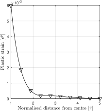
(a)

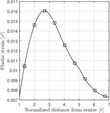
(b)

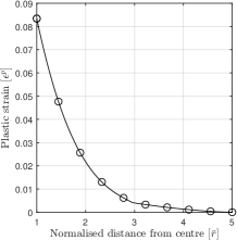
(c)

Figure 6: Plate with a circular hole: Plastic strain along the line (a) $\beta=0$, (b) $\beta=\pi/4$ and (c) $\beta=\pi/2$

4.2 Analysis of boundary value problem a, see Figure 1a

Before analyzing the problem in detail, we have verified our FEniCS implementation with Abaqus. In Abaqus, we have used coupled-thermal analysis which is one-way coupled analysis in our context. The analysis is performed for the elastoplastic material. Figure 7 shows the concentration at points A and B with respect to the normalized time for one-way coupled problem. The point A is nearer than the point B from the left boundary and hence the concentration is higher at point A at any point of time. However, both points reaches steady state concentration level at the end of the simulation which is consistent with the work of Natarajan et. al.,[42]. This is due to the fact that the effect of stresses in not considered in one-way coupling. Our implementation results shows excellent agreement with the Abaqus results, see Figure 7. Figure 8 also compares the hydrostatic stress evolution at points A and B with respect to the normalized time. The implemented model is able to capture tensile to compressive state at point A and compressive to tensile state at point B which is also evident from the Abaqus results.

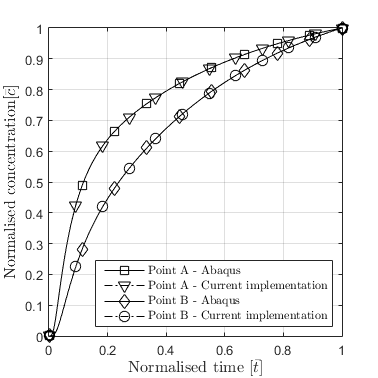
(a)

Figure 7: Plate with a hole: normalized concentration with respect to normalized time at points A and B for one-way coupled system

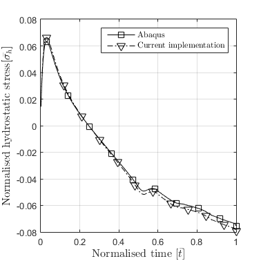
(a)

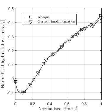
(b)

Figure 8: Plate with a hole: evolution of normalized hydrostatic stress, $\sigma_{h}$ with respect to the normalized time at point (a) A (b) B for for one-way coupled system.

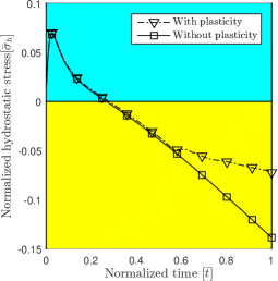
(a)

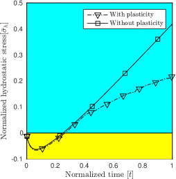
(b)

Figure 9: Two way coupling - Normalized hydrostatic stress, $\bar{\sigma_{h}}$ as a function of normalized time at point (a)A (b) B for with and without plasticity.

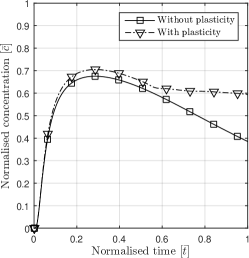
(a)

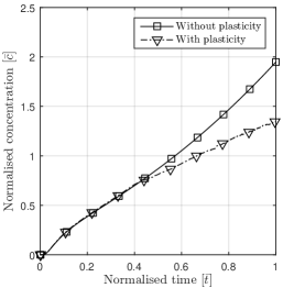
(b)

Figure 10: Two way coupling- Normalized concentration vs Normalized time at point (a) A (b) B for a plate with a hole with and without plasticity

In order to illustrate the effect of plasticity on the stress-diffusion interactions, we compare the results of pure elastic and elastoplastic material and two-way coupled model. Figure 9 shows the hydrostatic stress evolution at different points as a function of normalized time for pure elastic as well as elastoplastic material. The state of stress at a point A is initially tensile but changes to compressive due to continuous pulling and concentration evolution in the domain. Moreover, the state of stress changes from compressive to tensile at point B. The plastic yielding significantly reduces the stress level in the tensile site (point B) and makes it less compressive in the compressive site (point A). The level of concentration in the domain depends on the gradient of concentration as well as the localized state of stress. Tensile sites are capable to hold more concentration whereas compressed sites tries to push the concentration to near by sites. Figure 10a shows the concentration evolution at the point A. Initially the state of stress at this point is tensile and gradient of concentration is also present, the concentration of species increases with respect to time. But as the state of stress changes from tensile to compressive (at normalized time 0.3 please refer Figure 9a), the point A is no longer able to take/hold the concentration of the species and hence magnitude of concentration of the species starts decreasing. However in an elastoplastic medium the compressive stress is reduced due to plastic yielding which reflects on the higher concentration compared to pure-elastic medium. In contrast at point B, the level of concentration increases monotonically as shown in Figure 10b. The initial increase in the concentration level is due to the gradient of the concentration and later gradient of hydrostatic term predominates which is responsible for the increase of concentration level. Once again, however we notice that the tensile stress reduction due to plastic yielding reduces concentration of the diffusing species at point B in an elastoplastic medium. Hence it can be concluded that the plastic yielding in the system plays a critical role in determining the steady state behaviour.

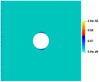
(a)

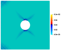
(b)

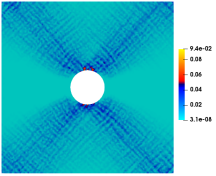
(c)

Figure 11: One-way coupling - Plastic strain contours at normalized time (a) 0.30 (b) 0.4 (c) 0.7

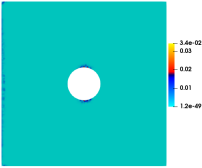
(a)

(b)

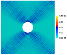
(c)

Figure 12: Two-way coupling - Plastic strain contours at normalized time (a) 0.35 (b) 0.4 (c) 0.7

Figures 11 and 12 shows the plastic strain evolution for one-way and two-way coupled system at different normalized time. In the two-way coupled system, there is a local stress relaxation (analogous to expansion due to temperature rise [42]) and therefore, it leads to a lower stress concentration around the singularity. The equivalent plastic strain due to tension around the hole is lesser in case of two-way coupled system than the one-way coupled system, see Figures 11 and 12. This provides evidence of the reduced tensile stress concentration and the concentration of the species due to the relaxation effect in case of two-way coupled system.

one-way coupled system                 two-way coupled system

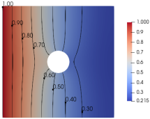
(a)

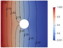
(b)

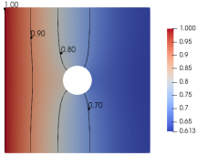
(c)

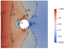
(d)

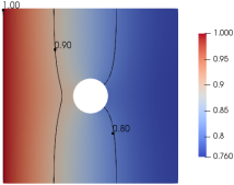
(e)

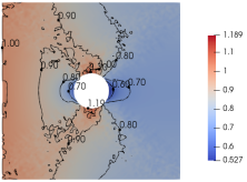
(f)

Figure 13: Plate with hole: concentration contour at normalized time (a) 0.3 (b) 0.4 and 0.7 for one-way and two-way coupled system.

Figure 13 compares the concentration contour of one-way and two-way coupled system at different normalized time. The asymmetry of the concentration in the case of one-way coupling is only due to the hole present in the system, see Figures 13a,13c and 13e. Whereas the asymmetry of the concentration is due to both hole and the stresses, see Figures 13b, 13d and 13f. In the case of Two-way coupling, the location of the concentration build up is not the same as compared to the one way coupling. Although the point A is nearer to the point B from the left edge, the concentration build up is more at the point B. This observation is opposite to our earlier observation in one-way coupling. The main reason behind the different build up profile is due to stress induced diffusion effect in the case of two-way coupling. Hence in studying the stress diffusion interactions consideration of the effect of stresses on the singularities is mandatory. The effect is more dominant if the high stress gradient present in the domain as in case of stress singularities due to discontinuities.

4.3 Analysis of boundary value problem b, see Figure 1b

In the recent times, hollow nano-anode structures have attracted attention because of their extra space to accommodate the volume expansion/contraction due to charge and discharge and hence increases the cyclic performance. We attempt to understand the influence a void in a particle on the chemo-mechanical behaviour for elasto-plastic material.

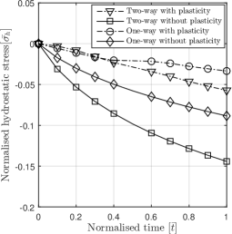
(a)

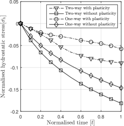
(b)

Figure 14: Hydrostatic stress at outer radius (a) without void (b) with void

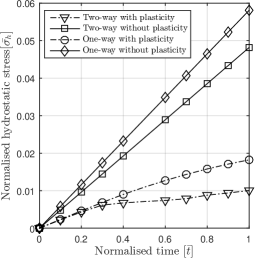
(a)

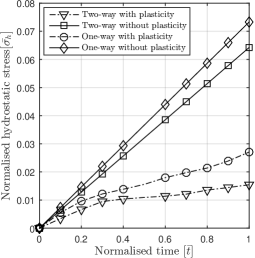
(b)

Figure 15: Hydrostatic stress at inner radius (a) without void (b) with void

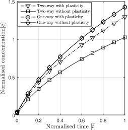
(a)

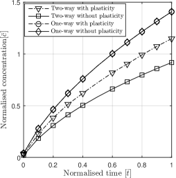
(b)

Figure 16: Concentration at outer radius (a) without void (b) with void

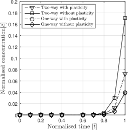
(a)

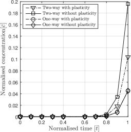
(b)

Figure 17: Concentration at inner radius (a) without void (b) with void

Due to the incoming flux (charging operation) on the boundary, the outer surface of the particle undergoes compression and the inner surface of the particle undergo tension, see Figures 14 and 15. From our earlier observation these stresses consequently affects the diffusion process for the two-way coupled system. At the outer radius(compressive region) the two-way coupled system shows lesser concentration of diffusive species as compared to the one-way coupled system whereas at the inner radius (tensile region) the two-way coupled system shows higher concentration as compared to the one-way coupled system, as shown in Figures 16 and 17.

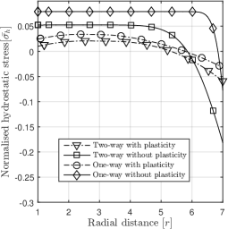
(a)

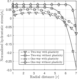
(b)

Figure 18: Hydrostatic stress along radius (a) without void (b) with void

The stress in elastoplastic medium is lowered than in pure elastic medium due to plastic yielding. The plastic yielding lowers the tensile stress at the inner radius (tensile region) and hence causes an outflux leading to a decrease in concentration compared to pure elastic media, see Figure 17. The inverse effect occurs at the outer radius (compressive region), where a reduction in compressive stress due to plastic yielding causes an influx of diffusing species leading to an increase in concentration, see Figure 16.

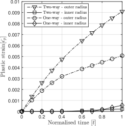
(a)

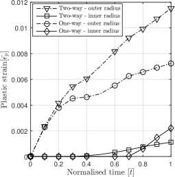
(b)

Figure 19: Plastic strain at outer and inner radius (a) without void (b) with void

When comparing the concentration in one-way coupled model with and without plasticity as shown in Figures 16 and 17, we see negligible difference because the stress field does not influence the diffusion process in that case. We also note that the compressive stress (at the outer radius) in case of two-way coupled system is more than the one-way coupled system and the tensile stress (at the inner radius) is less in case of two-way coupled system is more than the one-way coupled system, as shown in Figures 14 and 15. This is due to the stress-relaxation effect caused by flux of diffusing species out of the compressive region and into the tensile region respectively as discussed in the previous section. The plastic yielding reduces the overall singularity in stress due to compression and tension in both one-way and two-way coupled systems. However due to the stress-relaxation effect in two-way coupled system we see (in figure 19) higher plastic yielding at the outer radius and lower plastic yielding at the inner radius for two-way coupled system when compared to one-way coupled system. From the concentration contour plots as shown in Figures 20, 21 22, 23, concentration is lesser at the outer radius and more at the inner radius in case of the two-way coupled system when compared to one-way system which further illustrates the stress-relaxation effect in two-way system. Along with this, Figure 18 gives us a qualitative understanding about the effect of induced stress on diffusion. We observe that due to a high gradient in concentration at the outer radius, the hydrostatic stress and its gradient is also high. As we move closer to the centre the concentration gradient reduces, leading to a smaller/no gradient in the hydrostatic stress. This is similar to effect observed by Swaminathan et. al., [60].

In order to illustrate the influence of discontinuities, we introduce a void in the particle model. We observe that introduction of the void in the coupled diffusion-deformation process increases the compressive stress at the outer radius (see, Figure 14) and the tensile stress at the inner radius, see Figure 15. This consequently reflects on the plastic yielding and affects the diffusion process and vice versa, see Figure 19. At the outer radius (compressive region) the two-way coupled system shows a reduction in the concentration due to an increase in compressive stress (see, Figure 16). At the inner radius (tensile region) the two-way coupled system shows an increase in concentration due to an increase in compressive stress (see, Figure 17). The effect of discontinuity on the concentration is negligible in one-way coupled model as expected because the stress does not influence the diffusion process. The concentration contour plots (see, Figures 20, 21 22, 23) further provide evidence to illustrate this effect.

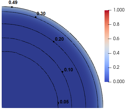
(a)

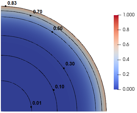
(b)

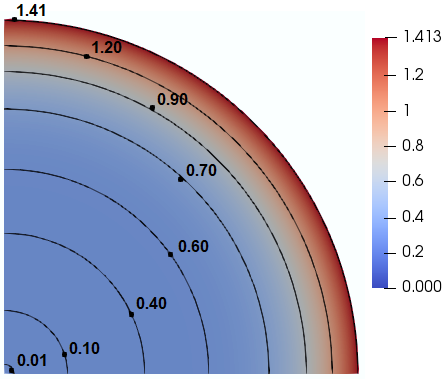
(c)

Figure 20: One way coupling - Concentration contours at normalized time (a) 0.2s (b) 0.5s (c) 1s

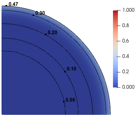
(a)

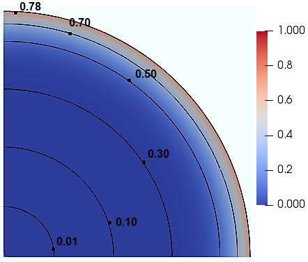
(b)

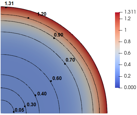
(c)

Figure 21: Two way coupling - Concentration contours at normalized time (a) 0.2s (b) 0.5s (c) 1s

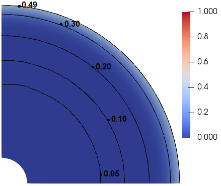
(a)

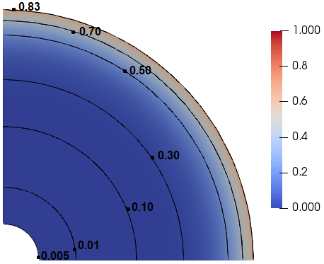
(b)

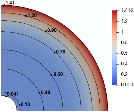
(c)

Figure 22: One way coupling - Concentration contours at normalized time (a) 0.2s (b) 0.5s (c) 1s

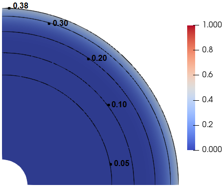
(a)

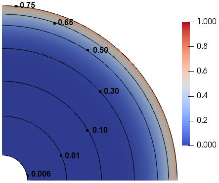
(b)

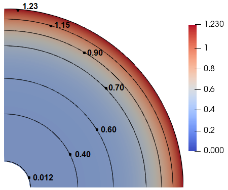
(c)

Figure 23: Two way coupling - Concentration contours at normalized time (a) 0.2s (b) 0.5s (c) 1s

5 Concluding remarks

In this paper, the effect of stress diffusion interactions in an elasto-plastic material with/without discontinuity using a coupled chemo-mechanics system has been investigated. Moreover, the effect of the fully coupled system over the one-way coupled system is studied systematically for the general framework of the species diffusion in the solid (hydrogen diffusion in steel as well as Li ion diffusion the LIBs). The concentration buildup in the one-way coupled system only depends on the distance from the source where as in two-way coupling the concentration build up depends not only on the distance but the local state of the stress. Study reveals also that the state of stress in the domain is the determining factor in studying the chemo-mechanics system and may change the concentration buildup point (depends on tensile and compressive site). The plastic yielding at the tensile sites reduces the local diffusion species and same affects in reverse for the compressive sites. Moreover, the discontinuities in the domain severely affects the stress-diffusion interactions.

Appendix A: non-dimensionalization of equations

Consider the balance of diffusion species Eqn. (1a),

$$\frac{\partial c}{\partial t}-D\nabla_{x}c+\frac{D\Omega}{\rm{RT}}c\nabla_{x}\bm{\sigma}_{h}=0.$$ (20)

The Equation (20) is non-dimensionalized by assuming a new set of dimensionless variables for space ($L^{*}$), time ($t^{*}$), concentration ($c^{*}$) and the hydrostatic stress ($\bm{\sigma}_{h}^{*}$) :

$$\hat{x}=\frac{x}{L^{*}},\,\hat{t}=\frac{t}{t^{*}},\,\hat{c}=\frac{c}{c^{*}},\,\hat{\bm{\sigma}}_{h}=\frac{\bm{\sigma}_{h}}{\bm{\sigma}^{*}_{h}}.$$ (21)

Now, using the chain rule and substituting new variables in terms of ($\cdot^{*}$) in Eqn. (20) one can get,

$$\frac{c^{*}}{t^{*}}\frac{\partial\hat{c}}{\partial\hat{t}}-\frac{c^{*}}{{L^{*}}^{2}}\nabla_{\hat{x}}c+\frac{c^{*}}{{L^{*}}^{2}}\frac{D\Omega}{\rm{RT}}c^{*}\hat{c}\nabla_{x}\bm{\sigma}_{h}=0.$$ (22)

Now multiply $t^{*}$ in Eqn. (22),

$$c^{*}\frac{\partial\hat{c}}{\partial\hat{t}}-\frac{c^{*}t^{*}}{{L^{*}}^{2}}\nabla_{\hat{x}}c+\frac{c^{*}t^{*}}{{L^{*}}^{2}}\frac{D\Omega}{\rm{RT}}c^{*}\hat{c}\nabla_{x}\hat{\bm{\sigma}_{h}}=0.$$ (23)

On assuming, $c^{*}=1$, $\frac{Dt^{*}}{{L^{*}}^{2}}=1$, $\dfrac{\Omega\bm{\sigma}_{h}}{RT}=1$ and upon back substitution in Eqn. (21) we get $\hat{t}=t\frac{l^{2}}{D}$, $\hat{c}=\frac{c}{c_{\rm{max}}}$, $\hat{\bm{\sigma}}_{h}=\bm{\sigma}_{h}\dfrac{\rm{RT}}{\Omega}$.
Hence, non-dimensionalized equation is given as,

$$\dfrac{\partial\hat{c}}{\partial\hat{t}}-\nabla_{\hat{x}}\hat{c}+\hat{c}\nabla_{\hat{x}}\hat{\bm{\sigma}}_{h}=0.$$ (24)

Appendix B: incremental equations for numerical scheme

In this appendix we see the numerical procedure for coupled deformation-diffusion using a Kinematic hardening model. Kinematic hardening model uses a back stress, $\beta_{ij}$ , which results in a dependence on loading in the hardening model.

The yield condition in case of Kinematic hardening can rewritten as:

$$f=\frac{1}{2}(\bm{S}_{ij}-\bm{\beta}_{ij})(\bm{S}_{ij}-\bm{\beta}_{ij})-\frac{1}{3}\sigma_{y}^{2}$$ (25)

where $\bm{S}_{ij}=\bm{\sigma}_{ij}-\frac{1}{3}\sigma_{kk}\bm{\delta}_{ij}$ is the deviatoric stress. We aim at modelling the back stress, $\beta_{ij}$. We use a linear hardening model governed by:

$$\bm{\dot{\beta_{ij}}}=h\dot{\bm{\varepsilon^{p}}}_{ij}$$ (26)

where h is the hardening constant. Using the associated flow rule,

$$\bm{\dot{\beta_{ij}}}=h\dot{\lambda}(\bm{\sigma}_{ij}-\bm{\beta}_{ij})$$ (27)

Making use of the consistency condition,

$$\dot{f}=0=\frac{\partial f}{\partial\bm{\sigma}_{ij}}\dot{\bm{\sigma}_{ij}}+\frac{\partial f}{\partial\bm{\beta}_{ij}}\dot{\bm{\beta}_{ij}}=(\bm{S}_{ij}-\bm{\beta}_{ij})\dot{\bm{S}_{i}j}-(\bm{S}_{ij}-\bm{\beta}_{ij})\dot{\bm{\beta}_{ij}}$$ (28)

$$(\bm{S}_{ij}-\bm{\beta}_{ij})\dot{\bm{S}_{i}j}=(\bm{S}_{ij}-\bm{\beta}_{ij})\dot{\bm{\beta}_{ij}}$$ (29)

$$(\bm{S}_{ij}-\bm{\beta}_{ij})\dot{\bm{S}_{ij}}=h\dot{\lambda}(\bm{S}_{ij}-\bm{\beta}_{ij})(\bm{\sigma}_{ij}-\bm{\beta}_{ij})$$ (30)

$$\dot{\lambda}=\frac{(\bm{S}_{ij}-\bm{\beta}_{ij})\dot{\bm{S}_{ij}}}{h(\bm{S}_{ij}-\bm{\beta}_{ij})(\bm{\sigma}_{ij}-\bm{\beta}_{ij})}=\frac{(\bm{S}_{ij}-\bm{\beta}_{ij})\dot{\bm{S}_{ij}}}{\frac{2h}{3}\sigma_{y}^{2}}$$ (31)

In order to eliminate the rate of stress, we use again Hooke’s law,

$$\dot{\lambda}=\frac{(\bm{S}_{ij}-\bm{\beta}_{ij})\mathbb{C}_{ijkl}(\dot{\bm{\varepsilon}_{kl}}-\dot{\bm{\varepsilon^{p}}_{kl}}-\dot{\bm{\varepsilon^{c}}_{kl}})}{\frac{2h}{3}\sigma_{y}^{2}};\;\;\;\;\dot{\bm{\varepsilon^{p}}_{ij}}=\dot{\lambda}(\bm{S}_{ij}-\bm{\beta_{ij}});\;\;\;\;\dot{\bm{\beta}_{ij}}=h\dot{\bm{\varepsilon^{p}}_{ij}}$$ (32)

Solving first two equations,

$$\dot{\lambda}=\frac{(\bm{S}_{ij}-\bm{\beta}_{ij})\mathbb{C}_{ijkl}(\dot{\bm{\varepsilon}_{kl}}--\dot{\bm{\varepsilon^{c}}_{kl}})}{\frac{2h}{3}\sigma_{y}^{2}+(\bm{S}_{ij}-\bm{\beta}_{ij})\mathbb{C}_{ijkl}(\bm{S}_{kl}-\bm{\beta}_{kl})}$$ (33)

$$\dot{\bm{\varepsilon^{p}_{ij}}}=\dot{\lambda}(\bm{S}_{ij}-\bm{\beta_{ij}})$$ (34)

$$\dot{\bm{\sigma}_{ij}}=\mathbb{C}_{ijkl}(\dot{\bm{\varepsilon}_{kl}}-\dot{\bm{\varepsilon^{p}}_{kl}}-\dot{\bm{\varepsilon^{c}}_{kl}})$$ (35)

In order to implement the constitutive equation, time discretization is used,

$$\dot{\bm{\sigma}_{ij}}=\frac{\partial\bm{\sigma}_{ij}}{\partial t}=\frac{\bm{\sigma}_{ij}-\bm{\sigma}^{0}_{ij}}{\Delta t}$$ (36)

$$\bm{\sigma}_{ij}=\bm{\sigma}^{0}_{ij}+\Delta t\;\dot{\bm{\sigma}_{ij}};\;\;\;\bm{\beta}_{ij}=\bm{\beta}^{0}_{ij}+\Delta t\;\dot{\bm{\beta}_{ij}}$$ (37)

We use the value of stress from the previous time step and approximate the rate of stress using equations 26, 33, 34, 35 to find the current stress states using equation 37 as detailed in procedure (see, Algorithm 1). For small time increments the numerical solution is accurate and the computational time is reasonable

References

- [1] H Johnson and A Troiano. Crack initiation in hydrogenated steel. Nature, 179:4563, 1957.
- [2] Tsuyoshi Sasaki, Yoshio Ukyo, and Petr Novak. Memory effect in a lithium-ion battery. Nature materials, 12:569–575, 2013.
- [3] C.L. Page, N.R. Short, and A. El Tarras. Diffusion of chloride ions in hardened cement pastes. Cement and Concrete Research, 11(3):395 – 406, 1981.
- [4] H.J. Lei, H.L. Wang, B. Liu, and C.A. Wang. Quantitative law of diffusion induced fracture. Acta Mechanica Sinica, 32(4):611–632, Aug 2016.
- [5] M Simon and Z J Grzywna. On the Larche-Cahn theory for stress-induced diffusion. Acta Metallurgica et Materialia, 40:3465–3473, 1992.
- [6] Haiyang Yu, Jim Stian Olsen, Antonio Alvaro, Vigdis Olden, Jianying He, and Zhiliang Zhang. A uniform hydrogen degradation law for high strength steels. Engineering Fracture Mechanics, 157(Supplement C):56 – 71, 2016.
- [7] Michael Rhode, Joerg Steger, Thomas Boellinghaus, and Thomas Kannengisser. Hydrogen degradation effects on mechanical properties in T24. welding in the world, 60(2):201 – 216, 2016.
- [8] Feifei Shi, Zhichao Song, Philip N. Ross, Gabor A. Somorjai, Robert O. Ritchie, and Kyriakos Komvopoulos. Failure mechanisms of single-crystal silicon electrodes in lithium-ion batteries. Nature Communications, 7:11886, 2016.
- [9] Tavassol Hadi, Elizabeth M. C. Jones, Nancy R. Sottos, and Andrew A. Gewirth. Electrochemical stiffness in lithium-ion batteries. Nature materials, 15:1182–1188, 2016.
- [10] F.D. Fischer and J. Svoboda. Stress, deformation and diffusion interactions in solids-a simulation study. Journal of the Mechanics and Physics of Solids, 78(Supplement C):427 – 442, 2015.
- [11] T. Wu and L. De Lorenzis. A phase-field approach to fracture coupled with diffusion. Computer Methods in Applied Mechanics and Engineering, 312:196 – 223, 2016.
- [12] Li cheng Wang and Tamon Ueda. Meso-scale modeling of chloride diffusion in concrete with consideration of effects of time and temperature. Water Science and Engineering, 2(3):58 – 70, 2009.
- [13] R. A. Oriani. A mechanistic theory of hydrogen embrittlement of steels. Berichte der Bunsengesellschaft für physikalische Chemie, 76(8):848–857, 1972.
- [14] John. P. Hirth. Effects of hydrogen on the properties of iron and steel. Metallurgical Transactions A, 11:861–890, 1980.
- [15] A Adrover, M Giona, , L Capobianco, P Tripodi, and V Violante. Stress-induced diffusion of hydrogen in metallic membranes: cylindrical vs. planar formulation. II. Journal of Alloys and Compounds, 358:157–167, 2003.
- [16] D C Ahn, P Sofronis, and R Dodds Jr. Modeling of hydrogen-assisted ductile crack propagation in metals and alloys . International Journal of Fracture, 145:135–157, 2007.
- [17] V Olden, C Thaulow, and R Johnsen. Modelling of hydrogen diffusion and hydrogen induced cracking in supermartensitic and duplex stainless steels. Materials and Design, 29:1934–1948, 2008.
- [18] J C Sobotka, R H Dodds Jr, and P Sofronis. Effects of hydrogen on steady, ductile crack growth: Computational studies . International Journal of Solids and Structures, 46:4095–4106, 2009.
- [19] Jun Song and W. A. Curtin. Atomic mechanism and prediction of hydrogen embrittlement in iron. nature materials, 12:145–151, 2012.
- [20] G A Young JR and J R Scully. The diffusion and trapping of hydrogen in high purity aluminium . Acta Matallugica, 46(18):6337–6349, 1998.
- [21] R Schmidt, M Schlereth, H Wipf, W Assmus, and M Mullner. Hydrogen solubility and diffusion in the shape-memory alloy NiTi. Journal of Physics: Condensed Matter, 1(14):2473, 1989.
- [22] Amitava Moitra, Kiran N. Solanki, and M.F. Horstemeyer. The location of atomic hydrogen in niti alloy: A first principles study. Computational Material Science, 50:820–823, 2011.
- [23] W Elkhal Letaief, T Hassine, and F Gamaoun. A coupled model between hydrogen diffusion and mechanical behavior of superelastic NiTi alloys. Smart Materials and Structures, 26(7):075001, 2017.
- [24] Philip S. Stewart. Diffusion in biofilms. Journal of Bacteriology, 185(5):1485–1491, 2003.
- [25] Ravindra Duddu, David L. Chopp, and Brian Moran. A two-dimensional continuum model of biofilm growth incorporating fluid flow and shear stress based detachment. Biotechnology and Bioengineering, 103(1):92–104, 2009.
- [26] Ravindra Duddu, Stéphane Bordas, David Chopp, and Brian Moran. A combined extended finite element and level set method for biofilm growth. International Journal for Numerical Methods in Engineering, 74(5):848–870, 2008.
- [27] M Zhu, J Park, and A M Sastry. Fracture Analysis of the cathode in Li-Ion Batteries: A Simulation study. Journal of the Electrochemical Society, 159(4):A492–A498, 2012.
- [28] William H. Woodford, Yet Ming Chiang, and W. Craig Carterz. Electrochemical shock of intercalation electrodes: A fracture mechanics analysis. Journal of The Electrochemical Society, 157(10):A1052–A1059, 2010.
- [29] Rutooj Deshpande, Yang-Tse Cheng, and Mark W. Verbrugge. Modeling diffusion-induced stress in nanowire electrode structures. Journal of Power Sources, 195(15):5081 – 5088, 2010.
- [30] Hamed Haftbaradaran, Huajian Gao, and W. A. Curtin. A surface locking instability for atomic intercalation into a solid electrode. Applied Physics Letters, 96(9):091909, 2010.
- [31] Z Xiangchun, S Y Wei, and A M Sastry. Numerical simulation of intercalation induced stress in li ion battery electrode particles. Journal of The Electrochemical Society, 154(10):A910–A916, 2007.
- [32] Yuhang Hu, Xuanhe Zhao, and Zhigang Suo. Averting cracks caused by insertion reaction in lithium–ion batteries. Journal of Materials Research, 25(6):1007–1010, 2010.
- [33] John Christensen and John Newman. Stress generation and fracture in lithium insertion materials. Journal of Solid State Electrochemistry, 10(5):293–319, May 2006.
- [34] K.E. Aifantis, S.A. Hackney, and J.P. Dempsey. Design criteria for nanostructured li-ion batteries. Journal of Power Sources, 165(2):874 – 879, 2007. IBA – HBC 2006.
- [35] William H. Woodford, Yet-Ming Chiang, and W. Craig Carter. “electrochemical shock” of intercalation electrodes: A fracture mechanics analysis. Journal of The Electrochemical Society, 157(10):A1052–A1059, 2010.
- [36] Tanmay K. Bhandakkar and Huajian Gao. Cohesive modeling of crack nucleation under diffusion induced stresses in a thin strip: Implications on the critical size for flaw tolerant battery electrodes. International Journal of Solids and Structures, 47(10):1424 – 1434, 2010.
- [37] Bin Wu and Wei Lu. Mechanical modeling of particles with active Core-Shell structures for lithium-ion battery electrodes. Journal of Physical Chemistry, 121(35):19022 – 19030, 2017.
- [38] Xiangchun Zhang, Wei Shyy, and Ann Marie Sastry. Numerical simulation of intercalation-induced stress in li-ion battery electrode particles. Journal of The Electrochemical Society, 154(10):A910–A916, 2007.
- [39] Peter Stein and Baixiang Xu. 3D isogeometric analysis of intercalation-induced stresses in li-ion battery electrode particles. Computer Methods in Applied Mechanics and Engineering, 268:225–244, 2014.
- [40] Yingjie Liu, Pengyu Lv, Jun Ma, Ruobing Bai, and Hui Ling Duan. Stress fields in hollow core & shell spherical electrodes of lithium ion batteries. Proceedings of the Royal Society A: Mathematical, Physical and Engineering Sciences, 470(2172):20140299, 2014.
- [41] Narasimhan Swaminathan, Sangeeth Balakrishnan, and Kiran George. Elasticity and size effects on the electrochemical response of a graphite, li-ion battery electrode particle. Journal of The Electrochemical Society, 163(3):A488–A498, 2016.
- [42] S Natarajan, Hirshikesh, N Swaminathan, and R K Annabatulla. Effects of stress-diffusion interactions in an isotropic elastic medium in the presence of geometric discontinuities. Journal of coupled systems and multiscale dynamics, 4(3):230–240, 2016.
- [43] T-P. Perng, M. Johnson, and C.J. Altstetter. Influence of plastic deformation on hydrogen diffusion and permeation in stainless steels. Acta Metallurgica, 37(12):3393 – 3397, 1989.
- [44] D Delafosse and T Magnin. Hydrogen induced plasticity in stress corrosion cracking of engineering systems. Engineering Fracture Mechanics, 68(6):693 – 729, 2001.
- [45] G.M Bond, I.M Robertson, and H.K Birnbaum. Effects of hydrogen on deformation and fracture processes in high-ourity aluminium. Acta Metallurgica, 36(8):2193 – 2197, 1988.
- [46] Fuqian Yang. Interaction between diffusion and chemical stresses. Materials Science and Engineering A, 409:153–159, 2005.
- [47] O. Barrera, E. Tarleton, H.W. Tang, and A.C.F. Cocks. Modelling the coupling between hydrogen diffusion and the mechanical behaviour of metals. Computational Materials Science, 122:219 – 228, 2016.
- [48] D Delafosse, X Feaugas, I Aubert, N Saintier, and J Olive. Hydrogen effects on the plasticity of fcc nickel and austenitic alloys. In Proceedings of the 2008 International Hydrogen Conference e Effects of Hydrogen on Materials, 2009.
- [49] H.K. Birnbaum and P. Sofronis. Hydrogen-enhanced localized plasticity—a mechanism for hydrogen-related fracture. Materials Science and Engineering: A, 176(1):191 – 202, 1994.
- [50] Daniel P. Abraham and Carl J. Altstetter. The effect of hydrogen on the yield and flow stress of an austenitic stainless steel. Metallurgical and Materials Transactions A, 26(11):2849–2858, Nov 1995.
- [51] Mykola Stashchuk and Marian Dorosh. Evaluation of hydrogen stresses in metal and redistribution of hydrogen around crack-like defects. International Journal of Hydrogen Energy, 37(19):14687 – 14696, 2012.
- [52] P. Sofronis and R.M. McMeeking. Numerical analysis of hydrogen transport near a blunting crack tip. Journal of the Mechanics and Physics of Solids, 37(3):317 – 350, 1989.
- [53] Vijay A. Sethuraman, Michael J. Chon, Maxwell Shimshak, Venkat Srinivasan, and Pradeep R. Guduru. In situ measurements of stress evolution in silicon thin films during electrochemical lithiation and delithiation. Journal of Power Sources, 195(15):5062 – 5066, 2010.
- [54] Laurence Brassart, Kejie Zhao, and Zhigang Suo. Cyclic plasticity and shakedown in high-capacity electrodes of lithium-ion batteries. International Journal of Solids and Structures, 50(7):1120 – 1129, 2013.
- [55] A.F. Bower, P.R. Guduru, and V.A. Sethuraman. A finite strain model of stress, diffusion, plastic flow, and electrochemical reactions in a lithium-ion half-cell. Journal of the Mechanics and Physics of Solids, 59(4):804 – 828, 2011.
- [56] Kejie Zhao, Matt Pharr, Shengqiang Cai, Joost J. Vlassak, and Zhigang Suo. Large plastic deformation in high-capacity lithium-ion batteries caused by charge and discharge. Journal of the American Ceramic Society, 94(s1):s226–s235, 2011.
- [57] Kejie Zhao, Matt Pharr, Joost J. Vlassak, and Zhigang Suo. Inelastic hosts as electrodes for high-capacity lithium-ion batteries. Journal of Applied Physics, 109(1):016110, 2011.
- [58] Xiaowei Zhang and Tomasz Wierzbicki. Characterization of plasticity and fracture of shell casing of lithium-ion cylindrical battery. Journal of Power Sources, 280:47 – 56, 2015.
- [59] Martin S. Alnæs, Jan Blechta, Johan Hake, August Johansson, Benjamin Kehlet, Anders Logg, Chris Richardson, Johannes Ring, Marie E. Rognes, and Garth N. Wells. The fenics project version 1.5. Archive of Numerical Software, 3(100), 2015.
- [60] N Swaminathan, S Balakrishnan, and K George. Elasticity and size effects on the electrochemical response of a graphite, li-ion battery electrode particle. Journal of The Electrochemical Society, 163(3):A488–A498, 2016.
- [61] Abaqus. Abaqus documentation. Dassault Systmes Simulia Corp., Providence, RI, USA, 2012.