Gravitational-wave detection and parameter estimation for accreting black-hole binaries and their electromagnetic counterpart

Abstract

We study the impact of gas accretion on the orbital evolution of black-hole binaries initially at large separation in the band of the planned Laser Interferometer Space Antenna (LISA). We focus on two sources: (i) stellar-origin black-hole binaries (SOBHBs) that can migrate from the LISA band to the band of ground-based gravitational-wave (GW) observatories within weeks/months; and (ii) intermediate-mass black-hole binaries (IMBHBs) in the LISA band only. Because of the large number of observable GW cycles, the phase evolution of these systems needs to be modeled to great accuracy to avoid biasing the estimation of the source parameters. Accretion affects the GW phase at negative ($-4$) post-Newtonian order, being thus dominant for binaries at large separations. Accretion at the Eddington or at super-Eddington rate will leave a detectable imprint on the dynamics of SOBHBs. For super-Eddington rates and a 10-years mission, a multiwavelength strategy with LISA and a ground-based interferometer can detect about $10$ (a few) SOBHB events for which the accretion rate can be measured at $50\%$ ($10\%$) level. In all cases the sky position can be identified within much less than $0.4\,{\rm deg}^{2}$ uncertainty. Likewise, accretion at $\gtrsim 100\%$ of the Eddington rate can be measured in IMBHBs up to redshift $z\approx 0.1$, and the position of these sources can be identified within less than $0.01\,{\rm deg}^{2}$ uncertainty. Altogether, a detection of SOBHBs or IMBHBs would allow for targeted searches of electromagnetic counterparts to black-hole mergers in gas-rich environments with future X-ray detectors (such as Athena) and/or radio observatories (such as SKA).

1. Introduction

Among the main gravitational-wave (GW) sources detectable by the future Laser Interferometer Space Antenna (LISA) (Audley et al., 2017) are binary black holes with relatively small masses, down to a few tens of solar masses (Sesana, 2016). LISA can detect these systems when they are still at large separations and thus probe their low-frequency dynamics. In more detail, these systems include: (i) stellar-origin black hole binaries (SOBHBs) of a few tens up to $\sim 100M_{\odot}$, whose coalescences are also observed by terrestrial GW detectors (Abbott et al., 2019); and, if they exist, (ii) intermediate mass black hole binaries (IMBHBs) with component masses in the range $(10^{2},10^{5})M_{\odot}$ (Miller and Colbert, 2004).

SOBHBs will be first observed in the LISA $\sim$ mHz band, and will then disappear for weeks/months before entering the $\gtrsim 1$ Hz band of ground detectors, where they merge (Sesana, 2016). Despite this frequency gap, piercing together the LISA low-frequency regime and the terrestrial high-frequency merger will allow for effectively observing these systems for $10^{5}$–$10^{6}$ GW cycles. Therefore, even small inaccuracies in modeling the GW phase evolution will bias the estimation of the parameters (and particularly the merger time) or even prevent detection by LISA.

IMBHBs might be detected by LISA for the first time for a whole range of total masses and mass ratios, with the lighter binaries spending more time in band. While the existence of intermediate-mass black holes has not been confirmed yet, several candidates exist (see e.g. Mezcua, 2017, for a review), and they might also provide seeds for the growth of the supermassive black holes that are ubiquitously observed in the local universe (see e.g. Mezcua, 2017; Latif and Ferrara, 2016). While their formation mechanism is unknown, proposed scenarios include direct collapse of massive first-generation, low-metallicity Population III stars (Madau and Rees, 2001; Schneider et al., 2002; Ryu et al., 2016; Kinugawa et al., 2014), runaway mergers of massive main sequence stars in dense stellar clusters (Miller and Hamilton, 2002; Portegies Zwart and McMillan, 2002; Atakan Gurkan, Freitag and Rasio, 2004; Portegies Zwart et al., 2004; Mapelli, 2016); accretion of residual gas onto stellar-origin black holes (Leigh, Sills and Boker, 2013); and chemically homogeneous evolution (Marchant et al., 2016).

Both SOBHBs and IMBHBs offer the potential to constrain low-frequency modifications of the phase evolution, if the latter are included in the GW templates used for the analysis in the LISA band. Such low-frequency phase modifications may appear, e.g., if the dynamics of these systems is governed by a theory extending/modifying general relativity (Barausse, Yunes and Chamberlain, 2016; Carson and Yagi, 2019a; Gnocchi et al., 2019), or as a result of interactions (already within general relativity) of the binary with the surrounding gas, if the latter is present (Barausse, Cardoso and Pani, 2014, 2015; Tamanini et al., 2019; Cardoso and Maselli, 2019).

There is currently no evidence that the SOBHBs observed by GW detectors live in gas-rich environments – and no electromagnetic (EM) counterpart to these sources has been detected so far (Abbott et al., 2016b). Binaries involving accreting stellar-origin black holes are observed in X-rays (Charles and Coe, 2003), but the accreting gas is provided by a stellar companion. However, gas may be present earlier in the evolution of SOBHBs, and some of it may survive in the binary’s surroundings. For instance, in the field-binary formation scenario (Abbott et al., 2016a) for SOBHBs, gas plays a key role in the common envelope phase, although the latter typically precedes the merger by several Myr. Also note that SOBHBs may form preferentially in the gas-rich nuclear regions surrounding AGNs (McKernan et al., 2018) – as a result e.g. of Kozai-Lidov resonances (Antonini and Perets, 2012) or simply fragmentation/instabilities of the AGN accretion disk (Stone, Metzger and Haiman, 2017). Furthermore, accretion onto stellar-origin or intermediate-mass black holes has been proposed as an explanation for ultra-luminous X-ray sources (see e.g. Miller, Fabian and Miller, 2004). Accretion, in combination with mergers, is also thought to be the main channel via which black hole seeds evolve into the supermassive black holes we observe today.

Therefore, at least some SOBHBs or IMBHBs may still be accreting matter in the LISA band and perhaps even at merger. The accretion-driven EM emission may not have been detected because these sources are too far, because accretion is radiatively inefficient (Frank, King and Raine, 2002), or because the sky position uncertainty provided by GWs is too large for follow-up campaigns. Note also that LISA is expected to detect up to several tens of SOBHBs (Sesana, 2016; Tamanini et al., 2019). If only one such system were accreting, and if the possibility for accretion were not included in the GW templates used for the analysis, the parameter estimation may mistakenly point towards a modification of general relativity (Barausse, Yunes and Chamberlain, 2016; Carson and Yagi, 2019a; Gnocchi et al., 2019) – a claim that would have groundbreaking effects on physics. Furthermore, LISA may provide an accurate sky localization for these sources, thus increasing the chances of detecting a putative EM counterpart, with important implications for multimessenger astronomy and cosmology.

With these motivations, in this work we analyze the effect of gas accretion on standalone IMBHB LISA detections and on joint LISA+ground multiwavelength SOBHB observations. We find that accretion introduces a $-4$ Post-Newtonian (PN) correction to the phase, thus potentially dominating over the GW-driven evolution at low frequencies (see also e.g. Holgado and Ricker, 2019). The systems we consider will be driven by gravitational wave emission, with accretion acting as a perturbative correction and therefore leaving an imprint on the GW phasing. We explore the consequences of this fact for GW parameter estimation, i.e. we assess both with what uncertainty the accretion rate can be recovered when the possibility for accretion is included in the templates, and how much the estimate of the binary parameters will be biased if it is not. We also look at the prospects of identifying the EM emission from accreting SOBHBs and IMBHBs with observational facilities available when LISA flies.

In Section 2 we begin by summarizing the effect of accretion on the GW waveform and on the binary evolution. In Section 3 we describe how we generate astrophysical catalogues and simulate future detections. We present our results in Section 4 and we summarize them in Section 5. We use geometrized units in which $G=c=1$. We denote the total mass by $M=m_{1}+m_{2}$, the reduced mass by $\mu=m_{1}m_{2}/M$, and the chirp mass by $\mathcal{M}=\left(\mu^{3}M^{2}\right)^{1/5}$.

2. Shift of the merger time and waveform corrections due to accretion

Let us parametrize the mass accretion rate of each component of a (circular) black-hole binary (with masses $m_{i}$, $i=1,2$) by the Eddington ratio

$$f_{{\rm Edd},i}=\frac{\dot{m}_{i}}{\dot{m}_{\rm Edd}}\,,$$ (1)

where $\dot{m}_{\rm Edd}\simeq 2.2\times 10^{-8}\left(\frac{m_{i}}{M_{\odot}}\right)M_{\odot}\,{\rm yr}^{-1}$ is the Eddington accretion rate (obtained from the Eddington luminosity assuming radiative efficiency $\eta=0.1$). Since the accretion timescale exceeds the dynamical timescales of the binary when the latter is in the frequency band of LISA or ground detectors, the effect on the phase can be computed using the stationary phase approximation, and to the leading order at low frequencies it reads (c.f. derivation in Appendix A)

$$\phi_{\rm acc}\sim\alpha f_{\rm Edd}\,f^{-13/3}\,,$$ (2)

where $f$ is the GW frequency and $\alpha$ is a coefficient that depends on the binary parameters. Since the leading-order term in the phase in vacuum is $\sim f^{-5/3}$ (Maggiore, 2008), this is a -4PN term, which dominates the binary evolution at low frequencies. In the frequency range of LISA observations, due to the smallness of the prefactor, this term will be a small correction to the vacuum GW phase. In other words, our SOBHB and IMBHB sources will emit GWs well above the frequency at which accretion becomes subdominant,

$$f\gg 1.1\times 10^{-4}\,\left(\frac{f_{\rm Edd}}{1}\right)^{3/8}\left(\frac{\mathcal{M}}{10\,M_{\odot}}\right)^{-5/8}\,{\rm Hz}\,,$$ (3)

see Appendix A.

As a result of accretion, the phase evolution accelerates and the binary merges earlier (i.e. in less time and in fewer GW cycles) than in vacuum. Note that in this work we neglect for simplicity the hydrodynamic drag produced by the transfer of linear momentum by the accreting gas (Barausse and Rezzolla, 2008; Chen and Shen, 2019), which would further contribute to the shift of the merger time (see Appendix A).

In Fig. 1 we show the time $T$ needed for a SOBHB to enter the band of ground detectors (top panel), the time difference $\Delta T$ in the merger time induced by accretion (middle panel), and the difference $\Delta\phi$ in the total (accumulated) GW phase due to accretion (bottom panel), as functions of the initial GW frequency in the LISA band and for various SOBHB masses. All these quantities can be computed either numerically solving Eq. (A6) or using the perturbative expansions in Eqs. (A10–A). The two approaches are in excellent agreement because the contribution of accretion is subdominant in all cases.

As a useful rule of thumb, time differences $\Delta T>10\,{\rm s}$ (Sesana, 2016) and phase differences $\gtrsim 1$ rad (Flanagan and Hughes, 1998; Lindblom, Owen and Brown, 2008) are large enough to be detectable.

For low initial frequency, the effect of accretion on $\Delta T$ and on the phase is stronger, but the time $T$ is also very large, i.e. multi-wavelength observations will be impossible in practice. One may try to detect accretion with LISA data alone, but note that the mission’s duration will not exceed 10 yr (with a nominal duration of 4 yr), due to the finite consumables carried by the spacecraft. For these reasons, we mark in Fig. 1 the phase and time differences for a SOBHB that enters the band of ground detectors in 10 (4) yr by full (empty) circles. The part of the curves to the right of these circles then corresponds to $T<10\,{\rm yr}$ ($T<4\,{\rm yr}$), which would make a joint LISA+ground detection possible in pratical terms. Overall, the results of Fig. 1 (which scale linearly with $f_{{\rm Edd}}$) suggest that only $f_{\rm Edd}>0.1$ would give a potentially detectable effect, i.e. $\Delta T>10\,{\rm s}$ and $\Delta\phi\gtrsim 1$. We will verify this with more rigorous techniques in the following.

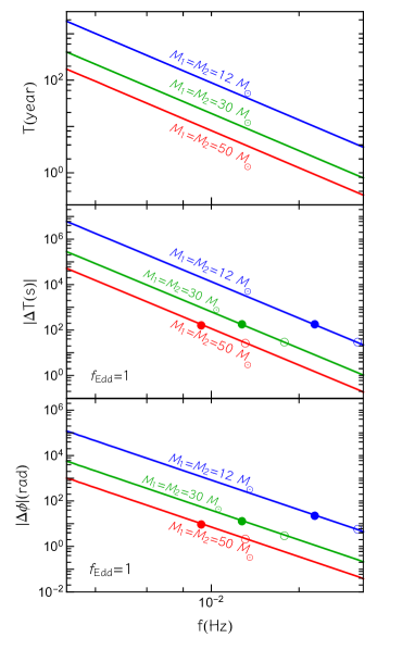
Figure 1.— Time needed to enter the band of terrestrial detectors neglecting accretion (top), time difference caused by accretion (middle), and corresponding GW phase difference (bottom), as functions of the initial GW frequency for three equal-mass SOBHBs. We choose $f_{\rm Edd}=1$ as a reference, since the time and phase differences scale linearly with $f_{\rm Edd}$. The full (empty) circles mark the points corresponding to $T=10\,{\rm yr}$ ($T=4\,{\rm yr}$). The systems to the right of the full (empty) circles therefore have $T<10\,{\rm yr}$ ($T<4\,{\rm yr}$).

3. Measuring accretion effects for SOBHBs and IMBHBs

In order to quantify the ability of multiband SOBHB detections and standalone IMBHB observations to constrain the accretion model, we perform two analyses: (i) A simple Fisher matrix analysis to explore the whole parameter space, and (ii) a more refined Monte Carlo Markov Chain (MCMC) analysis for the best candidate events. Note that the Fisher matrix analysis is only valid for large signal-to-noise ratios (SNRs) (Vallisneri, 2008). Therefore, we expect it to provide only qualitatively correct results for SOBHBs in the LISA band (for which the SNR is at most $15-20$ in the most optimistic cases, see below). Nevertheless, we expect the Fisher matrix analysis to be accurate for the IMBHBs we consider, for which ${\rm SNR}={\cal O}(100)$.

In both the Fisher and MCMC analyses we only account for the contribution due to accretion in the GW phase, and neglect the subleading contribution to the amplitude. Since accretion is important at low frequency, high-order PN terms (including the spin) should be irrelevant for our analysis, but we include them for completeness and to estimate possible correlations.

For simplicity, in the Fisher analysis we also neglect the motion of the antenna during the observation. This is instead included in the MCMC analysis, in order to estimate the ability to localize the source in the sky and measure the accretion rate at the same time.

Finally, we consider two situations: one (referred to as LISA+Earth) in which we simulate a multiband SOBHB detection (LISA combined with a ground-based interferometer) and another (referred to as LISA-only) in which we simulate a standalone (either SOBHB or IMBHB) detection by LISA. In the LISA+Earth case, to simulate a multiband detection one can follow two options: combine statistically the noise curves of LISA with that of a given ground-based detector or, alternatively (but less rigorously), assume that the merger time can be computed independently by the ground-based detector, so that the dimension of the parameter space of the analysis is effectively reduced. In the Fisher analysis, we follow the latter, simpler approach, and we therefore effectively remove the merger time from the template parameters in the LISA+Earth case. In the MCMC analysis we keep $t_{c}$ as a free parameter, restricting it by using a narrow prior. In all cases we adopt the LISA noise curve reported by Audley et al. (2017), whose high frequency part is based on a single link optical measurement system noise of 10 pm/$\sqrt{\mbox{Hz}}$.

3.1. Fisher analysis and event rates for SOBHBs

In the Fisher analysis we adopt a TaylorF2 template approximant for spinning binaries up to $3.5$PN order (Droz et al., 1999), with the addition of the leading-order accretion term presented in Eq. (2). Therefore, our GW template for the Fisher analysis has seven parameters (masses, merger time and phase, the two dimensionless spins $\chi_{1,2}$, besides the Eddington accretion ratio $f_{\rm Edd}$).

Given a waveform template $h(\vec{\zeta},f)$ in the frequency domain and a set of waveform parameters $\vec{\zeta}$, the error associated with the measurement of parameter $\zeta^{a}$ (with all other parameters marginalized upon) is $\sigma_{a}=\sqrt{\Sigma^{aa}}$, where the covariance matrix $\Sigma^{ab}$ is given by the inverse of the Fisher matrix, $\Gamma_{ab}=\left(\partial_{\zeta^{a}}h|\partial_{\zeta^{b}}h\right)_{\vec{\zeta}=\vec{\zeta}_{0}}$. Here, $\vec{\zeta}_{0}$ are the injected values of the parameters, and the inner product is defined by

$$(g|h)=4\,{\rm Re}\int_{f_{\rm 0}}^{f_{\rm max}}df\,\frac{\tilde{h}(f)\tilde{g}^{\star}(f)}{S_{h}(f)}\ ,$$ (4)

where $S_{h}(f)$ is the detector noise spectral density.

While the number (and the very existence) of IMBHBs in the LISA band is very uncertain, our Fisher-matrix analysis, coupled with simulated astrophysical populations calibrated to the LIGO/Virgo data, can easily provide estimates of the number of SOBHBs detectable by LISA for which accretion can be measured. The intrinsic number of SOBHBs merging per (detector-frame) unit time and (source-frame) masses is given by (Hartwig et al., 2016)

$$\frac{\mathrm{d}\dot{N}}{\mathrm{d}m_{1}\mathrm{d}m_{2}}=\int\mathrm{d}z\,R\frac{\mathrm{d}t}{\mathrm{d}z}\frac{\mathrm{d}^{2}p}{\mathrm{d}m_{1}\mathrm{d}m_{2}}4\pi d_{C}^{2},$$ (5)

where $d_{C}$ is the comoving distance, $R=53.2\,\text{Gpc}^{-3}\text{yr}^{-1}$ is the best estimate for the intrisic merger rate measured by the first and second LIGO/Virgo runs (Abbott et al., 2019), the probability distribution function for the source-frame masses – ${\mathrm{d}^{2}p}/{\mathrm{d}m_{1}\mathrm{d}m_{2}}$ – is given by “model B” of Abbott et al. (2019), while

$$\frac{\mathrm{d}t}{\mathrm{d}z}=\frac{1}{H_{0}(1+z)\sqrt{\Omega_{m}(1+z)^{3}+\Omega_{\Lambda}}}$$

is computed using our fiducial cosmology $H_{0}=67.9\,\text{km}/\text{s}/\text{Mpc}$, $\Omega_{m}=0.306$, $\Omega_{\Lambda}=0.694$ (Ade et al., 2016). In order to obtain synthetic astrophysical catalogues of merging as well as inspiraling sources, we use Eq. (5) to simulate mergers in a period much longer than the LISA mission duration, by assuming a uniformly distributed merger time $t_{c}$. The latter can be easily converted into the initial GW frequency $f_{0}=[5/(256\,t_{c})]^{3/8}\mathcal{M}^{-5/8}/\pi$, where $f_{0}$, $t_{c}$, and the chirp mass $\mathcal{M}$ must be computed in the same (detector- or source-) frame.

We constrain the comoving distance in the range $d_{C}\leq 2\,{\rm Gpc}$ and the initial source frame GW frequency in the range $f_{0}\in[4\,{\rm mHz},10\,{\rm Hz}]$. For the chosen mass model we generate $20$ realizations, and for each realization we consider two LISA mission durations ($4$ or $10$ yr), for a total of $40$ catalogues.

In the LISA-only case for SOBHBs, we assume that a single event within the catalogue is detected if either of the following conditions occurs (Moore, Gerosa and Klein, 2019; Tamanini et al., 2019)

$$t_{c}<100\,{\rm yr}\text{ and SNR} \geq 15,\text{ or}$$

$$t_{c}>100\,{\rm yr}\text{ and SNR} \geq 10\,,$$

where the latter SNR threshold is lower because binaries with long merger times are accurately described by Newtonian waveforms in the LISA band (Mangiagli et al., 2019) and can be therefore detected by a different search strategy (Tamanini et al., 2019), akin e.g. to the one used for white-dwarf binaries.

In the LISA+Earth case, the SNR threshold is lower for events that can be detected on Earth (Moore, Gerosa and Klein, 2019; Tamanini et al., 2019)

$$t_{c}<10\,{\rm yr}\text{ and SNR} \geq 9.5\,.$$ (6)

These events would indeed be detected through an archival search following their ground-based detection.

3.2. MCMC with sky localization and antenna motion

For the MCMC analysis we adopt the PhenomD template (Husa et al., 2016; Khan et al., 2016) with the inclusion of the phase term due to accretion. In this case we also account for the motion of the antenna during the observation. More specifically, the standard part of the GW template is the same as in Tamanini et al. (2019) and contains five additional parameters besides those adopted for the Fisher matrix analysis: two angles identifying the source position with respect to the detector ($\phi$,$\theta$), the GW polarization ($\psi$), the inclination of the system ($\iota$), and the luminosity distance ($d_{L}$).

In the LISA-only scenario we use $f_{0}$ as sampling parameter and assume a flat prior for it. In the LISA+Earth scenario we use $t_{c}$ with a Gaussian prior centered around the true value with width $\sigma_{t_{c}}=10^{-3}\,{\rm s}$ which models the fact that $t_{c}$ can be measured with great precision in this scenario. For IMBHBs, we consider a single LISA-only scenario.

Table 1Number of detectable SOBHB events for various configurations. “All” stands for the total number of detectable events, whereas $100\%$, $50\%$, and $10\%$ stand for the number of events for which $f_{\rm Edd}$ is measured with a relative error of $100\%$, $50\%$, and $10\%$, respectively, according to the Fisher analysis. All numbers are averaged over $20$ catalogues and presented with $1\,\sigma$ errors. Super-Eddington accretion will be detectable for a good fraction of multiband events if the LISA mission duration is 10 years.

	LISA+Earth					LISA-only
Duration	All	$f_{\rm Edd}$	100%	50%	10%	All	$f_{\rm Edd}$	100%	50%	10%
4 yr	88 $\pm$ 8	1	0.1 $\pm$ 0.2	0	0	77 $\pm$ 8	1	0	0	0
		10	4.1 $\pm$ 2.3	1.7 $\pm$ 1.2	0.1 $\pm$ 0.2		10	1.6 $\pm$ 1.4	0.6 $\pm$ 0.6	0
10 yr	207 $\pm$ 11	1	5.2 $\pm$ 1.9	1.1 $\pm$ 1.2	0.1 $\pm$ 0.2	182 $\pm$ 10	1	1.5 $\pm$ 1.2	0.4 $\pm$ 0.7	0
		10	36 $\pm$ 4	32 $\pm$ 3	5.2 $\pm$ 1.9		10	11 $\pm$ 3	9.5 $\pm$ 2.7	1.5 $\pm$ 1.2

When including the source location, different realizations of the angles for the same astrophysical system yield different SNRs. This affects the precision within which one can recover the parameters of the source, including the sky position itself and $f_{\rm Edd}$. In order to cross-check results obtained with our Fisher matrix analysis and to quantify this variability, we select from the catalogue an astrophysical system for which the accretion parameter can be measured precisely through the Fisher matrix approach, and draw three different realizations of ($\phi$, $\theta$, $\psi$, $\iota$) yielding a low SNR $\sim 9$, a medium SNR $\sim 15$, and a high SNR $\sim 20$, respectively. The medium SNR system is chosen so that its SNR is close to the value obtained by averaging over the angles.

For IMBHBs, we consider two systems (see details in the next section): one merging in the LIGO/Virgo band, and one with higher masses, merging at lower frequencies. We choose the inital frequency so that both systems merge in $10\,{\rm yr}$, the longest possible LISA mission duration.

For each of these systems we perform a full Bayesian analysis (see Appendix B). We simulate GW data $d(f)$ as it would be measured by LISA, computing the response of the detector (accounting for the constellation’s motion) by following Marsat and Baker (2018). We work in the zero noise approximation in order to speed up the computation. Adding noise to the GW signal should not affect the parameter estimation drastically, leading mostly to a displacement in the maximum of the parameter distribution (Rodriguez et al., 2014).

We perform two different analyses: in the first one we generate data with a non-zero value for $f_{\rm Edd}$ and include it as a free parameter in the Bayesian analysis, in order to estimate with what precision it can be recovered. In the second case, data are also generated with a non-zero value of $f_{\rm Edd}$, but when doing the analysis we set $f_{\rm Edd}=0$ in the templates, in order to measure the bias in the parameter estimation. In all cases, the posterior distribution is computed using Bayes’ theorem. Additional details are given in Appendix B.

4. Results

4.1. Event rates for SOBHBs

For the simulated astrophysical populations we first use a Fisher matrix analysis to quantify the possibility to measure $f_{\rm Edd}$ at a given precision. Table 1 shows the average number of detected SOBHBs, and the number of SOBHBs for which $f_{\rm Edd}$ can be measured within a given precision. The results are obtained by averaging the Fisher matrix over sky position and source inclination (while neglecting, as already mentioned, the LISA constellation’s motion), for different injected values of $f_{\rm Edd}$. Our results for the total number of detected events are consistent with Tamanini et al. (2019); Sesana (2016).

In particular, for the LISA+Earth case and a $10\,{\rm yr}$ mission, super-Eddington accretion $f_{\rm Edd}\approx 10$ can be measured within $50\%$ precision in about $15\%$ of the total detectable events ($\approx 200$), while a measurement within $10\%$ is only possible in $\sim 2\%$ of the events. Note that the statistical errors scale approximately linearly with $f_{\rm Edd}$. Therefore, when injecting a lower accretion rate the number of events for which accretion is measurable is significantly smaller. For example, $f_{\rm Edd}=1$ is marginally detectable in $\lesssim 1$ event in the most optimistic scenario, whereas smaller values of the accretion rates are not measurable.

As expected, a multiband observation improves the measurements of a negative-PN term, including the -4PN term due to accretion: the event rates for the LISA-only case are thus smaller by a factor of a few relative to the LISA+Earth case.

4.2. Measuring accretion and sky localization

For our MCMC analysis we select one representative SOBHB system from our synthetic astrophysical catalogues, and choose two optimistic IMBHB systems on the basis of a Fisher matrix analysis spannning the parameter space, i.e. the errors on $f_{\rm Edd}$ provided by the chosen IMBHBs are roughly the smallest throughout the parameter space. In more detail, the systems that we consider are

• A SOBHB with $m_{1}=42.1\ M_{\odot}$, $m_{2}=39.8\ M_{\odot}$, $\chi_{1}=0.008$, $\chi_{2}=0.44$, at a distance $d_{L}=416\ {\rm Mpc}$;

• An IMBHB with $m_{1}=315\ M_{\odot}$, $m_{2}=284\ M_{\odot}$, $\chi_{1}=0.9$, $\chi_{2}=0.85$, referred to as “light IMBHB”;

• Another IMBHB with $m_{1}=1000\ M_{\odot}$, $m_{2}=900\ M_{\odot}$, $\chi_{1}=0.9$, $\chi_{2}=0.85$, referred to as “heavy IMBHB”.

For all three sources we set $t_{c}\approx 10$ yr. We study the IMBHB systems at two different redshifts, $z=0.1$ and $z=0.5$, in order to estimate up to what distance the presence of accretion in the binary would be detectable. The IMBHBs’ masses are in the source frame and are kept fixed when the redshift is changed.

For each realization of the angles $(\theta,\phi,\iota,\psi)$, we compute and sample the posterior distribution as explained in Appendix B. As expected, the precision of the parameter measurements increases with the SNR. We find that the accretion parameter is strongly correlated with the intrinsic parameters of the source ($\mathcal{M}$, $\mu/M$, $f_{0}$, $\chi_{s}$, $\chi_{a}$), where $\chi_{s}$ and $\chi_{a}$ are defined in Appendix B.

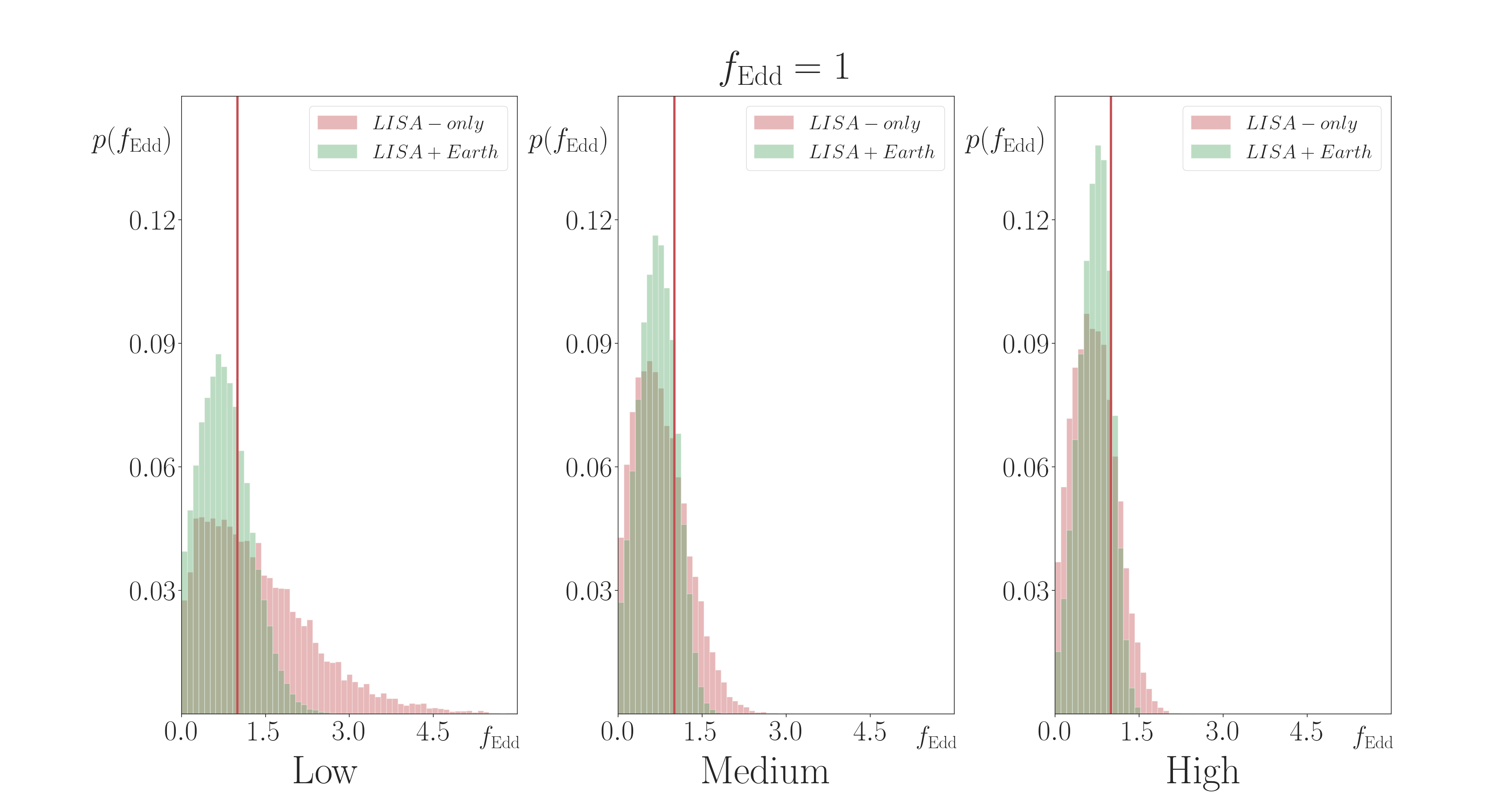
Figure 2.— Marginalized distributions of $f_{\rm Edd}$ for the considered SOBHB for various realizations of the angles, and in the scenarios LISA+Earth (green) and LISA-only (red). Red lines indicate the injected value of the accretion rate, $f_{\rm Edd}=1$. In the LISA+Earth scenario and for higher SNR the marginalized distribution is strongly peaked but still consistent with $f_{Edd}=0$.

In Fig. 2 we show the marginalized distributions of $f_{\rm Edd}$ for the chosen SOBHB system, for various SNRs and for an injected value of $f_{\rm Edd}=1$.

For the high and the medium SNR cases, already in the LISA-only scenario the posteriors indicate the presence of accretion. The marginalized distribution for $f_{\rm Edd}$ can be compared with those obtained when constraining modifications of GR (some of which affect the vacuum waveform in a similar fashion as accretion, i.e. at negative PN orders) in the parameterized post Einsteinian framework (Yunes and Pretorius, 2009). In that case, as discussed in an upcoming paper (Toubiana, Marsat, Babak and Barausse, 2020), the marginalized distribution of the non GR-parameters is mostly flat up to a threshold (representing the upper bound that can be placed on the parameters under scrutiny), and then goes to $0$. In contrast, we see in Fig. 2 that for high and medium SNR in the LISA-only scenario, the distribution peaks at some nonvanishing value, indicating the presence of a non-zero modification to the vacuum waveform.

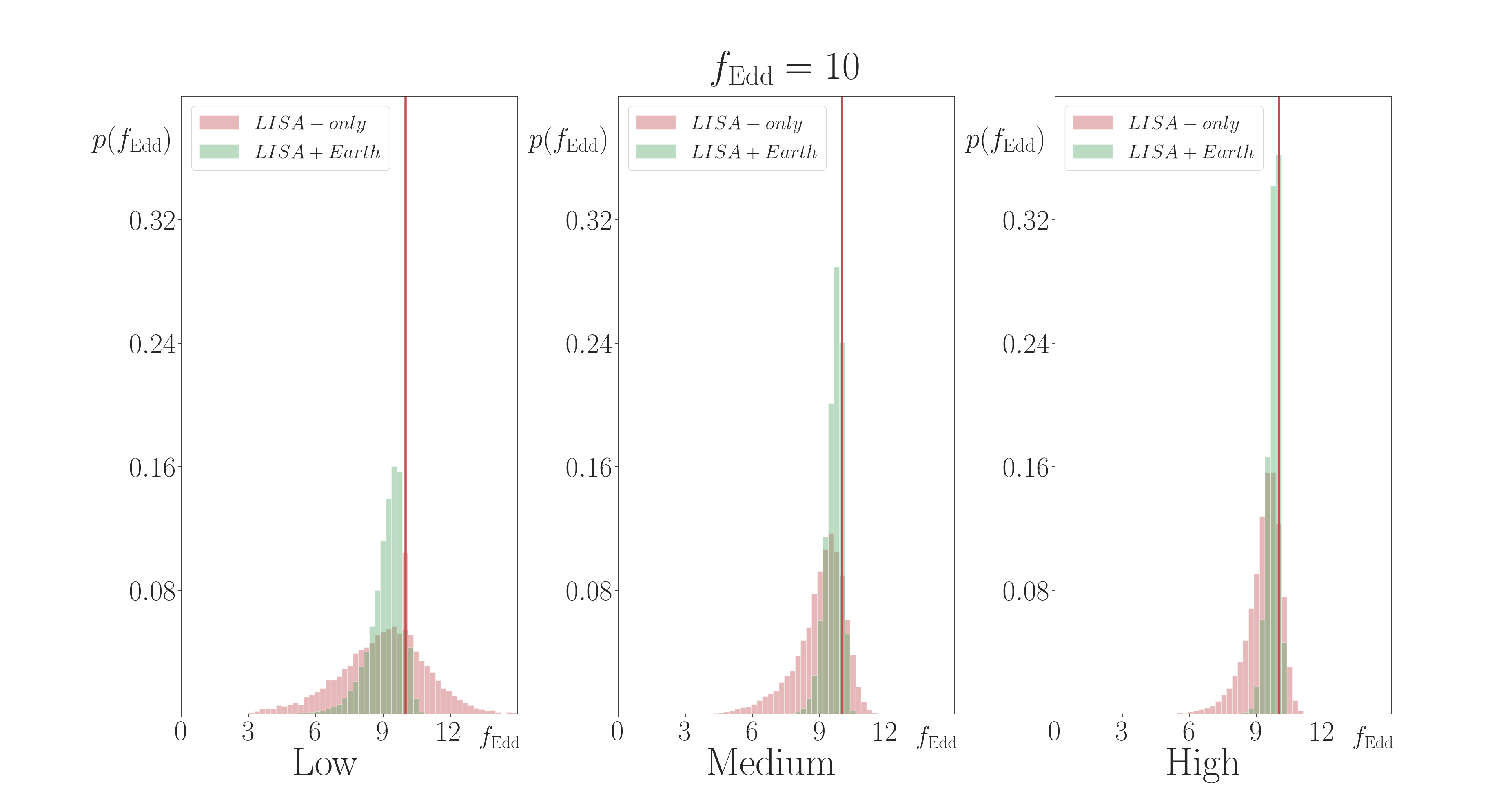
Figure 3.— Same as Fig. 2 but for an injected value of $f_{\rm Edd}=10$. Accretion is detected in all scenarios and for any angle realization.

In Fig. 3 we show the same as in Fig. 2, but for an injected value of $f_{\rm Edd}=10$. This high accretion rate can be detected more easily even in the low SNR case and in the LISA-only scenario, since in this case $f_{\rm Edd}=0$ is outside the support of the distribution. Thus, for super-Eddington accreting binaries in the LISA band, there is a concrete chance to detect the effect of high rates of accretion on the waveform for most SOBHB events.

In Table 2 we show the recovered $68\%$ confidence intervals (CI) and median values for $f_{\rm Edd}$ and the sky localization ($\Delta\Omega$). In the $f_{\rm Edd}=1$ case, since the distribution is leaning against the boundary of the prior (see Fig. 2) we define the $68\%$ CI for $f_{\rm Edd}$ by taking the lower $68\%$ values. Instead, in the $f_{\rm Edd}=10$ case, the interval is centered around the median values. The marginalized distributions for $\Delta\Omega$ are approximately Gaussian and are centered around the injected value. Thus, we define the solid angle as (Cutler, 1998):

$$\Delta\Omega=2\pi\sqrt{(\Sigma^{\phi,\phi})(\Sigma^{\cos(\theta),\cos(\theta)})-(\Sigma^{\phi,\cos(\theta)})^{2}}\,.$$ (7)

We show the same quantities for our IMBHB events in Table 3. There, in the case $f_{\rm Edd}=1$, we define the $68\%$ CI for $f_{\rm Edd}$ centered on the median, and in the case $f_{\rm Edd}=0.1$ we define it by taking the lower $68\%$ values. In all cases considered here, the error on the sky localization is much smaller than the nomimal field of view of future X-ray and radio missions, potentially allowing for the detection of electromagnetic counterparts. We will discuss this possibility in Sec. 4.3.

	$f_{\rm Edd}^{\rm injected}=1$		$f_{\rm Edd}^{\rm injected}=10$
	$f_{\rm Edd}$	$\Delta\Omega$ (${\rm deg}^{2}$)	$f_{\rm Edd}$	$\Delta\Omega$ (${\rm deg}^{2}$)
High SNR	$0.68_{-0.68}^{+0.02}$	$0.14$	$9.46_{-0.83}^{+0.53}$	$0.14$
Medium SNR	$0.70_{-0.70}^{+0.25}$	$0.06$	$9.23_{-1.23}^{+0.77}$	$0.06$
Low SNR	$1.18_{-1.18}^{+0.50}$	$0.33$	$8.82_{-2.96}^{+1.85}$	$0.34$
Fisher matrix	$1.00^{+1.20}_{-1.20}$	–	$10.00^{+1.20}_{-1.20}$	–

Table 2 Recovered $68\%$ CI on the accretion parameter $f_{\rm Edd}$ and on the sky localization $\Delta\Omega$ for SOBHBs and for various realizations in the LISA+Earth scenario. The last row gives the statistical error estimated with a Fisher-matrix analysis. The presence of accretion should be detected for super-Eddington accreting systems. The error on the sky position is always within the field of view of Athena and SKA, allowing (potentially) for electromagnetic followup.

	$f_{\rm Edd}^{\rm injected}=0.1$		$f_{\rm Edd}^{\rm injected}=1$
	$f_{\rm Edd}$	$\Delta\Omega$ (${\rm deg}^{2}$)	$f_{\rm Edd}$	$\Delta\Omega$ (${\rm deg}^{2}$)
Light IMBHB	$0.14_{-0.14}^{+0.04}$	$0.01$	$1.05_{-0.11}^{+0.10}$	$0.01$
Heavy IMBHB	$0.17_{-0.17}^{+0.05}$	$0.007$	$1.04_{-0.27}^{+0.15}$	$0.006$
Fisher matrix	$0.10_{-0.38}^{+0.38}$	–	$1.00_{-0.38}^{+0.38}$	–

Table 3 Recovered $68\%$ CI on the accretion parameter $f_{\rm Edd}$ and on the sky localization $\Delta\Omega$ for the IMBHBs considered in this work, at redshift $z=0.1$. The statistical error estimated with our Fisher-matrix analysis is similar for the two IMBHBs. The presence of accretion should be detected for Eddington accreting systems. As for SOBHBs, the error on the sky position is always within the field of view of Athena and SKA.

While overall in qualitative agreement, the differences between Fisher-matrix and MCMC results could be due to the effect of the priors, to the non-Gaussianity of the posterior distribution, to the treatment of the angles, and/or to the finite SNR of the sources considered. Nonetheless, the predicted errors on $f_{\rm Edd}$ are of the same order of magnitude in both treatments, confirming the main conclusions we drew for SOBHBs using the Fisher analysis.

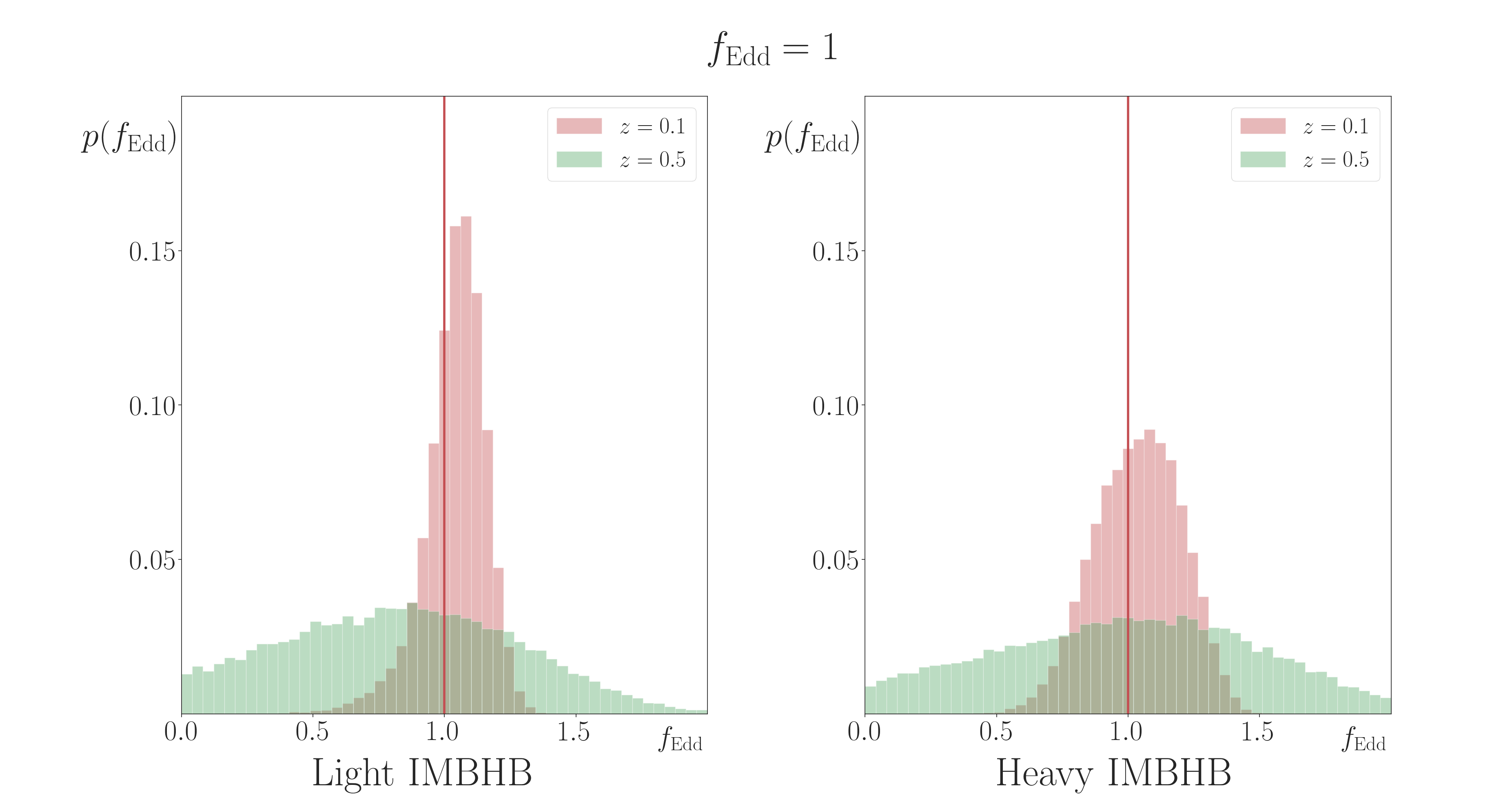
Figure 4.— Marginalized distributions of $f_{\rm Edd}$ for our two IMBHB systems at redshifts $z=0.1$ (red) and $z=0.5$ (green) for an injected value of $f_{\rm Edd}=1$. Accretion can be measured in both systems at $z=0.1$, but not at higher redshift.

In Fig. 4 we compare how well can we recover $f_{\rm Edd}$ for IMBHBs at different redshifts, for injected $f_{\rm Edd}=1$. If the system is too far, the distribution tends to be flat and the effect of accretion is hardly noticeable. This is because of the lower SNR, but also because the detector-frame mass becomes larger at higher redshift, speeding up the evolution of the system and thus providing less information on negative PN-order modifications.

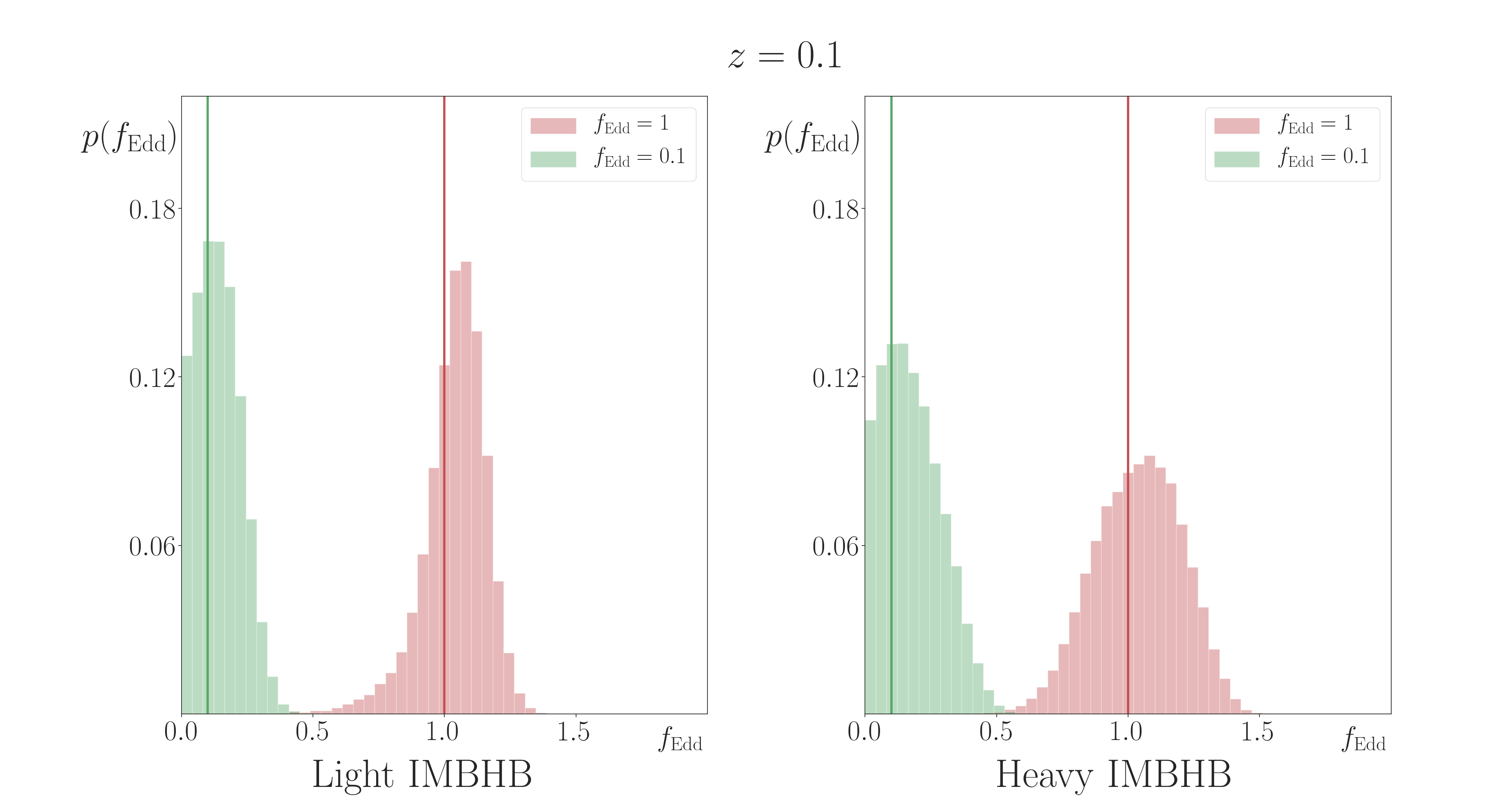
Figure 5.— Marginalized distributions of $f_{\rm Edd}$ for our two IMBHB sources for injected values of $f_{\rm Edd}=0.1$ (green) and $f_{\rm Edd}=1$ (red) at $z=0.1$. Accretion at this redshift needs to be approximately Eddington-level or stronger to be measured.

Finally in Fig. 5 we show how well can we recover $f_{\rm Edd}$ in IMBHBs for an injected values of $f_{\rm Edd}=0.1$ at $z=0.1$. As in the case of SOBHBs commented above, the marginalized distribution is compatible with $f_{\rm Edd}=0$, but the presence of a clear peak at $f_{\rm Edd}\neq 0$ favours the presence of accretion.

4.2.1 Estimating biases

The above results indicate that if accretion is present it could lead to a measurable change in the GW signal. Thus, if accretion is not taken into account, the estimation of other source parameters could be significantly biased. Since $f_{\rm Edd}$ correlates mostly with the intrinsic parameters of the source, the latter should be the most affected.

For SOBHBs in the LISA-only scenario, we find that in the three cases (high, medium, and low SNR), the signal can be recovered by an effectual template with $f_{\rm Edd}=0$, i.e., we find a maximum for the posterior distribution which, in the worst cases, can be incompatible with the injected real value. The SNR of this effectual template is very similar to the injection’s SNR (${\rm SNR}_{\rm inj}-{\rm SNR}_{\rm eff}\lesssim 0.7$), and could thus trigger a detection. The bias in the parameter estimation and the relative drop in SNR is higher for lower SNR systems and for higher injected accretion rates. The effectual template, in particular, has a higher chirp mass and a higher mass ratio, while the initial frequency is shifted towards higher values. In Figs. 6 and 7 we show how this impacts the estimate of the masses and time to coalescence for two representative values, $f_{\rm Edd}=1$ and $f_{\rm Edd}=10$. In both cases, we compare to the recovered distribution of masses for vacuum GR.

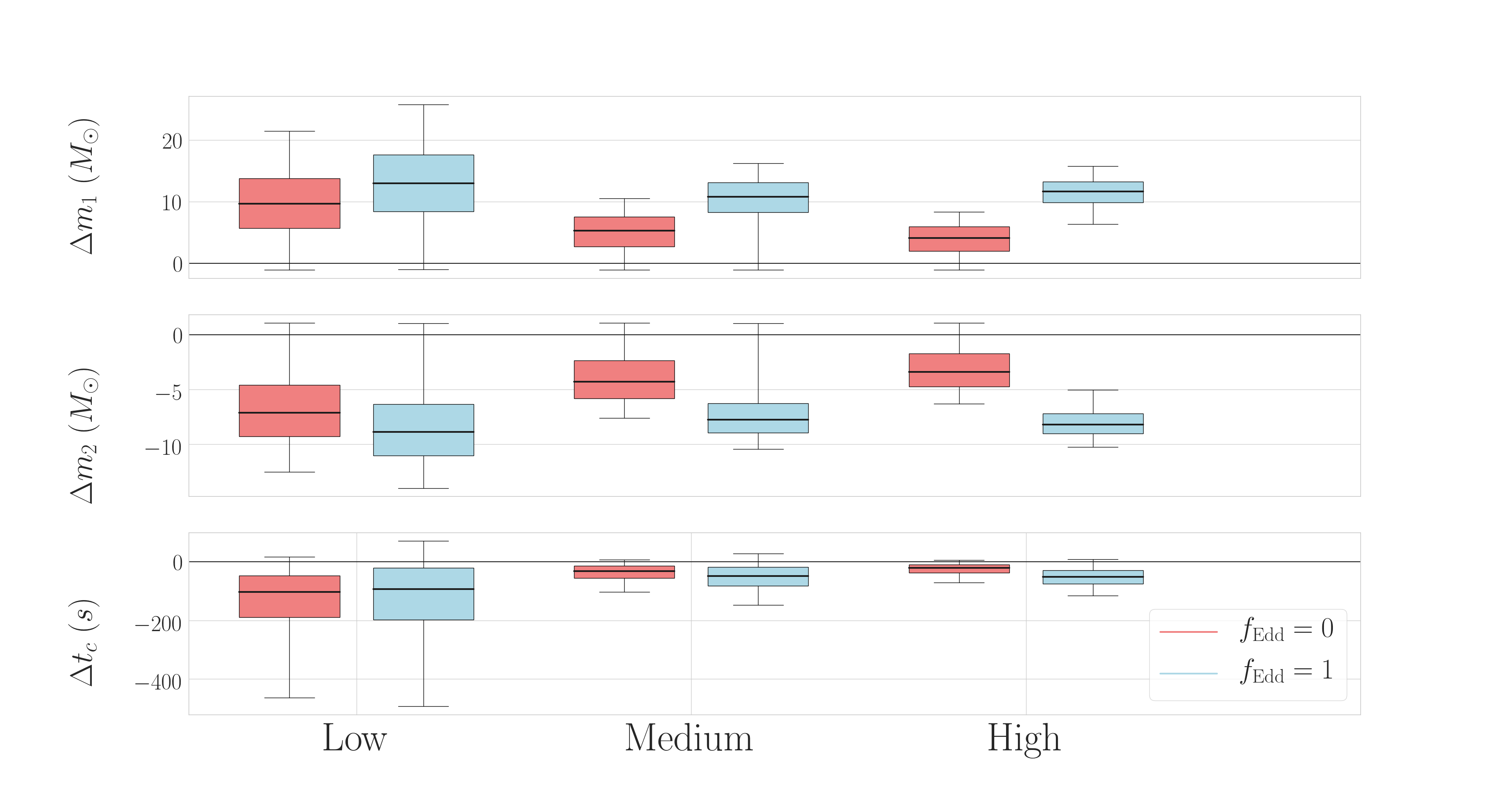
Figure 6.— Bias in the SOBH binary masses and time to coalescence induced by ignoring the corrections due to accretion when $f_{\rm Edd}=1$, for various angle realizations in the LISA-only scenario (blue) compared to the displacement found in vacuum systems. Boxes and whiskers delimit the $50\%$ CI and the $90\%$ CI, respectively, and both are centered around the median, indicated by lines inside the boxes. For this level of accretion bias is not significant, even for the high SNR realization.

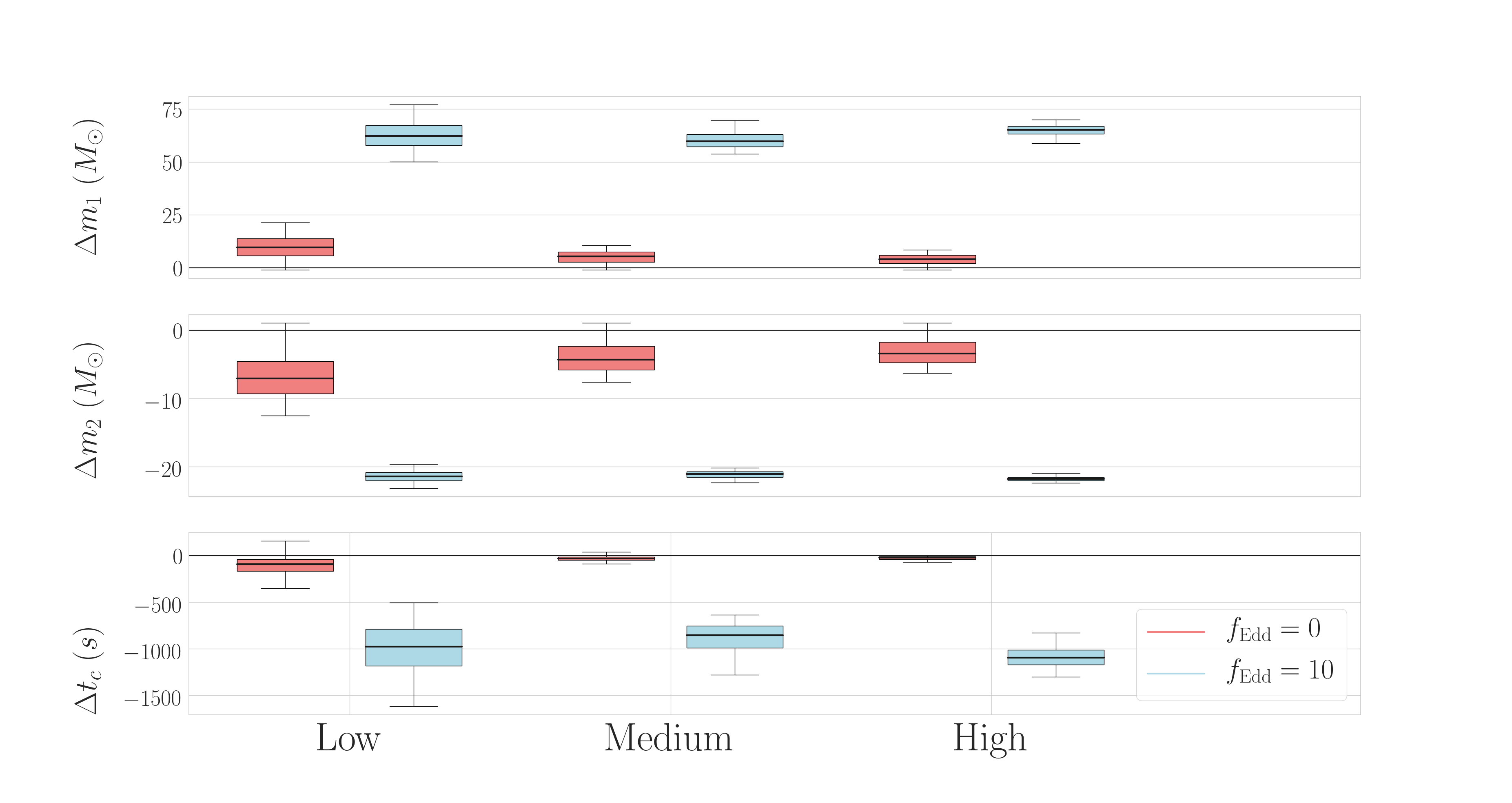
Figure 7.— Same as in Fig. 6 but comparing $f_{\rm Edd}=0$ with $f_{\rm Edd}=10$. Bias here is significant for all SNR realizations.

The mass of the primary black hole is shifted toward higher values, whereas the secondary mass gets lower. As a result, the time to coalescence is underestimated. For super-Eddington accretion, this shift in time to coalescence is at the level of tens of seconds. A multi-band observation could then help identify a bias due to accretion in the parameter estimation, since ground-based detectors would measure very precisely the time to coalescence when the signal enters in their band (Sesana, 2016).

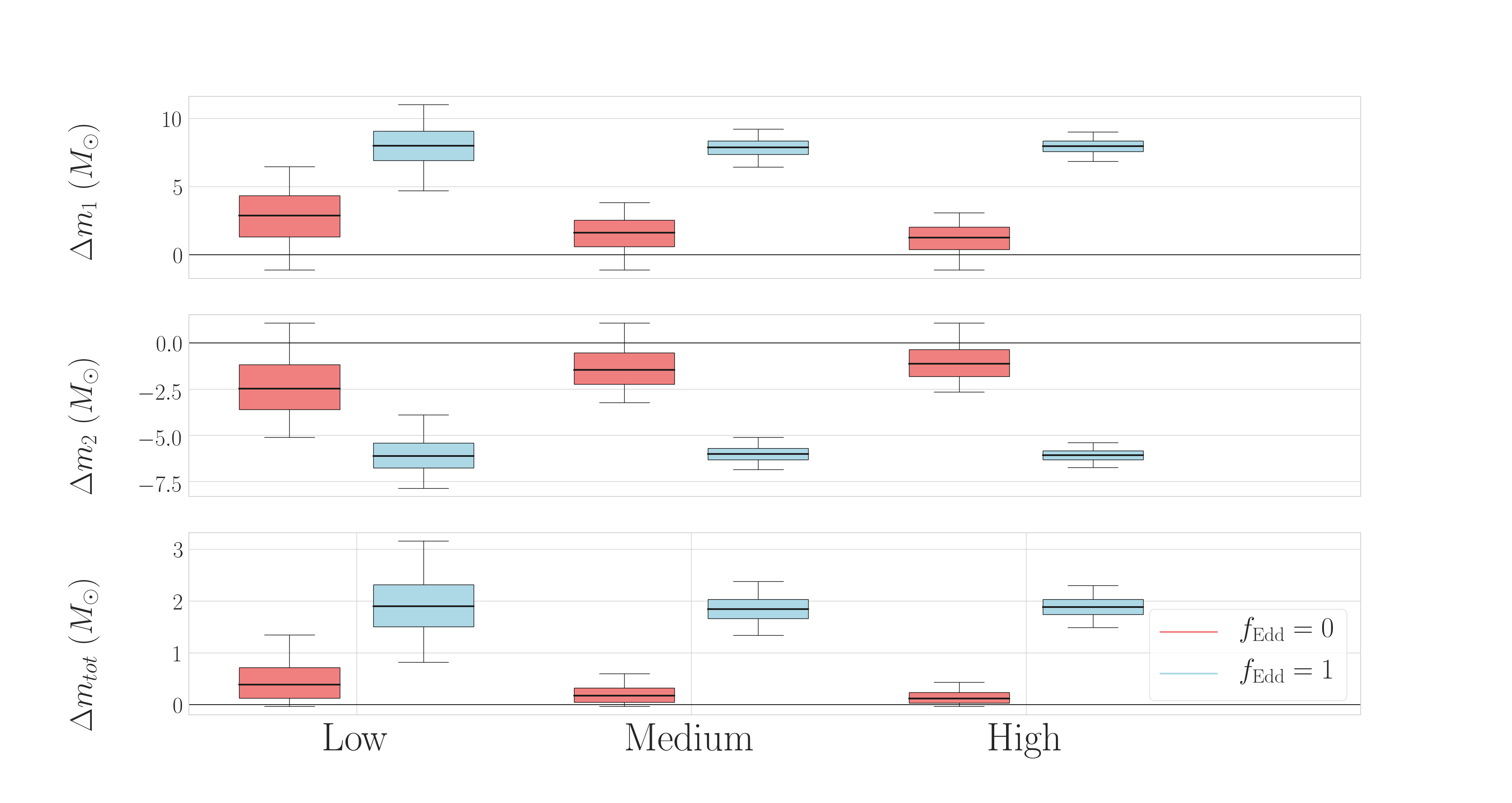
Figure 8.— Same as in Fig. 6 but for the LISA+Earth scenario. We show $m_{tot}$ rather of $t_{c}$, the latter being fixed by the narrow prior in this scenario. Bias in the masses can still be significant for medium and high SNR realizations, despite the constraint provided by ground based detectors.

In order to estimate this possibility, we repeat the above analysis in the LISA+Earth scenario. In this case the time to coalescence is constrained to within $1\,{\rm ms}$ from its true value, so no bias in $t_{c}$ is possible. Nevertheless, signals can still be recovered by an effectual template, although with a larger mismatch from the true signal. In Fig. 8 we show the difference between the recovered masses and total mass and the injected values. More in general, ground based detectors should be largely insensitive to these low frequency terms, as discussed in Carson and Yagi (2019b). In this forecast study, the projected constraint on -4PN terms with the planned third generation detector Cosmic Explorer is ten orders of magnitude worse than the projected constraint with LISA. We thus expect that observations with ground based detectors should not be biased by omitting -4PN terms. Therefore, for values of $f_{\rm Edd}$ for which the LISA parameter estimation is significantly biased, the posterior distributions obtained with LISA and with ground based detectors might not even be compatible, which would hint at an unmodelled effect.

It is noteworthy that for the SOBHB events the sky localization is barely affected by accretion and remains excellent, as the distribution remains a Gaussian centered around the injected values with errors similar to the ones shown in Table 2. In the case of IMBHBs, on the other hand, there is also a bias in the sky localization, i.e. the injected value may lie outside the $90\%$ CI. This is due to the very small errors in sky position, and in fact the the true localization is very close to the recovered one, within $0.05\,{\rm deg}^{2}$. Therefore, for most realistic purposes the sky localization is satisfactorily recovered.

Since we did not consider any modification to the GW amplitude, there is no strong correlation between $f_{\rm Edd}$ and the luminosity distance $d_{L}$. Thus, when fixing $f_{\rm Edd}=0$ as we did here, there is no bias on the estimation of $d_{L}$, contrary to the Fisher-matrix analysis in Tamanini et al. (2019), who also used waveforms modifying GR at -4PN order in phase, but included the leading-order modification to the amplitude too.

4.3. Prospects for multiband and multimessenger astronomy

According to our MCMC analysis, both SOBHBs and IMBHBs can be localized in the sky to within the fields of view of X-ray and radio instruments such as Athena WFI and SKA , $\Delta\Omega_{\rm Athena}=0.4\,{\rm deg}^{2}$, $\Delta\Omega_{\rm SKA}=0.5\,{\rm deg}^{2}$ (SKA White Paper, 2014; Meidinger, 2018). This will allow the relevant region of the sky to be covered in a single viewing, thus potentially allowing for the coincident detection of an X-ray and/or radio counterpart to strongly-accreting black hole binaries. Even if the sky localization was biased, as might be the case for IMBHBs, we estimated that the true position would still fall inside the field of view of the instruments. In the following, we compute the X-ray and radio emission of the binaries, and estimate the necessary integration time for detection by a single instrument viewing.

We start by estimating the X-ray flux. For this purpose, we assume that the accretion process has radiative efficiency $\eta=0.1$ (which is good approximation at $f_{\rm Edd}<1$), and that only a fraction $\eta_{X}=0.1$ of the EM radiation is emitted in X-rays (“bolometric correction”). We find the X-ray flux from a single accreting black hole to be

$$F_{X}\simeq 1\times 10^{-13}f_{\rm Edd}\,\Big{(}\frac{M}{M_{\odot}}\Big{)}\Big{(}\frac{{\rm Mpc}}{d_{L}}\Big{)}^{2}\,{\rm erg}\,{\rm cm}^{-2}\,{\rm s}^{-1}\,.$$ (8)

This should be compared with the flux sensitivity of the Athena WFI for a given integration time, $T_{\rm int}$. Following McGee, Sesana and Vecchio (2018), Athena’s flux sensitivity for a $5\sigma$ detection is

$$F_{X}^{\rm Athena}=1\times 10^{-15}\left(\frac{10^{3}\,{\rm s}}{T_{\rm int}}\right)^{1/2}\,{\rm erg}\,{\rm cm}^{-2}\,{\rm s}^{-1}\,.$$ (9)

The minimum integration time for a binary where only one black hole is emitting is then given by

$$T_{\rm int}\simeq 8\times 10^{-2}\,f_{\rm Edd}^{-2}\,\left(\frac{d_{L}}{{\rm Mpc}}\right)^{4}\,\left(\frac{M_{\odot}}{M}\right)^{2}\,{\rm s}\,.$$ (10)

Note that if the two black holes have similar mass and are both accreting, the cumulative flux is given by twice the value in Eq. (8) and therefore the minimum integration time is one fourth of that in Eq. (10).

For the best-candidate SOBHB event in our synthetic astrophysical catalogues, the required exposure time is $T_{\rm int}\gtrsim 1\times 10^{6}\,f_{\rm Edd}^{-2}\,{\rm s}$. Thus, even if we were to assume $f_{\rm Edd}\approx 1$, the integration time would have to be of several days. Assuming super-Eddington accretion $f_{\rm Edd}>1$ is unlikely to help as the radiative efficiency is expected to be considerably lower than our assumed $\eta=0.1$, i.e. the bolometric luminosity is not expected to significantly exceed the Eddington luminosity (Shakura and Sunyaev, 1973; Poutanen et al., 2007; Sadowski, 2011). Moreover, as previously discussed, high accretion rates in SOBHBs likely require environments with large gas densities, whose optical thickness further reduces the chances of an EM detection. For the considered IMBHB systems, the required integration time is between $24$ and $2$ hours for Eddington-level accretion, for the light and heavy systems, respectively. This estimate suggests that detection of X-ray counterparts will be possible for highly-accreting IMBHBs.

A binary system in external magnetic fields may also launch dual radio jets, which get amplified by the coalescence (Palenzuela, Lehner and Liebling, 2010) relative to similar jets observed in isolated black holes (Steiner, McClintock and Narayan, 2012). See also Moesta et al. (2012) for simulations that yield $\sim$100 times larger (though less collimated) fluxes than Palenzuela, Lehner and Liebling (2010). Assuming a fiducial value $\eta=0.1$ for the radiative efficiency of the process and $\eta_{\rm radio}=0.1$ for the fraction of emission in the radio band, the corresponding peak flux is (Palenzuela, Lehner and Liebling, 2010; Tamanini et al., 2016)

$$F_{\rm flare}\simeq 2\times 10^{-13}\,f_{\rm Edd}\,q^{2}\,\left(\frac{D_{L}}{{\rm Mpc}}\right)^{-2}\left(\frac{M}{M_{\odot}}\right)\\ \times{\rm erg}\,{\rm cm}^{-2}\,{\rm s}^{-1}\,,$$ (11)

where $q\leq 1$ is the mass ratio. The flare flux can then be compared with the SKA-mid sensitivity in the phase 1 implementation. The required sensitivity at frequency $\nu_{\rm SKA}$ for SKA,

$$F_{\rm SKA}=5\times 10^{-16}\left(\frac{10^{-2}\,{\rm s}}{T_{\rm obs}}\right)^{1/2}\left(\frac{\nu_{\rm SKA}}{{\rm GHz}}\right)\,{\rm erg}\,{\rm cm}^{-2}\,{\rm s}^{-1}\,,$$ (12)

is reached for an observation time $T_{\rm obs}\sim 10^{-2}\,{\rm s}$ for our best SOBHB event. The observation time should be smaller than the duration of the merger (i.e., the duration of the flare) for the system (Steiner, McClintock and Narayan, 2012), $T_{\rm flare}\sim 25\,\,\frac{M}{100M_{\odot}}$ ms. This condition is not satisfied for SOBHBs. There is however the concrete possibility to detect a signal in the radio band for IMBHBs, for which for the light and heavy systems $T_{\rm obs}\approx 40$ – $4\ {\rm ms}<T_{\rm flare}$. The performance of full SKA should improve by an order of magnitude with respect to Eq. (12), reducing the required integration time by a factor $100$.

5. Discussion

SOBHBs and IMBHBs provide the opportunity to measure the effect of accretion, which might affect the GW waveform at low frequencies. Our analysis suggests that a multiband detection with LISA and a ground-based detector will be able to measure the accretion parameter of strongly-accreting SOBHBs to within $50\%$ precision for a few events. For these systems, neglecting accretion in the waveform template might lead to biases in the recovered binary parameters. These biases can be alleviated by an accurate measurement of the time of coalescence by a ground-base detector.

IMBHBs in the local universe, if they exist as LISA sources, might also provide very accurate measurements of the accretion rate. Overall, for these systems the effect of accretion should be included in the waveform to avoid bias in the intrinsic binary parameters.

Finally, accretion does not affect sky localization by LISA for SOBHBs and it impacts that of IMBHBs only mildly. In both cases, the measurement errors are typically well within Athena’s and SKA fields of view. Furthermore, the X-ray flux expected from strongly-accreting binaries is comparable with Athena’s sensitivity and is well above the sensitivity of future missions such as Lynx (The Lynx Mission Concept Study Interim Report, 2018). Likewise, in the case of jets the radio signal from IMBHBs could be detectable by SKA. Our analysis shows that the simultaneous operation of Athena/SKA and LISA would therefore provide the thrilling opportunity to detect the EM counterpart of highly accreting black hole binaries.

Appendix A Accretion term in the GW waveform

An accreting binary can be described by a Hamiltonian $H(\bm{q},\bm{p})$, where the masses vary adiabatically. As shown for instance in Landau and Lifshitz (1960) and Sivardière (1988), the action variables $I_{q}=\oint p{\rm d}q/(2\pi)$ are adiabatic invariants. In our case, working in polar coordinates $r,\phi$ and in the center of mass frame, we then have that $I_{\phi}=p_{\phi}$ and $I_{r}=\oint p_{r}{\rm d}r/(2\pi)$ are conserved under accretion. The latter implies that circular orbits remain circular under accretion, while the former is equivalent to the conservation of the orbital angular momentum under accretion.

Then, to leading order, angular momentum is only lost through GWs (Peters, 1964),

$$\dot{L}_{GW}=-\frac{32\,m_{1}^{2}\,m_{2}^{2}\,M^{1/2}}{5\,r^{7/2}}=-\frac{32}{5}\mu^{2}\omega^{7/3}\,M^{4/3}\,.$$ (A1)

Defining the reduced angular momentum $\tilde{L}_{z}=L_{z}/\mu M=\sqrt{r/M}$, the evolution of the binary can be obtained through

$$\dot{\tilde{L}}_{z}=\frac{\dot{L}_{GW}}{\mu M}\,.$$ (A2)

Integrating Eq. (A2), we find the evolution of the orbital frequency,

$$\omega_{\rm GW}(t)=\left(\omega_{0}^{-8/3}-\frac{256}{5}M^{2/3}\,\mu\,t\right)^{-3/8}\,,$$ (A3)

where $\omega_{0}=\pi f_{0}$ is the initial orbital frequency. The time as a function of the orbital frequency is found inverting this expression,

$$t_{\rm GW}(\omega)=t_{c}-\frac{5}{256\,\mu\,M^{2/3}\,\omega^{8/3}}\,,$$ (A4)

where $t_{c}$ is the merger time in the Newtonian approximation. In the stationary-phase approximation, the GW phase reads (Cutler and Flanagan, 1994; Maggiore, 2008)

$$\phi_{\rm GW}(f)=2\pi ft_{c}+\phi_{c}-2\int_{t}^{t_{c}}\omega_{\rm GW}(t^{\prime})dt^{\prime}=2\pi ft_{c}+\phi_{c}+\frac{3}{4}\left(8\pi\mathcal{M}f\right)^{-5/3}\,,$$

where $\phi_{c}$ is the phase at merger.

We shall now compare these known results with what happens in the presence of mass accretion. We assume that the binary is surrounded by gas and that both bodies are accreting mass at a same fraction of the Eddington rate,

$$m_{i}(t)=m_{i,0}\,e^{f_{\rm Edd}\,t/\tau}\,,$$ (A5)

where $\tau=4.5\times 10^{7}\,{\rm yr}$ is known as the Salpeter time scale and $m_{i,0}$ is the initial mass of the $i$-th body. When this time dependence is taken into account in the expression for the angular momentum, Eq. (A2) acquires an extra term:

$$\dot{\tilde{L}}_{z}=\frac{\dot{L}_{GW}}{\mu M}-\tilde{L}_{z}\frac{\dot{(\mu M)}}{\mu M}\,.$$ (A6)

In this equation, all masses should be considered time dependent, except the ones appearing in the angular momentum radiated by GWs. This is because accretion cannot be considered adiabatic compared to GW emission.
Accretion will in general be accompanied by a drag force $\vec{F}_{{\rm drag}}$ due to the fact that the accreted material carries some angular momentum. This effect can be quantified as

$$\vec{F}_{{\rm drag},i}=\dot{m}_{i}(\vec{v}_{\rm gas}-\vec{v}_{i})\,.$$ (A7)

for each mass, where $\vec{v}_{i}$ is the velocity of the $i$-th body. For simplicity we parametrize this effect with a constant factor $\xi$, fixed by the relative velocity between the gas and the perturber (Barausse and Rezzolla, 2008; Barausse, Cardoso and Pani, 2014),

$$\vec{F}_{{\rm drag},i}\simeq-\xi\,\dot{m}_{i}\vec{v}_{i}\quad\rightarrow\quad\dot{L}_{\rm drag}=-\xi\,\dot{\mu}\,r^{2}\omega\,.$$ (A8)

Note that the parameter $\xi$ can be positive (drag) or negative (pull, see e.g. Gruzinov, Levin and Matzner, 2019). At leading order in $f_{\rm Edd}\xi$, the term $\dot{L}_{\rm drag}/\mu M$ should be added to the right-hand side of Eq. (A6) to take the effect of the drag into account.

We can now solve the total angular momentum variation equation for the orbital frequency,

$$\omega_{\rm acc}(t)=5^{3/8}e^{f_{\text{Edd}}\frac{(3\xi+5)}{\tau}t}\left(5\,\omega_{0}^{-8/3}-\frac{768\,\mu_{0}\,M_{0}^{2/3}\tau\left(e^{f_{\text{Edd}}\frac{(24\xi+35)}{3\tau}t}-1\right)}{(24\xi+35)f_{\text{Edd}}}\right)^{-3/8},$$ (A9)

where $M_{0}$ and $\mu_{0}$ are the initial values of the total and reduced mass, respectively. This expression cannot be inverted exactly to find $t=t(\omega)$. We therefore use a perturbative expansion valid when the accretion correction is small, i.e. we assume $t_{\rm acc}(\omega)=t_{\rm GW}(\omega)+f_{\rm Edd}\,t^{(1)}_{\rm acc}(\omega)+\mathcal{O}(f_{\rm Edd}^{2})$. We verified this to be an excellent approximation in all realistic situations, including when $f_{\rm Edd}\sim 1-100$. This is because the dimensionless parameter always appears in the combination $f_{Edd}\cdot t/\tau$, which is always small for the evolution times scales that we consider.

In terms of the GW frequency, we find

$$t^{(1)}_{\rm acc}(f)=-\frac{25\left(\pi^{16/3}f^{16/3}(24\,\xi+35)-3\pi^{16/3}f_{0}^{16/3}(8\,\xi+15)+10\,\pi^{16/3}\left(ff_{0}\right){}^{8/3}\right)}{393216\,\pi^{32/3}\left(ff_{0}\right){}^{16/3}\mu_{0}^{2}\,M_{0}^{4/3}\tau}.$$ (A10)

Finally, we can compute the contribution of accretion to the GW phase in the stationary phase approximation, $h\sim|h|\,e^{i\phi}$, at first order in perturbation theory, i.e. $\phi\simeq\phi_{\rm GW}+\phi_{\rm acc}=2\pi f\left(t_{\rm GW}+f_{\rm Edd}\,t^{(1)}_{\rm acc}\right)-\int_{0}^{t_{\rm GW}+f_{\rm Edd}\,t^{(1)}_{\rm acc}}2\,\omega_{\rm acc}\,{\rm d}t$. We find, again as a function of the GW frequency,

$$\phi_{\rm acc}= -f_{{\rm Edd}}\,(8\,\xi+15)\,\frac{75\,\mathcal{M}_{0}}{851968\,\tau}\,\left(\pi f\mathcal{M}_{0}\right){}^{-13/3}+f_{{\rm Edd}}\,\frac{25}{32768\,\pi^{8/3}\,f_{0}^{8/3}\,\mathcal{M}_{0}^{5/3}\,\tau}\,\left(\pi f\mathcal{M}_{0}\right){}^{-5/3}$$

$$+f_{{\rm Edd}}\,(3\,\xi+4)\,\frac{25}{19968\,\pi^{13/3}\,f_{0}^{13/3}\,\mathcal{M}_{0}^{10/3}\tau}-f_{{\rm Edd}}\,(24\,\xi+35)\,\frac{25}{196608\,\pi^{16/3}\,f_{0}^{16/3}\,\mathcal{M}_{0}^{13/3}\tau}\,\left(\pi f\mathcal{M}_{0}\right)\,.$$ (A11)

In the expression above, the terms linear in frequency and independent of frequency can be reabsorbed in the definition of the time to coalescence $t_{c}$ and the phase at coalescence $\phi_{c}$, respectively. Eq. (A) tells us that the GW signal will be dominated by the effect of accretion if the frequency is sufficiently low. By comparing the size of the leading order phase term (0PN) in the vacuum waveform and the -4PN term induced by accretion, we find that accretion is the dominant effect at frequencies below

$$f_{\rm acc}\simeq\frac{1}{\pi}\left(\frac{25}{3}\frac{45}{6656}\frac{f_{\rm Edd}}{\tau}\right)^{3/8}\mathcal{M}^{-5/8}\,.$$ (A12)

While in Eq. A we show all the terms of the expansion, we have verified that the -4PN term dominates. The inclusion of the 0PN term changes the results of the main text by less than $1\%$. This is expected since most of the binary evolution in the LISA band takes place at large separation/low frequencies.

In the analysis presented in the main text we discarded the terms proportional to the drag coefficient $\xi$, which would add an additional parameter in our waveform and require proper modeling of the distribution of the gas and its velocity around the black holes. From the functional form of Eq. (A) we can see that neglecting the drag does not affect the frequency dependence of the GW phase, while it might affect the size of the effect. However, $f_{\rm Edd}$ and $\xi$ enter the two leading terms in Eq. (A) in different combinations, which would help disentangle the two effects. Indeed we checked that for generic values of $\xi$ the time and phase shifts presented in Fig. 1 do not vary dramatically.

Appendix B Details on the MCMC analysis

Using Bayes’ theorem we compute the posterior distribution for $\zeta$, the multidimensional vector parameterizing a waveform template $h$ given observed data $d$:

$$p(\zeta|d)=\frac{p(d|\zeta)p(\zeta)}{p(d)}$$ (B1)

For the prior, $p(\zeta)$, we assume a flat distribution in $m_{1}$ and $m_{2}$ with $m_{1}\geq m_{2}\geq 3M_{\odot}$, flat in spin magnitude between $-1$ and $1$, volume uniform for the source localization and flat in the source orientation, its polarization and its initial phase. In the LISA-only scenario we assume a flat prior in initial frequency and in the LISA+Earth scenario we use instead a Gaussian prior centered around the true value of $t_{c}$ of width $\sigma_{t_{c}}=10^{-3}{\rm s}$. Assuming Gaussian noise, the likelihood is given by $p(d|\zeta)=e^{-\frac{1}{2}(d-h|d-h)}$ where parenthesis denote the inner product defined by: $(h_{1}|h_{2})=4\mathfrak{Re}\left(\int\frac{\tilde{h_{1}}(f)\ \tilde{h_{2}}^{*}(f)}{S_{n}(f)}{\rm d}f\right)$. In the denominator, $S_{n}(f)$ is the detector power spectral density, indicating the level of noise at a given frequency.
To sample the posterior distribution we use a Metropolis Hashtings Markov Chain Monte Carlo (MHMCMC) (Karandikar, 2006; Understanding the Metropolis-Hastings Algorithm, 1995) algorithm that we designed for this problem. More details will be given in an upcoming publication (Marsat, Baker and Dal Canton, 2020; Toubiana, Marsat, Babak, Baker and Dal Canton, 2020). The basic idea of the algorithm is to explore the parameter space through a Markov chain generated with a symmetric proposal $\pi$, $\pi(\zeta_{1},\zeta_{2})=\pi(\zeta_{2},\zeta_{1})$. Starting from a point $\zeta_{0}$, we accept the proposed point $\zeta_{p}$ with a probability given by the ratio of the posterior distribution, $\frac{p(\zeta_{p})}{p(\zeta_{0})}$. By doing so we accumulate samples representing the distribution. In order to increase the sampling efficiency, we parametrize the waveforms with parameters for which – based on the PN expressions (Buonanno, Cook and Pretorius, 2007; Buonanno et al., 2009) – we believe the posterior distribution is simpler. We take $\zeta=(\mathcal{M},\mu/M,f_{0},\chi_{s},\chi_{a},f_{\rm Edd},\phi,\sin(\theta),\psi,\phi_{0},\cos(\iota),\log 10_{d_{L}})$ in the LISA-only scenario. In the LISA+Earth scenario we use $t_{c}$ instead of $f_{0}$. Here $\chi_{s}$ is the symmetric combination of spins

$$\chi_{s}=\frac{m_{1}\chi_{1}+m_{2}\chi_{2}}{m_{1}+m_{2}}\,,$$ (B2)

while $\chi_{a}$ is the corresponding antisymmetric combination,

$$\chi_{a}=\frac{m_{1}\chi_{1}-m_{2}\chi_{2}}{m_{1}+m_{2}}\,.$$ (B3)

For the proposal $\pi$, we use a Gaussian distribution based on Fisher matrix. To ensure we have independent samples we downsample the chain using the autocorrelation length.

To strenghten our confidence in our MHMCMC we cross-checked our results obtained with it to the ones obtained with Multinest, a public nested sampling algorithm (Feroz, Hobson and Bridges, 2009; Skilling, 2006).

References

- (1)
- Abbott et al. (2016a) Abbott, B. P. et al. 2016a. “Astrophysical Implications of the Binary Black-Hole Merger GW150914.” Astrophys. J. 818(2):L22.
- Abbott et al. (2016b) Abbott, B. P. et al. 2016b. “Localization and broadband follow-up of the gravitational-wave transient GW150914.” Astrophys. J. 826(1):L13.
- Abbott et al. (2019) Abbott, B. P. et al. 2019. “Binary Black Hole Population Properties Inferred from the First and Second Observing Runs of Advanced LIGO and Advanced Virgo.” The Astrophysical Journal 882(2):L24.
- Ade et al. (2016) Ade, P. A. R. et al. 2016. “Planck 2015 results. XIII. Cosmological parameters.” Astron. Astrophys. 594:A13.
- Antonini and Perets (2012) Antonini, F. and H. B. Perets. 2012. “Secular Evolution of Compact Binaries near Massive Black Holes: Gravitational Wave Sources and Other Exotica.” ApJ 757:27.
- Atakan Gurkan, Freitag and Rasio (2004) Atakan Gurkan, M., Marc Freitag and Frederic A. Rasio. 2004. “Formation of massive black holes in dense star clusters. I. mass segregation and core collapse.” Astrophys. J. 604:632–652.
- Audley et al. (2017) Audley, Heather et al. 2017. “Laser Interferometer Space Antenna.”.
- Barausse and Rezzolla (2008) Barausse, Enrico and Luciano Rezzolla. 2008. “The Influence of the hydrodynamic drag from an accretion torus on extreme mass-ratio inspirals.” Phys. Rev. D77:104027.
- Barausse, Yunes and Chamberlain (2016) Barausse, Enrico, Nicolás Yunes and Katie Chamberlain. 2016. “Theory-Agnostic Constraints on Black-Hole Dipole Radiation with Multiband Gravitational-Wave Astrophysics.” Phys. Rev. Lett. 116(24):241104.
- Barausse, Cardoso and Pani (2014) Barausse, Enrico, Vitor Cardoso and Paolo Pani. 2014. “Can environmental effects spoil precision gravitational-wave astrophysics?” Phys. Rev. D89(10):104059.
- Barausse, Cardoso and Pani (2015) Barausse, Enrico, Vitor Cardoso and Paolo Pani. 2015. “Environmental Effects for Gravitational-wave Astrophysics.” J. Phys. Conf. Ser. 610(1):012044.
- Buonanno et al. (2009) Buonanno, Alessandra, Bala Iyer, Evan Ochsner, Yi Pan and B. S. Sathyaprakash. 2009. “Comparison of post-Newtonian templates for compact binary inspiral signals in gravitational-wave detectors.” Phys. Rev. D80:084043.
- Buonanno, Cook and Pretorius (2007) Buonanno, Alessandra, Gregory B. Cook and Frans Pretorius. 2007. “Inspiral, merger and ring-down of equal-mass black-hole binaries.” Phys. Rev. D75:124018.
- Cardoso and Maselli (2019) Cardoso, Vitor and Andrea Maselli. 2019. “Constraints on the astrophysical environment of binaries with gravitational-wave observations.”.
- Carson and Yagi (2019a) Carson, Zack and Kent Yagi. 2019a. “Multi-band gravitational wave tests of general relativity.”.
- Carson and Yagi (2019b) Carson, Zack and Kent Yagi. 2019b. “Parameterized and inspiral-merger-ringdown consistency tests of gravity with multi-band gravitational wave observations.”.
- Charles and Coe (2003) Charles, P. A. and M. J. Coe. 2003. “Optical, ultraviolet and infrared observations of X-ray binaries.” arXiv e-prints pp. astro–ph/0308020.
- Chen and Shen (2019) Chen, Xian and Zhe-Feng Shen. 2019. “Retrieving the True Masses of Gravitational-wave Sources.” MDPI Proc. 17(1):4.
- Cutler (1998) Cutler, Curt. 1998. “Angular resolution of the LISA gravitational wave detector.” Phys. Rev. D57:7089–7102.
-
Cutler and Flanagan (1994)
Cutler, Curt and Éanna E. Flanagan. 1994.
“Gravitational waves from merging compact binaries: How accurately
can one extract the binary’s parameters from the inspiral waveform?” Phys. Rev. D 49:2658–2697.
https://link.aps.org/doi/10.1103/PhysRevD.49.2658 -
Droz et al. (1999)
Droz, Serge, Daniel J. Knapp, Eric Poisson and Benjamin J. Owen. 1999.
“Gravitational waves from inspiraling compact binaries: Validity of
the stationary-phase approximation to the Fourier transform.” Physical
Review D 59(12).
http://dx.doi.org/10.1103/PhysRevD.59.124016 - Ducci et al. (2013) Ducci, L., M. Sasaki, F. Haberl and W. Pietsch. 2013. “X-ray source population study of the starburst galaxy M83 with XMM-Newton.” Astron. Astrophys. 553:A7.
- Feroz, Hobson and Bridges (2009) Feroz, F., M. P. Hobson and M. Bridges. 2009. “MultiNest: an efficient and robust Bayesian inference tool for cosmology and particle physics.” Mon. Not. Roy. Astron. Soc. 398:1601–1614.
- Flanagan and Hughes (1998) Flanagan, Eanna E. and Scott A. Hughes. 1998. “Measuring gravitational waves from binary black hole coalescences: 2. The Waves’ information and its extraction, with and without templates.” Phys. Rev. D57:4566–4587.
- Frank, King and Raine (2002) Frank, J., A. King and D. J. Raine. 2002. Accretion Power in Astrophysics: Third Edition.
- Gnocchi et al. (2019) Gnocchi, Giuseppe, Andrea Maselli, Tiziano Abdelsalhin, Nicola Giacobbo and Michela Mapelli. 2019. “Bounding Alternative Theories of Gravity with Multi-Band GW Observations.”.
- Gruzinov, Levin and Matzner (2019) Gruzinov, Andrei, Yuri Levin and Christopher D. Matzner. 2019. “Negative Dynamical Friction on compact objects moving through dense gas.”.
- Hartwig et al. (2016) Hartwig, Tilman, Marta Volonteri, Volker Bromm, Ralf S. Klessen, Enrico Barausse, Mattis Magg and Athena Stacy. 2016. “Gravitational Waves from the Remnants of the First Stars.” Mon. Not. Roy. Astron. Soc. 460(1):L74–L78.
- Holgado and Ricker (2019) Holgado, A. Miguel and Paul M. Ricker. 2019. “Gravitational Radiation from Close Binaries with Time-Varying Masses.”.
- Husa et al. (2016) Husa, Sascha, Sebastian Khan, Mark Hannam, Michael Pürrer, Frank Ohme, Xisco Jiménez Forteza and Alejandro Bohé. 2016. “Frequency-domain gravitational waves from nonprecessing black-hole binaries. I. New numerical waveforms and anatomy of the signal.” Phys. Rev. D93(4):044006.
-
Karandikar (2006)
Karandikar, Rajeeva L. 2006.
“On the Markov Chain Monte Carlo (MCMC) method.” Sadhana
31(2):81–104.
https://doi.org/10.1007/BF02719775 -
Khan et al. (2016)
Khan, Sebastian, Sascha Husa, Mark Hannam, Frank Ohme, Michael Pürrer,
Xisco Jiménez Forteza and Alejandro Bohé. 2016.
“Frequency-domain gravitational waves from nonprecessing black-hole
binaries. II. A phenomenological model for the advanced detector era.” Phys. Rev. D 93:044007.
https://link.aps.org/doi/10.1103/PhysRevD.93.044007 - Kinugawa et al. (2014) Kinugawa, Tomoya, Kohei Inayoshi, Kenta Hotokezaka, Daisuke Nakauchi and Takashi Nakamura. 2014. “Possible Indirect Confirmation of the Existence of Pop III Massive Stars by Gravitational Wave.” Mon. Not. Roy. Astron. Soc. 442(4):2963–2992.
- Landau and Lifshitz (1960) Landau, L. D. and E. M Lifshitz. 1960. Course on theoretical Physics: Mechanics. Wiley.
- Latif and Ferrara (2016) Latif, Muhammad A. and Andrea Ferrara. 2016. “Formation of supermassive black hole seeds.” Publ. Astron. Soc. Austral. 33:e051.
- Leigh, Sills and Boker (2013) Leigh, Nathan W. C., Alison Sills and Torsten Boker. 2013. “Modifying two-body relaxation in N-body systems by gas accretion.” Mon. Not. Roy. Astron. Soc. 433:1958.
- Lindblom, Owen and Brown (2008) Lindblom, Lee, Benjamin J. Owen and Duncan A. Brown. 2008. “Model Waveform Accuracy Standards for Gravitational Wave Data Analysis.” Phys. Rev. D78:124020.
- Madau and Rees (2001) Madau, Piero and Martin J. Rees. 2001. “Massive black holes as Population III remnants.” Astrophys. J. 551:L27–L30.
- Maggiore (2008) Maggiore, M. 2008. Gravitational Waves: Volume 1: Theory and Experiments. Oxford University Press.
- Mangiagli et al. (2019) Mangiagli, Alberto, Antoine Klein, Alberto Sesana, Enrico Barausse and Monica Colpi. 2019. “Post-Newtonian phase accuracy requirements for stellar black hole binaries with LISA.” Phys. Rev. D99(6):064056.
- Mapelli (2016) Mapelli, Michela. 2016. “Massive black hole binaries from runaway collisions: the impact of metallicity.” Mon. Not. Roy. Astron. Soc. 459(4):3432–3446.
- Marchant et al. (2016) Marchant, Pablo, Norbert Langer, Philipp Podsiadlowski, Thomas M. Tauris and Takashi J. Moriya. 2016. “A new route towards merging massive black holes.” Astron. Astrophys. 588:A50.
- Marsat, Baker and Dal Canton (2020) Marsat, Sylvain, John Baker and Tito Dal Canton. 2020. To appear .
- Marsat and Baker (2018) Marsat, Sylvain and John G. Baker. 2018. “Fourier-domain modulations and delays of gravitational-wave signals.”.
- McGee, Sesana and Vecchio (2018) McGee, Sean, Alberto Sesana and Alberto Vecchio. 2018. “The assembly of cosmic structure from baryons to black holes with joint gravitational-wave and X-ray observations.”.
- McKernan et al. (2018) McKernan, Barry, K. E. Saavik Ford, J. Bellovary, N. W. C. Leigh, Z. Haiman, B. Kocsis, W. Lyra, M. M. Mac Low, B. Metzger, M. O’Dowd, S. Endlich and D. J. Rosen. 2018. “Constraining Stellar-mass Black Hole Mergers in AGN Disks Detectable with LIGO.” ApJ 866(1):66.
- Meidinger (2018) Meidinger, N. 2018. “The Wide Field Imager instrument for Athena.” Contributions of the Astronomical Observatory Skalnate Pleso 48(3):498–505.
- Mezcua (2017) Mezcua, Mar. 2017. “Observational evidence for intermediate-mass black holes.” International Journal of Modern Physics D 26(11):1730021.
- Miller, Fabian and Miller (2004) Miller, J. M., A. C. Fabian and M. C. Miller. 2004. “A Comparison of Intermediate-Mass Black Hole Candidate Ultraluminous X-Ray Sources and Stellar-Mass Black Holes.” ApJ 614(2):L117–L120.
- Miller and Hamilton (2002) Miller, M. Coleman and Douglas P. Hamilton. 2002. “Production of intermediate-mass black holes in globular clusters.” Mon. Not. Roy. Astron. Soc. 330:232.
- Miller and Colbert (2004) Miller, M. Coleman and E. J. M Colbert. 2004. “Intermediate - mass black holes.” Int. J. Mod. Phys. D13:1–64.
- Moesta et al. (2012) Moesta, Philipp, Daniela Alic, Luciano Rezzolla, Olindo Zanotti and Carlos Palenzuela. 2012. “On the Detectability of Dual Jets from Binary Black Holes.” ApJ 749(2):L32.
- Moore, Gerosa and Klein (2019) Moore, Christopher J., Davide Gerosa and Antoine Klein. 2019. “Are stellar-mass black-hole binaries too quiet for LISA?” Mon. Not. Roy. Astron. Soc. 488(1):L94–L98.
- Palenzuela, Lehner and Liebling (2010) Palenzuela, Carlos, Luis Lehner and Steven L. Liebling. 2010. “Dual Jets from Binary Black Holes.” Science 329:927.
- Peters (1964) Peters, P. C. 1964. “Gravitational Radiation and the Motion of Two Point Masses.” Phys. Rev. 136:B1224–B1232.
- Portegies Zwart et al. (2004) Portegies Zwart, Simon F., Holger Baumgardt, Piet Hut, Junichiro Makino and Stephen L. W. McMillan. 2004. “The Formation of massive black holes through collision runaway in dense young star clusters.” Nature 428:724.
- Portegies Zwart and McMillan (2002) Portegies Zwart, Simon F. and Steve L. W. McMillan. 2002. “The Runaway growth of intermediate-mass black holes in dense star clusters.” Astrophys. J. 576:899–907.
- Poutanen et al. (2007) Poutanen, Juri, Sergei Fabrika, Alexey G. Butkevich and Pavel Abolmasov. 2007. “Supercritically accreting stellar mass black holes as ultraluminous X-ray sources.” Mon. Not. Roy. Astron. Soc. 377:1187–1194.
- Rodriguez et al. (2014) Rodriguez, Carl L., Benjamin Farr, Vivien Raymond, Will M. Farr, Tyson B. Littenberg, Diego Fazi and Vicky Kalogera. 2014. “Basic Parameter Estimation of Binary Neutron Star Systems by the Advanced LIGO/Virgo Network.” Astrophys. J. 784:119.
- Ryu et al. (2016) Ryu, Taeho, Takamitsu L. Tanaka, Rosalba Perna and Zoltán Haiman. 2016. “Intermediate-mass black holes from Population III remnants in the first galactic nuclei.” Mon. Not. Roy. Astron. Soc. 460(4):4122–4134.
- Sadowski (2011) Sadowski, A. 2011. “Slim accretion disks around black holes.” arXiv e-prints p. arXiv:1108.0396.
- Schneider et al. (2002) Schneider, R., A. Ferrara, P. Natarajan and K. Omukai. 2002. “First stars, very massive black holes and metals.” Astrophys. J. 571:30–39.
- Sesana (2016) Sesana, Alberto. 2016. “Prospects for Multiband Gravitational-Wave Astronomy after GW150914.” Phys. Rev. Lett. 116(23):231102.
- Shakura and Sunyaev (1973) Shakura, N. I. and R. A. Sunyaev. 1973. “Black holes in binary systems. Observational appearance.” Astron. Astrophys. 24:337–355.
- Sivardière (1988) Sivardière, Jean. 1988. “Adiabatic invariants for harmonic and Kepler motions.” European Journal of Physics 9(2):150–151.
-
SKA White Paper (2014)
SKA White Paper. 2014.
https://www.skatelescope.org/wp-content/uploads/2014/03/SKA-TEL-SKO-0000308_SKA1_System_Baseline_v2_DescriptionRev0 1-part-1-signed.pdf -
Skilling (2006)
Skilling, John. 2006.
“Nested sampling for general Bayesian computation.” Bayesian
Anal. 1(4):833–859.
https://doi.org/10.1214/06-BA127 -
Steiner, McClintock and Narayan (2012)
Steiner, James F., Jeffrey E. McClintock and Ramesh Narayan. 2012.
“Jet power and black hole spin: testing an empirical relationship
and using it to predict the spins of six black holes.” The
Astrophysical Journal 762(2):104.
http://dx.doi.org/10.1088/0004-637X/762/2/104 - Stone, Metzger and Haiman (2017) Stone, Nicholas C., Brian D. Metzger and Zoltán Haiman. 2017. “Assisted inspirals of stellar mass black holes embedded in AGN discs: solving the ‘final au problem’.” MNRAS 464(1):946–954.
- Tamanini et al. (2019) Tamanini, Nicola, Antoine Klein, Camille Bonvin, Enrico Barausse and Chiara Caprini. 2019. “The peculiar acceleration of stellar-origin black hole binaries: measurement and biases with LISA.”.
- Tamanini et al. (2016) Tamanini, Nicola, Chiara Caprini, Enrico Barausse, Alberto Sesana, Antoine Klein and Antoine Petiteau. 2016. “Science with the space-based interferometer eLISA. III: Probing the expansion of the Universe using gravitational wave standard sirens.” JCAP 1604(04):002.
- The Lynx Mission Concept Study Interim Report (2018) The Lynx Mission Concept Study Interim Report. 2018.
- Toubiana, Marsat, Babak and Barausse (2020) Toubiana, Alexandre, Sylvain Marsat, Stanislav Babak and Enrico Barausse. 2020. To appear .
- Toubiana, Marsat, Babak, Baker and Dal Canton (2020) Toubiana, Alexandre, Sylvain Marsat, Stanislav Babak, John Baker and Tito Dal Canton. 2020. To appear .
-
Understanding the Metropolis-Hastings
Algorithm (1995)
Understanding the Metropolis-Hastings Algorithm. 1995.
The American Statistician 49(4):327–335.
http://www.jstor.org/stable/2684568 - Vallisneri (2008) Vallisneri, Michele. 2008. “Use and abuse of the Fisher information matrix in the assessment of gravitational-wave parameter-estimation prospects.” Phys. Rev. D77:042001.
- Yunes and Pretorius (2009) Yunes, Nicolas and Frans Pretorius. 2009. “Fundamental Theoretical Bias in Gravitational Wave Astrophysics and the Parameterized Post-Einsteinian Framework.” Phys. Rev. D80:122003.