Encode, Shuffle, Analyze Privacy Revisited:
Formalizations and Empirical Evaluation

Abstract

Recently, a number of approaches and techniques have been introduced for reporting software statistics with strong privacy guarantees, spurred by the large-scale deployment of mechanisms such as Google’s RAPPOR [1].

Ranging from abstract algorithms to comprehensive systems, and varying in their assumptions and applicability, this work has built upon local differential privacy mechanisms, sometimes augmented by anonymity. Most recently, based on the Encode, Shuffle, Analyze (ESA) framework [2], a notable set of results has formally clarified how making reports anonymous can greatly improve privacy guarantees without loss of utility [3, 4]. Unfortunately, these results have comprised either systems with seemingly incomparable mechanisms and attack models, or formal statements that have given little guidance to practitioners.

To address this, in this work we provide a formal treatment and offer prescriptive guidelines for privacy-preserving reporting with anonymity, i.e., for deployments of “privacy amplification by shuffling.” To achieve this, we revisit the ESA framework and craft a simple, abstract model of attackers and assumptions covering it and other proposed systems of anonymity. In light of the new formal privacy bounds, we examine the limitations of sketch-based encodings and ESA mechanisms such as data-dependent crowds. However, we also demonstrate how the ESA notion of fragmentation—i.e., reporting different data aspects in separate, unlinkable messages—is essential for improving the privacy/utility tradeoff both in terms of local and central differential-privacy guarantees.

Finally, to help practitioners understand the applicability and limitations of privacy-preserving reporting, we report on a large number of empirical experiments. In these, we mostly use real-world datasets with heavy-tailed or near-flat distributions, since these pose the greatest difficulty for our techniques; in particular, we focus on data drawn from images, since it can be easily visualized in a way that highlights errors in its reconstruction. Showing the promise of the approach, and of independent interest, we also report on experiments using anonymous, privacy-preserving reporting to train high-accuracy deep neural networks on standard tasks, such as MNIST and CIFAR-10.

I Introduction

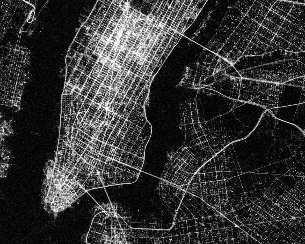
Figure 1: A differentially-private view of the NYC smartphone-location data published by the New York Times in 2018 [5]. Anonymous, randomized location reports allow high accuracy with a strong central differential privacy guarantee ($\varepsilon_{c}=0.5$) and a weaker local guarantee ($\varepsilon_{\ell^{\infty}}\approx 12$) that still provides uncertainty even if all parties collude and break report anonymity.

To guide their efforts, public health officials must sometimes gather statistics based on sensitive, private information (e.g., to survey the prevalence of vaping among middle-school children). Due to privacy concerns—or simple reluctance to admit the truth—respondents may fail to answer such surveys, or purposefully answer incorrectly, despite the societal benefits of improved public-health measures.

To remove such discouragement, and still compute accurate statistics, epidemiologists can turn to randomized response and have respondents not report their true answer, but instead report the results of random coin flips that are just biased by that true answer [6].

In computing, such randomized-response mechanisms that guarantee local differential privacy (LDP) have become a widely-deployed, best-practice means of gathering potentially-sensitive information about software and its users in a responsible manner [1, 7]. Simultaneously, many systems have been developed for anonymous communication and messaging [8, 9], many of which are designed to gather aggregate statistics with privacy [2, 10, 11, 12]. As shown in Figure 1, when combined with anonymity, LDP reports can permit high-accuracy central visibility into distributed, sensitive data (e.g., different users’ private attributes) with strong worst-case privacy guarantees that hold for even the most unlucky respondents—even when fate and other parties conspire against them. Thereby, a key dilemma can be resolved: how to usefully learn about a population’s data distribution without collecting distinct, identifiable population data into a database whose very existence forms an unbounded privacy risk, especially as it may be abused for surveillance.

I-A Statistical Reporting with Privacy, in Practice

Unfortunately, in practice, there remains little clarity on how statistical reporting should be implemented and deployed with strong privacy guarantees—especially if LDP reports are to be made anonymous [2, 3, 13, 14]. A daunting number of LDP reporting protocols have been recently proposed and formally analyzed, each using slightly different assumptions and techniques, such as strategies for randomization and encoding of binary, categorical, and other types of data [1, 15, 16, 17]. However, these protocols may not be suitable to the specifics of any given application domain, due to their different assumptions, (e.g., about adaptivity [3, 14], sketching [1, 18, 15, 16], or succinctness of communication [15, 16, 19]). Thus, these protocols may exhibit lackluster performance on real-world data distributions of limited size, even when accompanied by a formal proof of asymptotically-optimal privacy/utility tradeoffs. In particular, many of these protocols perform dimensionality-reduction using sketches whose added noise may greatly thwart visibility into the tail of distributions (as shown in the experiments of Section VII). Finally, the option of simply replicating the details of prominent LDP-reporting deployments is not very attractive, since these have been criticized both for a lack of privacy and a lack of utility [1, 2, 20].

Similarly, multiple, disparate approaches have been developed for ensuring anonymity, including some comprehensive systems that have seen wide deployment [8]. However, most of these are not well suited to gathering statistics with strong privacy, as they are focused on low-latency communication or point-to-point messaging [8, 9, 21]. The few that are well-suited to ensuring the anonymity of long-term, high-latency statistical reporting are somewhat incomparable, due to their different technical mechanisms and their varying assumptions and threat models. Whether they rely on Tor-like mixnets or trusted hardware, some proposed systems output sets of reports unlinkable to their origin [2, 13], while others output only a summary of the reports made anonymous by the use of a commutative, associative aggregation operation [10, 11]. Also, these systems’ abilities are constrained by the specifics of their construction and mechanisms (e.g., built-in sampling rates and means of multi-party cryptographic computation, as in [11]); some systems are more specific still, and focus only on certain applications, such as the maintenance of (statistical) models [12, 22]. Finally, all of these systems have slightly different threat models, e.g., with some assuming an honest-but-curious central coordinator [11] and other assuming a non-colluding, trusted set of parties [2, 10]. (Interestingly, these threat models typically exclude the risk of statistical inference, even though limiting this risk is often a primary privacy goal, as it is in this paper.) All of this tends to obscure how these anonymity systems can be best applied to learning statistics with strong privacy guarantees.

This lack of clarity is especially concerning because of recent formal results—known colloquially as “privacy amplification by shuffling” [3, 13, 14, 19]—which have fundamentally changed privacy/utility tradeoffs and forced a reconsideration of previous approaches, like those described above. These amplification results prove how central privacy guarantees can be strengthened by orders of magnitude when LDP reports can be made anonymous—i.e., unlinkable to their source—in particular, by having them get “lost in the crowd” through their shuffling or aggregate summarization with a sufficiently-large set of other reports.

The source of these privacy amplification results are efforts to formalize how LDP reporting mechanisms benefit from anonymity in the Encode, Shuffle, Analyze (ESA) framework [2]. The ESA architecture is rather abstract—placing few restrictions on specifics such as randomization schemes, report encoding, or the means of establishing anonymity—and, not surprisingly, can be a suitable foundation for implementations that aim to benefit from privacy amplification by anonymity.

I-B Practical Experiments, Primitives, and Attack Models

In this work, we revisit the specifics of the ESA framework and explore statistical reporting with strong privacy guarantees augmented by anonymity, with the goal of providing clear, practical implementation guidelines.

At the center of this paper are a set of empirical experiments, modeled on real-world monitoring tasks, that achieve different levels of privacy on a representative set of data distributions. For most of our experiments we use data distributions derived from images, which we choose because they are both representative of certain sensitive data—such as user-location data, as in Figure 1—and their reconstruction accuracy can be easily estimated, visually. Reconstructing images with strong privacy is particularly challenging since images are a naturally high-dimensional dataset with a low maximum amplitude (e.g., the per-pixel distribution of an 8-bit gray-scale image will have a luminescence bound of 255), and which can be either dense or sparse. In addition, following most previous work, we also include experiments that use a real-world, Zipfian dataset with high-amplitude heavy hitters.

The overall conclusion of this paper is that high-accuracy statistical reporting with strong, anonymity-amplified privacy guarantees can be implemented using a small set of simple primitives: (i) a new “removal” basis for the analysis of LDP reporting, (ii) one-hot encoding of categorical data, (iii) fragmenting of data and reports into multiple messages, and (iv) anonymous shuffling or aggregate sums. Although novel in combination, most of these individual primitives have been explored in previous work; the exception is our “removal LDP” report definition which can strengthen the local privacy guarantees by a factor of two. For several common statistical reporting tasks, we argue that these four primitives are difficult to improve upon, and we verify this in experiments.

Interestingly, we find that some of the more advanced primitives from the related work may offer little benefits and can, in some cases, be detrimental to privacy and utility. These include ESA’s Crowd IDs and the heterogeneous privacy levels they induce, by identifying subsets of reports, as well as—most surprisingly—the use of the sketch-based encodings like those popularized by RAPPOR [1, 16]. As we shown in experiments, while sketching will always reduce the number of sent reports, sketching may add noise that greatly exceeds that required for privacy, unless the sketch construction is fine-tuned to the target data-distribution specifics.

However, we find great benefits in the ESA concept of fragments: breaking up the information to be reported and leveraging anonymity to send multiple unlinkable reports, instead of sending the same information in just one report. As an example, using attribute fragmentation, a respondent with different attributes encoded into a long, sparse Boolean bitvector can send multiple, separately-anonymous reports for the index of each bit set in an LDP version of the bitvector. In particular, we show how privacy/utility tradeoffs can be greatly improved by applying such attribute fragmentation to LDP reports based on one-hot encodings of categorical data. Another useful form is report fragmentation, where respondents send multiple, re-randomized reports based on an LDP backstop (e.g., an underlying, permanent LDP report, like the PRR of [1]); this can allow for a more refined attack model and lower the per-report privacy risk, while maintaining a strict cap on the overall, long-term privacy loss.

Finally, we propose a simple, abstract model of threats and assumptions that abstracts away from the how shuffling is performed and assumes only that LDP report anonymization satisfy a few, clear requirements; thereby, we hope to help practitioners reason about and choose from the disparate set of anonymization systems, both current and future. The requirements of our attack model can be met using a variety of mechanisms, such as mixnets, anonymous messaging, or a variety of cryptographic multi-party mechanisms including ESA’s “blinded shuffling” [2]. Furthermore, while simple, our attack model still allows for refinements—such as efficient in-system aggregation of summaries, and gradual loss of privacy due to partial compromise or collusion—which may be necessary for practical, real-world deployments.

I-C Summary of Contributions

This paper gives clear guidelines for how practitioners can implement high-accuracy statistical reporting with strong privacy guarantees—even for difficult, high-dimensional data distributions, and as little as a few dozen respondents—and best leverage recent privacy-amplification results based on anonymity. In particular, this paper contributes the following:

1. We explain how the reports in anonymous statistical monitoring are well suited to a “removal LDP” definition of local differential privacy and how this can strengthen respondents’ local privacy guarantees by a factor of two, without compromise.

2. We give the results of numerous experiments that are representative of real-world tasks and data distributions and show that strong central privacy guarantees are compatible with high utility—even for low-amplitude and long-tail distributions—but that this requires high-epsilon LDP reports and, correspondingly, great trust in how reports are anonymized.

3. We clarify how—given the strong central privacy guarantees allowed by anonymity—the use of higher-epsilon LDP reports is almost always preferable to mechanisms, like ESA Crowd IDs, which perform data-dependent grouping of reports during anonymization.

4. We outline how privacy and utility can be maximized by having respondents use attribute fragmentation to break up their data (such as the different bits of their reports) and send as separate, unlinkable LDP reports.

5. We formally analyze how—along the lines of RAPPOR’s permanent randomized response [1]—report fragmentation can reduce the per-report privacy risk, while strictly bounding the overall, long-term privacy loss.

6. We empirically show the advantages of simple one-hot LDP report encodings and—as a warning to practitioners—empirically highlight the need to fine-tune the parameters of sketch-based encodings.

7. We provide a simple, abstract attack model that makes it easier to reason about the assumptions and specifics of anonymity mechanisms and LDP reporting schemes, and compose them into practical systems.

8. Finally, we demonstrate how anonymous LDP reports can be usefully applied to the training of benchmark deep learning models with high accuracy, with clear central privacy guarantees and minimal empirical loss of privacy.

II Definitions and Assumptions

We first lay a foundation for the remainder of this paper by defining notation, terms, and stating clear assumptions. In particular, we clarify what we mean by LDP reports, their encoding and fragmentation, as well as our model of attackers and anonymization.

II-A Local Differential Privacy and Removal vs. Replacement

Differential privacy (DP), introduced by Dwork et al. [23, 24], is a privacy definition that captures how randomized algorithms that operate on a dataset can be bounded in their sensitivity to the presence or absence of any particular data item. Differential privacy is measured as the maximum possible divergence between the output distributions of such algorithms when applied to two datasets that differ by any one record. The most common definition of this metric is based on the worst-case replacement of any dataset record:

Definition II.1 (Replacement $(\varepsilon,\delta)$-DP [25]).

A randomized algorithm $\mathcal{M}\colon\mathcal{D}^{n}\rightarrow\mathcal{S}$ satisfies replacement $(\varepsilon,\delta)$-differential privacy if for all $S\subset\mathcal{S}$ and for all $i\in[n]$ and datasets $D=(x_{1},\ldots,x_{n}),D^{\prime}=(x^{\prime}_{1},\ldots,x^{\prime}_{n})\in\mathcal{D}^{n}$ such that $x_{j}=x^{\prime}_{j}$ for all $j\neq i$ we have:

$$\mathop{\mathbf{Pr}}[\mathcal{M}(D)\in S]\leq e^{\varepsilon}\mathop{\mathbf{Pr}}[\mathcal{M}(D^{\prime})\in S]+\delta.$$

Above, as in the rest of this paper, we let $[n]$ denote the set of integers $\{1,\ldots,n\}$, $[a,b]$ denote $\{v\colon a\leq v\leq b\}$, and $(a\wedge b)$ denote $\text{max}(a,b)$. Symbols such as $x$ typically represent scalars, symbols such as $\boldsymbol{x}$ represent vectors of appropriate length. Elements of $\boldsymbol{x}$ are represented by $x_{i}$. Respectively, $\|\boldsymbol{x}\|_{1}$ and $\|\boldsymbol{x}\|_{2}$ represent $\sum|x_{i}|$ and $\sqrt{\sum x_{i}^{2}}$. Additionally, all logarithms in this paper are natural logarithms, unless the base is explicitly mentioned.

Local differential privacy (LDP) considers a distributed dataset or data collection task where an attacker is assumed to see and control the reports or records for all-but-one respondent, and where the entire transcript of all communication must satisfy differential privacy for each respondent. Commonly, LDP guarantees are achieved by having respondents communicate only randomized reports that result from applying a differentially private algorithm $\mathcal{R}$ to their data.

For any given level of privacy, there are strict limits to the utility of datasets gathered via LDP reporting. The uncertainty in each LDP report creates a “noise floor” below which no signal can be detected. This noise floor grows with the dimensionality of the reported data; therefore, compared to a Boolean question (“Do you vape?”), a high-dimensional question about location (“Where in the world are you?”) can be expected to have dramatically more noise and a correspondingly worse signal. This noise floor also grows in proportion to the square root of the number of reports; therefore, somewhat counter-intuitively, as more data is collected it will become harder to detect any fixed-magnitude signal (e.g., the global distribution of the limited, fixed set of people named Sandiego).

The algorithms used to create per-respondent LDP reports—referred to as local randomizers—must satisfy the definition of differential privacy for a dataset of size one; in particular, they may satisfy the following definition based on replacement:

Definition II.2 (Replacement LDP).

An algorithm $\mathcal{R}\colon\mathcal{D}\rightarrow\mathcal{S}$ is a replacement $(\varepsilon,\delta)$-differentially private local randomizer if for all $S\subseteq\mathcal{S}$ and for all $x,x^{\prime}\in\mathcal{D}$:

$$\mathop{\mathbf{Pr}}[\mathcal{R}(x)\in S]\leq e^{\varepsilon}\mathop{\mathbf{Pr}}[\mathcal{R}(x)\in S]+\delta.$$

However, this replacement-based LDP definition is unnecessarily conservative—at least for finding good privacy/utility tradeoffs in statistical reporting—although it has often been used in prior work, because it simplifies certain analyses.

Replacement LDP compares the presence of any respondent’s report against the counterfactual of being replaced with its worst-case alternative. For distributed monitoring, a more suitable counterfactual is one where the respondent has decided not to send any report, and thereby has removed themselves from the dataset. It is well known that replacement LDP has a differential-privacy $\varepsilon$ upper bound that for some mechanisms can be twice that of an $\varepsilon$ based on the removal of a respondent’s report. For the $\varepsilon>1$ regime that is typical in LDP applications, this factor-of-two change makes a major difference because the probability of $S$ depends exponentially on $\varepsilon$. Thus, a removal-based definition is more appropriate for our practical privacy/utility tradeoffs. Unfortunately, a removal-based LDP definition cannot be directly adopted in the local model due to a technicality: removing any report will change the support of the output distribution because the attacker is assumed to observe all communication. To avoid this, we can define removal-based differential privacy generally with respect to algorithms defined only on inputs of fixed length $n$, and from this define a corresponding local randomizer:

Definition II.3 (Generalized removal $(\varepsilon,\delta)$-DP).

A randomized algorithm $\mathcal{M}\colon\mathcal{D}^{n}\rightarrow\mathcal{S}$ satisfies removal $(\varepsilon,\delta)$-differential privacy if there exists an algorithm $\mathcal{M}^{\prime}\colon\mathcal{D}^{n}\times 2^{[n]}\rightarrow\mathcal{S}$ with the following properties:

1. for all $D\in\mathcal{D}^{n}$, $\mathcal{M}^{\prime}(D,[n])$ is identical to $\mathcal{M}(D)$;

2. for all $D\in\mathcal{D}^{n}$ and $I\subseteq[n]$, $\mathcal{M}^{\prime}(D,I)$ depends only on the elements of $D$ with indices in $I$;

3. for all $S\subset\mathcal{S}$, $D\in\mathcal{D}^{n}$ and $I,I^{\prime}\subseteq[n]$ where we have that $|I\bigtriangleup I^{\prime}|=1$:

   $$\mathop{\mathbf{Pr}}[\mathcal{M}^{\prime}(D,I)\in S]\leq e^{\varepsilon}\mathop{\mathbf{Pr}}[\mathcal{M}^{\prime}(D,I^{\prime})\in S]+\delta.$$

(Notably, this definition generalizes the more standard definition of removal-based differential privacy where $\mathcal{M}$ is defined for datasets of all sizes, by setting $\mathcal{M}^{\prime}(D,I):=\mathcal{M}((x_{i})_{i\in I})$—i.e., by defining $\mathcal{M}^{\prime}(D,I)$ to be $\mathcal{M}$ applied to the elements of $D$ with indices in $I$.)

In the distributed setting it suffices to define removal-based LDP—as follows—by combining the above definition with the use of a local randomizer whose properties satisfy Definition II.3 when restricted to datasets of size 1. (For convenience, we state this only for $\delta=0$, since extensions to $\delta>0$ and other notions of DP are straightforward.)

Definition II.4 (Removal LDP).

An algorithm $\mathcal{R}\colon\mathcal{D}\rightarrow\mathcal{S}$ is a removal $\varepsilon$-differentially private local randomizer if there exists a random variable $\mathcal{R}_{0}$ such that for all $S\subseteq\mathcal{S}$ and for all $x\in\mathcal{D}$:

$$e^{-\varepsilon}\mathop{\mathbf{Pr}}[\mathcal{R}_{0}\in S]\leq\mathop{\mathbf{Pr}}[\mathcal{R}(x)\in S]\leq e^{\varepsilon}\mathop{\mathbf{Pr}}[\mathcal{R}_{0}\in S].$$

Here $\mathcal{R}_{0}$ should be thought of as the output of the randomizer when a respondent’s data is absent. This definition is equivalent, up to a factor of two, to the replacement version of the definitions. To distinguish between these two notions we will always explicitly state “removal differential privacy” but often omit “replacement” to refer to the more common notion.

II-B Attributes, Encodings, and Fragments of Reports

There are various means by which LDP reports can be crafted from a respondent’s data record, $\boldsymbol{x}\in\mathcal{D}$ in a domain $\mathcal{D}$, using a local randomizer $\mathcal{R}$. This paper considers three specific LDP report constructions, that stem from the ESA framework [2]—report encoding, attribute fragmentation, and report fragmentation—each of which provides a lever for controlling different aspects of the utility/privacy tradeoffs.

Encodings: Given a data record $\boldsymbol{x}$, depending on its domain $\mathcal{D}$, the type of encoding can have a strong impact on the utility of a differentially private algorithm. Concretely, consider a setting where the domain $\mathcal{D}$ is a dictionary of elements (e.g., words in a language), and one wants to estimate the frequency of elements in this domain, with each data record $\boldsymbol{x}$ holding an element. One natural way to encode $\boldsymbol{x}$ is via one-hot encoding if the cardinality of $\mathcal{D}$ is not too large. For large domains, in order to reduce communication/storage one can use a sketching algorithm (e.g., count-mean-sketch [26]) to establish a compact encoding. (For any given dataset and task, and at any given level of privacy, the choice of such an encoding will impact the empirical utility; we explore this empirical tradeoff in the evaluations of Section VII.)

Attribute fragments: Respondents’ data records may hold multiple independent or dependent aspects. We can, without restriction, consider the setting where each such data record $\boldsymbol{x}$ is encoded as a binary vector with $k$ or fewer bits set (i.e., no more than $k$ non-zero coordinates). We can refer to each of those $k$ vector coordinates as attributes and write $\boldsymbol{x}=\sum\limits_{i=1}^{k}\boldsymbol{x}_{i}$, where each $\boldsymbol{x}_{i}$ is a one-hot vector. Given any bounded LDP budget, there are two distinct choices for satisfying privacy by randomizing $\boldsymbol{x}$: either send each $\boldsymbol{x}_{i}$ independently through the randomizer $\mathcal{R}$, splitting the privacy budget accordingly, or sample one of the $\boldsymbol{x}_{i}$’s at random and spend all of privacy budget to send it through $\mathcal{R}$. As demonstrated empirically in Section VII, we find that sampling is always better for the privacy/utility tradeoff (thereby, we verify what has been shown analytically [16, 27]). color=cyan!30,inline]VF: I don’t see a discussion in Sec III that supports this. Also not in experiments. color=blue!30,inline]AT: @Shuang: Can you verify the reference is correct, and hence the comment by Vitaly is addressed? Once a one-hot vector $\boldsymbol{z}$ is sampled from $\{\boldsymbol{x}_{i}\colon i\in[k]\}$, we establish analytically and empirically that for both local and central differential-privacy tradeoffs it is advantageous to send each attribute of $\boldsymbol{z}$ independently to LDP randomizers that produce anonymous reports. (There are other natural variants of attributes based on this encoding scheme e.g., in the context of learning algorithms [28], but these are not considered in this paper.)

Report fragments: Given an $\varepsilon$ LDP budget and an encoded data record $\boldsymbol{x}$, a sequence of LDP reports may be generated by multiple independent applications of the randomizer $\mathcal{R}$ to $\boldsymbol{x}$, while still ensuring an overall $\varepsilon$ bound on the privacy loss. Each such report is a report fragment, containing less information than the entire LDP report sequence. Anonymous report fragments allow improved privacy guarantees in more refined threat models, as we show in Section IV.

Sketch-based reports: Locally-differentially-private variants of sketching [16, 7, 19] have been used for optimizing communication, computation, and storage tradeoffs w.r.t. privacy/utility in the context of estimating distributions. Given a domain $\{0,1\}^{k}$, the main idea is to reduce the domain to $\{0,1\}^{\kappa}$, with $\kappa\ll k$, via hashing and then use locally private protocols to operate over a domain of size $\kappa$. To avoid significant loss of information due to hashing, and in turn boost the accuracy, the above procedure is performed with multiple independent hash functions. Sketching techniques can be used in conjunction with all of the fragmentation schemes explored in this paper, with the benefits of sketching extending seamlessly, as we corroborate in experiments.

As a warning to practitioners, we note that sketching must be deployed carefully, and only in conjunction with tuning of its parameters. Sketching will add additional estimation error—on top of the error introduced by differential privacy—and this error can easily exceed the error introduced by differential privacy, unless the sketching parameters are tuned to a specific, known target dataset,

We also observe that sketching is not a requirement for practical deployments in regimes with high local-differential privacy, such as those explored in this paper. A primary reason for using sketching is to reduce communication cost, by reducing the domain size from $k$ to $\kappa\ll k$, but for high-epsilon LDP reports only a small number of bit may need to be sent, even without sketching. If the probability of flipping a bit is $p$ for one-hot encodings of a domain size $d$, then only the indices of $p(d-1)+(1-p)$ bits need be sent—the non-zero bits—and each such index can be sent in $\log_{2}d$ bits or less. For high-epsilon one-hot-encoded LDP reports, which apply small $p$ to domains of modest size $d$, the resulting communication cost may well be acceptable, in practice.

Table I shows some examples of applying one-hot and sketch-based LDP report encodings to a real-world dataset, with sketching configured as in a practical deployment [7]. As the table shows, for a central privacy guarantee of $\varepsilon_{c}=1$, only the indices of one or two bits must be sent in sketch-based LDP reports; on the other hand, five or six bit indices must be sent using one-hot encodings (because the attribute-fragmented LDP reports must have $\varepsilon_{\ell^{\infty}}=12.99$, which corresponds to $p=2.28\times 10^{-6}$). However, this sixfold increase in communication cost is coupled with greatly increased utility: the top $10\mathrm{,}000$ items can be recovered quite accurately using the one-hot encoding, while only the top $100$ or so can be recovered using the count sketch. Such a balance of utility/privacy and communication-cost tradeoffs arises naturally in high-epsilon one-hot encodings, while with sketching it can be achieved only by hand-tuning the configuration of sketching parameters to the target data distribution.

II-C Anonymity and Attack Models

The basis of our attack model are the guarantees of local differential privacy, which are quantified by $\varepsilon_{\ell}$ and place an $e^{\varepsilon_{\ell}}$ worst-case upper bound on the information loss of each respondent that contributes reports to the statistical monitoring. These guarantees are consistent with a particularly simple attack model for any one respondent, because the $\varepsilon_{\ell}$ privacy guarantees hold true even when all other parties (including other respondents) conspire to attack them—as long as that one respondent constructs reports correctly using good randomness. We write $\varepsilon_{\ell^{\infty}}$ when this guarantee holds even if the respondent invokes the protocol multiple (possibly unbounded) number of times, without changing its private input.

Statistical reporting with strong privacy is also quantified by $\varepsilon_{c}$, as its goal is to ensure that a central analyzer can never reduce by more than $e^{\varepsilon_{c}}$ its uncertainty about any respondent’s data—even in the worst case, for the most vulnerable and unlucky respondent. The analyzer is assumed to be a potential attacker which may adversarially compromise or collude with anyone involved in the statistical reporting; if successful in such attacks, the analyzer may be able to reduce their uncertainty from $e^{\varepsilon_{c}}$ to $e^{\varepsilon_{\ell}}$ for at least some respondents. Unless the analyzer is successful in such collusion, our attack model assumes that its $\varepsilon_{c}$ privacy guarantee will hold.

In addition to the above, as in the ESA [2] architecture, an intermediary termed the shuffler can be used to ensure the anonymity of reports without having visibility into report contents (thanks to cryptography). Our attack model includes such a middleman even though it adds complexity, because anonymization can greatly strengthen the $\varepsilon_{c}$ guarantee that guards privacy against the prying eyes of the analyzer, as established in recent amplification results [3, 13, 29]. However, our attack model requires that the shuffler can learn nothing about the content of reports unless it colludes with the analyzer (this entails assumptions, e.g., about traffic analysis, which are discussed below).

Anonymization Intermediary: In our attack model, the shuffler is assumed to be an intermediary layer that consists of $K$ independent shuffler instances that can transport multiple reporting channels. The shuffler must be a well-authenticated, networked system that can securely receive and collect reports from identifiable respondents—simultaneously, on separate reporting channels, to efficiently use resources—and forward those reports to the analyzer after their anonymization, without ever having visibility into report contents (due to encryption). Each shuffler instance must separately collect reports on each channel into a sufficiently large set, or crowd, from enough distinct respondents, and must output that crowd only to the analyzer destination that is appropriate for the channel, and only in a manner that guarantees anonymity: i.e., that origin, order, and timing of report reception is hidden. In particular, this anonymity can be achieved by outputting the crowd’s records in a randomly-shuffled order, stripped of any metadata.

Our attack model abstracts away from the specifics of disparate anonymity techniques and is not limited to shuffler instances that output reports in a randomly shuffled order. Depending on the primitives used to encrypt the reports, shuffler instances may output an aggregate summary of the reports by using a commutative, associative operator that can compute such a summary without decryption. Such anonymous summaries are less general than shuffled reports (from which they can be constructed by post-processing), but they can be practically computed using cryptographic means [10, 11, 30] and have seen formal analysis [19, 31]. However, if the output is only an aggregate summary, the shuffler instance must provide quantified means of guaranteeing the integrity of that summary; in particular, summaries must be robust in the face of corruption or malicious construction of any single respondent’s report, e.g., via techniques like those in [10].

By utilizing $K$ separate shuffler instances, each in a different trust domain, our attack model captures the possibility of partial compromise. The $K$ instances should be appropriately isolated to represent a variety of different trust assumptions, e.g., by being resident in separate administrative domains (physical, legislative, etc.); thereby, by choosing to which instance they sent their reports, respondents can limit their potential privacy risk (e.g., by choosing randomly, or in a manner that represents their trust beliefs). Thereby, respondents may retain some privacy guarantees even when certain shuffler instances collude with attackers or are compromised. The effects of any compromise may be further limited, temporally, in realizations that regularly reset to a known good state; when a respondent uses fragmentation techniques to send multiple reports, simultaneously, or over time, we quantify as $\varepsilon_{\ell^{1}}$ the worst-case privacy loss due to attacker capture of a single report, noting that $\varepsilon_{\ell^{1}}\leq\varepsilon_{\ell^{\infty}}$ will always hold.

Our attack model assumes a binary state for each shuffler instance, in which it is either fully compromised, or fully trustworthy and, further, that the compromise of one instance does not affect the others. However, notably, in many realizations—such as those based on Prio [10], mixnets [8], or ESA’s blinding [2]—a single shuffler instance can be constructed from $M$ independent entities, such that attackers must compromise all $M$ entities, to be successful. Thereby, by using a large $M$ number of entities, and placing them in different, separately-trusted protection domains, each shuffler instance can be made arbitrarily trustworthy—albeit at the cost of reduced efficiency.

Our attack model assumes that an adversary (colluding with the analyzer) is able to monitor the network without breaking cryptography. As a result, attackers must not benefit from learning the identity of shufflers or reporting channels to which respondents are reporting; this may entail that respondents must send more reports, and send to more destinations than strictly necessary, e.g., creating cover traffic using incorrectly-encrypted “chaff” that will be discarded by the analyzer. Our attack model also abstracts away from most other concerns relating to how information may leak due to the manner in which respondents send reports, such as via timing- or traffic-analysis, via mistakes like report encodings that accidentally include an identifier, or include insufficient randomization such that reports can be linked (see the PRR discussion in [1]), or via respondents’ participation in multiple reporting systems that convey overlapping information.

Much like in [2], our attack model abstracts away from the choice of cryptographic mechanisms or how respondents acquire trusted software or keys, and how those are updated. Finally, our attack model also abstracts away from policy decisions such as which of their attributes respondents should report upon, what privacy guarantees should be considered acceptable, the manner or frequency by which respondents’ self-select for reporting, how they sample what attributes to report upon, when or whether they should send empty chaff reports, and what an adequate size of a crowd should be.

II-D Central Differential Privacy and Amplification by Shuffling

To state the differential privacy guarantees that hold for the view of the analyzer (to which we often refer as central privacy) we rely on privacy amplification properties of shuffling. First results of this type were established by Erlingsson et al. [3] who showed that shuffling amplifies privacy of arbitrary local randomizers and Cheu et al. [13] who gave a tighter analysis for the shuffled binary randomized response. Balle et al. [29] showed tighter bounds for non-interactive local randomizers via an elegant analysis. We state here two results we use in the rest of the paper. The first [29, Corollary 5.3.1] is for general non-interactive mechanisms, and the second for a binary mechanism [13, Corollary 17].

Lemma II.5.

For $\delta\in[0,1]$ and $\varepsilon_{\ell}\leq\log(n/\log(1/\delta))/2$, the output of a shuffler that shuffles $n$ reports that are outputs of a $\varepsilon_{\ell}$-DP local randomizers satisfy $(\varepsilon,\delta)$-DP where $\varepsilon=O\left((e^{\varepsilon_{\ell}}-1)\sqrt{\log(1/\delta)/n}\right)$.

Lemma II.6.

Let $\delta\in[0,1]$, $n\in\mathbb{N}$, and $\lambda\in\left[14\log(4/\delta),n\right]$. Consider a dataset $X=(x_{1},\ldots,x_{n})\in\{0,1\}^{n}$. For each bit $x_{i}$ consider the following randomization: $\hat{x}_{i}\leftarrow x_{i}$ w.p. $\left(1-\frac{\lambda}{2n}\right)$, and $1-x_{i}$ otherwise. The algorithm computing an estimation of the sum $S^{\sf priv}=\frac{1}{n-\lambda}\left(\sum\limits_{i=1}^{n}\hat{x}_{i}-\frac{\lambda}{2}\right)$ satisfies $(\varepsilon,\delta)$-central differential privacy where

$$\varepsilon=\sqrt{\frac{32\log(4/\delta)}{\lambda-\sqrt{2\lambda\log(2/\delta)}}}\left(1-\frac{\lambda-\sqrt{2\lambda\log(2/\delta)}}{n}\right).$$ (1)

We will also use the advanced composition results for differential privacy by Dwork, Rothblum and Vadhan [32] and sharpened by Bun and Steinke [33, Corollary 8.11].

Theorem II.7 (Advanced Composition Theorem [33]).

Let $\mathcal{M}_{1},\ldots,\mathcal{M}_{k}\colon\mathcal{D}^{n}\times\mathcal{S}\to\mathcal{S}$ be algorithms such that for all $z\in\mathcal{S}$, $i\in[k]$, $\mathcal{M}_{i}(\cdot,z)$ satisfies $(\varepsilon,\delta)$-DP. The adaptive composition of these algorithms is the algorithm that given $D\in\mathcal{D}^{n}$ and $z_{0}\in\mathcal{S}$, outputs $(z_{1},\ldots,z_{k})$, where $z_{i}$ is the output of $\mathcal{M}_{i}(D,z_{i-1})$ for $i\in[k]$. Then $\forall\,\delta^{\prime}>0$ and $z_{0}\in\mathcal{S}$, the adaptive composition satisfies $\left(k\varepsilon^{2}/2+\sqrt{k}\varepsilon\cdot\sqrt{2\log(\sqrt{k\pi/2}\varepsilon/\delta^{\prime})},\delta^{\prime}+k\delta\right)$-DP.

When these amplification and composition results are used to derive central privacy guarantees for collections of LDP reports, the details matter. Depending on how information is encoded and fragmented into the LDP reports that are sent by each respondent, the resulting central privacy guarantee that can be derived may vary greatly. For some types of LDP reports, new amplification results may be required to precisely account for the balance of utility and privacy. Specifically—as described in the next section and further detailed in our experiments—for sketch-based LDP reports, more precise analysis have yet to be developed; as a result, the central privacy guarantees that are known to hold for anonymous, sketch-based reporting are quite unfavorable compared to those known to hold for one-hot-encoded LDP reports.

Algorithm 1 $\mathsf{att}\textsf{-}\mathsf{frag}(\mathcal{R}_{k\text{-RAPPOR}})$: Attribute fragmented $k$-RAPPOR.

0:  Respondent data $x\in\mathcal{D}$, LDP parameter $\varepsilon_{\ell}$.

1:  Compute $\boldsymbol{x}\in\{0,1\}^{k}$, a one-hot encoding of $x$.

2:  For each $j\in[k]$, define

$$\mathcal{R}_{j}(b,\varepsilon):=\left\{\begin{array}[]{cr}b&\text{w.p.~{}}\;e^{\varepsilon}/\left(1+e^{\varepsilon}\right)\\ 1-b&\text{w.p.~{}}\;1/\left(1+e^{\varepsilon}\right)\end{array}\right.$$

3:  send $\mathcal{R}_{j}(x^{(j)},\varepsilon_{\ell})$ to shuffler $\mathcal{S}_{j}$ for $j\in[k]$

III Histograms via Attribute Fragmenting

In this section we revisit and formalize the idea of attribute fragmenting [2]. We demonstrate its applicability in estimating high-dimensional histograms with strong privacy/utility tradeoffs. By applying recent results on privacy amplification by shuffling [3, 13, 14], we show that attribute fragmenting helps achieve nearly optimal privacy/utility tradeoffs both in the central and local differential privacy models w.r.t the $\ell_{\infty}$-error in the estimated distribution. Through an extensive set of experiments with data sets having long-tail distributions we show that attribute fragmenting help recover much larger fraction of the tail for the same central privacy guarantee (as compared to generically applying privacy amplification by shuffling for locally private algorithms [3, 29]). In the rest of this section, we formally state the idea of attribute fragmenting and provide the theoretical guarantees. We defer the experimental evaluation to Section VII-B.

Consider a local randomizer $\mathcal{R}$ taking inputs with $k$ attributes, i.e., inputs are of the form $\boldsymbol{x}_{i}=(x_{i}^{(1)},\ldots,x_{i}^{(k)})$. Attribute fragmenting comprises two ideas: First, decompose the local randomizer $\mathcal{R}$ into $\mathsf{att}\textsf{-}\mathsf{frag}(\mathcal{R}):=(\mathcal{R}_{1},\ldots,\mathcal{R}_{k})$, a tuple of independent randomizers each acting on a single attribute. Second, have each respondent report $\mathcal{R}_{j}(x_{i}^{(j)})$ to $\mathcal{S}_{j}$, one of $k$ independent shuffler instances $\mathcal{S}_{1},\ldots,\mathcal{S}_{k}$ that separately anonymize all reports of a single attribute. Attribute fragmenting is applicable whenever LDP reports about individual attributes are sufficient for the task at hand, such as when estimating marginals.

Attribute fragmenting can also be applied to scenarios where the respondent’s data is not naturally in the form of fragmented tuples. Thus, we can consider two broad scenarios when applying attribute fragments: (1) Natural attributes such as when reporting demographic information about age, gender, etc., which constitute the attributes. Another example would be app usage statistics across different apps with disjoint information about load times, screen usage etc. (2) Synthetic fragments where a single piece of respondent data can be cast into a form that comprises several attributes to apply this fragmenting technique.

An immediate application of (synthetic) fragments is to the problem of learning histograms over a domain $\mathcal{D}$ of size $k$ where each input $x_{i}\in\mathcal{D}$ can be represented as a “one-hot vector” in $\{0,1\}^{k}$. Algorithm 1 shows how to (naturally) apply attribute fragmenting when the local randomizer $\mathcal{R}$ is what is referred to as the $k$-RAPPOR randomizer [35]. Theorems III.1 and III.2 demonstrate the near optimal utility/privacy tradeoff of this scheme. We remark that Algorithm 1 is briefly described and analyzed in [13] (for replacement LDP).

To estimate the histogram of reports from $n$ respondents, the server receives and sums up bits from each shuffler instance $\mathcal{S}_{j}$ to construct attribute-wise sums. The estimate for element $j\in\mathcal{D}$ is computed as:

$$\hat{h}_{j}=\frac{1}{n}\cdot\frac{e^{\varepsilon_{\ell}}+1}{e^{\varepsilon_{\ell}}-1}\cdot\underbrace{\sum_{i=1}^{n}\mathcal{R}_{j}(x_{i}^{(j)},\varepsilon_{\ell})}_{\text{from shuffler $\mathcal{S}_{j}$}}-\frac{1}{e^{\varepsilon_{\ell}}-1}.$$

We show that $\mathsf{att}\textsf{-}\mathsf{frag}(\mathcal{R}_{k\text{-RAPPOR}})$ achieves nearly optimal utility/privacy tradeoffs both for local and central privacy guarantees. Accuracy is defined via the $\ell_{\infty}$ error: $\alpha:=\max\limits_{j\in[k]}\left|\hat{h}_{j}-\frac{1}{n}\sum_{i=1}^{n}x_{i}^{(j)}\right|$.

Informally, the following theorems state that in the high-epsilon regime, $\mathsf{att}\textsf{-}\mathsf{frag}(\mathcal{R}_{k\text{-RAPPOR}})$ achieves privacy amplification satisfying $\left(O(e^{\varepsilon_{\ell}/2}/\sqrt{n}),\delta\right)$-central DP, and achieves error bounded by $\Theta\left(\sqrt{\frac{\log k}{ne^{\varepsilon_{\ell}}}}\right)$ and $\Theta\left(\frac{\sqrt{\log k}}{n\varepsilon_{c}}\right)$ in terms of its local ($\varepsilon_{\ell}$) and central ($\varepsilon_{c}$) privacy respectively. Proofs are deferred to Appendix -A.

Standard lower bounds for central differential privacy imply that the dependence of $\alpha$ on $k$, $n$, and $\varepsilon_{c}$ are within logarithmic factors of optimal. To the best of our knowledge, the analogous dependence for $\varepsilon_{\ell}$ in the local DP model is the best known.

Theorem III.1 (Privacy guarantee).

Algorithm $\mathsf{att}\textsf{-}\mathsf{frag}(\mathcal{R}_{k\text{-RAPPOR}})$ satisfies removal $\varepsilon_{\ell}$-local differential privacy and for $\varepsilon_{\ell}\in\left[1,\log n-\log\left(14\log\left(\frac{4}{\delta}\right)\right)\right]$ and $\delta\geq n^{-\log n}$, $\mathsf{att}\textsf{-}\mathsf{frag}(\mathcal{R}_{k\text{-RAPPOR}})$ satisfies removal $(\varepsilon_{c},\delta)$-central differential privacy in the Shuffle model where:

$$\varepsilon_{c}=\sqrt{\frac{64\cdot e^{\varepsilon_{\ell}}\cdot\log(4/\delta)}{n}}.$$

Theorem III.2 (Utility/privacy tradeoff).

Algorithm $\mathsf{att}\textsf{-}\mathsf{frag}(\mathcal{R}_{k\text{-RAPPOR}})$ simultaneously satisfies $\varepsilon_{\ell}$-local differential privacy, $(\varepsilon_{c},\delta)$-central differential privacy (in the Shuffle model), and has $\ell_{\infty}$-error at most $\alpha$ with probability at least $1-\beta$, where

$$\alpha=\Theta\left(\sqrt{\frac{\log(k/\beta)}{ne^{\varepsilon_{\ell}/2}}}\right);\text{ equiv.\ }\alpha=\Theta\left(\frac{\sqrt{\log(k/\beta)\log(1/\delta)}}{n\varepsilon_{c}}\right).$$

Unlike one-hot-encoded LDP reports, for deployed sketch-based LDP reporting schemes—such as the count sketch of [16, 7]—there are no analyses that are known to derive precise central privacy guarantees, while both leveraging amplification-by-shuffling and being able to account for attribute fragmentation. One known approach to analyzing sketch-based LDP reports is to ignore all fragmentation and apply a generic privacy amplification-by-shuffling result, such as Lemma II.5; since it ignores attribute fragments its $\varepsilon_{\ell}$ dependence is $e^{\varepsilon_{\ell}}$, instead of $e^{\varepsilon_{\ell}/2}$, and its central privacy bound suffers compared to that of $k$-RAPPOR. A second known approach observes that the randomizer for each individual hash function is an instance of $k$-RAPPOR, for which the lower $e^{\varepsilon_{\ell}/2}$-type dependence holds. However, for this second analysis, the effective size of the crowd $n$ is reduced by the number of hash functions used—making anonymity less effective in amplifying privacy—and a large number of hash functions is often required to achieve good utility. Thus, for sketch-based LDP reports, the best known privacy/utility tradeoffs may not be favorable, in the eyes of practitioners, compared to those of one-hot-encoded LDP reports. color=green!30]ÚE: comment on communication cost?

In real-world applications—unlike what is proposed above—the number of attributes may be far too large for it to be practical to use a separate shuffler instance for each attribute. For example, this can be seen in the datasets of Table III, which we use in our experiments.

However, in our attack model, efficient realizations of shuffling are possible for high-epsilon LDP reports with attribute fragmenting. For this, there need only be $K$ shuffler instances with each instance having a separate reporting channel for every single attribute, for a number $K$ that is sufficiently large for the dataset and task at hand. For high-epsilon LDP reports, the report encoding can be constructed such that each respondent will send only a few LDP reports for a few attributes—and if this number is small enough, those reports can still be arranged to be sent to independent shuffler instances, e.g., in expectation, by randomly selecting the destination shuffler instance. In particular, for the experiments of Table III, our assumption of independence will hold as long as the number of $K$ shuffler instances is large enough for each bit to be sent to a separate instance, with high confidence, in expectation.

IV Report Fragmenting

While the shuffle model enables respondents to send randomized reports of local data with large local differential privacy values and still enjoy the benefits of privacy amplification, it might be desirable to further reduce the risk to respondents’ privacy by reducing the privacy cost of each individual report. As an example, consider randomizing a single bit with the randomizer defined in Section III. For $\varepsilon_{\ell}=10$, the probability of sending a flipped bit is $\approx e^{-10}$. Therefore, given a report from a respondent, there is a roughly $99.996\%$ chance of the report being identical to the respondent’s data. This probability drops to $63.21\%$ with $\varepsilon_{\ell}=1$.

Extending the ideas of fragmenting from Section III, one might be tempted to consider the following different way to fragment the reports: given an LDP budget of $\varepsilon_{\ell}$, send several reports (specifically, $\varepsilon_{\ell}/\varepsilon_{\ell^{f}}$ reports) each with LDP $\varepsilon_{\ell^{f}}\ll\varepsilon_{\ell}$. While this certainly reduces the privacy cost of each report, it has an impact on the utility. To replace one report of $\varepsilon_{\ell}=4$, with several reports of $\varepsilon_{\ell^{f}}=2$ while achieving the same utility one would need roughly $\exp(\varepsilon_{\ell}/\varepsilon_{\ell^{f}})=\exp(2)\sim 7$ reports, which blows up the local privacy loss. Equivalently (see Corollary IV.2 in Appendix -B), for a given local privacy budget $\varepsilon_{\ell}$, the $\ell_{\infty}$ error increases by a factor of roughly $\sqrt{\exp(\varepsilon_{\ell}/2)/\varepsilon_{\ell}}$.

Algorithm 2 $\mathsf{r}\textsf{-}\mathsf{frag}(\mathcal{R}_{b},\mathcal{R}_{f},\varepsilon_{\ell^{b}},\varepsilon_{\ell^{f}},\tau)$: Report fragmenting.

0:  Respondent data $x$, LDP $\varepsilon_{\ell^{b}}$, fragment LDP $\varepsilon_{\ell^{f}}$, number of fragments $\tau$

1:  $x^{\prime}\leftarrow\mathcal{R}_{b}(x;\varepsilon_{\ell^{b}})$

2:  for $i\in[\tau]$ do

3:     $y_{i}=\mathcal{R}_{f}(x^{\prime};\varepsilon_{\ell^{f}})$

4:  end for

5:  send $(i,y_{i})$ to shuffler $\mathcal{S}_{i}$ for $i\in[\tau]$

Report fragments with privacy backstops: Inspired by the concept of a permanent randomized response [1], we propose a simple fix to the unfavorable tradeoff described above. Instead of working with reports of local privacy $\varepsilon_{\ell^{f}}$ on the original respondent data, the respondent first constructs a randomized response of the original data with a higher epsilon $\varepsilon_{\ell^{b}}$ (for backstop) and only outputs lower epsilon reports on this randomized data. More precisely, given $\varepsilon$-DP local randomizers $\mathcal{R}_{b}(\cdot;\varepsilon)$ and $\mathcal{R}_{f}(\cdot;\varepsilon)$, on input data $d$, a backstop randomized report $d^{\prime}\leftarrow\mathcal{R}_{b}(d;\varepsilon_{\ell^{b}})$ is first computed. Then, we fragment the report into several reports $r_{i}\leftarrow\mathcal{R}_{f}(d^{\prime};\varepsilon_{\ell^{f}})$ for several independent applications of $\mathcal{R}_{f}$.

We claim to get the best of both worlds with this construction. With sufficiently many reports, we get utility/privacy results that are essentially what we can achieve with local privacy budget of $\varepsilon_{\ell^{b}}$ while ensuring that each report continues to have small LDP. The backstop ensures that even with sufficiently many reports sent to the same shuffler, the privacy guarantee does not degrade linearly with the number of reports, but stops degrading beyond the backstop $\varepsilon_{\ell^{b}}$. The only price we pay is in additional communication overhead. The number of fragments is only constrained by the communication costs, though beyond a few fragments there are diminishing returns for utility (at no cost to privacy).

The following theorem states the privacy guarantees of report fragmenting. It analyzes the situation in which an adversary has gained access to $t\leq\tau$ fragments. It demonstrated that the privacy of a respondent degrades gracefully as more fragments are exposed to an adversary.

Theorem IV.1.

For any $\varepsilon_{\ell^{f}},\varepsilon_{\ell^{b}}>0$, an $\varepsilon_{\ell^{b}}$-DP local randomizer $\mathcal{R}_{b}$, an $\varepsilon_{\ell^{f}}$-DP local randomizer $\mathcal{R}_{f}$, an integer $\tau$, and a set of indices $J\subseteq[\tau]$ of size $t$, consider the algorithm $\mathcal{M}_{J}$ that for $(y_{1},\ldots,y_{\tau})=\mathsf{r}\textsf{-}\mathsf{frag}(\mathcal{R}_{b},\mathcal{R}_{f},\varepsilon_{\ell^{b}},\varepsilon_{\ell^{f}},\tau)$ outputs $y_{J}=(y_{i})_{i\in J}$. Then $\mathcal{M}_{J}$ is an $\varepsilon$-DP local randomizer for $\varepsilon=\ln\left(\frac{e^{\varepsilon_{\ell^{b}}+t\varepsilon_{\ell^{f}}}+1}{e^{\varepsilon_{\ell^{b}}}+e^{t\varepsilon_{\ell^{f}}}}\right)\leq\min\{\varepsilon_{\ell^{b}},t\varepsilon_{\ell^{f}}\}$.

We stated Theorem IV.1 for the standard replacement DP. If $\mathcal{R}_{b}$ satisfies only removal $\varepsilon_{\ell^{b}}$-DP then $\mathcal{M}_{J}$ has the same $\varepsilon_{\ell^{b}}$ for removal DP. The proof is based on a general result showing how DP guarantees are amplified when each data element is preprocessed by a local randomizer. (Details in Appendix -B.)

Report fragmenting for histograms: Here we instantiate report fragmenting in the context of histograms. Recall, for the histogram computation problem described in Section III, each data sample is $\boldsymbol{x}=\left(x^{(1)},\cdots,x^{(k)}\right)$ is a one-hot vector in $k$ dimensions. In report fragmenting with privacy backstop, we do the following: For each $i\in[k]$, we run an instance of Algorithm 2 independently, with $x^{(i)}$ as respondent data. One can view the set of report fragments generated by all the execution of Algorithm 2 as a matrix: $M(\boldsymbol{x})=[m_{i,j}]_{\tau\times k}$, where $m_{i,j}$ refers to the $i$-th report generated for the $j$-th domain element. To be most effective, report fragments should be sent according to respondent’s trust in shuffler instances.

For the report fragmenting above, we obtain the following accuracy/privacy tradeoff (proof in Appendix -B).

Theorem IV.2 (Utility/privacy tradeoff).

For a per-report local privacy budget of $\varepsilon_{\ell^{f}}>1$, backstop privacy budget of $\varepsilon_{\ell^{b}}$, and number of reports $\tau$, Algorithm $\mathsf{r}\textsf{-}\mathsf{frag}(\mathsf{att}\textsf{-}\mathsf{frag}(\mathcal{R}_{k\text{-RAPPOR}}),\tau)$ satisfies removal $\ln\left(\frac{e^{\varepsilon_{\ell^{b}}+\tau\varepsilon_{\ell^{f}}}+1}{e^{\varepsilon_{\ell^{b}}}+e^{\tau\varepsilon_{\ell^{f}}}}\right)$-local differential privacy and $(\varepsilon_{c},\delta)$-central DP where, for any $\delta<1/2$:

$$\varepsilon_{c}=\min\left\{\sqrt{\frac{8\tau\varepsilon_{\ell^{f}}\log^{2}(\tau\varepsilon_{\ell^{f}}/\delta)}{n}},\sqrt{\frac{64{e^{\varepsilon_{\ell^{b}}}\log(4/\delta)}}{n}}\right\},$$

has accuracy $\alpha$ with probability at least $1-\beta$ with:

$$\alpha=O\left(\sqrt{\frac{\log(k/\beta)}{n\tau\varepsilon_{\ell^{f}}}}+\sqrt{\frac{\log(k/\beta)}{ne^{\varepsilon_{\ell^{b}}}}}\right).$$

V Crowds and crowd IDs

Foundational to this work is the concept of a crowd: a sufficiently large set of LDP reports gathered from a large enough set of distinct respondents, such that each LDP report can become “lost in the crowd” and thereby anonymous. As discussed in Section II, the shuffler intermediary must ensure, independently, that a sufficiently large crowd is present on every one of the shuffler’s reporting channels. Channels are equivalent to (but more efficient than) a distinct shuffler with its own public identity, and channels are only hosted on a single shuffler for efficiency. As such, the identity of the channel that a report is sent on must be assumed to be public.

As an alternative, the ESA architecture described how respondents could send LDP reports annotated by a “Crowd ID” that could be hidden by cryptographic means from both network attackers and the shuffler intermediaries (using blinded shuffling). In ESA, the reports for each Crowd ID were grouped together, shuffled separately, and only output if their cardinality was sufficient; furthermore, this cardinality threshold was randomized for privacy. Revisiting this alternative, we find that annotating LDP reports by IDs can be helpful, in those cases where respondents have an existing reason to publicly self-identify as belonging to a data partition—e.g., because they are unable to hide their use of certain computer hardware or software, or do not want to hide their coarse-grained location, nationality, or language preferences. On the other hand, given the strength of the recent privacy amplification results based on anonymity, we find little to no value remaining in the use of ESA’s Crowd IDs as a distinct reporting channel (i.e., reporting some data via an LDP report and some data via that report’s ID annotation).

We can formally define ESA’s Crowd IDs as being the set of indices $\{1,\ldots,m\}$ for any partitioning of an underlying dataset of LDP records $D=\{x_{1},\dots,x_{n}\}\in\mathcal{D}^{n}$ into disjoint subsets $D=D_{1}\cup\dots\cup D_{m}$. For tasks like those in Section III, separately analyzing each subset $D_{i}$ can significantly improve utility whenever reports that carry the same signal are partitioned into the same subset—i.e., if reports about the same values are associated with the same ID. The expected (un-normalized) $\ell_{\infty}$-norm estimation error for each partition $D_{i}$ will be $\sqrt{{|D_{i}|}/{e^{\varepsilon_{\ell}}}}$, if the records in the dataset have an $\varepsilon_{\ell}$ privacy guarantee, compared to $\sqrt{{|D|}/{e^{\varepsilon_{\ell}}}}$ for the whole dataset. Therefore, for equal-size Crowd ID partitions, the utility of monitoring can be improved by a factor of $\sqrt{m}$, and, if partition sizes vary a lot, the estimation error may be improved much more for the smaller partitions.

However, the utility improvement of Crowd IDs must come at a cost to privacy. After all, Crowd IDs are visible to the analyzer and can be considered as the first component of a report pair, along with their associated LDP report. As such, their total privacy cost can only be bounded by $\varepsilon_{\ell}+\widehat{\varepsilon_{\ell}}$: the sum of each LDP report’s $\varepsilon_{\ell}$ bound and any bound $\widehat{\varepsilon_{\ell}}$ that holds for its associated Crowd ID (and this $\widehat{\varepsilon_{\ell}}$ may be $\infty$).

Even without a bound on the Crowd ID privacy loss, respondents may want to send ID-annotated LDP reports. In particular, this may be because partitioning is based on aspects of data that raise few privacy concerns, or are seen as being public already (e.g., the rough geographic origin of a mobile phone’s data connection). Alternatively, this may be because respondents see a direct benefit from sending reports in a manner that improves the utility of monitoring.

For example, respondents may desire to receive improved services by sending reports whose IDs depend on the version of their software, the type of their hardware device, and their general location (e.g., metropolitan area). Or, to help build better predictive keyboards, respondents may send LDP reports about the words they type annotated by their software’s preferred-language settings (e.g., EN-US, EN-IN, CHS, or CHT); such partitioned LDP reporting is realistic and has been deployed in practice [7, 36]. For lack of a better term, we can refer to such partitioning as natural Crowd IDs.

However, even when Crowd IDs are derived from public data, the cardinality of each partition may be a privacy concern—at least for small partitions—if Crowd IDs are derived without randomization. The shuffler intermediary can address this privacy concern by applying randomized thresholding, as outlined in the original ESA paper [2]. For a more complete description, Algorithm 3 shows how the shuffler can drop reports before applying a fixed threshold in order to make each partition’s cardinality differentially private; furthermore, formal privacy and utility guarantee is given in Theorem V.1 and Theorem V.2 and Appendix -C includes proofs.

Algorithm 3 Randomized Report Deletion.

0:  reports partitioned by Crowd ID: $\{R_{i}\}_{[P]}$,           privacy parameters: $\left(\varepsilon^{\sf cr},\delta^{\sf cr}\right)$.

1:  for $i\in[P]$ do

2:     $n_{i}\leftarrow|R_{i}|$

3:     $\hat{n}_{i}\leftarrow\max\{n_{i}+{\sf Laplace}\left(\frac{2}{\varepsilon^{\sf cr}}\right)-\frac{2}{\varepsilon^{\sf cr}}\log\left(\frac{2}{\delta^{\sf cr}}\right),0\}$

4:     if $\hat{n}_{i}\leq n_{i}$ then

5:        $R^{\prime}_{i}\leftarrow R_{i}\backslash\left\{(n_{i}-\hat{n}_{i})\text{ uniformly chosen records}\right\}$

6:     else

7:        Abort

8:     end if

9:  end for

10:  return  The new partitioning by Crowd ID: $(R^{\prime}_{1},\ldots,R^{\prime}_{P})$

Theorem V.1 (Privacy guarantee).

Algorithm 3 satisfies $\left(\varepsilon^{\sf cr},\delta^{\sf cr}\right)$-central differential privacy on the counts of records in each crowd.

Theorem V.2 (Utility guarantee).

Algorithm 3 ensures that for all crowds $i$, $\left|R_{i}\setminus R^{\prime}_{i}\right|\leq\frac{4}{\varepsilon^{\sf cr}}\log\left(\frac{2P}{\delta^{\sf cr}}\right)$ with prob. $\geq 1-\delta^{\sf cr}$.

Data-derived Crowds IDs: In addition to natural Crowd IDs, ESA proposed that LDP reports could be partitioned in a purely data-dependent manner—e.g., by deriving Crowd IDs by using deterministic hash functions on the data being reported—and reported on the utility of such partitioning in experiments [2]. While such data-derived Crowd IDs can improve utility, their privacy/utility tradoffs cannot compete with those offered by recent privacy amplification results based on anonymity. The following simple example serves to illustrate how amplification-by-shuffling have made data-derived Crowd IDs obsolete.

Let’s assume LDP records are partitioned by a hash function $h\colon\mathcal{D}\to[m]$, for $m=2$, with the output of $h$ defining a binary data-derived Crowd ID. For worst-case analysis, we must assume a degenerate $h$ that maps any particular $z\in\mathcal{D}$ to $0$ and all other values in $\mathcal{D}$ to $1$. Therefore, the Crowd ID must be treated as holding the same information as any value $z$ contained in an LDP report with an $\varepsilon_{\ell}$ privacy guarantee; this entails that the Crowd ID must be randomized to establish for it a privacy bound $\widehat{\varepsilon_{\ell}}$, if the privacy loss for any value $z$ is to be limited. As a result, ID-annotated LDP reports have a combined privacy bound of $\varepsilon_{\ell}+\widehat{\varepsilon_{\ell}}$, and any fixed privacy budget must be split between those two parameters.

ESA proposed that data-derived Crowd IDs could be subjected to little randomization (i.e., that $\widehat{\varepsilon_{\ell}}\gg\varepsilon_{\ell}$). Thereby, ESA implicitly discounted the privacy loss of data-derived Crowd IDs, with the justification that they were only revealed when the cardinality of report subsets was above a randomized, large threshold. In certain special cases—e.g., when $\varepsilon_{\ell}=0$—such discounting may be appropriate, since randomized aggregate cardinality counts can limit the risk due to circumstances like that of the degenerate hash function $h$ above. However, in general, accurately accounting for the privacy loss bounded by $\varepsilon_{\ell}+\widehat{\varepsilon_{\ell}}$ reveals that it is best to not utilize data-derived Crowd IDs at all. The best privacy/utility tradeoff is achieved by setting $\widehat{\varepsilon_{\ell}}=0$ and not splitting the privacy budget at all (cf. Table VI and Table VII), while amplification-by-shuffling with attribute fragmenting can be used to establish meaningful central privacy guarantees.

Algorithm 4 LDP-SGD; client-side

0:  Local privacy parameter: $\varepsilon_{\ell e}$, current model: $\theta_{t}\in\mathbb{R}^{d}$, $\ell_{2}$-clipping norm: $L$.

1:  Compute clipped gradient

$$\boldsymbol{x}\leftarrow\nabla\ell(\theta_{t};d)\cdot\min\left\{1,\frac{L}{\|\nabla\ell(\theta_{t};d)\|_{2}}\right\}.$$

2:  $\boldsymbol{z}_{i}\leftarrow\begin{cases}L\cdot\frac{\boldsymbol{x}}{\|\boldsymbol{x}\|_{2}}&\text{w.p. }\frac{1}{2}+\frac{\|\boldsymbol{x}\|_{2}}{2L},\\ -L\cdot\frac{\boldsymbol{x}}{\|\boldsymbol{x}\|_{2}}&\text{otherwise}.\end{cases}$

3:  Sample $\boldsymbol{v}\sim_{u}\mathbf{S}^{d}$, the unit sphere in $d$ dimensions.

4:  $\hat{\boldsymbol{z}}\leftarrow\begin{cases}\text{sgn}(\langle\boldsymbol{z},\boldsymbol{v}\rangle)\cdot\boldsymbol{v}&\text{w.p. }\frac{e^{\varepsilon_{\ell e}}}{1+e^{\varepsilon_{\ell e}}}.\\ -\text{sgn}(\langle\boldsymbol{z},\boldsymbol{v}\rangle)\cdot\boldsymbol{v}&\text{otherwise}.\\ \end{cases}$

5:  return  $\hat{\boldsymbol{z}}$.

VI Machine Learning in the ESA framework

In this section we demonstrate that ESA framework is suitable for training machine learning models with strong local and central differential privacy guarantees. We show both theoretically (for convex models), and empirically (in general) that one can have strong per epoch local differential privacy (denoted by $\varepsilon_{\ell e}$), and good central differential privacy overall, while achieving nearly state-of-the-art (for differentially private models) accuracy on benchmark data sets (e.g., MNIST and CIFAR-10).

Per-epoch local differential privacy refers to the LDP guarantee for a respondent over a single pass over the dataset. Here we assume that each epoch is executed on a separate shuffler, and the adversary can observe the traffic onto only one of those shufflers. However, it is worth mentioning that the central differential privacy guarantee we provide is over the complete execution of the model training algorithm.

Formally, we show the following:

1. For convex Empirical Risk Minimization problems (ERMs), with local differential privacy guarantees per report on the data sample, and amplification via shuffling in the ESA framework, we achieve optimal privacy/utility tradeoffs w.r.t. excess empirical risk and the corresponding central differential privacy guarantee.

2. Empirically, we show that one can achieve accuracies of $95\%$ on MNIST, $70\%$ on CIFAR-10, and $78\%$ on Fashion-MNIST, with per epoch $\varepsilon_{\ell e}\approx 1.9$.

Algorithm 5 LDP-SGD; server-side

0:  Local privacy budget per epoch: $\varepsilon_{\ell e}$, number of epochs: $T$, parameter set: $\mathcal{C}$.

1:  $\theta_{0}\leftarrow\{0\}^{d}$.

2:  for $t\in[T]$ do

3:     Send $\theta_{t}$ to all clients.

4:     Collect shuffled responses $(\hat{\boldsymbol{z}}_{i})_{i\in[n]}$.

5:     Noisy gradient: $\boldsymbol{g}_{t}\leftarrow\frac{L\sqrt{\pi}}{2}\cdot\frac{\Gamma\left(\frac{d-1}{2}+1\right)}{\Gamma\left(\frac{d}{2}+1\right)}\cdot\frac{e^{\varepsilon_{\ell e}}+1}{e^{\varepsilon_{\ell e}}-1}\left(\frac{1}{n}\sum\limits_{i\in[n]}\hat{\boldsymbol{z}}_{i}\right)$.

6:     Update: $\theta_{t+1}\leftarrow\Pi_{\mathcal{C}}\left(\theta_{t}-\eta_{t}\cdot\boldsymbol{g}_{t}\right)$, where $\Pi_{\mathcal{C}}(\cdot)$ is the $\ell_{2}$-projection onto set $\mathcal{C}$, and $\eta_{t}=\frac{\|\mathcal{C}\|_{2}\sqrt{n}}{L\sqrt{d}}\cdot\frac{e^{\varepsilon_{\ell e}}-1}{e^{\varepsilon_{\ell e}}+1}$.

7:  end for

8:  return  $\theta_{\sf priv}\leftarrow\theta_{T}$.

In the rest of this section, we state the algorithm, privacy analysis, and the utility analysis for convex losses. We defer the empirical evaluation to Section VII-C.

Empirical Risk Minimization (ERM): Consider a dataset $D=(x_{1},\ldots,x_{n})\in\mathcal{D}^{n}$, a set of models $\mathcal{C}\subseteq\mathbb{R}^{d}$ which is not necessarily convex, and a loss function $\ell\colon\mathcal{C}\times\mathcal{D}\to\mathbb{R}$. The problem of ERM is to estimate a model $\hat{\theta}\in\mathcal{C}$ such that:

$$R(\hat{\theta}):=\frac{1}{n}\sum\limits_{i=1}^{n}\ell(\hat{\theta};x_{i})-\min\limits_{\theta\in\mathcal{C}}\frac{1}{n}\sum\limits_{i=1}^{n}\ell(\theta;x_{i})$$

is small. In this work we revisit the locally differentially private SGD algorithm of Duchi et al. [17], denoted LDP-SGD (Algorithms 4 and 5), to estimate a $\theta_{\sf priv}\in\mathcal{C}$ s.t. i) $R(\theta_{\sf priv})$ is small, and ii) the computation of $R(\theta_{\sf priv})$ satisfies per-epoch local differential privacy of $\varepsilon_{\ell e}$, and overall central differential privacy of $(\varepsilon_{c},\delta)$ (Theorem VI.1). We remark that, by adapting the analysis from [37], one can similarly address the problem of stochastic convex optimization in which the goal is to minimize the expected population loss on a dataset drawn i.i.d. from some distribution. At a high level, LDP-SGD follows the following template of noisy stochastic gradient descent [38, 39, 40].

1. Encode: Given a current state $\theta_{t}$, apply $\varepsilon_{\ell e}$-DP randomizer from [17] to the gradient at $\theta_{t}$ on all (or a subset of) the data samples in $D$.

2. Shuffle: Shuffle all the gradients received.

3. Analyze: Average these gradients, and call it $\boldsymbol{g}_{t}$. Update the current model as $\theta_{t+1}\leftarrow\theta_{t}-\eta_{t}\cdot\boldsymbol{g}_{t}$, where $\eta$ is the learning rate.

4. Perform steps (1)–(3) for $T$ iterations.

In Theorem VI.1, we state the privacy guarantees for LDP-SGD. Furthermore, we show that under central differential guarantee achieved via shuffling, in the case of convex ERM (i.e., when the the loss function $\ell$ is convex in its first parameter), we are able to recover the optimal privacy/utility tradeoffs (up to logarithmic factors in $n$) w.r.t. the central differential privacy stated in [40]. (proof in Appendix -D).

Theorem VI.1 (Privacy/utility tradeoff).

Let per-epoch local differential privacy budget be $\varepsilon_{\ell e}\leq(\log n)/4$.

1. Privacy guarantee; applicable generally: Over $T$ iterations, in the shuffle model, LDP-SGD satisfies $\left(\varepsilon_{c},\delta\right)$-central differential privacy where:

   $$\varepsilon_{c}=O\left(\frac{e^{\varepsilon_{\ell e}}-1}{\sqrt{n}}\cdot\sqrt{T\log^{2}(T/\delta)}\right).$$

2. Utility guarantee; applicable with convexity: If we set $T=n/\log^{2}n$, and the loss function $\ell(\cdot;\cdot)$ is convex in its first parameter and $L$-Lipschitz w.r.t. $\ell_{2}$-norm, the expected excess empirical loss satisfies

   $$\mathop{\mathbf{E}}\left[\frac{1}{n}\sum\limits_{i=1}^{n}\ell(\theta_{\sf priv};x_{i})\right]-\min\limits_{\theta\in\mathcal{C}}\frac{1}{n}\sum\limits_{i=1}^{n}\ell(\theta;x_{i})$$

   $$=O\left(\frac{L\|\mathcal{C}\|_{2}\sqrt{d}\log^{2}n}{n}\cdot\frac{e^{\varepsilon_{\ell e}}+1}{e^{\varepsilon_{\ell e}}-1}\right).$$

   Here $\|\mathcal{C}\|_{2}$ is the $\ell_{2}$-diameter of the set $\mathcal{C}$.

Reducing communication cost using PRGs: LDP-SGD is designed to operate in a distributed setting and it is useful to design techniques to minimize the overall communication from devices to a server. Observe that in the client-side algorithm (Algorithm 4) the only object that depends on data is the sign of the inner product in the computation of $\hat{}\boldsymbol{z}$. By agreeing with the server on a common sampling procedure $\mathsf{Samp}\colon\{0,1\}^{\mathsf{len}}\rightarrow\mathbf{S}^{d}$ taking $\mathsf{len}$ uniform bits and producing a uniform sample in $\mathbf{S}^{d}$, clients can communicate $\text{sgn}(\langle\boldsymbol{z},\mathsf{Samp}(r)\rangle)$ and randomness $r$ instead of $\hat{}\boldsymbol{z}$. This can be further minimized by replacing randomness $r$ of length $\mathsf{len}$ with the seed $s$ of length 128 bits and producing $r\leftarrow\mathsf{PRG}(s)$ where $\mathsf{PRG}$ is a pseudorandom generator stretching uniform short seeds to potentially much longer pseudorandom sequences. Thus, communication can be reduced to 129 bits by sending $(\text{sgn},s)$ and the server reconstructing $\hat{}\boldsymbol{z}=(\text{sgn})\mathsf{Samp}(\mathsf{PRG}(s))$.

Note that only the utility of this scheme is affected by the quality of the pseudorandom generator (i.e., the uniform randomness of the PRG). Revealing the PRG seed $s$ is equivalent to publishing $\boldsymbol{v}$, which is independent of the user’s input $\boldsymbol{z}$; therefore, reducing communication through the use of a PRG with suitable security properties does not affect the privacy guarantees of the resulting mechanism.

VII Experimental Evaluation

TABLE I: Results of experiments reconstructing the heavy-hitters dataset whose distribution is given in Table III. Different utility results from anonymous LDP reports with attribute- and report fragmenting (with $\tau=4$, $16$ and $256$ reports), at central privacy $(\varepsilon_{c},\delta_{c})$-central DP with $\delta_{c}=5\times 10^{-10}$. We report the expected number of bits set (and, therefore, the messages sent) for one-hot encoding and count-sketch with attribute fragmenting, represented by #bits^1-hot and #bits^sketch, for sketch-based reports using the parameters of Apple’s real-world deployment [7].

Privacy Guarantees	One-hot encoding (domain size $1\textrm{,}778\textrm{,}120$)	Count sketch encoding ($1\textrm{,}024$ hash functions, sketch size $65\textrm{,}536$)
For one-hot encoding, $\varepsilon_{c}=0.0025$ For sketching, $0.0025\leq\varepsilon_{c}\leq\varepsilon_{\ell^{\infty}}$ (from known analyses) $\sigma=1821.02$ For attribute fragmenting, $\varepsilon_{\ell^{\infty}}=1.78$ For $\tau=4$, $\varepsilon_{\ell^{\infty}}=1.45$, $\varepsilon_{\ell^{1}}=0.47$ For $\tau=16$, $\varepsilon_{\ell^{\infty}}=1.50$, $\varepsilon_{\ell^{1}}=0.13$ For $\tau=256$, $\varepsilon_{\ell^{\infty}}=1.52$, $\varepsilon_{\ell^{1}}=0.01$ #bits1-hot$=256589.00$ #bitssketch$=9457.76$
For one-hot encoding, $\varepsilon_{c}=0.01$ For sketching, $0.01\leq\varepsilon_{c}\leq\varepsilon_{\ell^{\infty}}$ (from known analyses) $\sigma=455.34$ $\varepsilon_{\ell^{\infty}}=4.07$ For $\tau=4$, $\varepsilon_{\ell^{1}}=2.47$ For $\tau=16$, $\varepsilon_{\ell^{1}}=1.30$ For $\tau=256$, $\varepsilon_{\ell^{1}}=0.11$ #bits1-hot$=29856.75$ #bitssketch$=1101.36$
For one-hot encoding, $\varepsilon_{c}=0.05$ For sketching, $0.05\leq\varepsilon_{c}\leq\varepsilon_{\ell^{\infty}}$ (from known analyses) $\sigma=91.16$ $\varepsilon_{\ell^{\infty}}=7.235$ For $\tau=4$, $\varepsilon_{\ell^{1}}=5.63$ For $\tau=16$, $\varepsilon_{\ell^{1}}=4.40$ For $\tau=256$, $\varepsilon_{\ell^{1}}=1.72$ #bits1-hot$=1281.93$ #bitssketch$=48.21$
For one-hot encoding, $\varepsilon_{c}=0.25$ For sketching, $0.25\leq\varepsilon_{c}\leq\varepsilon_{\ell^{\infty}}$ (from known analyses) $\sigma=18.32$ $\varepsilon_{\ell^{\infty}}=10.40$ For $\tau=4$, $\varepsilon_{\ell^{1}}=8.79$ For $\tau=16$, $\varepsilon_{\ell^{1}}=7.56$ For $\tau=256$, $\varepsilon_{\ell^{1}}=4.85$ #bits1-hot$=55.11$ #bitssketch$=2.99$
For one-hot encoding, $\varepsilon_{c}=1.0$ For sketching, $1.0\leq\varepsilon_{c}\leq\varepsilon_{\ell^{\infty}}$ (from known analyses) $\sigma=4.66$ $\varepsilon_{\ell^{\infty}}=12.99$ For $\tau=4$, $\varepsilon_{\ell^{1}}=11.38$ For $\tau=16$, $\varepsilon_{\ell^{1}}=10.15$ For $\tau=256$, $\varepsilon_{\ell^{1}}=7.44$ #bits1-hot$=5.06$ #bitssketch$=1.15$

TABLE II: Statistics of datasets in experiments; in images, we take each unit of luminosity as being one respondent’s presence.

	Map	Horse	Child
Image size	$1365\times 2048$	$274\times 320$	$721\times 497$	–
Domain size	$2,795,520$	$87,680$	$358,337$	$1,778,120$
Count of “respondents”	$236,559,063$	$1,914,589$	$50,409,435$	$203,950,512$
Per-pixel luminosity (i.e., “respondent” count) sorted by magnitude

TABLE III: Reconstructions of the Table III datasets with an $(\varepsilon_{c},\delta_{c})$ central privacy guarantee, based on reports using removal LDP and attribute fragmenting. The initial three rows show reconstructions from reports using randomized one-hot encodings of “respondent” data. The last row is based on $65\textrm{,}536$-bit-long Count-Mean-Sketch-encoded reports using $1\mathrm{,}024$ hash functions, just like those used in Apple’s real-world deployment [7]. As $\varepsilon_{\ell^{\infty}}$ increases, the expected number of bits set in the encodings (#bits) is greatly reduced, making it practical to send each bit as a separate, anonymous report fragment.

	Map	Horse	Child
	($\delta_{c}=5\times 10^{-10}$)	($\delta_{c}=5\times 10^{-8}$)	($\delta_{c}=5\times 10^{-9}$)	($\delta_{c}=5\times 10^{-10}$)
LDP reports with $\varepsilon_{\ell}=2.0$ and a varying central epsilon guarantee
	$\varepsilon_{c}=0.0011$	$\varepsilon_{c}=0.0111$	$\varepsilon_{c}=0.0023$	$\varepsilon_{c}=0.0012$
	$\textsc{RMSE}=182.17$	$\textsc{RMSE}=129.13$	$\textsc{RMSE}=138.06$	$\textsc{RMSE}=3565.88$
	$\#\textrm{bits}=333234.91$	$\#\textrm{bits}=10452.47$	$\#\textrm{bits}=42715.58$	$\#\textrm{bits}=211957.86$
High-epsilon LDP reports with a central guarantee $\varepsilon_{c}=0.05$
	$\varepsilon_{\ell^{\infty}}=7.385$	$\varepsilon_{\ell^{\infty}}=2.94$	$\varepsilon_{\ell^{\infty}}=5.95$	$\varepsilon_{\ell^{\infty}}=7.235$
	$\textsc{RMSE}=150.54$	$\textsc{RMSE}=118.40$	$\textsc{RMSE}=121.81$	$\textsc{RMSE}=234.28$
	$\#\textrm{bits}=1734.52$	$\#\textrm{bits}=4403.42$	$\#\textrm{bits}=932.34$	$\#\textrm{bits}=1281.93$
High-epsilon LDP reports with a central guarantee $\varepsilon_{c}=1.0$
	$\varepsilon_{\ell^{\infty}}=13.14$	$\varepsilon_{\ell^{\infty}}=8.55$	$\varepsilon_{\ell^{\infty}}=11.7$	$\varepsilon_{\ell^{\infty}}=12.99$
	$\textsc{RMSE}=61.31$	$\textsc{RMSE}=12.96$	$\textsc{RMSE}=20.13$	$\textsc{RMSE}=15.82$
	$\#\textrm{bits}=6.49$	$\#\textrm{bits}=17.97$	$\#\textrm{bits}=3.97$	$\#\textrm{bits}=5.06$
Sketch-based high-epsilon LDP reports. Known analyses imply a central guarantee of $1\leq\varepsilon_{c}\leq\varepsilon_{\ell^{\infty}}$
	$\varepsilon_{\ell^{\infty}}=13.14$	$\varepsilon_{\ell^{\infty}}=8.55$	$\varepsilon_{\ell^{\infty}}=11.7$	$\varepsilon_{\ell^{\infty}}=12.99$
	$\textsc{RMSE}=79.73$	$\textsc{RMSE}=13.25$	$\textsc{RMSE}=34.54$	$\textsc{RMSE}=2583.13$
	$\#\textrm{bits}=1.13$	$\#\textrm{bits}=13.68$	$\#\textrm{bits}=1.54$	$\#\textrm{bits}=1.15$

TABLE IV: Experimental results of reconstructing the Horse image dataset by varying $\varepsilon_{c}$ and evaluating a central DP mechanism, attribute fragmenting, and both attribute and report fragmenting achieving $(\varepsilon_{c},\delta_{c})$-central DP with $\delta_{c}=5\times 10^{-8}$.

Central privacy guarantee	No LDP (Gaussian mechanism)	Attribute-fragmented LDP report	Attribute- and report-fragmented LDP reports
			$\tau=4$ reports	$\tau=16$ reports	$\tau=256$ reports
$\varepsilon_{c}=0.05$	$\sigma=80.42$,  $\varepsilon_{\ell^{*}}=\infty$	$\varepsilon_{\ell^{\infty}}=2.94$, $\varepsilon_{\ell^{1}}=2.94$	$\varepsilon_{\ell^{\infty}}=2.91$, $\varepsilon_{\ell^{1}}=1.37$	$\varepsilon_{\ell^{\infty}}=2.94$, $\varepsilon_{\ell^{1}}=0.50$	$\varepsilon_{\ell^{\infty}}=2.94$, $\varepsilon_{\ell^{1}}=0.03$
	$\textsc{RMSE}=51.09$	$\textsc{RMSE}=118.40$	$\textsc{RMSE}=128.05$	$\textsc{RMSE}=132.46$	$\textsc{RMSE}=139.47$
$\varepsilon_{c}=0.25$	$\sigma=16.18$,  $\varepsilon_{\ell^{*}}=\infty$	$\varepsilon_{\ell^{\infty}}=5.96$, $\varepsilon_{\ell^{1}}=5.96$	$\varepsilon_{\ell^{\infty}}=5.96$, $\varepsilon_{\ell^{1}}=4.35$	$\varepsilon_{\ell^{\infty}}=5.96$, $\varepsilon_{\ell^{1}}=3.13$	$\varepsilon_{\ell^{\infty}}=5.96$, $\varepsilon_{\ell^{1}}=0.70$
	$\textsc{RMSE}=10.72$	$\textsc{RMSE}=45.01$	$\textsc{RMSE}=63.01$	$\textsc{RMSE}=63.67$	$\textsc{RMSE}=82.12$
$\varepsilon_{c}=0.5$	$\sigma=8.15$,  $\varepsilon_{\ell^{*}}=\infty$	$\varepsilon_{\ell^{\infty}}=7.28$, $\varepsilon_{\ell^{1}}=7.28$	$\varepsilon_{\ell^{\infty}}=7.28$, $\varepsilon_{\ell^{1}}=5.67$	$\varepsilon_{\ell^{\infty}}=7.28$, $\varepsilon_{\ell^{1}}=4.45$	$\varepsilon_{\ell^{\infty}}=7.28$, $\varepsilon_{\ell^{1}}=1.76$
	$\textsc{RMSE}=5.40$	$\textsc{RMSE}=23.79$	$\textsc{RMSE}=33.60$	$\textsc{RMSE}=33.59$	$\textsc{RMSE}=36.27$
$\varepsilon_{c}=0.75$	$\sigma=5.47$,  $\varepsilon_{\ell^{*}}=\infty$	$\varepsilon_{\ell^{\infty}}=8.03$, $\varepsilon_{\ell^{1}}=8.03$	$\varepsilon_{\ell^{\infty}}=8.03$, $\varepsilon_{\ell^{1}}=6.42$	$\varepsilon_{\ell^{\infty}}=8.03$, $\varepsilon_{\ell^{1}}=5.19$	$\varepsilon_{\ell^{\infty}}=8.03$, $\varepsilon_{\ell^{1}}=2.49$
	$\textsc{RMSE}=3.67$	$\textsc{RMSE}=16.46$	$\textsc{RMSE}=23.22$	$\textsc{RMSE}=23.20$	$\textsc{RMSE}=24.17$
$\varepsilon_{c}=1.0$	$\sigma=4.14$,  $\varepsilon_{\ell^{*}}=\infty$	$\varepsilon_{\ell^{\infty}}=8.55$, $\varepsilon_{\ell^{1}}=8.55$	$\varepsilon_{\ell^{\infty}}=8.55$, $\varepsilon_{\ell^{1}}=6.94$	$\varepsilon_{\ell^{\infty}}=8.55$, $\varepsilon_{\ell^{1}}=5.71$	$\varepsilon_{\ell^{\infty}}=8.55$, $\varepsilon_{\ell^{1}}=3.00$
	$\textsc{RMSE}=2.78$	$\textsc{RMSE}=12.96$	$\textsc{RMSE}=17.92$	$\textsc{RMSE}=18.01$	$\textsc{RMSE}=18.39$

TABLE V: Experimental results for LDP reports using count-sketch encodings with $1\mathrm{,}024$ hash functions and sketch size $65\mathrm{,}536$, following Apple’s practical deployment [7]. Like in Table IV, the task is to reconstruct the Horse dataset, for varying $\varepsilon_{c}$, using a central DP mechanism, attribute fragmenting, and both attribute and report fragmenting at $(\varepsilon_{c},\delta_{c})$-central DP with $\delta_{c}=5\times 10^{-8}$. To demonstrate the estimation error introduced by the sketching algorithm, the last row gives the non-private baseline.

Central privacy guarantee	Attribute-fragmented LDP report	Attribute- and report-fragmented LDP reports
		$\tau=4$ reports	$\tau=16$ reports	$\tau=256$ reports
$0.05\leq\varepsilon_{c}\leq\varepsilon_{\ell^{\infty}}$	$\varepsilon_{\ell^{\infty}}=2.94$, $\varepsilon_{\ell^{1}}=2.94$	$\varepsilon_{\ell^{\infty}}=2.91$, $\varepsilon_{\ell^{1}}=1.37$	$\varepsilon_{\ell^{\infty}}=2.94$, $\varepsilon_{\ell^{1}}=0.50$	$\varepsilon_{\ell^{\infty}}=2.94$, $\varepsilon_{\ell^{1}}=0.03$
	$\textsc{RMSE}=118.57$	$\textsc{RMSE}=128.34$	$\textsc{RMSE}=132.52$	$\textsc{RMSE}=139.47$
$0.25\leq\varepsilon_{c}\leq\varepsilon_{\ell^{\infty}}$	$\varepsilon_{\ell^{\infty}}=5.96$, $\varepsilon_{\ell^{1}}=5.96$	$\varepsilon_{\ell^{\infty}}=5.96$, $\varepsilon_{\ell^{1}}=4.35$	$\varepsilon_{\ell^{\infty}}=5.96$, $\varepsilon_{\ell^{1}}=3.13$	$\varepsilon_{\ell^{\infty}}=5.96$, $\varepsilon_{\ell^{1}}=0.70$
	$\textsc{RMSE}=45.47$	$\textsc{RMSE}=62.82$	$\textsc{RMSE}=63.70$	$\textsc{RMSE}=81.91$
$0.5\leq\varepsilon_{c}\leq\varepsilon_{\ell^{\infty}}$	$\varepsilon_{\ell^{\infty}}=7.28$, $\varepsilon_{\ell^{1}}=7.28$	$\varepsilon_{\ell^{\infty}}=7.28$, $\varepsilon_{\ell^{1}}=5.67$	$\varepsilon_{\ell^{\infty}}=7.28$, $\varepsilon_{\ell^{1}}=4.45$	$\varepsilon_{\ell^{\infty}}=7.28$, $\varepsilon_{\ell^{1}}=1.76$
	$\textsc{RMSE}=24.11$	$\textsc{RMSE}=33.62$	$\textsc{RMSE}=33.78$	$\textsc{RMSE}=36.66$
$0.75\leq\varepsilon_{c}\leq\varepsilon_{\ell^{\infty}}$	$\varepsilon_{\ell^{\infty}}=8.03$, $\varepsilon_{\ell^{1}}=8.03$	$\varepsilon_{\ell^{\infty}}=8.03$, $\varepsilon_{\ell^{1}}=6.42$	$\varepsilon_{\ell^{\infty}}=8.03$, $\varepsilon_{\ell^{1}}=5.19$	$\varepsilon_{\ell^{\infty}}=8.03$, $\varepsilon_{\ell^{1}}=2.49$
	$\textsc{RMSE}=17.05$	$\textsc{RMSE}=23.60$	$\textsc{RMSE}=23.40$	$\textsc{RMSE}=24.48$
$1.0\leq\varepsilon_{c}\leq\varepsilon_{\ell^{\infty}}$	$\varepsilon_{\ell^{\infty}}=8.55$, $\varepsilon_{\ell^{1}}=8.55$	$\varepsilon_{\ell^{\infty}}=8.55$, $\varepsilon_{\ell^{1}}=6.94$	$\varepsilon_{\ell^{\infty}}=8.55$, $\varepsilon_{\ell^{1}}=5.71$	$\varepsilon_{\ell^{\infty}}=8.55$, $\varepsilon_{\ell^{1}}=3.00$
	$\textsc{RMSE}=13.25$	$\textsc{RMSE}=18.32$	$\textsc{RMSE}=18.43$	$\textsc{RMSE}=18.74$
$\varepsilon_{c}=\infty$	$\varepsilon_{\ell^{*}}=\infty$	$\varepsilon_{\ell^{*}}=\infty$	$\varepsilon_{\ell^{*}}=\infty$	$\varepsilon_{\ell^{*}}=\infty$
	$\textsc{RMSE}=4.12$	$\textsc{RMSE}=4.12$	$\textsc{RMSE}=4.12$	$\textsc{RMSE}=4.12$

TABLE VI: Experimental results of reconstructing the Horse image dataset from a collection of anonymous reports that result from running the LDP reporting protocol one, two, or five times for every single respondent, using all, half, or a fifth of each respondent’s $\varepsilon_{\ell}$ privacy budget, respectively. In each case, the LDP reports also utilize attribute fragmenting. In all experiments, the best utility is achieved when the entire $\varepsilon_{\ell}$ privacy budget is used to construct LDP reports in a single run.

Local privacy guarantee	Single LDP run	Two LDP runs	Five LDP runs
Total $\varepsilon_{\ell^{=}}2.94$	$\textsc{RMSE}=118.40$	$\textsc{RMSE}=157.76$	$\textsc{RMSE}=166.50$
Total $\varepsilon_{\ell^{=}}5.96$	$\textsc{RMSE}=45.01$	$\textsc{RMSE}=127.07$	$\textsc{RMSE}=154.87$
Total $\varepsilon_{\ell^{=}}7.28$	$\textsc{RMSE}=23.79$	$\textsc{RMSE}=107.85$	$\textsc{RMSE}=148.45$
Total $\varepsilon_{\ell^{=}}8.03$	$\textsc{RMSE}=16.46$	$\textsc{RMSE}=96.02$	$\textsc{RMSE}=145.09$
Total $\varepsilon_{\ell^{=}}8.55$	$\textsc{RMSE}=12.96$	$\textsc{RMSE}=88.49$	$\textsc{RMSE}=141.44$

TABLE VII: Experimental results of reconstructing the Horse image dataset from LDP reports about the results of one, two, or five sketching hash functions, based on count sketching with $1\textrm{,}024$ hash functions and sketch size $65\textrm{,}536$. (In each case, the LDP reports also utilize attribute fragmenting.) In all experiments, the best utility is achieved when LDP reports use the entire $\varepsilon_{\ell}$ privacy budget to report on the result of a single hash function.

Local privacy guarantee	One hash function	Two hash functions	Five hash functions
Total $\varepsilon_{\ell^{=}}2.94$	$\textsc{RMSE}=118.57$	$\textsc{RMSE}=129.86$	$\textsc{RMSE}=135.17$
Total $\varepsilon_{\ell^{=}}5.96$	$\textsc{RMSE}=45.47$	$\textsc{RMSE}=105.85$	$\textsc{RMSE}=126.16$
Total $\varepsilon_{\ell^{=}}7.28$	$\textsc{RMSE}=24.11$	$\textsc{RMSE}=89.41$	$\textsc{RMSE}=122.00$
Total $\varepsilon_{\ell^{=}}8.03$	$\textsc{RMSE}=17.05$	$\textsc{RMSE}=78.79$	$\textsc{RMSE}=118.56$
Total $\varepsilon_{\ell^{=}}8.55$	$\textsc{RMSE}=13.25$	$\textsc{RMSE}=71.53$	$\textsc{RMSE}=117.06$

TABLE VIII: Results of experiments reconstructing the phone-location Map dataset by varying $\varepsilon_{c}$ and evaluating a central DP mechanism, attribute fragmenting, and both attribute and report fragmenting achieving $(\varepsilon_{c},\delta_{c})$-central DP with $\delta_{c}=5\times 10^{-10}$.

Central privacy guarantee	No LDP (Gaussian mechanism)	Attribute-fragmented LDP report	Attribute- and report-fragmented LDP reports
			$\tau=4$ reports	$\tau=16$ reports	$\tau=256$ reports
$\varepsilon_{c}=0.05$	$\sigma=91.16$,                                $\varepsilon_{\ell^{1}}=\infty$	$\varepsilon_{\ell^{\infty}}=7.39$,                                $\varepsilon_{\ell^{1}}=7.39$	$\varepsilon_{\ell^{\infty}}=7.39$,                                $\varepsilon_{\ell^{1}}=5.78$	$\varepsilon_{\ell^{\infty}}=7.39$,                                $\varepsilon_{\ell^{1}}=4.55$	$\varepsilon_{\ell^{\infty}}=7.39$,                                $\varepsilon_{\ell^{1}}=1.86$
	$\textsc{RMSE}=62.08$	$\textsc{RMSE}=150.54$	$\textsc{RMSE}=160.02$	$\textsc{RMSE}=160.19$	$\textsc{RMSE}=161.85$
$\varepsilon_{c}=0.25$	$\sigma=18.32$,                                $\varepsilon_{\ell^{1}}=\infty$	$\varepsilon_{\ell^{\infty}}=10.56$,                                $\varepsilon_{\ell^{1}}=10.56$	$\varepsilon_{\ell^{\infty}}=10.56$,                                $\varepsilon_{\ell^{1}}=8.95$	$\varepsilon_{\ell^{\infty}}=10.56$,                                $\varepsilon_{\ell^{1}}=7.72$	$\varepsilon_{\ell^{\infty}}=10.56$,                                $\varepsilon_{\ell^{1}}=5.01$
	$\textsc{RMSE}=14.80$	$\textsc{RMSE}=83.01$	$\textsc{RMSE}=97.15$	$\textsc{RMSE}=97.24$	$\textsc{RMSE}=97.28$
$\varepsilon_{c}=0.5$	$\sigma=9.21$,                                $\varepsilon_{\ell^{1}}=\infty$	$\varepsilon_{\ell^{\infty}}=11.88$,                                $\varepsilon_{\ell^{1}}=11.88$	$\varepsilon_{\ell^{\infty}}=11.88$,                                $\varepsilon_{\ell^{1}}=10.27$	$\varepsilon_{\ell^{\infty}}=11.88$,                                $\varepsilon_{\ell^{1}}=9.04$	$\varepsilon_{\ell^{\infty}}=11.88$,                                $\varepsilon_{\ell^{1}}=6.33$
	$\textsc{RMSE}=7.83$	$\textsc{RMSE}=67.31$	$\textsc{RMSE}=73.74$	$\textsc{RMSE}=73.76$	$\textsc{RMSE}=73.75$
$\varepsilon_{c}=0.75$	$\sigma=6.18$,                                $\varepsilon_{\ell^{1}}=\infty$	$\varepsilon_{\ell^{\infty}}=12.63$,                                $\varepsilon_{\ell^{1}}=12.63$	$\varepsilon_{\ell^{\infty}}=12.63$,                                $\varepsilon_{\ell^{1}}=11.02$	$\varepsilon_{\ell^{\infty}}=12.63$,                                $\varepsilon_{\ell^{1}}=9.79$	$\varepsilon_{\ell^{\infty}}=12.63$,                                $\varepsilon_{\ell^{1}}=7.08$
	$\textsc{RMSE}=5.39$	$\textsc{RMSE}=63.00$	$\textsc{RMSE}=66.79$	$\textsc{RMSE}=66.79$	$\textsc{RMSE}=66.80$
$\varepsilon_{c}=1.0$	$\sigma=4.66$,                                $\varepsilon_{\ell^{1}}=\infty$	$\varepsilon_{\ell^{\infty}}=13.14$,                                $\varepsilon_{\ell^{1}}=13.14$	$\varepsilon_{\ell^{\infty}}=13.14$,                                $\varepsilon_{\ell^{1}}=11.53$	$\varepsilon_{\ell^{\infty}}=13.14$,                                $\varepsilon_{\ell^{1}}=10.30$	$\varepsilon_{\ell^{\infty}}=13.14$,                                $\varepsilon_{\ell^{1}}=7.59$
	$\textsc{RMSE}=4.13$	$\textsc{RMSE}=61.31$	$\textsc{RMSE}=63.80$	$\textsc{RMSE}=63.85$	$\textsc{RMSE}=63.83$

TABLE IX: Results of experiments reconstructing the Child image dataset by varying $\varepsilon_{c}$ and evaluating a central DP mechanism, attribute fragmenting, and both attribute and report fragmenting achieving $(\varepsilon_{c},\delta_{c})$-central DP with $\delta_{c}=5\times 10^{-9}$.

Central privacy guarantee	No LDP (Gaussian mechanism)	Attribute-fragmented LDP report	Attribute- and report-fragmented LDP reports
			$\tau=4$ reports	$\tau=16$ reports	$\tau=256$ reports
$\varepsilon_{c}=0.05$	$\sigma=85.95$,   $\varepsilon_{\ell^{1}}=\infty$	$\varepsilon_{\ell^{\infty}}=5.95$, $\varepsilon_{\ell^{1}}=5.95$	$\varepsilon_{\ell^{\infty}}=5.95$, $\varepsilon_{\ell^{1}}=4.34$	$\varepsilon_{\ell^{\infty}}=5.95$, $\varepsilon_{\ell^{1}}=3.12$	$\varepsilon_{\ell^{\infty}}=5.95$, $\varepsilon_{\ell^{1}}=0.69$
	$\textsc{RMSE}=70.68$	$\textsc{RMSE}=121.81$	$\textsc{RMSE}=127.40$	$\textsc{RMSE}=127.50$	$\textsc{RMSE}=131.22$
$\varepsilon_{c}=0.25$	$\sigma=17.28$,   $\varepsilon_{\ell^{1}}=\infty$	$\varepsilon_{\ell^{\infty}}=9.11$, $\varepsilon_{\ell^{1}}=9.11$	$\varepsilon_{\ell^{\infty}}=9.11$, $\varepsilon_{\ell^{1}}=7.50$	$\varepsilon_{\ell^{\infty}}=9.11$, $\varepsilon_{\ell^{1}}=6.27$	$\varepsilon_{\ell^{\infty}}=9.11$, $\varepsilon_{\ell^{1}}=3.56$
	$\textsc{RMSE}=17.06$	$\textsc{RMSE}=63.84$	$\textsc{RMSE}=80.65$	$\textsc{RMSE}=80.46$	$\textsc{RMSE}=81.27$
$\varepsilon_{c}=0.5$	$\sigma=8.70$,  $\varepsilon_{\ell^{1}}=\infty$	$\varepsilon_{\ell^{\infty}}=10.435$, $\varepsilon_{\ell^{1}}=10.435$	$\varepsilon_{\ell^{\infty}}=10.435$, $\varepsilon_{\ell^{1}}=8.83$	$\varepsilon_{\ell^{\infty}}=10.435$, $\varepsilon_{\ell^{1}}=7.60$	$\varepsilon_{\ell^{\infty}}=10.435$, $\varepsilon_{\ell^{1}}=4.89$
	$\textsc{RMSE}=8.68$	$\textsc{RMSE}=36.56$	$\textsc{RMSE}=49.72$	$\textsc{RMSE}=49.69$	$\textsc{RMSE}=49.80$
$\varepsilon_{c}=0.75$	$\sigma=5.84$,  $\varepsilon_{\ell^{1}}=\infty$	$\varepsilon_{\ell^{\infty}}=11.18$, $\varepsilon_{\ell^{1}}=11.18$	$\varepsilon_{\ell^{\infty}}=11.18$, $\varepsilon_{\ell^{1}}=9.57$	$\varepsilon_{\ell^{\infty}}=11.18$, $\varepsilon_{\ell^{1}}=8.34$	$\varepsilon_{\ell^{\infty}}=11.18$, $\varepsilon_{\ell^{1}}=5.63$
	$\textsc{RMSE}=5.84$	$\textsc{RMSE}=25.83$	$\textsc{RMSE}=35.67$	$\textsc{RMSE}=35.81$	$\textsc{RMSE}=35.77$
$\varepsilon_{c}=1.0$	$\sigma=4.41$,  $\varepsilon_{\ell^{1}}=\infty$	$\varepsilon_{\ell^{\infty}}=11.7$, $\varepsilon_{\ell^{1}}=11.7$	$\varepsilon_{\ell^{\infty}}=11.7$, $\varepsilon_{\ell^{1}}=10.09$	$\varepsilon_{\ell^{\infty}}=11.7$, $\varepsilon_{\ell^{1}}=8.86$	$\varepsilon_{\ell^{\infty}}=11.7$, $\varepsilon_{\ell^{1}}=6.15$
	$\textsc{RMSE}=4.40$	$\textsc{RMSE}=20.13$	$\textsc{RMSE}=28.03$	$\textsc{RMSE}=28.07$	$\textsc{RMSE}=28.17$

This section covers the experimental evaluation of the ideas described in Sections III–VI. We consider three scenarios. In the first set of experiments, we consider a typical power law distribution for discovering heavy hitters [16] that is derived from real data collected on a popular browser platform. The second, inspired by increasing uses of differential privacy for hiding potentially sensitive location data, considers histogram estimation over flat-tailed distributions, where a small number of respondents contribute to a great many number of categories. In order to visualize the privacy/utility tradeoffs, as is natural in these distributions over locations, we select three distributions that correspond to pixel values in three images. The third set of experiments apply ideas in Section VI to train models to within state-of-the-art guarantees on standard benchmark datasets.

VII-A A Dataset with a Heavy-Hitter Powerlaw Distribution

We consider the “Heavy-hitter” distribution shown in Table III, as it is representative of on-line behavioral patterns. It comprises 200 million reports collected over a period of one week from a 1.7-million-value domain. The distribution is a mixture of about a hundred heavy hitters and a power law distribution with the probability density function $p(x)\propto x^{-1.35}$.

Our experiments target different central DP $\varepsilon_{c}$ values to demonstrate the utility of the techniques described in previous sections. Specifically, we experiment with a few central DP guarantees. For each given $\varepsilon_{c}$, we consider attribute fragmenting with the corresponding $\varepsilon_{\ell}$ computed using Theorem III.1, and report fragmenting with $4$, $16$ and $256$ reports. The fragmenting parameters $\varepsilon_{\ell^{b}}$ and $\varepsilon_{\ell^{f}}$ are selected so that the central DP is $\varepsilon_{c}$ and the variance introduced in the report fragmenting step is roughly the same as that of the backstop step. We compare the results with a baseline method—the Gaussian mechanism that guarantees only central DP.

We enforce local differential privacy by randomizing the one-hot encoding of the item, as well as using the private count-sketch algorithm [16, 7], which has been demonstrated to work well over distributions with a very large support. When using private count-sketch, as in [16, 7], we use the protocol where each respondent sends one report of their data to one randomly sampled hash function. This setting is different from the original non-private count-sketch algorithm, where each respondent sends their data to all hash functions. This is because we need to take into consideration the noise used to guarantee local differential privacy. In fact, for the count-sketch algorithm we use, it can be shown [16, 27] that under the same local DP budget used in the experiments, the utility is always the best when each respondent sends their data only to one hash function.

Table I shows our experimental results. In each experiment, we report $\varepsilon_{\ell^{\infty}}$—the LDP guarantee when the adversary observes all reports from the respondent, corresponding to Theorem IV.1 with $t=\tau$, and (when using report fragmenting) $\varepsilon_{\ell^{1}}$—the LDP guarantee when the adversary observes only one report from the respondent, corresponding to Theorem IV.1 with $t=1$. For the Gaussian mechanism, we report $\sigma$—the standard deviation of the zero mean Gaussian noise used to achieve the desired level of central privacy.

To measure the utility of the algorithms, we compare the true and estimated frequencies. We also report the expected communication cost for one-hot encoding and count-sketch, as discussed in Section II-B. The specific sketching algorithm we consider is the one described in [7].

Our experimental results demonstrate that:

• With attribute fragmenting and report fragmenting with various number of reports, we achieve close to optimal privacy-utility tradeoffs and recover the top 10,000 frequent items of the total probability mass with good central differential privacy $\varepsilon_{c}\leq 1$.

• It is harder to bound the central privacy of count-sketch LDP reports; using off-the-shelf parameters [16, 7] results in slightly less communication cost, but this can come at a very high cost to utility. As we discuss in Section III, and elsewhere, one-hot encodings may be preferable in in the high-epsilon regime, at least until stronger results exist for sketch-based encodings.

TABLE X: Alternative central differential-privacy bounds for LDP reports like those in the first three rows of Table III, computed without the use of attribute fragmenting as the minimum of the LDP guarantee and the central bound from [29].

	Row 1	Row 2	Row 3
	($\varepsilon_{\ell}=2.0$)	(With attr.-frag.	(With attr.-frag.
		$\varepsilon_{c}=0.05$)	$\varepsilon_{c}=1.0$)
Map	$\varepsilon_{c}=0.0729$	$\varepsilon_{c}=7.385$	$\varepsilon_{c}=13.14$
Horse	$\varepsilon_{c}=1.0766$	$\varepsilon_{c}=2.940$	$\varepsilon_{c}=\,\;8.55$
Child	$\varepsilon_{c}=0.1517$	$\varepsilon_{c}=5.950$	$\varepsilon_{c}=11.70$
	$\varepsilon_{c}=0.0788$	$\varepsilon_{c}=7.235$	$\varepsilon_{c}=12.99$

VII-B Datasets with Low-amplitude and Flat-tailed Distributions

We consider three datasets described below.

Phone Location Dataset: We consider a real-world dataset created by Richard Harris, a graphics editor on The Times’s Investigations team showing $235$ million points gathered from $1.2$ million smartphones [5]. The resulting dataset is constructed by taking $2.5\times$ the luminosity values (ranging from $0$ to $255$) of the image to scale up the number of datapoints such that the total number of reports is around $235$ million, with each person reporting coordinates in a $1365\times 2048$ grid.

Horse Image Dataset: As in the phone location dataset, we consider the dataset corresponding to the image of a sketch of a horse with contours highlighted in white. Due to the majority black nature of this image, it serves as a good test-case for the scenario where the tail is flat, but somewhat sparse.

Child Image Dataset: We use this drawing of a child originally used by Ledig et al. [41] (converted to a grayscale) to represent a dense distribution with an average luminosity of roughly $140$ and no black pixels. A dense, flat tail distribution is one of the more challenging scenarios for accurately estimating differentially private histograms.

Table III shows the distributions and statistics of each of these datasets. As stated before, in our experiments we assume that for every $(x,y)$ with luminosity $L\in[0,255]$, there are $L$ respondents (for the phone location dataset, this count is scaled) each holding a message $(x,y)$. Each $(x,y)$ is converted into a one-hot-encoded LDP report sent using attribute and report fragmenting for improved central privacy.

In Tables III–IX we report for each dataset on the results of experiments similar to those we performed for the heavy-hitters dataset (shown in Table I). At various central privacy levels, we show the measured utility of anonymous LDP reporting with attribute and report fragmenting compared to the utility of analysis without any local privacy guarantee (the Gaussian mechanism applied to the original data). To measure utility, we report the Root Mean Square Error (RMSE) of the resulting histogram estimate.

The essence of our results can be seen in Table III, and its companion Table X. At relatively low LDP report privacy of $\varepsilon_{\ell}=2.0$, none of the three datasets can be reconstructed, at all, whereas at higher $\varepsilon_{\ell}$ reconstruction becomes feasible; at $\varepsilon_{c}=1.0$, reconstruction is very good, and the number of LDP report messages sent per respondent is very low. As shown in Table X, such high utility at a strong central privacy is only made feasible by the application of both amplification-by-shuffling and attribute fragmenting.

For each of these three datasets, Tables IV–IX give detailed results of further experiments. Most of these follow the pattern set by Table III, while giving more details. The exceptions are Table VI and Table VII), which empirically demonstrate how each respondent’s LDP budget is best spent on sending a single LDP report (while appropriately applying attribute or report fragmentation to that single report).

In our experiments we show:

1. attribute fragmenting helps us achieve nearly optimal central privacy/accuracy tradeoff,

2. report fragmenting helps us achieve reasonable central privacy with strong per-report local privacy under various number of reports.

TABLE XI: Estimating privacy lower bounds via membership inference attacks.

(a) TPR$-$FPR. Mean and standard deviation over $10$ runs.

TPR$-$FPR	MNIST	Fashion-MNSIT	CIFAR-10
ESA	$0.0017\pm 0.0014$	$0.0130\pm 0.0024$	$0.0097\pm 0.0014$
DPSGD	$0.0017\pm 0.0016$	$0.0122\pm 0.0012$	$0.0095\pm 0.0005$

(b) Upper bound of privacy loss as $\varepsilon_{c}$, and lower bound from membership inference attack using the averaged TPR$-$FPR over $10$ runs.

Upper / Lower bd	MNIST	Fashion-MNSIT	CIFAR-10
ESA	$27$ / $0.00171$	$27$ / $0.01306$	$71.4$ / $0.00970$
DPSGD	$9.5$ / $0.00166$	$9.5$ / $0.01228$	$9$ / $0.00957$

Attribute fragmenting: Each of Tables IV, VIII, and IX demonstrate how attribute fragmenting achieves close to optimal privacy/utility tradeoffs comparable to central DP algorithms. The improvements on reconstructing the histogram as $\varepsilon_{c}$ values go up demonstrate that the optimality results hold asymptotically and bounds arguing the guarantees of privacy amplification could be tightened.

Report & Attribute fragmenting: Tables IV–IX demonstrate that by combining report and attribute fragmenting, in a variety of scenarios, we can achieve reasonable accuracy while guaranteeing local and central privacy guarantees and never producing highly-identifying individual reports (per-report privacy $\varepsilon_{\ell^{1}}$’s are small).

VII-C Machine Learning in the ESA Framework

Data set	# examples	LDP bound per iteration	Effective batch size	Accuracy in % (at central privacy bound)
				$\varepsilon_{c}=$5	$\varepsilon_{c}=$10	$\varepsilon_{c}=$18
			5000 (Rep. frag$=$1)	58.6 ($\pm$ 1.9)	61.2 ($\pm$ 1.3)	62.6 ($\pm$ 0.7)
CIFAR-10	50000	$\varepsilon_{\ell e}=$1.8	10000 (Rep. frag$=$2)	59.8 ($\pm$ 1.2)	63.9 ($\pm$ 0.5)	65.6 ($\pm$ 0.3)
			25000 (Rep. frag$=$5)	58.1 ($\pm$ 0.8)	64 ($\pm$ 0.7)	66.6 ($\pm$ 0.4)
			2000 (Rep. frag$=$1)	84.2 ($\pm$1.7)	88.9 ($\pm$1.3)	89.1 ($\pm$1)
MNIST	60000	$\varepsilon_{\ell e}=$1.9	4000 (Rep. frag$=$2)	85.8 ($\pm$1.8)	92 ($\pm$0.8)	93 ($\pm$0.4)
			10000 (Rep. frag$=$5)	80.5 ($\pm$ 2.2)	91.2 ($\pm$ 0.7)	93.9 ($\pm$ 0.4)
			2000 (Rep. frag$=$1)	71.1 ($\pm$0.7)	73.3 ($\pm$0.6)	74.5 ($\pm$0.4)
Fashion-MNIST	60000	$\varepsilon_{\ell e}=$1.9	4000 (Rep. frag$=$2)	70.3 ($\pm$0.8)	74.3 ($\pm$0.4)	76.4 ($\pm$0.4)
			10000 (Rep. frag$=$5)	67 ($\pm$ 1.8)	73.3 ($\pm$ 0.6)	76.1 ($\pm$ 0.5)

TABLE XII: Privacy/utility tradeoff for various data sets. Here $\varepsilon_{\ell e}$ refers to LDP per report fragment, effective batch size corresponds to the number of samples/batch $\times$ number of report fragments. The best known accuracy differentially private training of CIFAR-10 models, with $\varepsilon_{c}=8$ (and $\varepsilon_{\ell e}=\infty$) is 73% [42], for MNIST with $\varepsilon_{c}=3$ (and $\varepsilon_{\ell e}=\infty$) is 98% [43], and for Fashion-MNIST with $\varepsilon_{c}=3$ (and $\varepsilon_{\ell e}=\infty$) is 86% [43]. All results are averaged over at least 10 runs.

In this section we provide the empirical evidence of the usefulness of the ESA framework in training machine learning model (using variants of LDP-SGD) with both local and central DP guarantees. In particular, we show that with per-epoch local DP as small as $\approx 2$, one can can achieve close to state-of-the-art accuracy on benchmark data sets with reasonable central differential privacy guarantees. We want to emphasize that state-of-the-art results [42, 44, 43] we compare against do not offer any local DP guarantees. We consider three data sets, MNIST, Fashion-MNIST, and CIFAR-10. We first describe the privacy budget accounting for central differential privacy and then we state the empirical results.

We train our learning models using LDP-SGD, with the modification that we train with randomly sub-sampled mini-batches, rather than full-batch gradient as described in Algorithm 5. The privacy accounting is done as follows. i) Fix the $\varepsilon_{\ell e}$ per mini-batch gradient computation, ii) Amplify the privacy via privacy amplification by shuffling using [14], and iii) Use advanced composition over all the iterations [33]. Because of the LDP randomness added in Algorithm 4 (LDP-SGD; client-side) of Section VI, Algorithm 5 (LDP-SGD; server-side) typically requires large mini-batches. Due to engineering considerations, we simulate large batches via report fragmenting, as we do not envision the behavior to be significantly different on a real mini-batch of the same size. Formally, to simulate a batch size of $m$ with a set of $s$ individual gradients, we report $\tau=m/s$ i.i.d. LDP reports of the gradient from each respondent, with $\varepsilon_{\ell e}$-local differential privacy/report. (To distinguish it from actual batch size, throughout this section we refer to it as effective batch size. For privacy amplification by shuffling and sampling, we consider batch size to be $m$.)

Layer	Parameters
Convolution	16 filters of 8x8, strides 2
Max-Pooling	2x2
Convolution	32 filters of 4x4, strides 2
Max-Pooling	2x2
Fully connected	32 units
Softmax	10 units

TABLE XIII: Architecture for MNIST and Fashion-MNIST.

Layer	Parameters
Conv $\times$ 2	32 filters of 3x3, strides 1
Max-Pooling	2x2
Conv $\times$ 2	64 filters of 3x3, strides 1
Max-Pooling	2x2
Conv $\times$ 2	128 filters of 3x3, strides 1
Fully connected	1024 units
Softmax	10 units

TABLE XIV: Architecture for CIFAR-10.

Implementation framework: To implement LDP-SGD, we modify the DP-SGD algorithm in Tensorflow Privacy [44] to include the new client-side noise generation algorithm (Algorithm 4) and the privacy accountant.

MNIST and Fashion-MNIST Experiments: We train models whose architecture is described in Table XIII. The results on this dataset is summarized in Table XII. The non-private accuracy baselines using this architecture are 99% and 89% for MNIST and Fashion-MNIST respectively.

We reiterate that the privacy accounting after Shuffling should be considered to be a loose upper bound. To test how much higher the accuracy might reach without accounting for central DP, we also plot the entire learning curve until it saturates (varying batch sizes) at LDP $\varepsilon_{\ell e}=1.9$ per epoch. The accuracy tops out at 95% and 78% respectively.

CIFAR-10 Experiments: For the CIFAR-10 dataset, we consider the model architecture in Table XIV following recent work [42, 43]. Along the lines of work done in these papers, we first train the model without privacy all but the last layer on CIFAR-100 using the same architecture but replacing the softmax layer with one having 100 units (for the 100 classes). Next, we transfer all but the last layer to a new model and only re-train the last layer with differential privacy on CIFAR-10.

Our non-private training baseline (of training on all layers) achieves 86% accuracy. The results of this training method are summarized in Table XII. As done with the MNIST experiments, keeping in mind the looseness of the central DP accounting, we also plot in Figure 2(c) the complete learning curve up to saturation at LDP $\varepsilon_{\ell e}=1.8$ per epoch. We see that the best achieved accuracy is 70%.

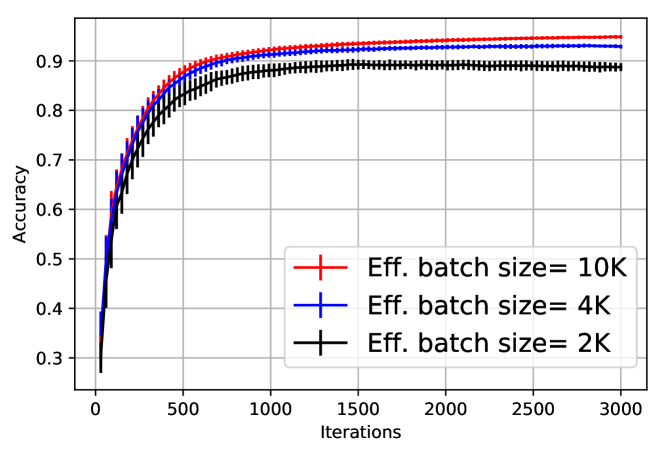
(a) MNIST

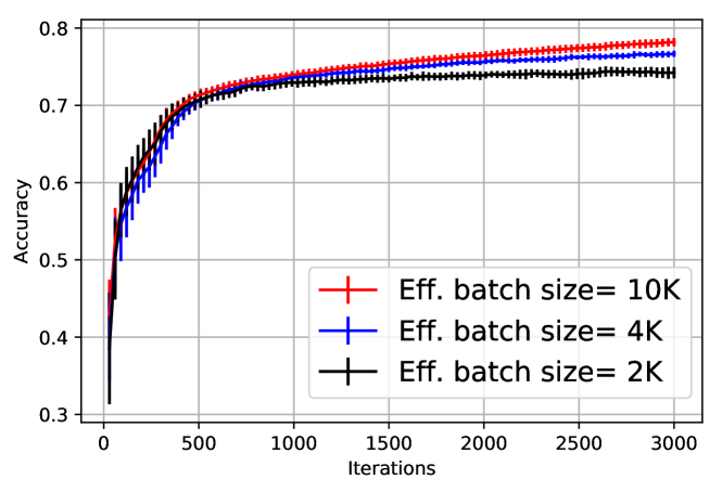
(b) Fashion-MNIST

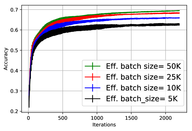
(c) CIFAR-10

Figure 2: Accuracy vs iterations tradeoff on various data sets, with local differential privacy-per-record-per-iteration $\varepsilon_{\ell e}=1.8$ for CIFAR-10, and $\varepsilon_{\ell e}=1.9$ for MNIST and Fashion-MNIST. The plots are over at least ten independent runs.

Note on central differential privacy: Since we are translating local differential privacy guarantees to central differential privacy guarantees, our notion of central differential privacy is in the replacement model, i.e., two neighboring data sets of the same size but differ by one record. However, the results in [42, 44, 43] are in the add/removal model, i.e., two neighboring data sets differ in the presence or absence of one data record. As a blackbox, for any algorithm, $\varepsilon_{\mathrm{Add/Remove}}\leq\varepsilon_{\mathrm{Replace}}\leq 2\varepsilon_{\mathrm{Add/Remove}}$, and for commonly used algorithms, the upper bound is close to tight.

Open question: We believe that the current accounting for central differential privacy via advanced composition is potentially loose, and one may get stronger guarantees via Rényi differential privacy accounting (similar to that in [42]). We leave the problem of tightening the overall central differential privacy guarantee for future work.

Estimating lower bounds through membership inference attacks: We use the membership inference attack to measure the privacy leakage of a model [45, 46, 47, 48]. While these measurements yield loose lower bounds on how much information is leaked by a model, it can serve as an effective comparison across models trained with noise subject to different privacy analyses (with their separate upper bounds on differential privacy).

Along the lines of Yeom et al. [46], for each model, we measure the average log-loss between true labels and predicted outputs over a set of samples used in training and not in training. One measure of privacy leakage involves the best binary (threshold) classifier based on these loss values to distinguish between in-training and out-training examples. The resulting ROC curve of the classifier across different thresholds can be used to estimate a lower bound on the privacy parameter. Specifically, it is easy to strengthen the results in Yeom et al. [46] to show that the difference between the true positive rate (TPR) and false positive rate (FPR) at any threshold is bound by $1-e^{-\varepsilon}$ for a model satisfying $\varepsilon$-differential privacy. Thus, the lower bound $\varepsilon\geq-\log\left(\text{max}(\text{TPR}-\text{FPR})\right)$. The results are shown in Table XI for all models trained. As can be seen from the results, even though the $\varepsilon_{c}$ upper bound are different for models trained under the ESA framework and those with DPSGD, there is no much difference in the lower bound.

VIII Conclusions

This paper’s overall conclusion that it is feasible to implement high-accuracy statistical reporting with strong central privacy guarantees, as long as respondent’s randomized reports are anonymized by a trustworthy intermediary. Sufficient for this are a small set of primitives—applied within a relatively simple, abstract attack model—for both analysis techniques and practical technical mechanisms. Apart from anonymization itself, the most critical of these primitives are those that involve fragmenting of respondents’ randomized reports; first explored in the original ESA paper [2], such fragmentation turns out to be critical to achieving strong central privacy guarantees with high utility, in our empirical applications on real-world datasets. As we show here, those primitives are sufficient to achieve high utility for difficult tasks such as iterative training of deep-learning neural networks, while providing both central and local guarantees of differential privacy.

In addition, this paper makes it clear that when it comes to practical applications of anonymous, differentially-private reporting, significantly more exploration and empirical evaluation is needed, along with more refined analysis. Specifically, this need is made very clear by the discrepancy this paper finds between the utility and central privacy guarantees of anonymous one-hot-encoded LDP reports and anonymous sketch-based LDP reports, witch sketching parameters drawn from those used in real-world deployments. At the very least, this discrepancy highlights how practitioners must carefully choose the mechanisms they use in sketch-based encodings, and the parameters by which they tune those mechanisms, in order to achieve good tradeoffs for the dataset and task at hand. However, the lack of precise central privacy guarantees for anonymous sketch-based LDP reports also shows the pressing needs for better sketch constructions and analyses that properly account for the anonymity and fragmentation of respondents’ reports. While some recent work has started to look at better analysis of sketching (e.g., asymptotically [19]), practitioners should look towards the excellent tradeoffs shown here for one-hot-encoded LDP reports, until further, more practical results are derived in the large alphabet setting.

-A Missing details from Section III

Proof of Theorem III.1.

To prove removal LDP we use the reference distribution $\mathcal{R}_{0}$ to be randomized response with $\varepsilon_{\ell}$ on the $k$-dimensional all-zeros vector $\boldsymbol{0}$. For any $\boldsymbol{x}\in\mathcal{D}$ (represented as one-hot binary vector in $k$ dimensions), $\boldsymbol{x}$ and $\boldsymbol{0}$ differ in one position and therefore, by standard properties of randomized response Algorithm $\mathsf{att}\textsf{-}\mathsf{frag}(\mathcal{R}_{k\text{-RAPPOR}})$ computing $\hat{x}^{(j)}:=\mathcal{R}_{j}(x^{(j)},\varepsilon_{\ell})$ for $j\in[k]$ satisfies removal $\varepsilon_{\ell}$-local differential privacy. Furthermore, each $\hat{x}^{(j)}$ by itself is computed with (replacement) $\varepsilon_{\ell}$-DP. We obtain the central differential privacy guarantee (through amplification via shuffling) by invoking Lemma 1 with $\lambda=\frac{2n}{1+e^{\varepsilon_{\ell}}}$.

The lower bound of $14\log(4/\delta)$ for $\lambda$ translates (with some simplification) to an upper bound of $\varepsilon_{\ell}\leq\log n-\log(14\log(4/\delta))$ assumed in the Theorem statement. Furthermore, as $\lambda\geq 14\log(2/\delta)\geq 8\log(2/\delta)$, we have that $\lambda-\sqrt{2\lambda\log(2/\delta)}$ in Lemma 1 is at least $\lambda/2$. Simplifying the expression in (1), the central privacy guarantee for each individual bit of any $\hat{\boldsymbol{x}}$ is:

$$\varepsilon_{c}^{\sf bit} \leq\sqrt{\frac{64\log(4/\delta)}{\lambda}}=\sqrt{\frac{64(1+e^{\varepsilon_{\ell}})\log(4/\delta)}{2n}}$$

$$\leq\sqrt{\frac{64\cdot e^{\varepsilon_{\ell}}\log(4/\delta)}{n}}.$$ (2)

To prove removal central differential privacy for the entire output we define the algorithm $\mathcal{M}^{\prime}\colon\mathcal{D}^{n}\times 2^{[n]}$ as follows. Given $D=(x_{1},\ldots,x_{n})$ and a set of indices $I$, $\mathcal{M}^{\prime}$ uses the reference distribution $\mathcal{R}_{0}$ in place of the local randomizer for each element $x_{i}$ for which $i\not\in I$. Changing any $\boldsymbol{x}$ to $\boldsymbol{0}$ for the $i$-th element changes only one input bit. It follows from Eq. (2) that the overall $\varepsilon_{c}$ for removal central differential privacy guarantee is $\varepsilon_{c}=\sqrt{\frac{64\cdot e^{\varepsilon_{\ell}}\log(4/\delta)}{n}}$, which completes the proof. ∎

Proof of Theorem III.2.

In $\mathsf{att}\textsf{-}\mathsf{frag}(\mathcal{R}_{k\text{-RAPPOR}})$ (Algorithm 1) consider any $\boldsymbol{x}$ and the corresponding $\hat{\boldsymbol{x}}$, the list of randomized responses $\mathcal{R}_{j}(x^{(j)},\varepsilon_{\ell})$. For brevity, consider the random variable $\boldsymbol{\zeta}=\left(\frac{e^{\varepsilon_{\ell}}+1}{e^{\varepsilon_{\ell}}-1}\cdot\hat{}\boldsymbol{x}-\frac{1}{e^{\varepsilon_{\ell}}-1}\right)$. It follows that $\mathbb{E}\left[\boldsymbol{\zeta}\right]=\boldsymbol{x}$ and furthermore ${\sf Var}[\boldsymbol{\zeta}]=\frac{e^{\varepsilon_{\ell}}+1}{e^{\varepsilon_{\ell}}-1}-1=\Theta\left(1/e^{\varepsilon_{\ell}}\right)$. Using standard sub-Gaussian tail bounds, and taking an union bound over the domain $[k]$, one can show that w.p. at least $1-\beta$, over all $n$ respondents with data $\boldsymbol{x}_{i}$,

$$\alpha=\left\|\hat{\boldsymbol{h}}-\frac{1}{n}\sum\boldsymbol{x}_{i}\right\|_{\infty}=\Theta\left(\sqrt{\frac{\log(k/\beta)}{ne^{\varepsilon_{\ell}}}}\right).$$

Applying Theorem III.1 to compute $\varepsilon_{c}$ in terms of $\varepsilon_{\ell}$ completes the proof. ∎

-B Missing details from Section IV

We start by analyzing the privacy of an arbitrary combination of local DP randomizer followed by an arbitrary differentially private algorithm. To simplify this analysis we show that it suffices to restrict our attention to binary domains.

Lemma .1.

Assume that for every replacement $(\varepsilon_{1},\delta_{1})$-DP local randomizer $\mathcal{Q}_{1}\colon\{0,1\}\to\{0,1\}$ and every replacement $(\varepsilon_{2},\delta_{2})$-DP local randomizer $\mathcal{Q}_{2}\colon\{0,1\}\to\{0,1\}$ we have that $\mathcal{Q}_{2}\circ\mathcal{Q}_{1}$ is a replacement $(\varepsilon,\delta)$-DP local randomizer. Then for every replacement $(\varepsilon_{1},\delta_{1})$-DP local randomizer $\mathcal{R}_{1}\colon X\to Y$ and replacement $(\varepsilon_{2},\delta_{2})$-DP local randomizer $\mathcal{R}_{2}:Y\to Z$ we have that $\mathcal{R}_{2}\circ\mathcal{R}_{1}$ is a replacement $(\varepsilon,\delta)$-DP local randomizer.

Proof.

Let $\mathcal{R}_{1}\colon X\to Y$ be a replacement $(\varepsilon_{1},\delta_{1})$-local randomizer and $\mathcal{R}_{2}\colon Y\to Z$ be a replacement $(\varepsilon_{2},\delta_{2})$-DP randomizer. Assume for the sake of contradiction that for some $(\varepsilon,\delta)$ there exists an event $S\subseteq Z$ such that for some $x,x^{\prime}$:

$$\mathop{\mathbf{Pr}}[\mathcal{R}_{2}(\mathcal{R}_{1}(x))\in S]>e^{\varepsilon}\mathop{\mathbf{Pr}}[\mathcal{R}_{2}(\mathcal{R}_{1}(x^{\prime}))\in S]+\delta.$$

We will show that then there exist an $(\varepsilon_{1},\delta_{1})$-DP local randomizer $\mathcal{Q}_{1}\colon\{0,1\}\to\{0,1\}$ and $(\varepsilon_{2},\delta_{2})$-DP local randomizer $\mathcal{Q}_{2}\colon\{0,1\}\to\{0,1\}$ such that

$$\mathop{\mathbf{Pr}}[\mathcal{Q}_{2}(\mathcal{Q}_{1}(0))=1]>e^{\varepsilon}\mathop{\mathbf{Pr}}[\mathcal{Q}_{2}(\mathcal{Q}_{1}(1))=1]+\delta,$$

contradicting the conditions of the lemma.

Let

$$y_{0}:=\operatorname*{arg\,min}_{y\in Y}\{\mathop{\mathbf{Pr}}[\mathcal{R}_{2}(y)\in S]\},$$

$$y_{1}:=\operatorname*{arg\,max}_{y\in Y}\{\mathop{\mathbf{Pr}}[\mathcal{R}_{2}(y)\in S]\}$$

and let

$$P_{1}:=\{y\in Y\ |\ \mathop{\mathbf{Pr}}[\mathcal{R}_{1}(x)=y]-e^{\varepsilon}\mathop{\mathbf{Pr}}[\mathcal{R}_{1}(x^{\prime})=y]>0\}.$$

Using this definition and our assumption we get:

$$\left(\mathop{\mathbf{Pr}}[\mathcal{R}_{1}(x)\not\in P_{1}]-e^{\varepsilon}\mathop{\mathbf{Pr}}[\mathcal{R}_{1}(x^{\prime})\not\in P_{1}]\right)\cdot\mathop{\mathbf{Pr}}[\mathcal{R}_{2}(y_{0})\in S]$$

$$+\left(\mathop{\mathbf{Pr}}[\mathcal{R}_{1}(x)\in P_{1}]-e^{\varepsilon}\mathop{\mathbf{Pr}}[\mathcal{R}_{1}(x^{\prime})\in P_{1}]\right)\cdot\mathop{\mathbf{Pr}}[\mathcal{R}_{2}(y_{1})\in S]$$

$$\geq\sum_{y\in Y}\left(\mathop{\mathbf{Pr}}[\mathcal{R}_{1}(x)=y]-e^{\varepsilon}\mathop{\mathbf{Pr}}[\mathcal{R}_{1}(x^{\prime})=y]\right)\cdot\mathop{\mathbf{Pr}}[\mathcal{R}_{2}(y)\in S]$$

$$>\delta.$$

We now define $\mathcal{Q}_{1}(0):=\mathbbm{1}\left(\mathcal{R}_{1}(x)\in P_{1}\right)$ and $\mathcal{Q}_{1}(1):=\mathbbm{1}\left(\mathcal{R}_{1}(x^{\prime})\in P_{1}\right)$, where $\mathbbm{1}\left(\cdot\right)$ denotes the indicator function. By this definition $\mathcal{Q}_{1}$ is obtained from $\mathcal{R}_{1}$ by restricting the set of inputs and postprocessing the output. Thus $\mathcal{Q}_{1}$ is a replacement $(\varepsilon_{1},\delta_{1})$-DP local randomizer. Next define for $b\in\{0,1\}$, $\mathcal{Q}_{2}(b):=\mathbbm{1}\left(\mathcal{R}_{2}(y_{b})\in S\right)$. Again, it is easy to see that $\mathcal{Q}_{2}$ is a replacement $(\varepsilon_{2},\delta_{2})$-DP. We now obtain that

$$\mathop{\mathbf{Pr}}[\mathcal{Q}_{2}(\mathcal{Q}_{1}(0))=1]-e^{\varepsilon}\mathop{\mathbf{Pr}}[\mathcal{Q}_{2}(\mathcal{Q}_{1}(1))=1]$$

$$=\sum_{b\in\{0,1\}}\left(\mathop{\mathbf{Pr}}[\mathcal{Q}_{1}(0)=b]-e^{\varepsilon}\mathop{\mathbf{Pr}}[\mathcal{Q}_{1}(1)=b]\right)\cdot\mathop{\mathbf{Pr}}[\mathcal{Q}_{2}(b)=1]$$

$$=\left(\mathop{\mathbf{Pr}}[\mathcal{R}_{1}(x)\not\in P_{1}]-e^{\varepsilon}\mathop{\mathbf{Pr}}[\mathcal{R}_{1}(x^{\prime})\not\in P_{1}]\right)\cdot\mathop{\mathbf{Pr}}[\mathcal{R}_{2}(y_{0})\in S]$$

$$+\left(\mathop{\mathbf{Pr}}[\mathcal{R}_{1}(x)\in P_{1}]-e^{\varepsilon}\mathop{\mathbf{Pr}}[\mathcal{R}_{1}(x^{\prime})\in P_{1}]\right)\cdot\mathop{\mathbf{Pr}}[\mathcal{R}_{2}(y_{1})\in S]$$

$$>\delta$$

as needed for contradiction. ∎

As an easy corollary of Lemma .1 we obtain a tight upper bound in the pure differential privacy case.

Corollary .2.

For every replacement $\varepsilon_{1}$-DP local randomizer $\mathcal{R}_{1}\colon X\to Y$ and every replacement $\varepsilon_{2}$-DP local randomizer $\mathcal{R}_{2}\colon Y\to Z$ we have that $\mathcal{R}_{2}\circ\mathcal{R}_{1}$ is a replacement $\varepsilon$-DP local randomizer for $\varepsilon=\ln\left(\frac{e^{\varepsilon_{1}+\varepsilon_{2}}+1}{e^{\varepsilon_{1}}+e^{\varepsilon_{2}}}\right)$. In addition, if $\mathcal{R}_{1}$ is removal $\varepsilon_{1}$-DP then $\mathcal{R}_{2}\circ\mathcal{R}_{1}$ is a removal $\varepsilon$-DP.

Proof.

By Lemma .1 it suffices to consider the case where $X=Y=Z=\{0,1\}$. Thus it suffices to upper bound the expression:

$$\frac{\mathop{\mathbf{Pr}}[\mathcal{R}_{1}(0)=0]\cdot\mathop{\mathbf{Pr}}[\mathcal{R}_{2}(0)=1]+\mathop{\mathbf{Pr}}[\mathcal{R}_{1}(0)=1]\cdot\mathop{\mathbf{Pr}}[\mathcal{R}_{2}(1)=1]}{\mathop{\mathbf{Pr}}[\mathcal{R}_{1}(1)=0]\cdot\mathop{\mathbf{Pr}}[\mathcal{R}_{2}(0)=1]+\mathop{\mathbf{Pr}}[\mathcal{R}_{1}(1)=1]\cdot\mathop{\mathbf{Pr}}[\mathcal{R}_{2}(1)=1]}.$$

Denoting by $p_{0}:=\mathop{\mathbf{Pr}}[\mathcal{R}_{1}(0)=0]$, $p_{1}:=\mathop{\mathbf{Pr}}[\mathcal{R}_{1}(1)=0]$ and $\alpha=\mathop{\mathbf{Pr}}[\mathcal{R}_{2}(0)=1]/\mathop{\mathbf{Pr}}[\mathcal{R}_{2}(1)=1]$ the expression becomes:

$$\frac{1+(\alpha-1)p_{0}}{1+(\alpha-1)p_{1}}.$$

The conditions on $\mathcal{R}_{1}$ imply that $\frac{p_{0}}{p_{1}},\frac{1-p_{0}}{1-p_{1}}\in[e^{-\varepsilon_{1}},e^{\varepsilon_{1}}]$ and $\alpha\in[e^{-\varepsilon_{2}},e^{\varepsilon_{2}}]$. Without loss of generality we can assume that $\alpha\geq 1$ and thus the expression is maximized when $\alpha=e^{\varepsilon_{2}}$ and $p_{0}>p_{1}$. Maximizing the expression under these constraints we obtain that the maximum is $\frac{e^{\varepsilon_{1}+\varepsilon_{2}}+1}{e^{\varepsilon_{1}}+e^{\varepsilon_{2}}}$ and is achieved when $p_{0}=1-p_{1}=e^{\varepsilon_{1}}/(1+e^{\varepsilon_{1}})$. In particular, the claimed value of $\varepsilon$ is achieved by the standard binary randomized response with $\varepsilon_{1}$ and $\varepsilon_{2}$.

To deal with the case of removal we can simply substitute $\mathcal{R}_{1}(x^{\prime})$ with the reference distribution $\mathcal{R}_{0}$ in the analysis to obtain removal DP guarantees for $\mathcal{R}_{2}\circ\mathcal{R}_{1}$. ∎

We remark that it is easy to see that $\frac{e^{\varepsilon_{1}+\varepsilon_{2}}+1}{e^{\varepsilon_{1}}+e^{\varepsilon_{2}}}\leq\min\{e^{\varepsilon_{1}},e^{\varepsilon_{2}}\}$. Also in the regime where $\varepsilon_{1},\varepsilon_{2}\leq 1$ we obtain that $\varepsilon=O(\varepsilon_{1}\varepsilon_{2})$, namely the privacy is amplified by applying local randomization.

Proof of Theorem IV.2.

The proof of local differential privacy is immediate based on Theorem IV.1. To obtain the central differential privacy guarantee, we consider each of the terms in the $\min$ expression for $\varepsilon_{c}$. From the central differential privacy context, each of the shufflers in the execution of Algorithm 2 can be considered to be a post-processing of the output of a single shuffler, and the privacy guarantee from this single shuffler should prevail. Each of the individual reports are at most $\varepsilon_{b}$-locally differentially private, and hence by using the generic privacy amplification by shuffling result from Lemma II.5, the second term in the $\varepsilon_{c}$ follows. To obtain the first term, recall the matrix $M(\boldsymbol{x})$ in Section IV. Each row of the matrix satisfies $\varepsilon_{0}$-local differential privacy, and there are $\tau$ rows in this matrix. Hence, first applying privacy amplification theorem from Lemma 1 on each of the rows independently, and then using advanced composition from Theorem II.7 over the $\tau$ rows, we obtain the first term in $\varepsilon_{c}$, which completes the proof of the central differential privacy guarantee.

The utility guarantee follows immediately from the utility proof of Theorem III.2. ∎

-C Missing Details from Section V

Proof of Theorem V.1.

The proof follows a similar argument as [49, Theorem 3.5]. Consider two neighboring data sets $D$ and $D^{\prime}$, there are only two crowd IDs whose counts get affected. Since the randomization for each of the counts are done independently, we can analyze their privacy independently and then perform standard composition [34]. Consider a crowd $\mathcal{D}_{i}$, and the corresponding counts $n_{i}\neq n^{\prime}_{i}$ on data sets $D$ and $D^{\prime}$ respectively.

Notice that the computation of $\hat{n}_{i}$ satisfies $\frac{\varepsilon_{\ell}^{\sf cr}}{2}$-differential privacy by the Laplace mechanism [23]. Now, by the tail probability of Laplace noise, with probability at least $1-\frac{\delta^{\sf cr}}{2}$, the algorithm does not abort on crowd $\mathcal{D}_{i}$. In that case, the shuffler can ensure $\hat{n}_{i}$ records in $\mathcal{D}_{i}$ via dropping records. This would ensure $\left(\frac{\varepsilon_{\ell}^{\sf cr}}{2},\frac{\delta^{\sf cr}}{2}\right)$-differential privacy.

Therefore, composing the above over the two crowds that are affected by $D$ and $D^{\prime}$, we complete the proof. ∎

Proof of Theorem V.2.

The proof of this theorem follows from standard tail probabilities of the Laplace mechanism. With probability at least $1-\delta^{\sf cr}$, for a given crowd $\mathcal{D}_{i}$, the error in the reported count is at most $2T=\frac{4}{\varepsilon_{\ell}^{\sf cr}}\log\left(\frac{4}{\delta^{\sf cr}}\right)$. Taking an union bound over all the $\xi$ crowds, completes the proof. ∎

-D Missing Details from Section VI

Proof of Theorem VI.1.

We will prove the privacy and utility guarantees separately.

Privacy guarantee: We will prove this guarantee in two steps: (i) Amplify the local differential privacy guarantee $\varepsilon_{\ell}$ per epoch via [29, Corollary 5.3.1] (see Theorem .3), and (ii) Use advanced composition [49] to account for the privacy budget. Combination of these two immediately implies the theorem.

Theorem .3 (Corollary 5.1 from [29]).

Let $\mathcal{R}:\mathbb{X}\to\mathbb{Y}$ be an $\varepsilon_{\ell e}$-local differentially private randomizer, and $\mathcal{M}$ be the corresponding shuffled mechanism (that shuffles all the locally randomized reports). If $\varepsilon_{\ell e}\leq\log(n)/4$, then $\mathcal{M}$ satisfies $\left(O\left(\frac{(e^{\varepsilon_{\ell e}}-1)\sqrt{\log(1/\delta)}}{\sqrt{n}}\right),\delta\right)$-central differential privacy in the shuffled setting.

Utility guarantee: Here we use the a standard bound on the convergence of Stochastic Gradient Descent (SGD) stated in Theorem .4. One can instantiate Theorem .4 in the context of this paper as follows: $F(\theta)=\frac{1}{n}\sum\limits_{i=1}^{n}\ell(\theta;x_{i})$, and $\boldsymbol{g}_{t}$ is the randomized gradient computed in Algorithm 5.

Theorem .4 (Theorem 2 from [50]).

Consider a convex function $F:\mathcal{C}\to\mathbb{R}$ defined over a convex set $\mathcal{C}\subseteq\mathbb{R}^{d}$, and consider the following SGD algorithm: $\theta_{t+1}\leftarrow\Pi_{\mathcal{C}}\left(\theta_{t}-\frac{c}{\sqrt{t}}\boldsymbol{g}_{t}\right)$, where $\Pi_{\mathcal{C}}\left(\cdot\right)$ is the $\ell_{2}$-projection operator onto the set $\mathcal{C}$, $c>0$ is a constant, and $\boldsymbol{g}_{t}$ has the following properties. i) [Unbiasedness] $\mathop{\mathbf{E}}[\boldsymbol{g}_{t}]=\bigtriangledown F(\theta_{t})$, and ii) [Bounded Variance] $\mathop{\mathbf{E}}\left[\|\boldsymbol{g}_{t}\|^{2}_{2}\right]=G^{2}$. The following is true for any $T>1$.

$$\mathop{\mathbf{E}}[F(\theta_{t})]-\min\limits_{\theta\in\mathcal{C}}F(\theta)\leq\left(\frac{\|\mathcal{C}\|^{2}_{2}}{c}+cG^{2}\right)\frac{2+\log T}{\sqrt{T}}.$$

Following the instantiation above, by the property of the noise distribution, one can easily show that $\mathop{\mathbf{E}}[\boldsymbol{g}_{t}]=\frac{1}{n}\sum\limits_{i=1}^{n}\bigtriangledown\ell(\theta_{t};x_{i})$, and furthermore $\mathop{\mathbf{E}}[\|\boldsymbol{g}_{t}\|_{2}]=O\left(\frac{L\sqrt{d}}{\sqrt{n}}\cdot\frac{e^{\varepsilon_{\ell e}}+1}{e^{\varepsilon_{\ell e}}-1}\right)=G$. (See [17, Appendix I.2] for the full derivation. Setting $c=\frac{\|\mathcal{C}\|_{2}}{G}$, and setting $T=n/\log^{2}n$ completes the proof. ∎

References

- [1] Ú. Erlingsson, V. Pihur, and A. Korolova, “RAPPOR: Randomized aggregatable privacy-preserving ordinal response,” in Proc. of the 2014 ACM Conf. on Computer and Communications Security (CCS’14). ACM, 2014, pp. 1054–1067.
- [2] A. Bittau, Ú. Erlingsson, P. Maniatis, I. Mironov, A. Raghunathan, D. Lie, M. Rudominer, U. Kode, J. Tinnes, and B. Seefeld, “Prochlo: Strong privacy for analytics in the crowd,” in Proc. of the 26th ACM Symp. on Operating Systems Principles (SOSP’17), 2017.
- [3] Ú. Erlingsson, V. Feldman, I. Mironov, A. Raghunathan, K. Talwar, and A. Thakurta, “Amplification by shuffling: From local to central differential privacy via anonymity,” in Proceedings of the Thirtieth Annual ACM-SIAM Symposium on Discrete Algorithms. SIAM, 2019, pp. 2468–2479.
- [4] A. Cheu, A. Smith, J. Ullman, D. Zeber, and M. Zhilyaev, “Distributed differential privacy via mixnets,” CoRR, vol. abs/1808.01394, 2018. [Online]. Available: http://arxiv.org/abs/1808.01394
- [5] J. Valentino-DeVries, “Uncovering what your phone knows,” The New York Times, Dec. 2018, https://www.nytimes.com/2018/12/14/reader-center/phone-data-location-investigation.html.
- [6] S. L. Warner, “Randomized response: A survey technique for eliminating evasive answer bias,” J. of the American Statistical Association, vol. 60, no. 309, pp. 63–69, 1965.
- [7] Apple’s differential privacy team, “Learning with privacy at scale,” https://machinelearning.apple.com/docs/learning-with-privacy-at-scale/appledifferentialprivacysystem.pdf, 2018.
- [8] R. Dingledine, N. Mathewson, and P. Syverson, “Tor: The second-generation onion router,” in 13th USENIX Security Symp., 2004, pp. 21–21.
- [9] D. Lazar, Y. Gilad, and N. Zeldovich, “Karaoke: Distributed private messaging immune to passive traffic analysis,” in 13th USENIX Symp. on Operating Systems Design and Implementation (OSDI’18), 2018, pp. 711–725.
- [10] H. Corrigan-Gibbs and D. Boneh, “Prio: Private, robust, and scalable computation of aggregate statistics,” in Proc. of the 14th USENIX Conf. on Networked Systems Design and Implementation (NSDI), 2017, pp. 259–282.
- [11] K. Bonawitz, V. Ivanov, B. Kreuter, A. Marcedone, H. B. McMahan, S. Patel, D. Ramage, A. Segal, and K. Seth, “Practical secure aggregation for privacy-preserving machine learning,” in Proc. of the 2017 ACM Conf. on Computer and Communications Security (CCS), 2017, pp. 1175–1191.
- [12] E. Roth, D. Noble, B. Hemenway Falk, and A. Haeberlen, “Honeycrisp: Large-scale differentially private aggregation without a trusted core,” in Proceedings of the 27th ACM Symposium on Operating Systems Principles (SOSP’19), Oct. 2019.
- [13] A. Cheu, A. Smith, J. Ullman, D. Zeber, and M. Zhilyaev, “Distributed differential privacy via shuffling,” in Annual International Conference on the Theory and Applications of Cryptographic Techniques. Springer, 2019, pp. 375–403.
- [14] B. Balle, G. Barthe, and M. Gaboardi, “Privacy amplification by subsampling: Tight analyses via couplings and divergences,” CoRR, vol. abs/1807.01647, 2018. [Online]. Available: http://arxiv.org/abs/1807.01647
- [15] R. Bassily and A. Smith, “Local, private, efficient protocols for succinct histograms,” in Proc. of the Forty-Seventh Annual ACM Symp. on Theory of Computing (STOC’15), 2015, pp. 127–135.
- [16] R. Bassily, K. Nissim, U. Stemmer, and A. Thakurta, “Practical locally private heavy hitters,” in Advances in Neural Information Processing Systems (NIPS), 2017, pp. 2288–2296.
- [17] J. C. Duchi, M. I. Jordan, and M. J. Wainwright, “Minimax optimal procedures for locally private estimation,” Journal of the American Statistical Association, vol. 113, no. 521, pp. 182–201, 2018.
- [18] G. Fanti, V. Pihur, and Ú. Erlingsson, “Building a RAPPOR with the unknown: Privacy-preserving learning of associations and data dictionaries,” Proc. on Privacy Enhancing Technologies (PoPETS), vol. 2016, no. 3, pp. 41–61, 2016.
- [19] B. Ghazi, N. Golowich, R. Kumar, R. Pagh, and A. Velingker, “Private heavy hitters and range queries in the shuffled model,” arXiv preprint arXiv:1908.11358, 2019.
- [20] J. Tang, A. Korolova, X. Bai, X. Wang, and X. Wang, “Privacy loss in Apple’s implementation of differential privacy on macOS 10.12,” CoRR, vol. abs/1709.02753, 2017. [Online]. Available: http://arxiv.org/abs/1709.02753
- [21] A. Kwon, H. Corrigan-Gibbs, S. Devadas, and B. Ford, “Atom: Horizontally scaling strong anonymity,” in Proceedings of the 26th Symposium on Operating Systems Principles, ser. SOSP ’17, 2017.
- [22] M. Lécuyer, R. Spahn, K. Vodrahalli, R. Geambasu, and D. Hsu, “Privacy accounting and quality control in the sage differentially private ml platform,” 2019.
- [23] C. Dwork, F. McSherry, K. Nissim, and A. Smith, “Calibrating noise to sensitivity in private data analysis,” in Proc. of the Third Conf. on Theory of Cryptography (TCC), 2006, pp. 265–284. [Online]. Available: http://dx.doi.org/10.1007/11681878_14
- [24] C. Dwork, “Differential privacy,” in Proc. of the 33rd International Conf. on Automata, Languages and Programming—Volume Part II (ICALP), 2006, pp. 1–12.
- [25] C. Dwork, K. Kenthapadi, F. McSherry, I. Mironov, and M. Naor, “Our data, ourselves: Privacy via distributed noise generation,” in Advances in Cryptology—EUROCRYPT, 2006, pp. 486–503.
- [26] G. Cormode and S. Muthukrishnan, “An improved data stream summary: the count-min sketch and its applications,” Journal of Algorithms, vol. 55, no. 1, pp. 58–75, 2005.
- [27] M. Bun, J. Nelson, and U. Stemmer, “Heavy hitters and the structure of local privacy,” in Proceedings of the 37th ACM SIGMOD-SIGACT-SIGAI Symposium on Principles of Database Systems. ACM, 2018, pp. 435–447.
- [28] A. Smith, A. Thakurta, and J. Upadhyay, “Is interaction necessary for distributed private learning?” in 2017 IEEE Symposium on Security and Privacy (SP). IEEE, 2017, pp. 58–77.
- [29] B. Balle, J. Bell, A. Gascon, and K. Nissim, “The privacy blanket of the shuffle model,” in Advances in Cryptology—CRYPTO, 2019.
- [30] Y. Ishai, E. Kushilevitz, R. Ostrovsky, and A. Sahai, “Cryptography from anonymity,” in 2006 47th Annual IEEE Symposium on Foundations of Computer Science (FOCS’06). IEEE, 2006, pp. 239–248.
- [31] B. Balle, J. Bell, A. Gascon, and K. Nissim, “Differentially private summation with multi-message shuffling,” arXiv preprint arXiv:1906.09116, 2019.
- [32] C. Dwork, G. N. Rothblum, and S. Vadhan, “Boosting and differential privacy,” in Proc. of the 51st Annual IEEE Symp. on Foundations of Computer Science (FOCS), 2010, pp. 51–60.
- [33] M. Bun and T. Steinke, “Concentrated differential privacy: Simplifications, extensions, and lower bounds,” in Theory of Cryptography Conference. Springer, 2016, pp. 635–658.
- [34] C. Dwork and A. Roth, “The algorithmic foundations of differential privacy,” Foundations and Trends in Theoretical Computer Science, vol. 9, no. 3–4, pp. 211–407, 2014.
- [35] P. Kairouz, S. Oh, and P. Viswanath, “Extremal mechanisms for local differential privacy,” Journal of Machine Learning Research, vol. 17, no. 17, pp. 1–51, 2016. [Online]. Available: http://jmlr.org/papers/v17/15-135.html
- [36] H. B. McMahan, D. Ramage, K. Talwar, and L. Zhang, “Learning differentially private language models without losing accuracy,” CoRR, vol. abs/1710.06963, 2017. [Online]. Available: http://arxiv.org/abs/1710.06963
- [37] R. Bassily, V. Feldman, K. Talwar, and A. Guha Thakurta, “Private stochastic convex optimization with optimal rates,” in Advances in Neural Information Processing Systems 32, 2019, pp. 11 279–11 288.
- [38] O. Williams and F. McSherry, “Probabilistic inference and differential privacy,” in Advances in Neural Information Processing Systems, 2010, pp. 2451–2459.
- [39] S. Song, K. Chaudhuri, and A. D. Sarwate, “Stochastic gradient descent with differentially private updates,” in 2013 IEEE Global Conference on Signal and Information Processing. IEEE, 2013, pp. 245–248.
- [40] R. Bassily, A. Smith, and A. Thakurta, “Private empirical risk minimization: Efficient algorithms and tight error bounds,” in Proc. of the 2014 IEEE 55th Annual Symp. on Foundations of Computer Science (FOCS), 2014, pp. 464–473.
- [41] C. Ledig, L. Theis, F. Huszár, J. Caballero, A. Cunningham, A. Acosta, A. Aitken, A. Tejani, J. Totz, Z. Wang et al., “Photo-realistic single image super-resolution using a generative adversarial network,” in Proceedings of the IEEE conference on computer vision and pattern recognition, 2017, pp. 4681–4690.
- [42] M. Abadi, A. Chu, I. J. Goodfellow, H. B. McMahan, I. Mironov, K. Talwar, and L. Zhang, “Deep learning with differential privacy,” in Proc. of the 2016 ACM SIGSAC Conf. on Computer and Communications Security (CCS’16), 2016, pp. 308–318.
- [43] Anonymous, “Making the shoe fit: Architectures, initializations, and tuning for learning with privacy,” https://openreview.net/forum?id=rJg851rYwH.
- [44] Google, “Tensorflow-privacy,” https://github.com/tensorflow/privacy.
- [45] R. Shokri, M. Stronati, C. Song, and V. Shmatikov, “Membership inference attacks against machine learning models,” in 2017 IEEE Symposium on Security and Privacy (SP), 2017, pp. 3–18.
- [46] S. Yeom, I. Giacomelli, M. Fredrikson, and S. Jha, “Privacy risk in machine learning: Analyzing the connection to overfitting,” in 2018 IEEE 31st Computer Security Foundations Symposium (CSF), Jul. 2018, pp. 268–282.
- [47] B. Jayaraman and D. Evans, “Evaluating differentially private machine learning in practice,” in USENIX Security Symposium, 2019, pp. 1895–1912.
- [48] Úlfar Erlingsson, I. Mironov, A. Raghunathan, and S. Song, “That which we call private,” 2019.
- [49] S. Vadhan, “The complexity of differential privacy,” in Tutorials on the Foundations of Cryptography. Springer, 2017, pp. 347–450.
- [50] O. Shamir and T. Zhang, “Stochastic gradient descent for non-smooth optimization: Convergence results and optimal averaging schemes,” in International Conference on Machine Learning, 2013, pp. 71–79.