Learning credit assignment

Abstract

Deep learning has achieved impressive prediction accuracies in a variety of scientific and industrial domains. However, the nested non-linear feature of deep learning makes the learning highly non-transparent, i.e., it is still unknown how the learning coordinates a huge number of parameters to achieve a decision making. To explain this hierarchical credit assignment, we propose a mean-field learning model by assuming that an ensemble of sub-networks, rather than a single network, are trained for a classification task. Surprisingly, our model reveals that apart from some deterministic synaptic weights connecting two neurons at neighboring layers, there exist a large number of connections that can be absent, and other connections can allow for a broad distribution of their weight values. Therefore, synaptic connections can be classified into three categories: very important ones, unimportant ones, and those of variability that may partially encode nuisance factors. Therefore, our model learns the credit assignment leading to the decision, and predicts an ensemble of sub-networks that can accomplish the same task, thereby providing insights toward understanding the macroscopic behavior of deep learning through the lens of distinct roles of synaptic weights.

Introduction.— As deep neural networks become an increasingly important tool in diverse domains of scientific and engineering applications Krizhevsky et al. (2012); Hannun et al. (2014); He et al. (2015); Silver et al. (2017); Richards et al. (2019), the black box properties of the tool turn out to be a challenging obstacle puzzling researchers in the field Sinz et al. (2019). In other words, the decision making behavior of a network output can not be easily understood in terms of interactions among building components of the network. This shares the same spirit as another long-standing puzzle in theory of the brain—how the emergent behavior of a neuronal population hierarchy can be traced back to its elements Sinz et al. (2019); Richards et al. (2019). This challenging issue is the well-known credit assignment problem (CAP), determining how much credit a given component (either neuron or connection) should take for a particular behavior output Richards et al. (2019). To solve this problem, one needs to bridge the gap between microscopic interactions of components and macroscopic behavior.

Excitingly, recent works showed that there exist sub-networks of random weights that are able to produce better-than-chance accuracies Frankle and Carbin (2018); Zhou et al. (2019); Ramanujan et al. (2019). This property seems to be universal across different architectures, datasets and computational tasks Morcos et al. (2019). Even one can start with no connections and add complexity as needed by assuming a single shared weight parameter Gaier and Ha (2019). Moreover, it was recently revealed that the innate template of face-selective neurons can spontaneously emerge from sufficient statistical variations present in the random initial wirings of neural circuits, while the template may be fine-tuned during early visual experiences Baek et al. (2019). Therefore, from both artificial and biological neural networks perspectives, exploring how and why these random wirings exist will definitely provide us a powerful lens through which we can better understand and even further improve the computational capacities of deep neural networks.

Here, we propose a statistical model of learning credit assignment from training data of a computational task. According to the model, we search for an optimal random network ensemble as an inductive bias about the hypothesis space Sinz et al. (2019). The hypothesis space is composed of all candidate networks with different assignments of weight values that accomplish the computation task. Consistent with previous studies Frankle and Carbin (2018); Zhou et al. (2019); Ramanujan et al. (2019), the optimal ensemble contains sub-networks of the original full network, which further allows for capturing uncertainty in the hypothesis space. The model can be solved by mean-field methods, thereby providing a physics interpretation of how credit assignment occurs in a hierarchical deep neural system.

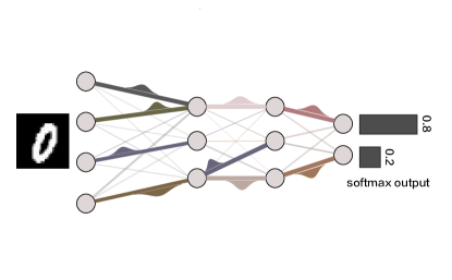
Figure 1: The schematic illustration of the model learning credit assignment. A deep neural network of four layers including two hidden layers is used to recognize a handwritten digit, say zero, with the softmax output indicating the probability of the categorization. Each connection is specified by a spike and slab distribution, where the spike indicates the probability of the absence of this connection, and the slab is modeled by a Gaussian distribution of weight values as pictorially shown only on strong connections with different means and variances. Other weak connections indicate nearly unit spike probabilities, although they also carry a slab distribution (not shown in the illustration for simplicity).

Model.— To learn credit assignment, we search for an optimal random neural network ensemble to accomplish a classification task of handwritten digits mni . More precisely, we design a deep neural network of $L$ layers, including $L-2$ hidden layers. The depth of the network $L$ can be made arbitrarily large. The size (width) of the $l$-th layer is denoted by $N_{l}$, therefore $N_{1}$ is determined by the total number of pixels in an input image, and $N_{L}$ is the number of classes (e.g., $10$ for the handwritten digit dataset). The weight value of the connection from neuron $i$ at the upstream layer $l$ to neuron $k$ at the downstream layer $l+1$ is defined by $w_{ik}^{l}$, and the activation of the neuron $k$ at the $(l+1)$-th layer $h_{k}^{l+1}$ is a non-linear function of the pre-activation $z_{k}^{l+1}=\frac{1}{\sqrt{N_{l}}}\sum_{i}w_{ik}^{l}h_{i}^{l}$, where the weight scaling factor $1/\sqrt{N_{l}}$ ensures that the weighted sum is independent of the upstream layer width. We use the rectified linear unit (ReLU) function Nair and Hinton (2010) as the transfer function from pre-activation $z$ to activation $h$ defined as $h={\rm max}(0,z)$. The output transfer function specifies a probability over all classes of the input image by using a softmax function $h_{k}=\frac{e^{z_{k}}}{\sum_{i}e^{z_{i}}}$ where $z_{i}$ is the pre-activation of the $i$-th neuron at the output layer. For the categorization task, we define $\hat{h}_{i}$ as the target label (one-hot representation), and use the cross entropy $\mathcal{C}=-\sum_{i}\hat{h}_{i}\ln h_{i}$ as the objective function to be minimized.

Training the neural network corresponds to adjusting all connection weights to minimize the cross entropy until the network is able to classify unseen handwritten digits with a satisfied accuracy (so-called generalization ability). Therefore, after the network is trained with a training data size of $T$, the network’s generalization ability is verified with a test data size of $V$. Remarkably, the state-of-the-art test accuracy is able to surpass the human performance in some complex tasks He et al. (2015). However, the decision making behavior of the output neurons in a deep network is still challenging to understand in terms of computational principles of single building components (either neurons or weights). Recent empirical machine learning works showed that a subnetwork of random weights can produce a better-than-chance accuracy Frankle and Carbin (2018); Ramanujan et al. (2019); Zhou et al. (2019). This clearly suggests that there may exist a random ensemble of neural networks that fulfill the computational task given the width and depth of the deep network. This ensemble may occupy a tiny portion of the entire model space. Therefore, a naive random initialization of the neural network can only yield a chance-level accuracy. To incorporate all these challenging issues into a theoretical model, we propose to model the weight by a spike and slab (SaS) distribution as follows:

$$P(w_{ik}^{l})=\pi_{ik}^{l}\delta(w_{ik}^{l})+(1-\pi_{ik})\mathcal{N}(w_{ik}^{l}|m_{ik}^{l},\Xi_{ik}^{l}),$$ (1)

where the discrete probability mass at zero defines the spike, and the slab is characterized by a Gaussian distribution with mean $m_{ik}^{l}$ and variance $\Xi_{ik}^{l}$ over a continuous domain (see Fig. 1 for an illustration).

The SaS distribution has been widely used in statistics literatures Mitchell and Beauchamp (1988); Ishwaran and Rao (2005). Here, the spike and slab have respectively their own physics interpretations in learning credit assignment of neural networks. The spike is intimately related to the concept of network compression Han et al. (2015); Ullrich et al. (2017); Morcos et al. (2019), where not all resources of connections are used in a task. This parameter allows to identify very important weights, and further evaluate remaining capacities for learning new tasks Parisi et al. (2019). A recent physics study has already showed that a deep neural network can be robust against connection removals Huang and Goudarzi (2018). The slab continuous support characterizes the ensemble of neural networks with random weights producing better-than-chance accuracies. Among these weights, some are very important, indicated by a vanishing spike probability mass, and could thus explain the decision making of the output neurons, while the variance of the corresponding Gaussian distribution captures the uncertainty of the decision making solutions McClure and Kriegeskorte (2016). Therefore, the inductive bias of connections and their associated weights can be learned through the SaS model of credit assignment. Note that the Gaussian slab is not used here as an additional regularization complexity term in the objective function Nowlan and Hinton (1992). Instead, the continuous slab is combined coherently with the spike probability to model the uncertainty of weights facing noisy sensory inputs (Fig. 1).

Next, we derive a mean-field method to learn the SaS parameters $\bm{\theta}_{ik}^{l}\equiv(\pi_{ik}^{l},m_{ik}^{l},\Xi_{ik}^{l})$ for all layers. The first and second moments of the weight $w_{ik}^{l}$ are given by $\mu_{ik}^{l}\equiv\mathbb{E}[w_{ik}^{l}]=m_{ik}^{l}(1-\pi_{ik}^{l})$ and $\varrho_{ik}^{l}\equiv\mathbb{E}[(w_{ik}^{l})^{2}]=(1-\pi_{ik}^{l})[\Xi_{ik}^{l}+(m_{ik}^{l})^{2}]$, respectively. Given a large width of the layer, the central-limit-theorem implies that the pre-activation follows approximately a Gaussian distribution $\mathcal{N}(z_{i}^{l}|G_{i}^{l},(\Delta_{i}^{l})^{2})$, where the mean and variance are given respectively by

$$G_{i}^{l} =\frac{1}{\sqrt{N_{l-1}}}\sum_{k}\mu_{ki}^{l-1}h_{k}^{l-1},$$ (2a)

$$(\Delta_{i}^{l})^{2} =\frac{1}{N_{l-1}}\sum_{k}(\varrho_{ki}^{l-1}-(\mu_{ki}^{l-1})^{2})(h_{k}^{l-1})^{2}.$$ (2b)

Then, the feedforward transformation of the input signal can be re-parametrized by Shayer et al. (2017); Huang (2020)

$$z_{i}^{l} =G_{i}^{l}+\epsilon_{i}^{l}\Delta_{i}^{l},$$ (3a)

$$h_{i}^{l} ={\rm ReLU}(z_{i}^{l}),$$ (3b)

for $l<L$. The last layer uses the softmax function. $\epsilon_{i}^{l}$ is a layer- and component-dependent standard Gaussian random variable with zero mean and unit variance. $\bm{\epsilon}^{l}$ is quenched for every single training mini-epoch and the same value is used in both forward and backward computations. This reparametrization retains the statistical structure in Eq. (2). The objective function relies on $(\bm{\mu},\bm{\varrho})$ that can be preserved by a transformation of $\bm{\theta}$. Hence, we use a regularization strength to control the $\ell_{2}$-norm of $\bm{m}$ and $\bm{\Xi}$. In addition, the transformation does not change the fraction of $\pi=1$ or $0$ SM , maintaining the qualitative behavior of the model.

Learning of the hyper-parameter $\bm{\theta}_{ik}^{l}$ can be achieved by a gradient descent of the objective function, i.e.,

$$\Delta\bm{\theta}_{ki}^{l}=-\eta\mathcal{K}_{i}^{l+1}\frac{\partial z_{i}^{l+1}}{\partial\bm{\theta}_{ki}^{l}}$$ (4)

where $\eta$ denotes the learning rate, and $\mathcal{K}_{i}^{l+1}\equiv\frac{\partial\mathcal{C}}{\partial z_{i}^{l+1}}$. The entire dataset is divided into minibatches over which the gradients are evaluated. Note that unlike the standard back-propagation (BP) Rumelhart David E. et al. (1986), we adapt the SaS distribution rather than a particular weight, in accord with our motivation of learning statistical features of the hypothesis space for a particular computation task (e.g., image classification here).

On the top layer, $\mathcal{K}_{i}^{L}$ can be directly estimated as $\mathcal{K}_{i}^{L}=-\hat{h}_{i}^{L}(1-h_{i}^{L})$ by definition. For lower layers, $\mathcal{K}_{i}^{l}$ can be estimated by using the chain rule, resulting in a back-propagation equation of the error signal from the top layer:

$$\mathcal{K}_{i}^{l} =\delta_{i}^{l}f^{\prime}(z_{i}^{l}),$$ (5a)

$$\delta_{i}^{l} =\sum_{k}\mathcal{K}_{k}^{l+1}\frac{\partial z_{k}^{l+1}}{\partial h_{i}^{l}},$$ (5b)

where $\delta_{i}^{l}\equiv\frac{\partial\mathcal{C}}{\partial h_{i}^{l}}$, and $f^{\prime}(\cdotp)$ denotes the derivative of the transfer function.

To proceed, we have to compute $\frac{\partial z_{k}^{l+1}}{\partial h_{i}^{l}}$ and $\frac{\partial z_{i}^{l+1}}{\partial\bm{\theta}_{ki}^{l}}$. The first derivative characterizes how sensitive the pre-activation is under the change of the input activity of one neuron, and this response is computed as follows:

$$\frac{\partial z_{k}^{l+1}}{\partial h_{i}^{l}}=\frac{\mu_{ik}^{l}}{\sqrt{N_{l}}}+\frac{(\varrho_{ik}^{l}-(\mu_{ik}^{l})^{2})h_{i}^{l}}{N_{l}\Delta_{k}^{l+1}}\epsilon_{k}^{l+1}.$$ (6)

The second derivative characterizes how sensitive the pre-activation is under the change of the hyper-parameters of the SaS distribution. Because the mean and variance, $G_{i}^{l+1}$ and $\Delta_{i}^{l+1}$, is a function of the hyper-parameters, the second derivative for each hyper-parameter can be derived similarly as follows:

$$\frac{\partial z_{i}^{l+1}}{\partial m_{ki}^{l}} =\frac{(1-\pi_{ki}^{l})h_{k}^{l}}{\sqrt{N_{l}}}+\frac{\mu_{ki}^{l}\pi_{ki}^{l}}{N_{l}\Delta_{i}^{l+1}}(h_{k}^{l})^{2}\epsilon_{i}^{l+1},$$ (7a)

$$\frac{\partial z_{i}^{l+1}}{\partial\pi_{ki}^{l}} =-\frac{m_{ki}^{l}h_{k}^{l}}{\sqrt{N_{l}}}-\frac{(2\pi_{ki}^{l}-1)(m_{ki}^{l})^{2}+\Xi_{ki}^{l}}{2N_{l}\Delta_{i}^{l+1}}(h_{k}^{l})^{2}\epsilon_{i}^{l+1},$$ (7b)

$$\frac{\partial z_{i}^{l+1}}{\partial\Xi_{ki}^{l}} =\frac{1-\pi_{ki}^{l}}{2N_{l}\Delta_{i}^{l+1}}(h_{k}^{l})^{2}\epsilon_{i}^{l+1}.$$ (7c)

Eq. (6) and Eq. (7) share the same form with the pre-activation $z_{i}^{l}$ [Eq. (3)], due to the reparametrization trick used to handle the uncertainty of weights in the hypothesis space. Therefore, the learning process of our model naturally captures the fluctuation of the hypothesis space, highlighting the significant difference from the standard BP which computes only a point estimate of the connection weights. In particular, if we enforce $\bm{\pi}=0$ and $\bm{\Xi}=0$, $\mathbf{m}$ becomes identical to the weight configuration, thus our learning equations will immediately recover the standard BP algorithm Rumelhart David E. et al. (1986). Therefore, our learning protocol can be thought of as a generalized back-propagation (gBP) at the weight distribution level, or the candidate-network ensemble level.

Our framework is a cheap way to compute the posterior distribution of the weights given the data, which can be alternatively realized by a Bayesian inference where a variational free energy is commonly optimized through Monte-Carlo samplings Blei et al. (2017); Huang (2020); Baldock and Marzari (2019). The optimization of the variational free energy for deep neural networks is computationally challenging, especially for the SaS prior whose entropy has no analytic form as well. In contrast, gBP stores two times more parameters than BP, while other computational steps are exactly the same; the training time is affordable, as a typical deep network training scales linearly with the number of parameters Sejnowski (2020).

We remark that during learning, the spike mass $\pi$ should be clipped as ${\rm max}(0,{\rm min}(1,\pi))$, and the variance $\Xi\leftarrow{\rm max}(0,\Xi)$. Learning the SaS model allows for credit assignment to each connection, considering a network ensemble realizing the same task. An effective network can be constructed by sampling the learned SaS distribution.

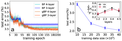
Figure 2: Properties of gBP in testing performances on unseen data. (a) Training trajectories of a network architecture of three or four layers. The architecture is defined as 784-100-100-10 (four layers) or 784-100-10 (three layers), where each number indicates the corresponding layer width. Networks are trained on the data size of $T=10^{4}$ images and tested on another unseen-data size of $V=10^{4}$ images. The fluctuation is computed from five independent runs. (b) Test errors of gBP versus training data size. The error bar characterizes the fluctuation across ten independently-sampled network architectures from the SaS distribution. The same network of four layers as in (a) is used. The inset shows the sparsity per connection as a function of layers, for which networks of five layers are used and the hidden layer width is still $100$ nodes. Each marker is an average over ten independent runs. k in the inset means the training data size in the unit of $10^{3}$.

The size of the hypothesis space can be approximated by the model entropy $S=-\int_{\mathbb{R}^{\mathcal{D}}}P(\bm{w})\ln P(\bm{w})d\bm{w}$, where $\mathcal{D}$ is the number of weight parameters in the network. Because the joint distribution of weights is assumed to be factorized across individual connections, $S=\sum_{\ell}S_{\ell}$, where the entropy contribution of each individual connection ($\ell$) is expressed as SM

$$S_{\ell}=-\pi_{\ell}\ln\Biggl{[}\pi_{\ell}+(1-\pi_{\ell})\mathcal{N}(0|m_{\ell},\Xi_{\ell})\Biggr{]}-\frac{(1-\pi_{\ell})}{\mathcal{B}}\sum_{s}\Gamma(\epsilon_{s}),$$ (8)

where $\mathcal{B}$ denotes the number of standard Gaussian random variables $\epsilon_{s}$, and $\Gamma(\epsilon_{s})=\ln\Bigl{[}\pi_{\ell}\delta(m_{\ell}+\sqrt{\Xi_{\ell}}\epsilon_{s})+\frac{(1-\pi_{\ell})}{\sqrt{\Xi_{\ell}}}\mathcal{N}(\epsilon_{s}|0,1)\Bigr{]}$. If $\pi_{\ell}=0$, the entropy $S_{\ell}$ can be analytically computed as $\frac{1}{2}\ln(2\pi e\Xi_{\ell})$. If $\Xi_{\ell}=0$, the Gaussian distribution reduces to a Dirac delta function, and the entropy becomes an entropy of discrete random variables.

Results.— Despite working at the synaptic weight distribution level, gBP can reach a similar even better test accuracy than that of BP [Fig. 2 (a)]. As expected, the test error for gBP decreases with training data size [Fig. 2 (b)]. The error bar implies that effective networks sampled from the learned SaS distribution still yield accurate predictions, confirming the network ensemble assumption. Our theory also reveals that the sparsity, obtained from the statistics of $\{\pi_{ij}^{l}\}$, grows first and then decreases [the inset of Fig. 2 (b)], suggesting that the actual working network does not used up all synaptic connections, consistent with empirical observations of network compression Han et al. (2015); Mallya and Lazebnik (2018); Morcos et al. (2019) and theoretical studies of toy models Huang and Goudarzi (2018); Li and Saad (2020). Along hierarchical stages of the deep neural network, the initial stage is responsible for encoding, therefore the sparsity must be low to ensure that there is sufficient space for encoding the important information, while at the middle stage, the encoded information is re-coded through hidden representations, suggesting that the noisy information is further distilled, which may explain why the sparsity goes up. Finally, to guarantee the feature-selective information being extracted, the sparsity must drop to yield an accurate classification. Therefore, our model can interpret the deep learning as an encoding-recoding-decoding process, as also argued in a biological neural hierarchy Pitkow and Angelaki (2017).

To inspect more carefully what distribution of hyper-parameters gBP learned, we plot Fig. 3 (a) showing the evolution of the distribution across the hierarchical stages. First, the spike mass $\bm{\pi}$ has a U-shaped distribution. One extreme is at $\pi=0$, suggesting that the corresponding connection carries feature-selective information and thus can not be pruned, while the other extreme is at $\pi=1$, suggesting that the corresponding connection can be completely pruned. Apart from these two extremes, there exist a relatively small number of connections which can be present or absent with certain probabilities. These connections may reflect nuisance factors in sensory inputs Achille and Soatto (2018). The mean of the slab distribution has a relatively broad distribution, but the peak is located around zero; an L-shaped distribution of the variance hyper-parameter is observed. Note that if $\Xi=0$, the SaS distribution reduces to a Bernoulli distribution with two delta peaks. Due to Eq. (7b), the point solution $(\bm{\pi}=0,\bm{\Xi}=0)$ is not a stable attractor for gBP SM . Moreover, as the training data size increases, the variance per connection displays a non-monotonic behavior with a residual value depending on the hierarchical stage SM .

We can use the entropy $S_{\ell}$ for each connection to characterize the variability of the weight value. Note that the entropy can be negative for continuous random variables. The peak at zero [Fig. 3 (b)] indicates that a large number of connections are deterministic, including two cases: (i) $\pi=1$ (unimportant (UIP) weight); (ii) $\pi=0$ and $\Xi=0$ (very important (VIP) weight). Fig. 3 (c) shows that the entropy per connection grows first, and then decreases. This non-monotonic behavior is the same with that of the sparsity in Fig. 2 (b). The large entropy at the middle stage suggests that during the recoding process, the network has more degrees of freedom to manipulate the hypothesis space of the computational task Zou and Huang (2020). Furthermore, more training data reduce the uncertainty (yet not to zero) until saturation [Fig. 3 (c)].

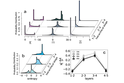
Figure 3: Statistical properties of trained four-layer networks with gBP. Unless stated otherwise, other training conditions are the same as in Fig. 2. (a) Distribution of hyper-parameters $(\bm{\pi},\mathbf{m},\bm{\Xi})$ for a typical trained network. (b) Distribution of connection entropy $S_{\ell}$ for a typical trained network. (c) Entropy per connection versus layers ($\mathcal{B}=100$). Different training data sizes are considered, and the result is averaged over ten independent runs of five-layer networks.

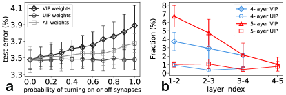
Figure 4: Effects of targeted-weight perturbation on test performances. Training conditions are the same as in Fig. 2, and the result is averaged over ten independent runs. (a) VIP weights and all weights (without weight categorization) are stochastically turned off, keeping the same number, while UIP weights are stochastically turned on and sampled from a standard Gaussian distribution. The perturbation is carried out at the first hierarchical stage of a four-layer network. (b) The fraction of VIP and UIP weights between neighboring layers.

Finally, our mean-field framework can be used to explore effects of targeted-weight perturbation [Fig. 4 (a)], which previous studies of random deep models could not address Huang and Goudarzi (2018); Li and Saad (2020). VIP weights play a significant role in determining the generalization capability, while turning on UIP weights does not impair the performance. A random dilution of all weights behaves mildly in between. When going deeper, the perturbation effect becomes less evident (not shown), due to the less number of VIP weights [Fig. 4 (b)].

Conclusion.— In this work, we propose a statistical model of learning credit assignment in deep neural networks, resulting in an optimal random sub-network ensemble explaining the behavior output of the hierarchical system. The model can be solved by using mean-field methods, yielding a practical way to visualize consumed resources of connections and an ensemble of random weights—two key factors affecting the emergent decision making behavior of the network. Our framework can be applied to a more challenging CIFAR-$10$ dataset Krizhevsky (2009) and obtains qualitatively similar results SM . Our model thus provides deep insights towards understanding many recent interesting empirical observations of random templates in both artificial and biological neural networks Frankle and Carbin (2018); Ramanujan et al. (2019); Zhou et al. (2019); Baek et al. (2019); Zador (2019). The model also provides a principled method for network compression saving memory and computation demands Han et al. (2015), and could also have implications for continual learning of sequential tasks, where those important connections for old tasks are always protected to learn new tasks Kirkpatrick et al. (2017); Mallya and Lazebnik (2018).

As artificial neural networks become increasingly important to model the brain Richards et al. (2019); Baek et al. (2019), our current study of artificial neural networks may provide cues for addressing how the brain solves the credit assignment problem. Other promising directions include considering correlations among weights and generalization of this framework to the temporal credit assignment, where spatio-temporal information is considered in training recurrent neural networks Werbos (1990); Sussillo and Abbott (2009); Marblestone et al. (2016).