Obtaining higher-order Galerkin accuracy
when the boundary is polygonally approximated
Abstract.
We study two techniques for correcting the geometrical error associated with domain approximation by a polygon. The first was introduced some time ago [2] and leads to a nonsymmetric formulation for Poisson’s equation. We introduce a new technique that yields a symmetric formulation and has similar performance. We compare both methods on a simple test problem.
1. Introduction
When a Dirichlet problem on a smooth domain is approximated by a polygon, an error occurs that is suboptimal for quadratic approximation [1, 10, 11]. However, this can be corrected by a modification of the variational form [2]. Here we review this approach and suggest a new one.
Let be a smooth, bounded, two-dimensional domain. Consider the Poisson equation with Dirichlet boundary conditions:
| (1) |
We assume that and are sufficiently smooth that can be extended to be in , where contains a neighborhood of the closure of .
One way to discretize (1) is to approximate the domain by polygons , where the edge lengths of are of order in size. Then conventional finite elements can be employed, with the Dirichlet boundary conditions being approximated by the assumption that on [3], with appropriately defined. For example, let us suppose for the moment that and we take as well. In particular, we assume that is triangulated with a quasi-uniform mesh of maximum triangle size , and the boundary vertices of are in . We define where
Then the standard finite element approximation finds satisfying
| (2) |
where . Here we assume that is extended smoothly outside of .
This approach for (piecewise linear approximation) leads to the error estimate
However, when this approach is applied with piecewise quadratic polynomials (), the best possible error estimate is
| (3) |
which is less than optimal order by a factor of . The reason of course is that we have made only a piecewise linear approximation of . Table 1 summarizes some computational experiments for the test problem in Section 2.1. We see a significant improvement for quadratics over linears, but there is almost no improvement with cubics. Moreover, we will see that a significant improvement using quadratics can be obtained using simple approaches that modify the variational form.
There have been many techniques introduced to circumvent the loss of accuracy with quadratics (and higher-order piecewise polynomials) [11, 6]. However, all of them require some modification of the quadrature for the elements at the boundary.
Here we review an approach by Bramble et al. [2] that solves directly on , but with a modified variational form based on the method of Nitsche [6]. The method [2] has been modified and applied in many ways [4]. However, the method in [2] leads to a non symmetric bilinear form. Given this shortcoming we define a new method that is symmetric and solves the problem on that has similar convergence results. As we will see in the next section, one main idea in [2] is that one uses a Taylor series of the solution near the boundary to define appropriate boundary conditions on . We should mention that this idea has been used recently (see for example [5, 8]).
| L2 err | rate | H1 err | rate | seg | hmax | ||
|---|---|---|---|---|---|---|---|
| 1 | 2 | 1.84e+00 | NA | 6.25e+00 | NA | 10 | 1.05e+00 |
| 1 | 4 | 2.93e-01 | 2.65 | 1.89e+00 | 1.73 | 20 | 4.94e-01 |
| 1 | 8 | 9.55e-02 | 1.62 | 1.06e+00 | 0.83 | 40 | 2.61e-01 |
| 1 | 16 | 2.47e-02 | 1.95 | 5.45e-01 | 0.96 | 80 | 1.35e-01 |
| 2 | 2 | 4.18e-01 | NA | 1.41e+00 | NA | 10 | 1.05e+00 |
| 2 | 4 | 9.44e-02 | 2.15 | 4.26e-01 | 1.73 | 20 | 4.94e-01 |
| 2 | 8 | 2.30e-02 | 2.04 | 1.59e-01 | 1.42 | 40 | 2.61e-01 |
| 2 | 16 | 5.62e-03 | 2.03 | 5.45e-02 | 1.54 | 80 | 1.35e-01 |
| 3 | 2 | 3.17e-01 | NA | 8.25e-01 | NA | 10 | 1.05e+00 |
| 3 | 4 | 8.81e-02 | 1.85 | 2.94e-01 | 1.49 | 20 | 4.94e-01 |
| 3 | 8 | 2.22e-02 | 1.99 | 1.07e-01 | 1.46 | 40 | 2.61e-01 |
| 3 | 16 | 5.53e-03 | 2.01 | 3.82e-02 | 1.49 | 80 | 1.35e-01 |
2. The Bramble-Dupont-Thomée approach
(a) (b)
(b) 
The method [2] of Bramble-Dupont-Thomée (BDT) achieves high-order accuracy by modifying Nitsche’s method [6] applied on . We assume that and we do not necessarily assume that the boundary vertices of belong to . The bilinear form used in [2] is
| (4) |
Here, denotes the outward-directed normal to and
Contrast the definition of to the closely related function defined by
For simplicity the assume that . Then the BDT method will find such that
If were 0, this would be Nitsche’s method on .
Corrections of arbitrary order, involving terms for are studied in [2], but for simplicity we restrict attention to the first-order correction to Nitsche’s method given in (4). The error estimates obtained in [2] are as follows
where
Thus using the variational form (4) leads to an approximation that is optimal-order with quadratics and cubics and is only suboptimal for quartics by a factor of .
(a)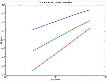 (b)
(b)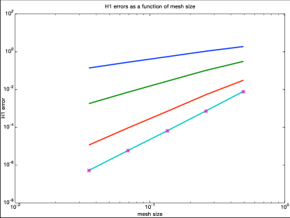
2.1. An example of a circle
We consider a numerical example. Consider the case where is a disc of radius centered at the origin, in which case we have . However, it is more difficult to evaluate . We have for , where denotes the outward normal to . We can write , and . Since , we have
Then
Note that for , and . Since , we must pick the plus sign, so
It is not hard to see that in this case.
This problem is simple to implement using the FEniCS Project code dolfin [7]. We take , , and in the computational experiments described subsequently. Computational results for this example are given in Table 2 where we see optimal order approximation for , improvement for over (suboptimal by a factor ), and no improvement for quintics. These errors are depicted in Figure 2.
| hmax | L2 error | rate | H1 error | rate | ||
|---|---|---|---|---|---|---|
| 1 | 8 | 0.261 | 0.0947 | 1.61 | 1.06 | 0.82 |
| 1 | 16 | 0.135 | 0.0245 | 1.95 | 0.544 | 0.96 |
| 1 | 32 | 0.0688 | 0.00639 | 1.94 | 0.277 | 0.97 |
| 1 | 64 | 0.0353 | 0.00158 | 2.02 | 0.137 | 1.02 |
| 2 | 8 | 0.261 | 2.81e-03 | 2.61 | 0.103 | 1.57 |
| 2 | 16 | 0.135 | 3.70e-04 | 2.93 | 0.0277 | 1.89 |
| 2 | 32 | 0.0688 | 4.77e-05 | 2.96 | 0.00717 | 1.95 |
| 2 | 64 | 0.0353 | 5.91e-06 | 3.01 | 0.00179 | 2.00 |
| 3 | 8 | 0.261 | 1.56e-04 | 3.92 | 5.31e-03 | 2.54 |
| 3 | 16 | 0.135 | 9.44e-06 | 4.05 | 7.06e-04 | 2.91 |
| 3 | 32 | 0.0688 | 5.81e-07 | 4.02 | 9.23e-05 | 2.94 |
| 3 | 64 | 0.0353 | 3.57e-08 | 4.02 | 1.15e-05 | 3.00 |
| 4 | 8 | 0.261 | 1.49e-04 | 3.96 | 7.41e-04 | 3.42 |
| 4 | 16 | 0.135 | 9.29e-06 | 4.00 | 6.63e-05 | 3.48 |
| 4 | 32 | 0.0688 | 5.80e-07 | 4.00 | 5.90e-06 | 3.49 |
| 4 | 64 | 0.0353 | 3.63e-08 | 4.00 | 5.22e-07 | 3.50 |
| 5 | 8 | 0.261 | 1.47e-04 | 3.96 | 7.10e-04 | 3.41 |
| 5 | 16 | 0.135 | 9.27e-06 | 3.99 | 6.44e-05 | 3.46 |
| 5 | 32 | 0.0688 | 5.80e-07 | 4.00 | 5.77e-06 | 3.48 |
| 5 | 64 | 0.0353 | 3.62e-08 | 4.00 | 5.12e-07 | 3.49 |
3. A new method based on a Robin-type approach
One issue with the BDT method is that the resulting linear system is not symmetric, although it is possible to symmetrize the method as we discuss in Section 8. Here we develop a technique that leads to a symmetric system. Moreover, this method does not require the parameter(s) from Nitsche’s method. For Nitsche’s method to succeed, must be chosen appropriately [9].
We first separate to its piecewise linear part and its curvilinear part. We will assume that where is a piecewise linear segment and are and no where linear. We let the end points of to be .
For the method in this section we assume that the vertices of belong to and hence might not be a subdomain of . Hence, we need to define in this case. We assume that for every that is there is a unique smallest number in absolute value such that
We assume that the approximate domain boundary can be decomposed into three parts, as follows. Let be the edges of .
| (5) |
where denotes the interior of . Let . We assume the following.
Assumption 1.
We assume that all the vertices of belong to and that each (for ) is a vertex of . Finally, we assume that
Our method is based on a Robin type of boundary condition on . In fact, our method will be based on the closely related problem:
Here we define for and not a vertex of . The key here is that, using that vanishes on , for ( not a vertex of ) we have
| (6) |
where lies in the line segment with end points and .
Now we can write the method. We start by defining the finite element space we will use
Also define
where is a suitable approximation of and is a piecewise polynomial of degree at most on .
The bilinear form is given by
where
Then the method solves:
Find such that
| (7) |
Here
where is the linear interpolant onto . Note that we can define only knowing on . Alternatively, if we have an analytic representation of we can define as a smooth extension of outside of .
4. Error Analysis
4.1. Stability Analysis
Unfortunately, the bilinear form is not positive definite. However, we will be able to prove stability of method. In order to do so, we need to decompose the space into its boundary contribution and interior contribution. More precisely, we can write
where . We will define a norm on :
and a semi-norm
Note that is in fact a norm on .
The following crucial lemma will allow us to prove stability.
Lemma 1.
There exists a constant such that
| (8) |
Proof.
Let be the collection of edges that are a subset of and let be triangles such that has an edge in . Then, if and using inverse estimates we have
The result is complete after we use that for . ∎
We note that may not be well defined for all . Therefore, we need to make an assumption on such that this is not the case.
Assumption 2.
We assume that is such that
| (9) |
For example, if has a lower bound as follows, then (9) will hold. Suppose that the end points of are and . Then we assume that there exists a constant and a such that
where is independent of . Under these conditions, Assumption 2 holds.
We can now prove the stability result.
Theorem 1.
Proof.
We know we can write where and . Define by
Note that . Now we can estimate .
Hence, we have
We can now prove error estimates after we make an assumption more stringent than Assumption 2.
Assumption 3.
Suppose that the end points of are and . Then we assume that there exists a constant such that
where is independent of .
Note that this assumption does not allow and to be tangent on the vertices of . Assumption 3 implies Assumption 2; in particular, the example after Assumption 2 holds with .
Theorem 2.
Proof.
We let . Then we see that
where , and .
Note that using integration by parts we have
First consider then we have
However, we have
Therefore, we get
∎
Hence,
Now lets consider . If we let then
Hence,
Now let we then have
Let , with end points and . Then, we have . Hence, using Assumption 3 we get
Thus,
We then obtain the following estimate, after summing over all edges ,
We get the following inequality after using approximation properties of the Lagrange interpolant:
Therefore, we have
Combining the above results we get
The result now follows from Theorem 1.
5. Implementation
One feature of Nitsche’s method, that is preserved with BDT, is that one uses the full space of piecewise polynomials without restriction at the boundary. The modification of to obtain the space of piecewise polynomials vanishing at boundary vertices is not trivial to implement in automated systems like FEniCS [7].
Thus it is of interest to consider a simplification to the Robin-type method (7) which removes this constraint. Thus we define, for ,
where . We then define and .
For implementation issues we solve by
| (11) |
The computational experiments used this approach. The answers do not depend on for small, as indicated in Table 3. We were even able to have for (11) using dolfin.
| segs | hmax | L2 err | H1 err | bdry err | |||
| 2 | 64 | 320 | 3.5e-02 | 1.0e-04 | 1.1e-03 | 2.1e-03 | 1.3e-01 |
| 2 | 64 | 320 | 3.5e-02 | 1.0e-05 | 1.1e-04 | 1.8e-03 | 2.5e-02 |
| 2 | 64 | 320 | 3.5e-02 | 1.0e-06 | 1.2e-05 | 1.8e-03 | 3.2e-03 |
| 2 | 64 | 320 | 3.5e-02 | 1.0e-07 | 6.0e-06 | 1.8e-03 | 3.2e-04 |
| 2 | 64 | 320 | 3.5e-02 | 1.0e-08 | 5.9e-06 | 1.8e-03 | 4.3e-05 |
| 2 | 64 | 320 | 3.5e-02 | 1.0e-09 | 5.9e-06 | 1.8e-03 | 3.1e-05 |
| 2 | 64 | 320 | 3.5e-02 | 1.0e-10 | 5.9e-06 | 1.8e-03 | 3.1e-05 |
| 2 | 128 | 640 | 1.8e-02 | 1.0e-07 | 1.3e-06 | 4.4e-04 | 6.4e-04 |
| 2 | 128 | 640 | 1.8e-02 | 1.0e-08 | 7.3e-07 | 4.4e-04 | 6.5e-05 |
| 2 | 128 | 640 | 1.8e-02 | 1.0e-09 | 7.2e-07 | 4.4e-04 | 7.3e-06 |
| 2 | 128 | 640 | 1.8e-02 | 1.0e-10 | 7.2e-07 | 4.4e-04 | 3.9e-06 |
| 2 | 128 | 640 | 1.8e-02 | 1.0e-11 | 7.2e-07 | 4.4e-04 | 3.9e-06 |
| 2 | 256 | 1280 | 9.0e-03 | 1.0e-09 | 8.9e-08 | 1.1e-04 | 1.3e-05 |
| 2 | 256 | 1280 | 9.0e-03 | 1.0e-10 | 8.9e-08 | 1.1e-04 | 1.3e-06 |
| 2 | 256 | 1280 | 9.0e-03 | 1.0e-11 | 8.9e-08 | 1.1e-04 | 4.9e-07 |
| 2 | 256 | 1280 | 9.0e-03 | 1.0e-12 | 8.9e-08 | 1.1e-04 | 4.9e-07 |
6. Computational Experiments
6.1. Example of a circle
We return now to the computational test problem described in Section 2.1. It is not difficult to show that Assumption 3 holds for the meshes we used. We see from Table 4 that the error is optimal order for , consistent with Theorem 2. In these cases, the error is also optimal order, and the boundary error is higher order for quadratics. For our numerical experiments seem to predict the error
which coincides with Theorem 2.
(a)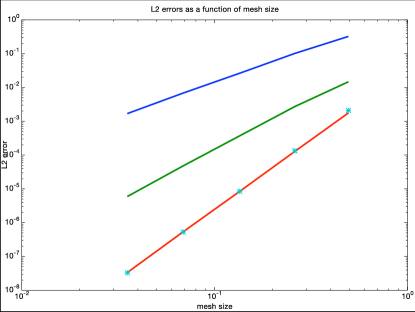 (b)
(b)
| hmax | L2 error | rate | H1 error | rate | bdry err | rate | ||
|---|---|---|---|---|---|---|---|---|
| 1 | 16 | 0.135 | 0.0264 | 1.95 | 0.545 | 0.96 | 0.292 | 1.04 |
| 1 | 32 | 0.0688 | 0.00683 | 1.95 | 0.277 | 0.98 | 0.145 | 1.01 |
| 1 | 64 | 0.0353 | 0.00169 | 2.01 | 0.137 | 1.02 | 0.0724 | 1.00 |
| 2 | 16 | 0.135 | 3.71e-04 | 2.88 | 0.0278 | 1.90 | 0.00177 | 2.71 |
| 2 | 32 | 0.0688 | 4.80e-05 | 2.95 | 0.00719 | 1.95 | 2.52e-04 | 2.81 |
| 2 | 64 | 0.0353 | 5.94e-06 | 3.02 | 0.00179 | 2.00 | 3.12e-05 | 3.02 |
| 3 | 16 | 0.135 | 8.43e-06 | 3.94 | 7.07e-04 | 2.91 | 5.22e-04 | 2.98 |
| 3 | 32 | 0.0688 | 5.39e-07 | 3.97 | 9.25e-05 | 2.93 | 6.52e-05 | 3.00 |
| 3 | 64 | 0.0353 | 3.35e-08 | 4.00 | 1.15e-05 | 3.01 | 8.13e-06 | 3.01 |
| 4 | 16 | 0.135 | 8.43e-06 | 3.99 | 7.07e-05 | 3.45 | 5.34e-04 | 2.97 |
| 4 | 32 | 0.0688 | 5.27e-07 | 4.00 | 6.38e-06 | 3.47 | 6.74e-05 | 2.99 |
| 4 | 64 | 0.0353 | 3.29e-08 | 4.00 | 5.69e-07 | 3.49 | 8.47e-06 | 2.99 |
| 5 | 16 | 0.135 | 8.43e-06 | 3.99 | 6.80e-05 | 3.45 | 5.35e-04 | 2.97 |
| 5 | 32 | 0.0688 | 5.27e-07 | 4.00 | 6.11e-06 | 3.48 | 6.75e-05 | 2.99 |
| 5 | 64 | 0.0353 | 3.30e-08 | 4.00 | 5.45e-07 | 3.49 | 8.47e-06 | 2.99 |
6.2. An example with
Now consider the case where is a disc of radius centered at the origin, having a concentric disc of radius removed. Again, it is not difficult to show that Assumption 3 holds for our meshes.
For boundary value problem, we take and , with
in the computational experiments described in Table 5. Note that vanishes on both boundary arcs. Note that the error estimates are consistent with Theorem 2.
| hmax | L2 error | H1 error | bdry error | ||
|---|---|---|---|---|---|
| 2 | 16 | 0.132 | 8.76e-04 | 6.87e-02 | 1.39e-04 |
| 2 | 32 | 0.070 | 1.20e-04 | 1.84e-02 | 9.64e-06 |
| 2 | 64 | 0.036 | 1.54e-05 | 4.68e-03 | 6.51e-07 |
| 3 | 16 | 0.132 | 2.90e-05 | 2.29e-03 | 6.59e-05 |
| 3 | 32 | 0.070 | 1.89e-06 | 3.07e-04 | 4.13e-06 |
| 3 | 64 | 0.036 | 1.17e-07 | 3.93e-05 | 2.47e-07 |
| 4 | 16 | 0.132 | 2.23e-05 | 3.37e-04 | 7.24e-05 |
| 4 | 32 | 0.070 | 1.39e-06 | 2.97e-05 | 4.57e-06 |
| 4 | 64 | 0.036 | 8.10e-08 | 2.61e-06 | 2.76e-07 |
7. Boundary layers
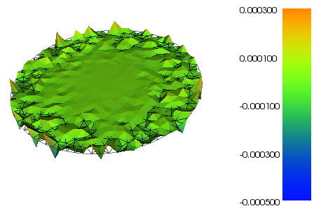
It is natural to expect the error with various boundary approximations might be limited to a boundary layer, with the interior error of a smaller magnitude. Our observations indicate something like this, but the behavior is more complex. In Figure 4, we see two computations done on the same mesh based on a triangulation of with having 80 segments and using piecewise-quadratic approximation. In Figure 4(a), we see the simple polygonal approximation (2). In this case, the error is somewhat larger near the boundary, but it does not decay to zero in the interior. Thus there is a significant pollution effect away from the boundary. On the other hand, Figure 4(b) shows what happens if the Robin-like method (7). Now we see that the error does decay towards zero in the interior, with the majority of the error concentrated at the boundary.
(a)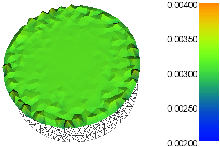 (b)
(b)
8. Higher order and symmetric methods
The Robin-type method presented in the previous section is at most of . High-order methods using the same techinique do not lead to symmetric systems. For simplicity assume that . Using that
we define
| (12) |
Unfortunately, is not symmetric.
One way to have higher-order, symmetric methods is by symmetrizing the approach of Bramble-Dupont-Thomée. Recall that Bramble et al. [2] developed arbitrary order methods, but that the bilinear forms are not symmetric. The lowest order method was presented in Section 2 where the bilinear is given by (4). One way to symmetrize and mainting the same convergence rates is by introducing the bilinear form:
This is precisely what is done in [4, (2.31)]. We see that
Note that is symmetric. We will investigate this and similar methods in the near future.
References
- [1] A. Berger, R. Scott, and G. Strang. Approximate boundary conditions in the finite element method. Symposia Mathematica, 10:295–313, 1972.
- [2] James H. Bramble, Todd Dupont, and Vidar Thomée. Projection methods for Dirichlet’s problem in approximating polygonal domains with boundary-value corrections. Mathematics of Computation, 26(120):869–879, 1972.
- [3] Susanne C. Brenner and L. Ridgway Scott. The Mathematical Theory of Finite Element Methods. Springer-Verlag, third edition, 2008.
- [4] Erik Burman, Peter Hansbo, and Mats G. Larson. A cut finite element method with boundary value correction. Mathematics of Computation, 2017.
- [5] Bernardo Cockburn and Manuel Solano. Solving Dirichlet boundary-value problems on curved domains by extensions from subdomains. SIAM J. Sci. Comput, 34 (1), no. 1: A497–A519, 2012.
- [6] Mika Juntunen and Rolf Stenberg. Nitsche’s method for general boundary conditions. Mathematics of Computation, 78(267):1353–1374, 2009.
- [7] A. Logg, K.A. Mardal, and G. Wells. Automated Solution of Differential Equations by the Finite Element Method: The FEniCS Book. Springer, 2012.
- [8] A. Main and G. Scovazzi. The shifted boundary method for embedded domain computations. Part I: Poisson and Stokes problems. J. Comput. Phys. 372, 972–995: 2018.
- [9] L. Ridgway Scott. Introduction to Automated Modeling with FEniCS. Computational Modeling Initiative, 2018.
- [10] R. Scott. Finite element techniques for curved boundaries. PhD thesis, Massachusetts Institute of Technology, 1973.
- [11] R. Scott. Interpolated boundary conditions in the finite element method. SIAM J. Numer. Anal., 12:404–427, 1975.