Design of QAM-FBMC Waveforms Considering MMSE Receiver

Abstract

Due to its high spectral confinement characteristics and spectral efficiency, QAM-FBMC is considered a candidate waveform to replace CP-OFDM. QAM-FBMC has inevitable non-orthogonality both in time and frequency, and the system and filter must be well-designed to minimize the interferences. However, existing QAM-FBMC studies utilize a matched filter as the receiver filter, which is not suitable for a non-orthogonal system. Therefore, in this paper, we design the prototype filters considering the MMSE criterion, and propose a system providing the highest SINR in QAM-FBMC which cannot avoid non-orthogonality. In addition, we confirm that the proposed filters show best performance at target SNR than the reference filters.

I Introduction

Filter-bank multi-carrier (FBMC) has been considered an alternative waveform to resolve the disadvantages of cyclic prefix-orthogonal frequency division multiplexing (CP-OFDM). The advantages of FBMC includes such as high out-band emission characteristics and the loss of spectral efficiency [1]. By subband filtering in the up-sampled frequency domain, the FBMC improves the spectral confinement characteristics dramatically, and can increase the spectral efficiency by reducing the guard band and the cyclic prefix. However, the conventional FBMC utilizes the offset-QAM (OQAM) for maintaining the orthogonality and this causes complicated signal processing on complex channels (such as multiple-input and multiple-output (MIMO) operation) due to the intrinsic interference problem [2, 3].

To avoid the problem of OQAM-FBMC, QAM-FBMC using non-orthogonal prototype filters has been proposed [4]. Instead of maintaining the orthogonality in the real domain through OQAM, QAM-FBMC uses QAM which increases the risk of giving up some degree of orthogonality in the complex domain. A QAM-FBMC filter designed to be non-orthogonal may degrade performance, but signal processing in the complex domain can easily be applied to QAM-FBMC in a way similar to CP-OFDM. The remaining major issue of QAM-FBMC is the need to design the system and filters to minimize the non-orthogonality that causes performance degradation.

There have been several previous studies on the problem of designing filters for QAM-FBMC. In the initial study, it was proposed to maximize the self-signal-to-interference ratio (self-SIR) by utilizing multiple base filters [4, 5]. In these studies, the QAM-FBMC system utilized different prototype filters for even and odd subcarriers, making the system complex. These filters were also poorly localized in the time domain, which presents a vulnerability problem for multipath channels in the FBMC system without CP. To overcome this problem, some studies have proposed design of a single prototype filter considering the localization[6, 7]. Compared to the initial studies, a system with the prototype filter becomes simpler and stronger than the selective channel, but shows a slight decrease in self-SIR.

Although a variety of filter-design studies have been carried out, these previous studies have commonly utilized a matched filter as the receiver filter. Unlike the systems that achieve orthogonality through a matched filter (e.g., OFDM or OQAM-FBMC), QAM-FBMC cannot be orthogonal. Therefore, for QAM-FBMC, a matched filter is not suitable as a receiver filter. Instead, a filter following the minimum mean square error (MMSE) criterion can minimize interference and maximizes SINR, and be a more suitable linear receiver for QAM-FBMC [8]. In addition, by designing the prototype filter considering the MMSE receiver filter, we can achieve the system close to orthogonal waveforms as possible, and also expect to significantly mitigate the BER performance degradation due to the non-orthogonal filters.

In the work reported in this paper, we design a prototype filter considering the MMSE receiver filter, and compare its performance with that of an existing filter using a matched receiver filter. Specifically, in Section II, we describe a simplified system model of a QAM-FBMC transceiver as a stacked matrix representation. This simplified system model makes signal processing easier compared to the matrix sum model that follows the traditional overlap-and-sum structure. In Section III, we formulate a receiver filter matrix that follows the MMSE criterion using the simplified system model. In Section IV, we update the conventional filter design problem to apply the simplified system model, and present the prototype filter coefficients obtained by performing global optimization. In Section V, the simulation results show that the proposed prototype filters with a MMSE receiver filter have better performance than the reference filters that utilize the matched filter as the receiver filter. Finally, conclusions are drawn in Section VI.

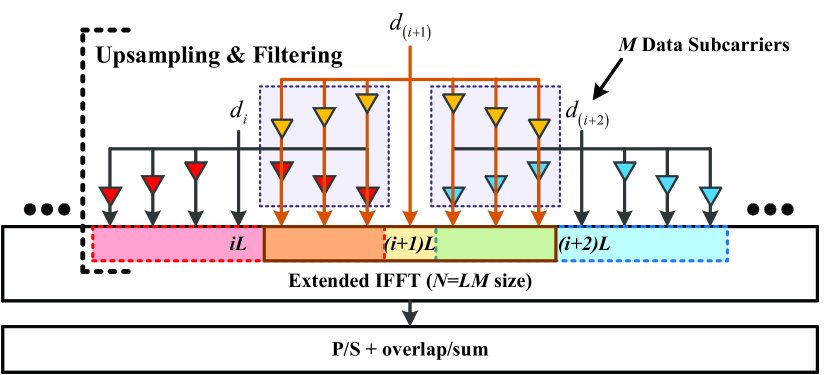
Figure 1: The QAM-FBMC transmitted signal structure ($L=4$).

II System Model of QAM-FBMC Transceiver

In this section, we write the system model of QAM-FBMC to formulate the MMSE criterion of the receiver. As can be seen in [4] and [6], the system model of QAM-FBMC can be written in matrix form as the sum of the overlapped signals. With this existing system model, it is difficult to represent and formulate MMSE criterion. However, in this paper, we change the model to a matrix representation with stacked form of the data vectors contained in the overlap-and-sum structure. At the end of this section, we will represent the QAM-FBMC system model in the form of a simple linear system.

We denote $M$ as a number of subcarriers, $L$ as an overlapping factor for the filtering in the frequency domain, and $N=LM$ as a number of upsampled frequency points, as shown in Fig. 1.

II-A Transmitted Signal Model

To formulate the stacked representation of overlapped transmit signal, we define the $k$-th stacked data symbol vector $\overline{\bf{d}}\left[k\right]$ as follows:

$$\overline{\bf{d}}\left[k\right]={\left[{{\bf{d}}{{\left[{k-L}\right]}^{T}},\cdots,{\bf{d}}{{\left[k\right]}^{T}},\cdots,{\bf{d}}{{\left[{\left({k+L-1}\right)}\right]}^{T}}}\right]^{T}},$$ (1)

where ${{\bf{d}}\left[k\right]}$ is a $k$-th data vector with the $m$-th element, ${d_{m}}\left[k\right]$, which is a QAM data symbol. The $\overline{\bf{d}}\left[k\right]$ includes the $\left({k-L+1}\right)$-th to the $\left({k+L-1}\right)$-th data symbols considering the overlap-and-sum structure, and includes $\left(k-L\right)$-th symbol to consider interference from channel delays.

From the $\overline{\bf{d}}\left[k\right]$, a $k$-th transmitted signal ${\bf{\bar{x}}}\left[k\right]$ in the stacked representation can be written as

$${\bf{\bar{x}}}\left[k\right]={\overline{\bf{G}}_{f}}\overline{\bf{d}}\left[k\right].$$ (2)

And ${\overline{\bf{G}}_{f}}$ is a stacked pulse-shaping filter matrix of size $\left({M+N}\right)\times 2N$ as

$${\overline{\bf{G}}_{f}}=\left[{{\bf{G}}_{f}^{\left({-L}\right)},\cdots,{\bf{G}}_{f}^{\left(0\right)},\cdots,{\bf{G}}_{f}^{\left({L-1}\right)}}\right].$$ (3)

The ${\bf{G}}_{f}^{\left(l\right)}$ is constructed by $m$-th column ${\bf{g}}_{m}^{\left(l\right)}$ with $\left(n+M\right)$-th element $g_{m}^{\left(l\right)}\left[n\right]$, and $g_{m}^{\left(l\right)}\left[n\right]$ is defined in $n=-M,\cdots,N-1$ range as follows:

$$g_{m}^{\left({l\geq 0}\right)}\left[n\right] =\left\{\!\!{\begin{array}[]{*{20}{l}}{p_{0}\left[n\right]{e^{\left({j2\pi\frac{{m\left({n-lM}\right)}}{M}}\right)}}},&{n=lM,\cdots,N-1,}\\ 0,&{{\rm{otherwise,}}}\end{array}}\right.$$ (4)

$$g_{m}^{\left({l<0}\right)}\left[n\right] =\left\{\!\!{\begin{array}[]{*{20}{l}}{p_{0}\left[n\right]{e^{\left({j2\pi\frac{{m\left({n-lM}\right)}}{M}}\right)}}},&{n=-M,\cdots,N+lM-1,}\\ 0,&{{\rm{otherwise,}}}\end{array}}\right.$$

where $p_{0}\left[n\right]$ is a prototype filter defined in $n=0,\cdots,N-1$ range. By equation (2), we can now represent the transmitted signal that has passed the overlap-and-sum structure without sum operation.

II-B Received Signal Model

To represent the time-domain channel for the stacked vector ${\bf{\bar{x}}}\left[k\right]$, we define $\left({N+M}\right)\times\left({N+M}\right)$ channel convolution matrix ${\bf{H}}$, and the each column of the matrix is given by shift of the channel impulse response with $L_{c}$ taps as follows:

$${\left[{\bf{H}}\right]_{\left({{\rm{:,}}}m\right)}}={\rm{shift}}\left\{{{{\left[{{h_{0}}\,\cdots\,{h_{{L_{c}}-1}}\,\,{{\bf{0}}_{N+M-{L_{c}}}}}\right]}^{T}},\,m-1}\right\}.$$ (5)

The $k$-th received signal vector ${\bf{y}}\left[k\right]$ of size $N\times 1$ can be written as

$${\bf{y}}\left[k\right]={\bf{TH}}{\overline{\bf{G}}_{f}}\overline{\bf{d}}\left[k\right]+{\bf{n}}\left[k\right],$$ (6)

where ${\bf{T}}=\left[{{{\bf{0}}_{N\times M}}{\rm{\;\;}}{{\bf{I}}_{N}}}\right]$ is a time-domain slice matrix to extract the samples in the $k$-th received window, and ${\bf{n}}\left[k\right]$ is the additive white Gaussian noise (AWGN) vector with complex Gaussian distribution of $CN\left({{\bf{0}},\sigma_{n}^{2}{{\bf{I}}_{N}}}\right)$. If we simply consider linear receiver process as a filter of size $M\times N$, we can represent the $k$-th detected data symbol as follows:

$${\bf{\tilde{d}}}\left[k\right]={\bf{Q}}_{f}^{H}{{\bf{H}}_{\rm{eff}}}\overline{\bf{d}}\left[k\right]+{\bf{Q}}_{f}^{H}{\bf{n}}\left[k\right],$$ (7)

where ${{\bf{H}}_{\rm{eff}}}={\bf{TH}}{\overline{\bf{G}}_{f}}$, and ${{\bf{Q}}_{f}}$ is a receiver filter matrix that we will formulate by the MMSE criterion in section III. Overall, we show the QAM-FBMC transceiver structure in stacked matrix representation in Fig. 2.

III Receiver Filter by MMSE Criterion

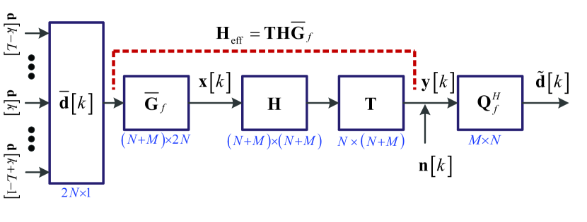
Figure 2: The stacked matrix representation of the QAM-FBMC system.

In this section, we formulate the receiver filter matrix ${{\bf{Q}}_{f}}$ that follows the MMSE criterion. To do this, we set a MMSE problem of the $k$-th detected data symbol as follows:

$${\bf{\hat{Q}}}_{f}^{\left({{\rm{MMSE}}}\right)} =\mathop{\arg\min}\limits_{{{\bf{Q}}_{f}}}E\left[{\left\|{\bf{e}}\right\|_{2}^{2}}\right]=\mathop{\arg\min}\limits_{{{\bf{Q}}_{f}}}E\left[{\left\|{{{\bf{\tilde{d}}}\left[k\right]}-{\bf{S}}\overline{\bf{d}}\left[k\right]}\right\|_{2}^{2}}\right]$$ (8)

$$=\mathop{\arg\min}\limits_{{{\bf{Q}}_{f}}}E\left[{\left\|{\left({{\bf{Q}}_{f}^{H}{{\bf{H}}_{\rm{eff}}}\overline{\bf{d}}\left[k\right]+{\bf{Q}}_{f}^{H}{\bf{n}}}\right)-{\bf{S}}\overline{\bf{d}}\left[k\right]}\right\|_{2}^{2}}\right],$$

where ${\bf{S}}=\left[{{{\bf{0}}_{M\times N}},\cdots,{{\bf{I}}_{M}},\cdots{{\bf{0}}_{M\times\left({L-1}\right)M}}}\right]$ is a matrix for extracting the $k$-th data symbol from the stacked vector ${\overline{\bf{d}}\left[k\right]}$. The expectation of the squared-error becomes

$$E\left\{{\left\|{\bf{e}}\right\|_{2}^{2}}\right\} ={\rm{tr}}\left\{{\left({{\bf{Q}}_{f}^{H}{{\bf{H}}_{{\rm{eff}}}}-{\bf{S}}}\right)\left({{\bf{H}}_{{\rm{eff}}}^{H}{{\bf{Q}}_{f}}-{{\bf{S}}^{H}}}\right)}\right\}\sigma_{d}^{2}$$ (9)

$$+{\rm{tr}}\left\{{{\bf{Q}}_{f}^{H}{{\bf{Q}}_{f}}}\right\}\sigma_{n}^{2},$$

where we assume that the covariance of the stacked data symbol vector is $E\left[{\overline{\bf{d}}{{\overline{\bf{d}}}^{H}}}\right]=\sigma_{d}^{2}{{\bf{I}}_{2N}}$, and the data symbols and AWGN are uncorrelated. We can rewrite the (9) as follows:

$$E\left\{{\left\|{\bf{e}}\right\|_{2}^{2}}\right\}={\rm{tr}}\left\{{{\bf{Q}}_{f}^{H}{\bf{A}}{{\bf{Q}}_{f}}-{\bf{Q}}_{f}^{H}{\bf{B}}-{{\bf{B}}^{H}}{{\bf{Q}}_{f}}+\sigma_{d}^{2}{\bf{I}}}\right\}$$ (10)

$$={\rm{tr}}\left\{{{{\left({{{\bf{C}}^{H}}{{\bf{Q}}_{f}}-{{\bf{C}}^{-1}}{\bf{B}}}\right)}^{H}}\left({{{\bf{C}}^{H}}{{\bf{Q}}_{f}}-{{\bf{C}}^{-1}}{\bf{B}}}\right)+{{\bf{e}}_{\min}}}\right\},$$

where ${\bf{A}}=\sigma_{d}^{2}{{\bf{H}}_{{\rm{eff}}}}{\bf{H}}_{{\rm{eff}}}^{H}+\sigma_{n}^{2}{{\bf{I}}_{N}}$, ${\bf{B}}={{\bf{H}}_{{\rm{eff}}}}{{\bf{S}}^{H}}\sigma_{d}^{2}$, ${\bf{A}}={\bf{C}}{{\bf{C}}^{H}}$ (can be factorized by singular value decomposition), and ${{\bf{e}}_{\min}}=\sigma_{d}^{2}{{\bf{I}}_{2N}}-{{\bf{B}}^{H}}{{\bf{A}}^{-1}}{\bf{B}}$. Since ${{\bf{e}}_{\min}}$ is not related to ${{{\bf{Q}}_{f}}}$, and the left term is the form of Frobenius norm, the equation (10) becomes convex [9]. Therefore, the minimum point is ${{\bf{C}}^{H}}{{\bf{Q}}_{f}}-{{\bf{C}}^{-1}}{\bf{B}}=0$, and the solution of the MMSE problem becomes

$${\bf{\hat{Q}}}_{f}^{\left({{\rm{MMSE}}}\right)}={{\bf{C}}^{-H}}{{\bf{C}}^{-1}}{\bf{B}}={{\bf{A}}^{-1}}{\bf{B}}={\left({{{\bf{H}}_{{\rm{eff}}}}{\bf{H}}_{{\rm{eff}}}^{H}+\frac{{\sigma_{n}^{2}}}{{\sigma_{d}^{2}}}{\bf{I}}}\right)^{-1}}\!\!{{\bf{H}}_{{\rm{eff}}}}{{\bf{S}}^{H}}.$$ (11)

IV Waveform Design with MMSE Receiver

We define the QAM-FBMC waveform design problem as the optimization of the prototype filter. We assume that the single prototype filter for practical transmission structure, and prototype filter is complex modulated by the frequency coefficients as follows:

$${p_{0}}\left(n\right)=\sum\limits_{k=-\left({K-1}\right)}^{K-1}{{q_{k}}{e^{j2\pi\frac{{kn}}{{N}}}}}={q_{0}}+2\sum\limits_{k=1}^{K-1}{{\rm{Re}}\left[{{q_{k}}{e^{j2\pi\frac{{kn}}{{N}}}}}\right]},$$ (12)

where the coefficients are conjugated symmetric as ${q_{k}}=q_{-k}^{*}$, and $K$ is a number of non-zero coefficients in the one-sided frequency domain. Therefore, to design the waveform, we optimize the frequency coefficient vector ${\bf{q}}$ of size $K$ with $k$-th element ${q_{k}}$ $\left({k=0,\cdots,K-1}\right)$.

Before formulating a filter design problem, we need to update the existing average self-signal-to-noise-and-interference ratio (self-SINR) expression in [6] using the stacked representation, and the self-SINR $\Upsilon\left({\sigma_{n}^{2},{{\bf{q}}}}\right)$ can be defined as follows:

$$\Upsilon\left({\sigma_{n}^{2},{\bf{q}}}\right)\!=\!\frac{1}{M}\!\sum\limits_{i=0}^{M-1}\!{\frac{{{{\left|{{{\left[{{\bf{Q}}_{f}^{H}{{\bf{H}}_{{\rm{eff}}}}}\right]}_{\left({i,i+N}\right)}}}\right|}^{2}}}}{{\sum\limits_{j=0\atop j\neq i+N}^{2N-1}{{{\left|{{{\left[{{\bf{Q}}_{f}^{H}{{\bf{H}}_{{\rm{eff}}}}}\right]}_{\left({i,j}\right)}}}\right|}^{2}}}\!+\!{{\left[{{\bf{Q}}_{f}^{H}{{\bf{Q}}_{f}}}\right]}_{\left({i,i}\right)}}\sigma_{n}^{2}}}},$$ (13)

where the receiver filter ${{\bf{Q}}_{f}}$ can be ${{\bf{Q}}_{f}}={\bf{Q}}_{f}^{\left({{\rm{MF}}}\right)}={\bf{TG}}_{f}^{\left(0\right)}$ for matched filter, and ${{\bf{Q}}_{f}}={\bf{\hat{Q}}}_{f}^{\left({{\rm{MMSE}}}\right)}$ for the MMSE filter as shown in (11).

With reference to [6], the optimization problem can be formulated with the spectral and time localization constraints as follows:

$$\mathop{\text{maximize}}\limits_{{{\bf{q}}}} \Upsilon\left({\sigma_{n}^{2},{{\bf{q}}}}\right)$$ (14)

subject to $${\sigma_{t}}<{\epsilon_{t}},\,\,\,\left|{q_{0}}+2\sum\limits_{k=1}^{K-1}{{\rm{Re}}\left[{{q_{k}}}\right]}\right|<{\epsilon_{0}},$$

$$\left|\sum\limits_{k=1}^{K-1}{{k}{\rm{Im}}\left[{{q_{k}}}\right]}\right|<{\epsilon_{1}},\,\,\,\left|\sum\limits_{k=1}^{K-1}{{k^{2}}{\rm{Re}}\left[{{q_{k}}}\right]}\right|<{\epsilon_{2}},$$

where ${\sigma_{t}}$ is a time dispersion parameter defined as

$${\sigma_{t}}=\frac{1}{N}\sqrt{\sum\limits_{n=0}^{N-1}{{{\left({n-\sum\limits_{n=0}^{N-1}{n{{\left|{p_{0}\left[n\right]}\right|}^{2}}}}\right)}^{2}}{{\left|{p_{0}\left[n\right]}\right|}^{2}}}}.$$ (15)

Since the prototype filter problem is non-convex with the high-dimensional variables, thus the filter design may require a high computational complexity. After the prototype filter is successfully designed, the system can simply utilize the designed filter at no extra design cost, however it is very difficult to redesign this filter every time the channel changes. Therefore, this paper assumes that the prototype filter is pre-designed before the transmission. On the other hand, in equation (13), the self-SINR depends on the channel ${\bf{H}}$ and the noise variance of the receiver $\sigma_{n}^{2}$. Since it is difficult to consider an actual channel value or a particular channel model when pre-designing the prototype filter, we assume that the channel is AWGN with ${{\bf{H}}_{{\rm{eff}}}}={\bf{T}}{\overline{\bf{G}}_{f}}$. About the the noise variance of the receiver $\sigma_{n}^{2}$, we set the target signal-to-noise ratio (SNR) to 15, 30, 50, and infinite dB, and design the prototype filter considering the MMSE receiver filter for each target SNR.

Since the optimization problem (14) cannot be solved with convex optimization tool, we design the prototype filters with $K=15$ frequency domain filter taps and $L=4$ oversampling factor through the pattern search algorithm which is a global optimization technique [10]. The pattern search algorithm basically performs a polling process, which updates the optimal point by adding or subtracting each vector element from a given vector point. We set the self-SINR function $\Upsilon\left({\sigma_{n}^{2},{\bf{q}}}\right)$ for the frequency coefficient vector $\bf{q}$ as the fitness function, the fall-off rate conditions as the linear constraint, and the time dispersion condition as the nonlinear constraint. The tolerance parameters of each constraint are set to $\epsilon_{0}=0.01$ and $\epsilon_{1}=\epsilon_{2}=\epsilon_{t}=0.1$.

The design results are described in Table I, and summarized in Table II. The Fig. 3 shows the self-SINR performances of the each prototype filter with SNR variation. As intended in the filter design, the Type G15 and G30 filters exhibit the highest self-SINR at 15dB and 30dB SNR, respectively. Overall, the proposed prototype filters for the MMSE receiver filter show better performances than the reference filters for the matched receiver filter. Specifically, comparing the reference filter Type 2 and Type G30 at the SNR of 30dB, the self-SINR can achieve the performance improvement of 4.25dB, and in the case of 50dB SNR, the Type G50 improves the self-SINR of 5.98dB.

TABLE I: Proposed filter coefficients in the frequency domain

	Type G15	Type G30	Type G50	Type Ginf
	Only real coefficients
$q_{0}$	+1.0000	+1.0000	+1.0000	+1.0000
$q_{1}$	-0.8660	-0.9591	-0.9988	-0.9655
$q_{2}$	+0.6662	+0.7533	+0.7628	+0.7616
$q_{3}$	-0.3932	-0.3915	-0.3597	-0.4422
$q_{4}$	+0.0066	+0.0844	+0.1029	+0.1859
$q_{5}$	+0.2122	+0.2388	+0.1849	+0.0610
$q_{6}$	-0.2680	-0.4369	-0.3509	-0.1987
$q_{7}$	+0.1702	+0.2274	+0.2325	+0.1965
$q_{8}$	-0.0050	-0.0648	-0.1383	-0.1652
$q_{9}$	-0.1571	-0.0774	-0.0504	-0.0025
$q_{10}$	+0.1871	+0.2961	+0.3059	+0.1745
$q_{11}$	-0.0910	-0.2442	-0.2552	-0.1267
$q_{12}$	+0.0091	+0.1152	+0.1836	+0.1106
$q_{13}$	+0.1623	-0.0077	-0.2207	-0.1760
$q_{14}$	-0.1315	-0.0317	+0.1033	+0.0889

TABLE II: Comparison of the prototype filters

	Ref. [4]	Ref. [6]	Proposed
Type	2	C	G15	G30	G50	Ginf
Receiver filter	Matched		MMSE
Target SNR (dB)	$\infty$	$\infty$	15	30	50	$\infty$
$K$(taps)	15	15	15	15	15	15
$\Upsilon\left({0,{\bf{q}}}\right)$ (dB)	19.2	17.4	22.8	24.9	25.4	25.4
Fall-off rate	${\left|\omega\right|^{-4}}$	${\left|\omega\right|^{-5}}$	${\left|\omega\right|^{-5}}$	${\left|\omega\right|^{-5}}$	${\left|\omega\right|^{-5}}$	${\left|\omega\right|^{-5}}$
${\sigma_{t}}$	0.197	0.083	0.077	0.078	0.075	0.064
Coefficient	Complex	Real	Real	Real	Real	Real

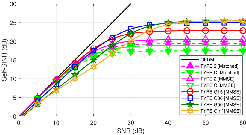
Figure 3: The self-SINR comparisons of the designed prototype filters with SNR variation.

V Simulation Results

In this section, we compare the performances of the designed prototype filters, which are presented in Table II. For reference filters with matched receiver filter, we use a single-tap MMSE equalizer in the upsampled frequency domain. Also, we consider the performances of the reference filters with MMSE receiver filter, which is same as the process of the proposed prototype filter.

The common simulation parameters are $L=4$, $M=128$, $\sigma_{d}^{2}=1$, 16-QAM/64-QAM, 2GHz carrier frequency, and 15kHz subcarrier spacing. The channel models of the simulation are AWGN, extended ITU pedestrian A (EPA), and extended ITU vehicular A (EVA) [11].

In Fig. 4, 5, and 6, we compare the probability of bit error (BER) performances between the reference filters with matched receiver filter and the proposed filters with the MMSE receiver filter. In the simulation, as mentioned above, we can see that the prototype filters with higher self-SINR show better BER performances as expected, and the performances of the proposed filters are significantly enhanced than the reference filters. As shown in Fig. 4, the Type G30 filter with the highest self-SINR at 30dB SNR shows the best performance in AWGN. And in EPA and EVA channels which require higher SNR, Type G50 and GInf show slightly better BER performances than Type G30. Overall, we can expect that the Type G30 filter performs well in most of the scenarios, so we expect it to be usable in general situation. Additionally, we check the BER performances of the reference filters with MMSE receiver filter. Even if the signal with the reference filters is received through MMSE filter, the reference filters show the slightly better performances than the matched receiver, but still worse than the proposed filter because it is not designed to use the MMSE filter.

The most important part in these BER performance results is that the performance degradation of the reference filter compared to OFDM can be significantly mitigated through the proposed prototype filter and MMSE receive structure. Specifically, by the proposed filter and receiver, we can reduce the residual interference so that QAM-FBMC can achieve $10^{-5}$ uncoded BER performance in high modulation order. In particular, this MMSE receiver works in the linear system instead of complex nonlinear operations such as successive cancellation, and it can be realizable when QAM-FBMC is used in a realistic environment.

Additionally, we can confirm that the designed prototype filters assuming AWGN channel show almost the same performance trends as for AWGN, even if BER simulations are performed on the fading channel models. In the practical system, if the QAM-FBMC transmitter knows or predicts the received SNR, the system can use the pre-designed prototype filters corresponding to the target SNR, which may exhibit the best BER performance. Therefore, if the QAM-FBMC system utilizes the pre-designed prototype filters appropriately, we can expect the good performance even considering the practical channel and varying SNR at the receiver.

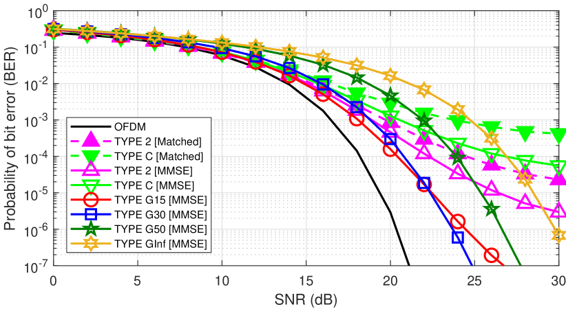
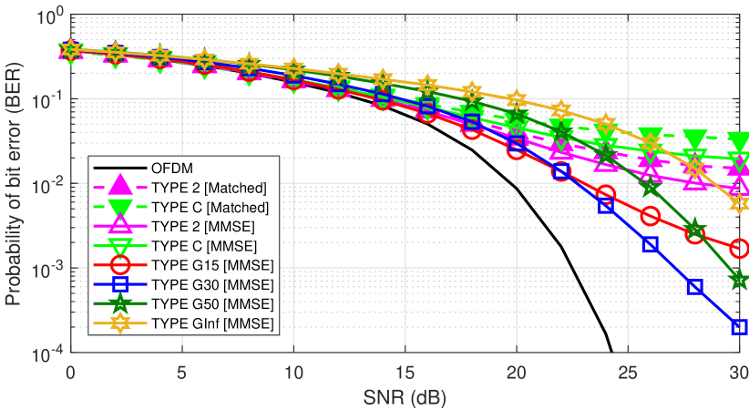
Figure 4: The BER performance comparisons in the AWGN channel with 16-QAM (top) and 64-QAM (bottom).

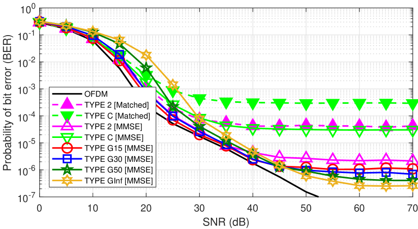
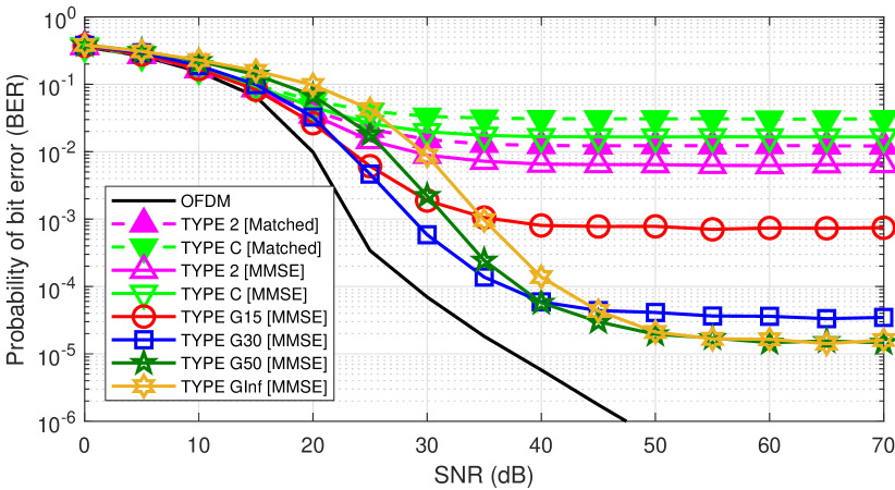
Figure 5: The BER performance comparisons in the EPA channel with 16-QAM (top) and 64-QAM (bottom).

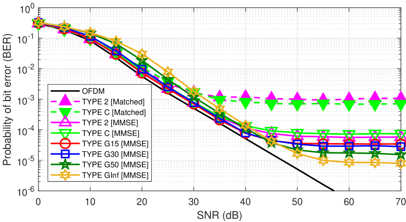
Figure 6: The BER performance comparisons in the EVA channel with 16-QAM (top) and 64-QAM (bottom).

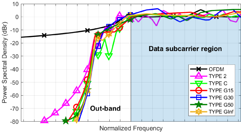
Figure 7: The comparison of power spectral density between OFDM and various QAM-FBMC prototype filters.

Fig. 7 shows the power spectral density (PSD) of the prototype filters for comparing the spectral confinement characteristics. As we can expect from Table II, the Type C and the proposed filters all show the almost same PSD, with a good spectral confinement of ${\left|\omega\right|^{-5}}$, the Type 2 has a medium spectral confinement with a fall-off rate of ${\left|\omega\right|^{-4}}$, and OFDM shows the worst characteristic.

VI Conclusions

In this paper, we designed waveforms for QAM-FBMC considering an MMSE receiver filter. In a QAM-FBMC system using a non-orthogonal pulse-shaping filter, the conventional matched receiver filter cannot be optimal, and we proposed a MMSE filter to minimize interference. In that regard, we simplified the linear system model for QAM-FBMC using stacked vectorization, and formulated a receiver filter following the MMSE criterion. In addition, we designed prototype filters that had a superior self-SINR under the condition of the linear receiver. Finally, we confirmed that the proposed filters show the best performance with the design intent through simulation results. In addition, the formulations of the linear system and self-SINR equations for QAM-FBMC showed the simpler representation than that of the previously complex QAM-FBMC system, therefore, we identified the possibility of applying popular signal processing technology directly to QAM-FBMC in the future.

References

- [1] P. Banelli, S. Buzzi, G. Colavolpe, A. Modenini, F. Rusek, and A. Ugolini, “Modulation formats and waveforms for 5G networks: Who will be the heir of OFDM?: An overview of alternative modulation schemes for improved spectral efficiency,” IEEE Signal Processing Magazine, vol. 31, no. 6, pp. 80–93, Nov 2014.
- [2] M. Bellanger, D. Le Ruyet, D. Roviras, M. Terré, J. Nossek, L. Baltar, Q. Bai, D. Waldhauser, M. Renfors, T. Ihalainen et al., “FBMC physical layer: a primer,” PHYDYAS, 2010.
- [3] R. Zakaria and D. Le Ruyet, “A novel filter-bank multicarrier scheme to mitigate the intrinsic interference: application to MIMO systems,” IEEE Trans. Wireless Commun., vol. 11, no. 3, pp. 1112–1123, 2012.
- [4] Y. H. Yun, C. Kim, K. Kim, Z. Ho, B. Lee, and J.-Y. Seol, “A new waveform enabling enhanced QAM-FBMC systems,” in Proc. IEEE SPAWC, 2015, pp. 116–120.
- [5] C. Kim, Y. H. Yun, K. Kim, and J. Seol, “Introduction to QAM-FBMC: From waveform optimization to system design,” IEEE Communications Magazine, vol. 54, no. 11, pp. 66–73, November 2016.
- [6] H. Kim, H. Han, and H. Park, “Waveform design for QAM-FBMC systems,” in 2017 IEEE 18th International Workshop on Signal Processing Advances in Wireless Communications (SPAWC), July 2017, pp. 1–5.
- [7] H. Han and H. Park, “Design on the waveform for qam-fbmc system in the presence of residual cfo,” in 2019 16th IEEE Annual Consumer Communications Networking Conference (CCNC), Jan 2019, pp. 1–2.
- [8] H. V. Poor, An introduction to signal detection and estimation. Springer Science & Business Media, 2013.
- [9] S. Boyd and L. Vandenberghe, Convex optimization. Cambridge university press, 2004.
- [10] C. Audet and J. E. Dennis Jr, “A pattern search filter method for nonlinear programming without derivatives,” SIAM Journal on Optimization, vol. 14, no. 4, pp. 980–1010, 2004.
- [11] 3GPP, “Evolved Universal Terrestrial Radio Access (E-UTRA); User Equipment (UE) radio transmission and reception,” 2008.