Cominetti et al.

Approximation and Convergence of Large Atomic Congestion Games

Approximation and Convergence of Large Atomic Congestion Games

Roberto Cominetti Facultad de Ingeniería y Ciencias, Universidad Adolfo Ibáñez, Santiago, Chile, roberto.cominetti@uai.cl, https://sites.google.com/site/cominettiroberto Marco Scarsini Dipartimento di Economia e Finanza, Luiss University, Roma, Italy, marco.scarsini@luiss.it, https://sites.google.com/view/marcoscarsini Marc Schröder School of Business and Economics, Maastricht University, Maastricht, The Netherlands, m.schroder@maastrichtuniversity.nl, https://www.maastrichtuniversity.nl/p70024063 Nicolás Stier-Moses Core Data Science, Meta, Menlo Park, USA, nicostier@yahoo.com, https://sites.google.com/site/nicostier

We consider the question of whether, and in what sense, Wardrop equilibria provide a good approximation for Nash equilibria in atomic unsplittable congestion games with a large number of small players. We examine two different definitions of small players. In the first setting, we consider games where each player’s weight is small. We prove that when the number of players goes to infinity and their weights to zero, the random flows in all (mixed) Nash equilibria for the finite games converge in distribution to the set of Wardrop equilibria of the corresponding nonatomic limit game. In the second setting, we consider an increasing number of players with a unit weight that participate in the game with a decreasingly small probability. In this case, the Nash equilibrium flows converge in total variation towards Poisson random variables whose expected values are Wardrop equilibria of a different nonatomic game with suitably-defined costs. The latter can be viewed as symmetric equilibria in a Poisson game in the sense of Myerson, establishing a plausible connection between the Wardrop model for routing games and the stochastic fluctuations observed in real traffic. In both settings we provide explicit approximation bounds, and we study the convergence of the price of anarchy. Beyond the case of congestion games, we prove a general result on the convergence of large games with random players towards Poisson games.

unsplittable atomic congestion games; nonatomic congestion games; Wardrop equilibrium; Poisson games; symmetric equilibrium; price of anarchy; price of stability; total variation Primary: 91A14; secondary: 91A07, 91A43, 60B10 Primary: Games/group decisions: non-atomic; secondary: Networks/graphs: multicommodity

1 Introduction

Nonatomic congestion games were introduced by Wardrop [63] as a model for traffic networks with many drivers, where each single agent has a negligible impact on congestion. The model was stated in terms of continuous flows, which are easier to analyze compared to a discrete model with a finite but large number of players. The heuristic justification is that a continuous flow model is a natural approximation to a game with many players, each one having a negligible weight. Although this argument is intuitive and plausible, the question of whether nonatomic games are the limit of atomic games has only been formally addressed in special cases, mainly for atomic splittable games with homogeneous players as in Haurie and Marcotte [29].

Motivated by applications such as road traffic and telecommunications, it is also important to consider the issue of approximating unsplittable routing games. In them, players must route a given load over a single path, which can be chosen either deterministically or at random using a mixed strategy. We consider the more general class of atomic unsplittable congestion games (not necessarily routing games) and allow for heterogeneous players. The main question we address is whether Nash equilibria for these games are well approximated by a Wardrop equilibrium of a limiting nonatomic congestion game. A convergence result would provide a stronger support for Wardrop’s model as an approximation for large games with many small players, especially if we can estimate the distance between the corresponding equilibrium solutions.

In a weighted congestion game, there is a finite number of players who are characterized by a type and a weight. The type determines the set of feasible strategies for the player and the weight determines the player’s impact on the costs. Moreover, there is a finite set of resources and each strategy corresponds to a subset of these resources. Players of a given type have the same set of available strategies. A strategy profile for all players induces a flow on each strategy equal to the total weight of players choosing it, as well as a load on each resource equal to the total weight of players using that resource as part of their strategy. The cost of using a resource is a weakly increasing function of its load, and the cost of a strategy is additive over its resources. This defines a finite cost-minimization game. As shown by Rosenthal [53], every congestion game in which all the players have the same weight admits a potential and has equilibria in pure strategies. With heterogeneous weights, only mixed equilibria are guaranteed to exist [46].

As a special case of congestion games, a routing game features a finite directed network whose edges represent the resources. The origin-destination pairs encode the types, and the corresponding origin-destination paths provide the strategies. To illustrate, consider a routing game over a simple network composed of two parallel edges with the same strictly-increasing cost function $c(\,\cdot\,)$, as shown in Figure 1, and suppose that there are $n$ players who need to choose an edge to route an identical weight of $w\equiv d/n$. Here, $d$ denotes the total weight or demand.

Figure 1: Parallel edge network.

In a symmetric equilibrium every player randomizes by choosing each route with probability $1/2$. Consequently, the number of players on each route is distributed as a $\operatorname{\mathsf{Binomial}}(n,1/2)$ random variable. The total load on each edge is therefore $d/n$ times a $\operatorname{\mathsf{Binomial}}(n,1/2)$, and converges in distribution to $d/2$, which is precisely the Wardrop equilibrium for a total demand of $d$ units of flow. Note that already in this simple example there is a multitude of other equilibria where $n_{1}$ and $n_{2}$ players, respectively, choose the upper and lower edges for sure (with $n_{1},n_{2}\leq n/2$), and the remaining players (if any) randomize appropriately so as to equalize the expected cost of both routes. This includes the special case of a pure equilibrium in which half of the players take each route, up to one unit if $n$ is odd. As the number of players $n$ tends to infinity, all these different equilibria converge to the unique Wardrop equilibrium with a $(d/2,d/2)$-split of the flow.

In real networks, players are confronted to make decisions while facing multiple sources of uncertainty. In particular, even if the population of potential drivers might be known, the subset of drivers that are actually on the road at any given time is random. In fact, the contribution of an additional car to congestion is small but not negligible, and the congestion experienced by an agent depends basically on how many drivers are on the road at the same time. To that point, Angelidakis et al. [3] and Cominetti et al. [17] studied Bernoulli congestion games in which players participate with an independent probability. If we focus on a small time interval, the probability that any given player participates in the game during that interval emerges naturally as a small parameter. Motivated by this model, we ask the question whether a congestion game with a large but random number of players and small participation probabilities can be approximated by a nonatomic congestion game. To address this question we study the convergence of the Nash equilibria for a sequence of Bernoulli games towards the Wardrop equilibria of some nonatomic game. Taking the limit in this setting yields a different limit game in which the random loads on the resources converge to a family of Poisson random variables, whose expected values can be again characterized as Wardrop equilibria of a suitably defined nonatomic game or, alternatively, as an equilibrium of a Poisson game in the sense of Myerson [43]. This establishes a novel and precise connection between the Wardrop model and Poisson games. To provide some insight, consider again the parallel-edge example of Figure 1, except that now each of the $n$ players has a unit weight, but is present in the game with a small probability $d/n$. In this case the effective demand is a random variable $D^{n}\sim\operatorname{\mathsf{Binomial}}(n,d/n)$, which converges as $n\to\infty$ to a random variable $D\sim\operatorname{\mathsf{Poisson}}(d)$. Also, in a symmetric equilibrium where each player choses an edge uniformly at random, the load on each route is distributed as a $\operatorname{\mathsf{Binomial}}(n,d/(2n))$ and converges to a $\operatorname{\mathsf{Poisson}}(d/2)$, whose expected value is again $d/2$. We will show that this convergence holds for all Nash equilibria and for general congestion games with an increasing number of heterogenous players who are active with different vanishing probabilities.

Note that in both cases—vanishing weights and vanishing probabilities—the equilibria of the nonatomic limit games characterize the expected values of the random loads. However, in the Poisson regime the resource loads remain random in the limit, whereas in the Wardrop limit these random loads converge to a constant. The fact that the Poisson limit retains some variability makes it more suitable to model the traffic flows observed in real networks. As a matter of fact, real traffic flows exhibit stochastic fluctuations that have been empirically confirmed to be close to Poisson distributions, at least under moderate congestion conditions. As an illustration, Figure 2 shows the histograms of traffic counts over three consecutive 10 minute intervals, observed every Thursday during 2 years on a specific road segment in Dublin. The red curves give the expected counts for Poisson distributions with the same mean. These histograms reveal a persistent day-to-day variability of traffic flows, so that a model predicting a random distribution is one step closer to reality compared to the point estimates provided by Wardrop equilibrium. Our results establish a theoretically sound connection between the Wardrop and Poisson equilibria, which, combined, seem to provide a more sensible model for the traffic flows observed in real networks.

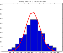
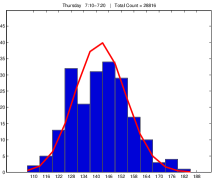
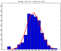
Figure 2: Traffic counts. Dublin 2017-2018, Thursday 7:00-7:30 AM. Data from Transport Infrastructure Ireland. https://www.tii.ie/roads-tolling/operations-and-maintenance/traffic-count-data/

1.1 Our Contribution

After introducing the relevant classes of congestion games in Section 2, Section 3 deals with nonatomic approximations of weighted atomic congestion games. Under mild and natural conditions we show that Nash equilibria in a sequence of weighted congestion games converge to a Wardrop equilibrium of a limiting nonatomic game. More precisely, if the number of players grows to infinity and their weights tend to zero in a way that the aggregate demands converge, then, for any sequence of mixed equilibria in the finite games, the random variables that represent the resource loads converge in distribution to a (deterministic) Wardrop equilibrium for a nonatomic limit game. We stress that players are not assumed to be symmetric and that they may have different weights and strategy sets. As long as their weights converge to zero, the random resource loads converge in distribution to some constants, which are precisely a Wardrop equilibrium for the limit game. This provides a strong support to Wardrop’s model as a sensible approximation for large unsplittable congestion games with many small players.

Section 4 focuses on approximations of Bernoulli congestion games. It considers sequences of Bayesian Nash equilibria for Bernoulli congestion games when the participation probability of players tends to zero, and establishes the convergence of the resource loads towards a family of Poisson variables whose expected values are Wardrop equilibria of another nonatomic game with suitably defined costs. In Section 5 we unveil the connection between this nonatomic limit game and a Poisson game in the sense of Myerson [43], namely, the Wardrop equilibria are in one-to-one correspondence with the equilibria of an associated Poisson game with countably many players and demands distributed as Poisson random variables. We stress that Poisson games were originally introduced axiomatically and not as a limit of a sequence of finite games. We close this gap by proving a general result on convergence of sequences of games with Bernoulli players (not necessarily congestion games) towards Poisson games. This constitutes a novel alternative justification for Poisson games.

In Section 6 we derive non-asymptotic bounds for the distance between the distributions of the equilibrium loads in the finite games and the Wardrop and Poisson counterparts. These bounds provide explicit estimates for using these simpler models to approximate the equilibria in the finite games. Finally, in Section 7 we turn to investigate the convergence of the price of anarchy (PoA) and the price of stability (PoS)—as measures of the inefficiency of equilibria—for sequences of weighted congestion games and Bernoulli congestion games.

In summary, the main contributions of this paper are:

1. A formal statement and proof of the fact that Nash equilibria of weighted atomic unsplittable congestion games converge to Wardrop equilibria of nonatomic congestion games, as the weights of all players vanish. This is achieved under very weak conditions and holds even when weights are different (in that case pure Nash equilibria may not exist).

2. A formal statement and proof of the fact that, as the participation probability of each player vanishes, the random loads in Bayesian Nash equilibria of Bernoulli congestion games converge to Poisson random variables whose expectations are Wardrop equilibria of a suitably defined nonatomic congestion game. Again, this is achieved under weak conditions; for instance, the participation probability of different players may differ.

3. A connection between Poisson and Wardrop equilibria for congestion games, and a formal asymptotic justification of Poisson games as limits of Bernoulli games.

4. Non-asymptotic bounds for the distance between the equilibria in weighted and Bernoulli congestion games to the corresponding Wardrop and Poisson equilibria.

5. A proof of the convergence of the PoA and PoS for sequences of weighted and Bernoulli congestion games.

1.2 Related Literature

Convergence of weighted congestion games towards nonatomic games has been considered before, mainly for the case in which players can split their weight over the available strategies. Haurie and Marcotte [29] were the first to study such convergence issues. In a setting of atomic routing games with splittable flows and elastic demands, they proved that when players on each origin-destination (OD) pair are identically replicated $n$ times, in the limit when $n$ grows, the splittable equilibria converge towards Wardrop equilibria. More recently, Jacquot and Wan [30] considered splittable routing on parallel networks with heterogenous players, and Jacquot and Wan [31] studied the approximation of nonatomic aggregative games by a sequence of finite splittable games. Also the relation between Nash equilibria and a Wardrop-like notion of equilibrium in aggregative games with finitely many players, was studied by Paccagnan et al. [50].

We are not aware of any results on convergence of equilibria for unsplittable weighted congestion games. The closest is Milchtaich [38] who studied limits of finite crowding games with an increasing number of players $n$ with identical weights $1/n$, i.e., unweighted congestion games with singleton strategies and type-dependent costs. Considering pure equilibria only, he established the convergence of the per-type aggregate strategy loads towards an equilibrium of a large crowding game. In another related result, Sandholm [57] proved that infinite potential games can be obtained as limits of finite potential games. His results are related to ours because every unweighted congestion game is a potential game [53] and, conversely, every finite potential game is isomorphic to an unweighted congestion game [41]. The difference is that here we consider the more general class of weighted congestion games, which in general do not have a potential structure. Moreover, Sandholm studied only the convergence of the potential functions but did not address the convergence of equilibria. We also mention Feldman et al. [22], who established asymptotic upper bounds for the PoA in unsplittable games when the number $n$ of players increases and their weight is $1/n$. Their results are based on the so-called $(\lambda,\mu)$-smoothness in the large which provides upper bounds for the PoA, but again without addressing the convergence of equilibria. On a similar vein, Chen et al. [15] considered nonatomic congestion games as limits of atomic unsplittable games, in order to define altruism and to investigate its impact on the price of anarchy.

In the present paper we consider unsplittable weighted congestion games and present approximation results for the flows themselves, which is a stronger statement and therefore technically harder to accomplish. In fact, whereas equilibria for splittable congestion games (as well as pure equilibria in the unsplittable case) are conveniently described in terms of flows and loads that live in the same finite dimensional space as Wardrop equilibria, in the unsplittable case with equilibria in mixed strategies these flows and loads become random so that limits must be properly understood in terms of convergence of random variables. This can be used later to derive the convergence of aggregate metrics such as the PoA.

Besides routing games, auctions are another class of games where there is significant previous work on asymptotic properties when the number of players becomes large. Satterthwaite and Williams [58] and Rustichini et al. [56] studied the efficiency loss in markets as the number of bidders grows. Caserta and de Vries [14], Lambert and Shoham [34], Blumrosen and Holenstein [9], Fibich and Gavious [23] used asymptotic analysis to understand the convergence of revenue in various auctions settings. Like our work, several of these references compute equilibria or approximate equilibria as the auctions become larger, and use those characterizations to derive limiting results. Although convergence might appear natural at first sight, some asymptotic results are fragile and only hold under carefully stated assumptions. For instance, Roberts and Postlewaite [52] showed that the gain from deviating from competitive behavior in an exchange economy does not need to diminish as the number of agents in the economy goes to infinity. Also Swinkels [61] and Feldman et al. [22] showed that the inefficiency in auctions does not need to disappear in the limit with a large number of objects and players.

Several old papers considered the stochastic aspects of traffic, both theoretically and empirically, including the role of the Poisson distribution for modeling it [see, e.g., 1, 36, 49, 11, 12, 13, 40]. More recently, various authors have studied congestion games with stochastic features, focusing on the efficiency of equilibria under incomplete information. For instance, Gairing et al. [25] studied the inefficiency of equilibria for congestion games in which the weight of a player is private information. Looking at the cost uncertainty, Nikolova and Stier-Moses [47] and Piliouras et al. [51] considered players’ risk attitudes in the nonatomic and atomic cases, respectively. Roughgarden [55] showed that whenever player types are independent, the inefficiency bounds for complete information games extend to Bayesian Nash equilibria of the incomplete information game. Wang et al. [62] and Correa et al. [18] looked at similar questions for nonatomic routing games. This trend does not only include congestion games: Stidham [60] studied the efficiency of some classical queueing models on various networks, whereas Hassin et al. [28] examined a queueing model with heterogeneous agents and studied how the inefficiency of equilibria varies with the intensity function. Closer to our results on Bernoulli games, Angelidakis et al. [3] considered congestion games with stochastic players who are risk-averse, restricting their attention to the case of parallel edges. In the same spirit, Cominetti et al. [17] studied Bernoulli congestion games, where each player $i$ takes part in the game independently with probability $p_{i}$, and found sharp bounds for the PoA as a function of the maximum $p_{i}$.

Games with a random number of players were introduced by Myerson [42, 43, 44, 45], with the main goal of analyzing elections with a large number of voters. In his seminal paper, Myerson [43] showed that the case where the number of players has a Poisson distribution is of particular relevance, being the only case where an environmental equivalence holds, i.e., the belief of a player of any type about the type profile of the other active players coincides with the belief of an external game theorist. Myerson [44] dealt with large Poisson games in which the parameter of the Poisson distribution diverges. His approach differs from ours in the sense that he starts with a Poisson distribution, axiomatically justified, and lets the expectation of this distribution go to infinity. In our case we start with a finite number of players and let their number diverge in such a way that in the limit we get a Poisson distribution, but not necessarily with a large parameter. Our derivation of Poisson games as limits of finite Bernoulli games seems to be new. The asymptotic approach we take to Poisson games is based on results from Poisson approximation theory. In probability, results about this topic abound. For an overview of this literature, we refer the reader to the books and surveys by Barbour et al. [6], Barbour and Chen [4], Novak [48].

Several other papers have studied the properties of games with random number of players and Poisson games in particular. Among them, Milchtaich [39] provided a sophisticated analysis of general games with population uncertainty. De Sinopoli and Pimienta [20], De Sinopoli et al. [19], Meroni and Pimienta [37] dealt with various properties of equilibria in Poisson games, such as stability and existence of equilibria in undominated strategies. Other papers apply Poisson games in different settings, not necessarily related to elections. Lim and Matros [35] studied contests with finitely many players, where each player takes part in the game independently with the same probability, whereas Du and Gong [21] used a Poisson game to model parking congestion and proposed a decentralized and coordinated online parking mechanism to reduce congestion. Let us finally mention Kordonis and Papavassilopoulos [32] and Bernhard and Deschamps [8] who studied dynamic games where players arrive at random over time.

1.3 Organization of the Paper

The paper is organized as follows. Section 2 describes the different versions of the congestion games that we will study, and introduces the basic notation. Sections 3 and 4 study the convergence of sequences of weighted congestion games and Bernoulli congestion games respectively. Section 5 examines Poisson games in greater generality and focuses on convergence to them. Section 6 provides the non-asymptotic bounds on the rate of convergence of the finite congestion games to their limits, followed by Section 7 where we present convergence results for the PoA and the PoS. Section 8 presents some conclusions and possible directions for future work. Appendices 10 and 9 include auxiliary results and proofs used in Sections 7 and 6 respectively, whereas Appendix 11 provides a short summary of known results on Poisson approximations for sums of Bernoulli random variables that are used to derive our results. Finally, Appendix 12 contains a glossary of notations for ease of reference.

2 Congestion Games: Definitions and Notations

This section introduces the basic models of congestion games and the variations that will be studied in this paper. Informally, a congestion game is played over a set of resources whose costs depend on the mass of players using the resource. Each player chooses a subset of resources among the allowed subsets, seeking to achieve the minimum possible cost. Throughout this paper we consider a finite set of resources $\mathscr{E}$, where each $e\in\mathscr{E}$ is associated with a weakly increasing continuous cost function $c_{e}:\mathbb{N}_{+}\to\mathbb{N}_{+}$. We also fix a finite set of types $\mathscr{T}$ where each type $t\in\mathscr{T}$ is associated with a set of feasible actions $\mathscr{S}_{t}\subseteq 2^{\mathscr{E}}$, which describes the pure strategies.

To name a standard example of a congestion game, routing games capture the topology of a network structure. These games are defined over the set of edges of a finite graph, encoded by $\mathscr{E}$, and the set of OD pairs, encoded by $\mathscr{T}$. The set of actions $\mathscr{S}_{t}$ contains the feasible paths for the OD pair representing type $t$, and the costs $c_{e}(\,\cdot\,)$ represent the delays when traversing an edge $e$.

The structural objects

$$\mathscr{G}=(\mathscr{E},(c_{e})_{e\in\mathscr{E}},\mathscr{T},(\mathscr{S}_{t})_{t\in\mathscr{T}})$$ (1)

will be the same in all the congestion games considered hereafter, and the only differences will be in how we describe the set of players and their behavior. In the nonatomic framework, players are considered to be infinitesimally small and the model is stated in terms of the aggregate mass of players that use each strategy and resource. In contrast, for weighted congestion games, as well as for Bernoulli congestion games, we have a finite set of players who behave strategically. The rest of this section describes these three different models precisely.

As a guide for the notation used in the sequel, we write $\bigtriangleup(\mathscr{S}_{t})$ for the simplex of all probability distributions over the strategy set $\mathscr{S}_{t}$. We use capital letters for random variables and lower case for their expected values. For instance, $X_{e}$ will represent a random load on a resource $e\in\mathscr{E}$ with expected value $x_{e}=\operatorname{\mathsf{E}}[X_{e}]$, and we will add a hat $\widehat{x}_{e}$ when referring to an equilibrium.

2.1 Nonatomic Congestion Games

A nonatomic congestion game $\Gamma^{\infty}$ is given by a pair $(\mathscr{G},\boldsymbol{d})$, where $\mathscr{G}$ stands for the structural objects of the game as in (1), and $\boldsymbol{d}=(d_{t})_{t\in\mathscr{T}}$ is a vector of demands with $d_{t}\geq 0$ representing the aggregate demand of type $t$. The total demand is given by the sum over all types $d_{\operatorname{tot}}=\sum_{t\in\mathscr{T}}d_{t}$.

Each demand $d_{t}$ is split over the corresponding strategies $\mathscr{S}_{t}$ and induces loads on the resources. Specifically, a strategy flow vector $\boldsymbol{y}\coloneqq(y_{t,s})_{t\in\mathscr{T},s\in\mathscr{S}_{t}}$ and a resource load vector $\boldsymbol{x}\coloneqq(x_{e})_{e\in\mathscr{E}}$ are called feasible if they satisfy the following constraints:

$$\forall t\in\mathscr{T},\quad d_{t}=\sum_{s\in\mathscr{S}_{t}}y_{t,s}\text{ with $y_{t,s}\geq 0,\quad$ and }\quad\forall e\in\mathscr{E},\quad x_{e}=\sum_{t\in\mathscr{T}}\sum_{s\in\mathscr{S}_{t}}y_{t,s}\mathds{1}_{\{e\in s\}}.$$ (2)

The set of such feasible flow-load pairs $(\boldsymbol{y},\boldsymbol{x})$ is denoted by $\mathscr{F}(\boldsymbol{d})$. Note that the resource loads $\boldsymbol{x}$ are uniquely defined by the strategy flows $\boldsymbol{y}$, but not vice versa. Nevertheless, instead of only considering strategy flows, we will refer to flow-load pairs because some concepts are easier to express in terms of flows whereas others are defined in terms of loads. The notation and nomenclature is inspired by routing games, and most of our examples will be of this type because they are intuitive and well-studied. However, we will use these terms in the more general setting of congestion games, even when there is no network structure of resources and strategies.

A Wardrop equilibrium is defined as a feasible flow-load pair $(\widehat{\boldsymbol{y}},\widehat{\boldsymbol{x}})\in\mathscr{F}(\boldsymbol{d})$ for which the prevailing cost of all used strategies is minimal, or, mathematically,

$$\forall t\in\mathscr{T},\ \forall s,s^{\prime}\in\mathscr{S}_{t}\quad\widehat{y}_{t,s}>0\implies\sum_{e\in s}c_{e}(\widehat{x}_{e})\leq\sum_{e\in s^{\prime}}c_{e}(\widehat{x}_{e}).$$ (3)

Because only strategies with minimum cost are used, all the strategies used by any given type have the same cost and, as a consequence, any strategy flow decomposition of $\widehat{\boldsymbol{x}}$ yields an equilibrium. The set of Wardrop equilibria of the nonatomic game $\Gamma^{\infty}$ will be denoted by $\operatorname{\mathsf{WE}}(\Gamma^{\infty})$.

2.2 Weighted Congestion Games

A weighted congestion game is defined as a tuple $\Gamma_{{\scriptscriptstyle\operatorname{\mathsf{W}}}}=(\mathscr{G},(w_{i},t_{i})_{i\in\mathscr{N}})$, where $\mathscr{N}$ is a finite set of players and each player $i\in\mathscr{N}$ has a weight $w_{i}\in\mathbb{N}_{+}$ and a type $t_{i}\in\mathscr{T}$ that determines her strategy set $\mathscr{S}_{t_{i}}$. Our use of the term “type” slightly differs from what is common in game theory, where a type is a random variable associated to each player, whose distribution is common knowledge but whose realization is private information. Here, the players’ types are deterministic and the type of each player is common knowledge.

The aggregate demand for each type $t$ and the total demand are given by

$$d_{t}=\sum_{i\colon t_{i}=t}w_{i},\text{\quad and \quad}d_{\operatorname{tot}}=\sum_{t\in\mathscr{T}}d_{t}=\sum_{i\in\mathscr{N}}w_{i}.$$ (4)

Let $\boldsymbol{\sigma}=(\sigma_{i})_{i\in\mathscr{N}}$ be a mixed strategy profile, where $\sigma_{i}\in\bigtriangleup(\mathscr{S}_{t_{i}})$ represents the mixed strategy used by player $i\in\mathscr{N}$, and let $\Sigma\coloneqq\times_{i\in\mathscr{N}}\bigtriangleup(\mathscr{S}_{t_{i}})$ be the set of mixed strategy profiles. Call $\operatorname{\mathsf{E}}_{\boldsymbol{\sigma}}$ the expectation with respect to the product probability measure $\operatorname{\mathsf{P}}_{\boldsymbol{\sigma}}\coloneqq\times_{i\in\mathscr{N}}\sigma_{i}$ over the set of pure strategy profiles $\mathscr{S}=\times_{i\in\mathscr{N}}\mathscr{S}_{t_{i}}$. If $S_{i}$ is the random strategy of player $i$, whose distribution is $\sigma_{i}$, then the probability that player $i$ uses a given resource $e$ is

$$\sigma_{i,e}\coloneqq\operatorname{\mathsf{P}}_{\boldsymbol{\sigma}}(e\in S_{i})=\sum_{s\in\mathscr{S}_{t_{i}}}\sigma_{i}(s)\mathds{1}_{\{e\in s\}}.$$ (5)

Accordingly, the strategy flows $Y_{t,s}$ and the resource loads $X_{e}$ become random variables

$$Y_{t,s}=\sum_{i\colon t_{i}=t}w_{i}\mathds{1}_{\{S_{i}=s\}}\text{\quad and \quad}X_{e}=\sum_{i\in\mathscr{N}}w_{i}\mathds{1}_{\{e\in S_{i}\}},$$ (6)

given by the random realizations of $S_{i}$. Their expected values are

$$y_{t,s}\coloneqq\operatorname{\mathsf{E}}_{\boldsymbol{\sigma}}[Y_{t,s}]=\sum_{i\colon t_{i}=t}w_{i}\sigma_{i}(s)\text{\quad and \quad}x_{e}\coloneqq\operatorname{\mathsf{E}}_{\boldsymbol{\sigma}}[X_{e}]=\sum_{i\in\mathscr{N}}w_{i}\sigma_{i,e}.$$

A straightforward calculation shows that the pair $(\boldsymbol{y},\boldsymbol{x})$ satisfies (2), so that $(\boldsymbol{y},\boldsymbol{x})\in\mathscr{F}(\boldsymbol{d})$.

To take the perspective of a fixed player $i$, we assume the player already selected resource $e$ and define the conditional load

$$X_{i,e}\coloneqq w_{i}+\sum_{j\neq i}w_{j}\mathds{1}_{\{e\in S_{j}\}}.$$ (7)

Using this, the expected cost of player $i$ conditional on the player using the resource $e$ is

$$\operatorname{\mathsf{E}}_{\boldsymbol{\sigma}}[c_{e}(X_{e})\mid e\in S_{i}]=\operatorname{\mathsf{E}}_{\boldsymbol{\sigma}}[c_{e}(X_{i,e})].$$

A strategy profile $\widehat{\boldsymbol{\sigma}}\in\Sigma$ is a mixed Nash equilibrium if

$$\forall i\in\mathscr{N},\ \forall s,s^{\prime}\in\mathscr{S}_{t_{i}}\quad\widehat{\sigma}_{i}(s)>0\implies\sum_{e\in s}\operatorname{\mathsf{E}}_{\widehat{\boldsymbol{\sigma}}}[c_{e}(X_{i,e})]\leq\sum_{e\in s^{\prime}}\operatorname{\mathsf{E}}_{\widehat{\boldsymbol{\sigma}}}[c_{e}(X_{i,e})].$$

The set of mixed Nash equilibria of $\Gamma_{{\scriptscriptstyle\operatorname{\mathsf{W}}}}$ is denoted by $\operatorname{\mathsf{MNE}}(\Gamma_{{\scriptscriptstyle\operatorname{\mathsf{W}}}})$.

When all the players have the same weight $w_{i}\equiv w$, Rosenthal [53] proved that $\Gamma_{{\scriptscriptstyle\operatorname{\mathsf{W}}}}$ is a potential game and, as a consequence, pure Nash equilibria are guaranteed to exist [see also 41]. Also, Fotakis et al. [24] showed that every weighted congestion game with affine costs admits an exact potential. Conversely, Harks et al. [27] proved that if $\mathscr{C}$ is a class of cost functions such that every weighted congestion game with costs in $\mathscr{C}$ admits a potential, then $\mathscr{C}$ only contains affine functions. Existence of pure equilibria in weighted congestion games was further studied by Harks and Klimm [26]. Beyond these cases, one can only guarantee the existence of equilibria in mixed strategies [46].

2.3 Bernoulli Congestion Games

In a weighted congestion game the randomness arises only from the players’ mixed strategies. In this section, we add another stochastic element: players may not be present in the game. A Bernoulli congestion game is a congestion game in which each player $i\in\mathscr{N}$ has a unit weight $w_{i}\equiv 1$, but takes part in the game only with some probability $u_{i}\in(0,1]$ and otherwise remains inactive and incurs no cost. The participation events, assumed to be independent, are encoded in random variables $U_{i}\sim\operatorname{\mathsf{Bernoulli}}(u_{i})$, which indicate whether player $i\in\mathscr{N}$ is active or not. A Bernoulli congestion game is denoted by $\Gamma_{{\scriptscriptstyle\operatorname{\mathsf{B}}}}=\left(\mathscr{G},(u_{i},t_{i})_{i\in\mathscr{N}}\right)$.

The framework is similar to a weighted congestion game in which the $w_{i}$’s are replaced by random weights $U_{i}\in\{0,1\}$ with expected value $u_{i}$, so that the per-type demands become the random variables $D_{t}=\sum_{i:t_{i}=t}U_{i}$ with expected values $d_{t}=\operatorname{\mathsf{E}}[D_{t}]=\sum_{i:t_{i}=t}u_{i}$. The formulas are therefore very similar, with $w_{i}$ replaced by $U_{i}$, or by $u_{i}$ when taking expectations. Nevertheless, later on we will see that the two classes of games behave quite differently in some respects.

Let $\boldsymbol{\sigma}=(\sigma_{i})_{i\in\mathscr{N}}\in\Sigma$ be a profile of mixed strategies. We assume that each player chooses her mixed strategy before the actual realization of these random variables, so that no player knows for sure who will be present in the game. Now randomness is induced both by the random participation and by these mixed strategies. This is described by a discrete probability space $(\Omega,2^{\Omega},\operatorname{\mathsf{P}}_{\boldsymbol{\sigma}})$, where $\Omega=\{0,1\}^{\mathscr{N}}\times\mathscr{S}$ with $\mathscr{S}=\times_{i\in\mathscr{N}}\mathscr{S}_{t_{i}}$ as before, and $\operatorname{\mathsf{P}}_{\boldsymbol{\sigma}}$ is now the probability measure induced by $\boldsymbol{\sigma}$ and by the random participation of players; that is, for $\boldsymbol{\omega}\in\{0,1\}^{\mathscr{N}}$ and $\boldsymbol{s}\in\mathscr{S}$ we have

$$\operatorname{\mathsf{P}}_{\boldsymbol{\sigma}}\left(\boldsymbol{\omega},\boldsymbol{s}\right)=\prod_{i\in\mathscr{N}}\operatorname{\mathsf{P}}_{i}(\omega_{i})\sigma_{i}(s_{i}),$$

with $\operatorname{\mathsf{P}}_{i}(1)=u_{i}$ and $\operatorname{\mathsf{P}}_{i}(0)=1-u_{i}$. The corresponding expectation operator will be denoted $\operatorname{\mathsf{E}}_{\boldsymbol{\sigma}}$.

As before, $\mathds{1}_{\{e\in S_{i}\}}$ is a Bernoulli random variable indicating whether the random strategy $S_{i}$ includes resource $e$, with (5) still in place. Additionally, let $U_{i,e}=U_{i}\mathds{1}_{\{e\in S_{i}\}}$ indicate whether player $i$ is active and chooses resource $e$, for which we have $\operatorname{\mathsf{E}}_{\boldsymbol{\sigma}}[U_{i,e}]=u_{i}\,\sigma_{i,e}$. Then, the total number of active players of type $t\in\mathscr{T}$ using strategy $s\in\mathscr{S}_{t}$, and the total load on resource $e\in\mathscr{E}$, are now the random variables

$$Y_{t,s}=\sum_{i:t_{i}=t}U_{i}\mathds{1}_{\{S_{i}=s\}},\text{\quad and \quad}X_{e}=\sum_{i\in\mathscr{N}}U_{i,e}.$$ (8)

The expected strategy flows and resource loads are

$$y_{t,s}\coloneqq\operatorname{\mathsf{E}}_{\boldsymbol{\sigma}}\left[Y_{t,s}\right]=\sum_{i:t_{i}=t}u_{i}\,\sigma_{i}(s),\text{\quad and \quad}x_{e}\coloneqq\operatorname{\mathsf{E}}_{\boldsymbol{\sigma}}\left[X_{e}\right]=\sum_{i\in\mathscr{N}}u_{i}\,\sigma_{i,e}.$$ (9)

Once again, the pair $(\boldsymbol{y},\boldsymbol{x})$ satisfies (2), so that $(\boldsymbol{y},\boldsymbol{x})\in\mathscr{F}(\boldsymbol{d})$.

When $U_{i,e}=1$, conditional on player $i$ selecting resource $e\in\mathscr{E}$, its load is $X_{i,e}=1+Z_{i,e}$, where $Z_{i,e}$ represents the number of other players using that resource, that is,

$$Z_{i,e}=\sum_{j\neq i}U_{j,e}.$$ (10)

Then the conditional expected cost for player $i\in\mathscr{N}$ when using this resource is

$$\operatorname{\mathsf{E}}_{\boldsymbol{\sigma}}\left[c_{e}\big{(}X_{e})\mid U_{i,e}=1\right]=\operatorname{\mathsf{E}}_{\boldsymbol{\sigma}}\left[c_{e}(X_{i,e})\right]=\operatorname{\mathsf{E}}_{\boldsymbol{\sigma}}\left[c_{e}(1+Z_{i,e})\right].$$ (11)

Note that in this setting all players have unit weight so that the resource loads are integer-valued and therefore the costs $c_{e}:\mathbb{N}^{*}\to\mathbb{N}_{+}$ need only be defined over the positive integers $\mathbb{N}^{*}=\mathbb{N}\setminus\{0\}$.

A strategy profile $\widehat{\boldsymbol{\sigma}}\in\Sigma$ is a Bayesian Nash equilibrium if

$$\forall i\in\mathscr{N},\forall s,s^{\prime}\in\mathscr{S}_{t_{i}}\quad\widehat{\sigma}_{i}(s)>0\implies\sum_{e\in s}\operatorname{\mathsf{E}}_{\widehat{\boldsymbol{\sigma}}}\left[c_{e}(1+Z_{i,e})\right]\leq\sum_{e\in s^{\prime}}\operatorname{\mathsf{E}}_{\widehat{\boldsymbol{\sigma}}}\left[c_{e}(1+Z_{i,e})\right].$$

The set of all Bayesian Nash equilibria of $\Gamma_{{\scriptscriptstyle\operatorname{\mathsf{B}}}}$ is denoted by $\operatorname{\mathsf{BNE}}(\Gamma_{{\scriptscriptstyle\operatorname{\mathsf{B}}}})$.

Remark 2.1

Cominetti et al. [17, proposition 3.3] showed that $\Gamma_{{\scriptscriptstyle\operatorname{\mathsf{B}}}}$ is a potential game, which drives the class of Bernoulli congestion games apart from the class of weighted congestion games, which admit a potential only in special cases. In particular, a Bernoulli congestion game always has equilibria in pure strategies. However, here we will consider both pure and mixed equilibria.

3 Convergence of Weighted Congestion Games

Now that we laid out the games we are considering, we proceed to study the convergence of weighted congestion games to nonatomic congestion games when the number of players increases and their weights decrease. The only stochastic element appearing in this section is the fact that players randomize by considering mixed strategies. Under mild and natural conditions, we prove that the equilibrium resource loads converge in distribution to constants. These constants are equal to the resource loads prevailing under a Wardrop equilibrium of the corresponding nonatomic game.

We consider a sequence of weighted congestion games

$$\Gamma_{{\scriptscriptstyle\operatorname{\mathsf{W}}}}^{n}=(\mathscr{G},(w_{i}^{n},t_{i}^{n})_{i\in\mathscr{N}^{n}})$$

in which the elements that vary over the sequence are the set $\mathscr{N}^{n}$ of players, their weights $w_{i}^{n}$, and their types $t_{i}^{n}$. We want to study if and how the equilibria for this sequence converge. All the notations in Section 2.2 will remain in place, by simply adding the superscript $n$. We assume that the number of players goes to infinity and the sequence of weights goes to zero in such a way that the aggregate demand for each type converges. In other words, as there are more players, no player becomes dominant and the demands remain bounded. This is captured by the following asymptotic behavior as $n\to\infty$:

$$\lvert\mathscr{N}^{n}\rvert\to\infty,$$ (12a)

$$w^{n}\coloneqq\max_{i\in\mathscr{N}^{n}}w_{i}^{n}\to 0,$$ (12b)

$$d_{t}^{n}\coloneqq\sum_{i\colon t_{i}^{n}=t}w_{i}^{n}\to d_{t}.$$ (12c)

Under these conditions, the random loads at equilibrium for the sequence of games $\Gamma_{{\scriptscriptstyle\operatorname{\mathsf{W}}}}^{n}$ converge in distribution to the loads of a Wardrop equilibrium of the corresponding nonatomic limit game.

Theorem 3.1

Let $\Gamma_{{\scriptscriptstyle\operatorname{\mathsf{W}}}}^{n}$ be a sequence of weighted congestion games satisfying the assumptions in (12), and let $\widehat{\boldsymbol{\sigma}}^{n}\in\operatorname{\mathsf{MNE}}(\Gamma_{{\scriptscriptstyle\operatorname{\mathsf{W}}}}^{n})$ be an arbitrary sequence of mixed Nash equilibria. Then the corresponding sequence of expected flow-load pairs $(\widehat{\boldsymbol{y}}^{n},\widehat{\boldsymbol{x}}^{n})$ is bounded and every accumulation point $(\widehat{\boldsymbol{y}},\widehat{\boldsymbol{x}})$ is a Wardrop equilibrium of the nonatomic congestion game $\Gamma^{\infty}=(\mathscr{G},(d_{t})_{t\in\mathscr{T}})$. Furthermore, along every convergent subsequence, the random flow-load pairs $({\boldsymbol{Y}}^{n},{\boldsymbol{X}}^{n})$ converge in distribution towards $(\widehat{\boldsymbol{y}},\widehat{\boldsymbol{x}})$.

Proof 3.2

Proof. As for every mixed strategy profile, the expected flow-load pair $(\widehat{\boldsymbol{y}}^{n},\widehat{\boldsymbol{x}}^{n})$ belongs to $\mathscr{F}(\boldsymbol{d}^{n})$ so that we have (2), adding the superscript $n$ to all the terms involved. Because $d_{t}^{n}\to d_{t}$, it follows from (2) that the sequence $(\widehat{\boldsymbol{y}}^{n},\widehat{\boldsymbol{x}}^{n})$ is bounded, and then passing to the limit in these equations we conclude that every accumulation point $(\widehat{\boldsymbol{y}},\widehat{\boldsymbol{x}})$ belongs to $\mathscr{F}(\boldsymbol{d})$.

Now take a convergent subsequence and for simplicity rename it so that the full sequence converges $(\widehat{\boldsymbol{y}}^{n},\widehat{\boldsymbol{x}}^{n})\to(\widehat{\boldsymbol{y}},\widehat{\boldsymbol{x}})$. From (6) we get

$$\operatorname{\mathsf{Var}}_{\widehat{\boldsymbol{\sigma}}^{n}}[X_{e}^{n}]=\operatorname{\mathsf{Var}}_{\widehat{\boldsymbol{\sigma}}^{n}}\left[\sum_{i\in\mathscr{N}^{n}}w_{i}^{n}\mathds{1}_{\{e\in S^{n}_{i}\}}\right]=\sum_{i\in\mathscr{N}^{n}}(w_{i}^{n})^{2}\widehat{\sigma}_{i,e}^{n}(1-\widehat{\sigma}_{i,e}^{n})\leq\frac{1}{4}\sum_{i\in\mathscr{N}^{n}}(w_{i}^{n})^{2}.$$

It can be shown similarly that

$$\operatorname{\mathsf{Var}}_{\widehat{\boldsymbol{\sigma}}^{n}}[Y_{t,s}^{n}]\leq\frac{1}{4}\sum_{i\in\mathscr{N}^{n}}(w_{i}^{n})^{2}.$$

Conditions (12) in turn imply

$$\sum_{i\in\mathscr{N}^{n}}(w_{i}^{n})^{2}\leq w^{n}\sum_{i\in\mathscr{N}^{n}}w_{i}^{n}=w^{n}\sum_{t\in\mathscr{T}}d_{t}^{n}\to 0,$$

so that $\operatorname{\mathsf{Var}}_{\widehat{\boldsymbol{\sigma}}^{n}}[Y_{t,s}^{n}]\to 0$ and $\operatorname{\mathsf{Var}}_{\widehat{\boldsymbol{\sigma}}^{n}}[X_{e}^{n}]\to 0$, from which convergence in distribution follows.

It remains to show that $(\widehat{\boldsymbol{y}},\widehat{\boldsymbol{x}})$ is a Wardrop equilibrium, that is, we need to establish (3). If $\widehat{y}_{t,s}>0$, then, for $n$ large enough, we have $\widehat{y}_{t,s}^{n}>0$ and there exists some player $i\in\mathscr{N}^{n}$ of type $t_{i}^{n}=t$ with $\widehat{\sigma}^{n}_{i}(s)>0$. Note that $i$ actually depends on $n$, so we should write $i^{n}$. For the sake of simplicity we omit the superscript. The equilibrium condition in $\Gamma_{{\scriptscriptstyle\operatorname{\mathsf{W}}}}^{n}$ implies that, for each alternative strategy $s^{\prime}\in\mathscr{S}_{t}$ and for this player $i$,

$$\sum_{e\in s}\operatorname{\mathsf{E}}_{\widehat{\boldsymbol{\sigma}}^{n}}[c_{e}(X_{i,e}^{n})]\leq\sum_{e\in s^{\prime}}\operatorname{\mathsf{E}}_{\widehat{\boldsymbol{\sigma}}^{n}}[c_{e}(X_{i,e}^{n})].$$ (13)

Because $\lvert X_{i,e}^{n}-X_{e}^{n}\rvert\leq w_{i}^{n}\leq w^{n}\to 0$, it follows that $X_{i,e}^{n}\to\widehat{x}_{e}$ in distribution. Moreover, the loads $X_{e}^{n}\geq 0$ are bounded above by the total demands $d_{\operatorname{tot}}^{n}=\sum_{t\in\mathscr{T}}d_{t}^{n}$, which converge to $d_{\operatorname{tot}}=\sum_{t\in\mathscr{T}}d_{t}$, so that both $X_{e}^{n}$ and $X_{i,e}^{n}$ are uniformly bounded. It follows that $\operatorname{\mathsf{E}}_{\widehat{\boldsymbol{\sigma}}^{n}}[c_{e}(X_{i,e}^{n})]\to c_{e}(\widehat{x}_{e})$ and, letting $n\to\infty$ in (13), we obtain (3) as required.

Example 3.3

We illustrate the previous result on the Wheatstone network shown in Figure 3. There is a single OD pair and $n\geq 2$ identical players, each one with weight $w_{i}\equiv 1/n$ so that the total demand is $d_{\operatorname{tot}}=1$.

Figure 3: Wheatstone network.

For each $n$, there is a unique symmetric pure Nash equilibrium in which all players take the zig-zag path $e_{1},e_{3},e_{5}$ and pay a cost equal to $2$. For $n=2$, we also have a pure equilibrium in which one player takes the upper path whereas the other takes the lower path, and they both pay $3/2$. For $n\geq 3$, the only mixed equilibrium (modulo permutation of the players) is when $n-1$ players take the zig-zag path and the last player mixes in any possible way over the three paths. In the limit when $n\to\infty$, all these equilibria converge to the Wardrop equilibrium of the corresponding nonatomic game with a unit flow over the zig-zag path.

For games with strictly-increasing costs $c_{e}(\,\cdot\,)$ the Wardrop equilibrium loads $\widehat{x}_{e}$ are unique, which yields the following direct consequence.

Corollary 3.4

Suppose that the resource costs $c_{e}(\,\cdot\,)$ are strictly increasing. Then, for every sequence $\Gamma_{{\scriptscriptstyle\operatorname{\mathsf{W}}}}^{n}$ of weighted congestion games satisfying (2) and each $\widehat{\boldsymbol{\sigma}}^{n}\in\operatorname{\mathsf{MNE}}(\Gamma_{{\scriptscriptstyle\operatorname{\mathsf{W}}}}^{n})$, the random loads $X^{n}_{e}$ converge in distribution to the unique Wardrop equilibrium loads $\widehat{x}_{e}$ of the nonatomic limit game $\Gamma^{\infty}=(\mathscr{G},(d_{t})_{t\in\mathscr{T}})$.

As a complement to these results, in Section 6.1 we will derive explicit bounds on the approximation and rate of convergence under additional conditions on the costs. Also, in Section 7 we will prove that the PoA for the sequence of weighted congestion games $\Gamma_{{\scriptscriptstyle\operatorname{\mathsf{W}}}}^{n}$ converges to the PoA of the limit game $\Gamma^{\infty}$.

4 Convergence of Bernoulli Congestion Games

In this section we study the convergence of Bernoulli congestion games to nonatomic games when the number of players increases and their participation probabilities decrease. We show that the equilibrium flows and loads converge in total variation towards Poisson random variables whose expected values are a Wardrop equilibrium of a corresponding nonatomic game with suitably defined cost functions. Nevertheless, we highlight that our results prove also that the distributions of the random loads converge.

We proceed to study the convergence of Bayesian Nash equilibria $\widehat{\boldsymbol{\sigma}}^{n}\in\operatorname{\mathsf{BNE}}(\Gamma_{{\scriptscriptstyle\operatorname{\mathsf{B}}}}^{n})$ for a sequence of Bernoulli congestion games

$$\Gamma_{{\scriptscriptstyle\operatorname{\mathsf{B}}}}^{n}=\left(\mathscr{G},(u_{i}^{n},t_{i}^{n})_{i\in\mathscr{N}^{n}}\right).$$

The elements that vary over this sequence are the set $\mathscr{N}^{n}$ of players, their participation probabilities $u_{i}^{n}$, and their types $t_{i}^{n}$, as well as the underlying probability spaces encoding the random participation of players and their mixed strategies. We assume that the number of players goes to infinity while the sequence of participation probabilities goes to zero in such a way that the aggregate expected demand for each type converges. This is captured by the following asymptotic behavior as $n\to\infty$:

$$\lvert\mathscr{N}^{n}\rvert\to\infty,$$ (14a)

$$u^{n}\coloneqq\max_{i\in\mathscr{N}^{n}}u^{n}_{i}\to 0,$$ (14b)

$${d}^{n}_{t}\coloneqq\sum_{i\colon t^{n}_{i}=t}u^{n}_{i}\to d_{t}.$$ (14c)

Our analysis is based on results on Poisson approximations for sums of Bernoulli random variables. In particular, under (14), the per-type random demands $D_{t}^{n}=\sum_{i\colon t_{i}^{n}=t}U_{i}^{n}$ are known to converge in total variation to a Poisson variable $D_{t}\sim\operatorname{\mathsf{Poisson}}({d}_{t})$ [see, e.g., 2, corollary 3.1]. We recall that a sequence of probability measures $\mathsf{Q}^{n}$ on $\mathbb{N}$ converges in total variation to the probability measure $\mathsf{Q}$, whenever $\rho_{\operatorname{\mathsf{TV}}}(\mathsf{Q}^{n},\mathsf{Q})\to 0$, where

$$\rho_{\operatorname{\mathsf{TV}}}(\mathsf{Q}^{n},\mathsf{Q})\coloneqq\sup_{A\subset\mathbb{N}}\lvert\mathsf{Q}^{n}(A)-\mathsf{Q}(A)\rvert=\frac{1}{2}\sum_{k\in\mathbb{N}}\lvert\mathsf{Q}^{n}(k)-\mathsf{Q}(k)\rvert.$$ (15)

Similarly, a sequence of integer-valued random variables $T^{n}$ converges in total variation to $T$ if their distributions satisfy $\rho_{\operatorname{\mathsf{TV}}}(\mathscr{L}(T^{n}),\mathscr{L}(T))\to 0$. Convergence in total variation is stronger than convergence in distribution—which was the concept used in Section 3—and is suitable for situations where the limit distribution is discrete. Appendix 11 collects further results on Poisson approximations that are used in our subsequent analysis.

Proposition 4.1

Let $\Gamma_{{\scriptscriptstyle\operatorname{\mathsf{B}}}}^{n}$ be a sequence of Bernoulli congestion games satisfying the conditions in (14), and $\boldsymbol{\sigma}^{n}$ an arbitrary sequence of mixed strategy profiles. Let $Y^{n}_{t,s}$ and $X^{n}_{e}$ be the random flows and loads given by (8) with $U_{i}=U_{i}^{n}$, $t_{i}=t_{i}^{n}$, and $S_{i}=S_{i}^{n}$ drawn independently at random according to $\sigma_{i}^{n}$, and let $(\boldsymbol{y}^{n},\boldsymbol{x}^{n})$ be the vector of expected flows and loads. Then:

1. the sequence $(\boldsymbol{y}^{n},\boldsymbol{x}^{n})_{n\in\mathbb{N}}$ is bounded and each accumulation point $(\boldsymbol{y},\boldsymbol{x})$ belongs to $\mathscr{F}({\boldsymbol{d}})$,

2. along any convergent subsequence of $(\boldsymbol{y}^{n},\boldsymbol{x}^{n})$, the random flows $Y^{n}_{t,s}$ and loads $X^{n}_{e}$ converge in total variation to $Y_{t,s}\sim\operatorname{\mathsf{Poisson}}(y_{t,s})$ and $X_{e}\sim\operatorname{\mathsf{Poisson}}(x_{e})$ respectively, and

3. the limit Poisson variables $(Y_{t,s})_{t\in\mathscr{T},s\in\mathscr{S}_{t}}$ are independent.

Proof 4.2

Proof. a Because the expected demands ${d}_{t}^{n}$ are convergent, this follows directly from (9), which in this case reads

$${d}_{t}^{n}=\sum_{s\in\mathscr{S}_{t}}y^{n}_{t,s},\text{\quad and \quad}x^{n}_{e}=\sum_{t\in\mathscr{T}}\sum_{s\in\mathscr{S}_{t}}y^{n}_{t,s}\mathds{1}_{\{e\in s\}}.$$

b Take a convergent subsequence and for simplicity rename it to be the full sequence $(\boldsymbol{y}^{n},\boldsymbol{x}^{n})\to(\boldsymbol{y},\boldsymbol{x})$. Considering a Poisson variable $V_{e}^{n}\sim\operatorname{\mathsf{Poisson}}(x_{e}^{n})$ and using Theorem 11.7a we have

$$\rho_{\operatorname{\mathsf{TV}}}\left(\mathscr{L}(X_{e}^{n}),\mathscr{L}(V_{e}^{n})\right)\leq u^{n},$$

so that, using the triangle inequality and (46), we conclude

$$\rho_{\operatorname{\mathsf{TV}}}\left(\mathscr{L}(X_{e}^{n}),\mathscr{L}(X_{e})\right)\leq u^{n}+\lvert x_{e}^{n}-x_{e}\rvert\to 0.$$ (16)

A similar argument shows that $Y_{t,s}^{n}$ converges in total variation to $Y_{t,s}$.

c Consider the joint moment generating function $M^{n}$ of the random variables $Y_{t,s}^{n}$

$$M^{n}(\boldsymbol{\lambda})=\operatorname{\mathsf{E}}_{\boldsymbol{\sigma}^{n}}\left[\exp\left(\sum_{t\in\mathscr{T}}\sum_{s\in\mathscr{S}_{t}}\lambda_{t,s}Y^{n}_{t,s}\right)\right],$$

where $\boldsymbol{\lambda}=(\lambda_{t,s})_{t\in\mathscr{T},s\in\mathscr{S}_{t}}$. Using the fact that

$$Y^{n}_{t,s}=\sum_{i\colon t_{i}^{n}=t}U^{n}_{i}\mathds{1}_{\{S_{i}^{n}=s\}},$$

with $U^{n}_{i}\mathds{1}_{\{s_{i}^{n}=s\}}$ independent across players and types (although not across strategies), we have

$$M^{n}(\boldsymbol{\lambda}) =\operatorname{\mathsf{E}}_{\boldsymbol{\sigma}^{n}}\left[\exp\left(\sum_{t\in\mathscr{T}}\sum_{s\in\mathscr{S}_{t}}\sum_{i\colon t_{i}^{n}=t}\lambda_{t,s}U_{i}^{n}\mathds{1}_{\{S_{i}^{n}=s\}}\right)\right]$$

$$=\prod_{t\in\mathscr{T}}\prod_{i\colon t_{i}^{n}=t}\operatorname{\mathsf{E}}_{\boldsymbol{\sigma}^{n}}\left[\exp\left(U_{i}^{n}\sum_{s\in\mathscr{S}_{t}}\lambda_{t,s}\mathds{1}_{\{S_{i}^{n}=s\}}\right)\right]$$

$$=\prod_{t\in\mathscr{T}}\prod_{i\colon t_{i}^{n}=t}\left(1-u_{i}^{n}+u_{i}^{n}\,\operatorname{\mathsf{E}}_{\boldsymbol{\sigma}^{n}}\left[\exp\left(\sum_{s\in\mathscr{S}_{t}}\lambda_{t,s}\mathds{1}_{\{S_{i}^{n}=s\}}\right)\right]\right)$$

$$=\prod_{t\in\mathscr{T}}\prod_{i\colon t_{i}^{n}=t}\left(1-u_{i}^{n}+u_{i}^{n}\sum_{s\in\mathscr{S}_{t}}\sigma^{n}_{i}(s)\exp\left(\lambda_{t,s}\right)\right).$$

Taking logarithms and using the fact that $\ln(1+y)=y+O(y^{2})$, it follows that

$$\ln M^{n}(\boldsymbol{\lambda}) =\sum_{t\in\mathscr{T}}\sum_{i\colon t_{i}^{n}=t}\ln\left(1+u_{i}^{n}\sum_{s\in\mathscr{S}_{t}}\sigma^{n}_{i}(s)\left[\exp\left(\lambda_{t,s}\right)-1\right]\right)$$

$$=\sum_{t\in\mathscr{T}}\sum_{i\colon t_{i}^{n}=t}\left(\sum_{s\in\mathscr{S}_{t}}u_{i}^{n}\,\sigma^{n}_{i}(s)\left[\exp\left(\lambda_{t,s}\right)-1\right]+O((u_{i}^{n})^{2})\right)$$

$$=\sum_{t\in\mathscr{T}}\sum_{s\in\mathscr{S}_{t}}y^{n}_{t,s}\left[\exp\left(\lambda_{t,s}\right)-1\right]+\sum_{i\in\mathscr{N}^{n}}O((u_{i}^{n})^{2}).$$

In view of the conditions in (14) the sum $\sum_{i\in\mathscr{N}^{n}}O((u_{i}^{n})^{2})$ converges to zero, and therefore

$$\lim_{n\to\infty}M^{n}(\boldsymbol{\lambda})=\prod_{t\in\mathscr{T}}\prod_{s\in\mathscr{S}_{t}}\exp\left(y_{t,s}\left[\exp(\lambda_{t,s})-1\right]\right),$$

which is the moment generating function of a family of independent Poisson random variables with parameters $y_{t,s}$.

Remark 4.3

Even if the strategy flows $Y_{t,s}$ are independent, in general the resource loads $X_{e}$ are not. For instance in a trivial network with a single OD pair connected by a unique path, all the edges will carry exactly the same load.

With these preliminary facts, we proceed to introduce the nonatomic congestion game $\breve{\Gamma}^{\infty}$ that characterizes the limit of the sequence $\Gamma_{{\scriptscriptstyle\operatorname{\mathsf{B}}}}^{n}$. Recall that the costs $c_{e}:\mathbb{N}^{*}\to\mathbb{N}_{+}$ in Bernoulli games are only defined over the positive integers. The game $\breve{\Gamma}^{\infty}=(\breve{\mathscr{G}},({d}_{t})_{t\in\mathscr{T}})$ is given by the limiting demands ${d}_{t}$ and the auxiliary costs $\breve{c}_{e}:\mathbb{N}_{+}\to\mathbb{N}_{+}\cup\{+\infty\}$ where $\breve{c}_{e}(x)$ is defined for $x\geq 0$ by taking a random variable $X\sim\operatorname{\mathsf{Poisson}}(x)$ and setting

$$\breve{c}_{e}(x)\coloneqq\operatorname{\mathsf{E}}[c_{e}(1+X)].$$ (17)

Notice that, similar to (11), the $+1$ is due to the fact that a player must account for her own presence on the resource. To ensure that these expected costs are well defined and smooth, we impose the following mild condition:

$$\exists\nu\in\mathbb{N}\text{ and }d_{\max}>d_{\operatorname{tot}}\text{ with }\operatorname{\mathsf{E}}\left[\lvert\Delta^{2}c_{e}(1+V)\rvert\right]\leq\nu\text{ for all }e\in\mathscr{E}\text{ and }V\sim\operatorname{\mathsf{Poisson}}(d_{\max}),$$ (18)

where $\Delta^{2}c_{e}(k)=c_{e}(k+2)-2c_{e}(k+1)+c_{e}(k)$. This condition holds in particular for costs with subexponential growth $c_{e}(k)\leq b\exp(ak)$ for some $a,b\geq 0$, which include all polynomials. The condition fails for fast growing functions such as $c_{e}(k)=k!$ or $c_{e}(k)=\exp(\exp(k))$. The following result summarizes the main consequences of (18).

Lemma 4.4

Assume (18) and let

$$\zeta \coloneqq(\mathrm{e}^{d_{\max}}-1)\nu+\max_{e\in\mathscr{E}}\,(c_{e}(2)-c_{e}(1)),$$ (19)

$$\Lambda(u) \coloneqq\frac{\nu\,d_{\max}}{2}\frac{u\mathrm{e}^{u}}{(1-u)^{2}}+u\,\zeta.$$ (20)

Then, the costs $\breve{c}_{e}(\,\cdot\,)$ are finite and of class $C^{2}$ on $[0,d_{\max}]$ with $0\leq\breve{c}_{e}^{\prime}(x)\leq\zeta$ for all $x\in[0,d_{\max}]$. Moreover, let $\Gamma_{{\scriptscriptstyle\operatorname{\mathsf{B}}}}$ be a Bernoulli congestion game with $d_{\operatorname{tot}}\leq d_{\max}$ and let $u=\max_{i\in\mathscr{N}}u_{i}$. Let $X_{e}$ be the random loads in a mixed strategy profile $\boldsymbol{\sigma}$, and $Z_{i,e}=X_{e}-U_{i,e}$ be the loads excluding player $i$. Then, the expected values $x_{e}=\operatorname{\mathsf{E}}_{\boldsymbol{\sigma}}[X_{e}]$ and $z_{i,e}=\operatorname{\mathsf{E}}_{\boldsymbol{\sigma}}[Z_{i,e}]$ satisfy $\lvert z_{i,e}-x_{e}\rvert=\operatorname{\mathsf{E}}_{\boldsymbol{\sigma}}[U_{i,e}]\leq u$, and we have

$$\left\lvert\operatorname{\mathsf{E}}_{\widehat{\boldsymbol{\sigma}}}\left[c_{e}(1+Z_{i,e})\right]-\breve{c}_{e}(x_{e})\right\rvert\leq\Lambda(u).$$ (21)

Proof 4.5

Proof. The smoothness and the bound $0\leq\breve{c}_{e}^{\prime}(x)\leq\zeta$ for the auxiliary costs follow directly from Proposition 11.3b and Corollary 11.5a. In particular, $\breve{c}_{e}(\,\cdot\,)$ is $\zeta$-Lipschitz, and then (21) follows by using a triangle inequality and Theorem 11.7b.

With all these preliminaries we are ready to prove the convergence of equilibria for Bernoulli congestion games.

Theorem 4.6

Let $\Gamma_{{\scriptscriptstyle\operatorname{\mathsf{B}}}}^{n}$ be a sequence of Bernoulli congestion games satisfying (14) and (18), and let $\widehat{\boldsymbol{\sigma}}^{n}\in\operatorname{\mathsf{BNE}}(\Gamma_{{\scriptscriptstyle\operatorname{\mathsf{B}}}}^{n})$ be an arbitrary sequence of Bayesian Nash equilibria. Then the corresponding sequence of expected flow-load pairs $(\widehat{\boldsymbol{y}}^{n},\widehat{\boldsymbol{x}}^{n})$ is bounded and every accumulation point $(\widehat{\boldsymbol{y}},\widehat{\boldsymbol{x}})$ is a Wardrop equilibrium for the nonatomic congestion game $\breve{\Gamma}^{\infty}$. Furthermore, along every such convergent subsequence the random flows $Y^{n}_{t,s}$ and loads $X^{n}_{e}$ converge in total variation to Poisson limits $Y_{t,s}\sim\operatorname{\mathsf{Poisson}}(\widehat{y}_{t,s})$ and $X_{e}\sim\operatorname{\mathsf{Poisson}}(\widehat{x}_{e})$, where the variables $Y_{t,s}$ are independent.

Proof 4.7

Proof. From Proposition 4.1 we have that $(\widehat{\boldsymbol{y}}^{n},\widehat{\boldsymbol{x}}^{n})$ is bounded and also that along any convergent subsequence $Y^{n}_{t,s}$ and $X^{n}_{e}$ converge in total variation to Poisson limits $Y_{t,s}\sim\operatorname{\mathsf{Poisson}}(\widehat{y}_{t,s})$ and $X_{e}\sim\operatorname{\mathsf{Poisson}}(\widehat{x}_{e})$ with $Y_{t,s}$ independent. It remains to show that every accumulation point is a Wardrop equilibrium for $\breve{\Gamma}^{\infty}$. Take a convergent subsequence and rename it to be the full sequence $(\widehat{\boldsymbol{y}}^{n},\widehat{\boldsymbol{x}}^{n})\to(\widehat{\boldsymbol{y}},\widehat{\boldsymbol{x}})$. We must prove that, for each type $t$ and each pair of strategies $s,s^{\prime}$ in $\mathscr{S}_{t}$, we have

$$\widehat{y}_{t,s}>0\quad\implies\quad\sum_{e\in s}\breve{c}_{e}(\widehat{x}_{e})\leq\sum_{e\in s^{\prime}}\breve{c}_{e}(\widehat{x}_{e}).$$ (22)

A strict inequality $\widehat{y}_{t,s}>0$ implies that for all $n$ large enough we have $\widehat{y}^{n}_{t,s}>0$ and there must be a player $i=i^{n}$ of type $t_{i}^{n}=t$ with $\widehat{\sigma}_{i}^{n}(s)>0$. The equilibrium condition in $\Gamma_{{\scriptscriptstyle\operatorname{\mathsf{B}}}}^{n}$ implies that for each alternative strategy $s^{\prime}\in\mathscr{S}_{t}$ for player $i$ we have

$$\sum_{e\in s}\operatorname{\mathsf{E}}_{\widehat{\boldsymbol{\sigma}}^{n}}[c_{e}(1+Z_{i,e}^{n})]\leq\sum_{e\in s^{\prime}}\operatorname{\mathsf{E}}_{\widehat{\boldsymbol{\sigma}}^{n}}[c_{e}(1+Z_{i,e}^{n})].$$ (23)

Using Lemma 4.4, we get

$$\left\lvert\operatorname{\mathsf{E}}_{\widehat{\boldsymbol{\sigma}}^{n}}\left[c_{e}(1+Z^{n}_{i,e})\right]-\breve{c}_{e}(x_{e}^{n})\right\rvert\leq\Lambda(u^{n})\to 0,$$

and, because $x_{e}^{n}\to\widehat{x}_{e}$, it follows that $\operatorname{\mathsf{E}}_{\widehat{\boldsymbol{\sigma}}^{n}}[c_{e}(1+Z^{n}_{i,e})]\to\breve{c}_{e}(\widehat{x}_{e})$. Thus, letting $n\to\infty$ in (23), we obtain (22) as required.

Example 4.8

Consider a sequence $(\Gamma_{{\scriptscriptstyle\operatorname{\mathsf{B}}}}^{n})_{n\in\mathbb{N}}$ of games played on the Wheatstone network in Figure 3, with $n$ identical players and $u_{i}\equiv u=1/n$ so that the total expected demand is $d_{\operatorname{tot}}=1$. Notice that the conditional expected cost of a player $i\in\mathscr{N}$ when using $e_{1}$ or $e_{5}$ equals $1+u(x-1)$, where $x$ is the number of players using the edge. It follows that the zig-zag path $(e_{1}$, $e_{3}$, $e_{5})$ is strictly dominated by a linear combination of the upper and lower paths, and no player will use the zig-zag path. This is in sharp contrast with the weighted congestion games described in Example 3.3, where all but one players were choosing the zig-zag path. This difference is explained by the fact that each player has a unit weight and has a significant impact on the costs.

For an even number of players $n=2k$, there is a unique PNE (modulo permutations of players), where half of the players choose the upper path and the other half take the lower path. In this equilibrium, the expected cost for each player is $(2.5n-1)/n^{2}$. When $n=2k+1$ is odd, there is a NE where each edge gets $k$ players for sure, and the last player randomizes arbitrarily between these two paths. For all $n$, there is also a symmetric mixed equilibrium where every player mixes with $q=1/2$ between the upper and lower paths, and the expected cost of each player is $(5n-1)/(2n^{2})$. In general, one can prove that every mixed Nash equilibrium is of the form where $k_{1}$ players take the upper path, $k_{2}$ players take the lower path, and the remaining $k_{3}=n-k_{1}-k_{2}$ players, with $k_{3}-1>\lvert k_{2}-k_{1}\rvert$, randomize between these two paths with exactly the same probabilities $(q,1-q)$ with $q=\frac{1}{2}\left(1+\frac{k_{2}-k_{1}}{k_{3}-1}\right)$, so as to equalize their costs. As $n\to\infty$, all these equilibria converge to the Wardrop equilibrium of a nonatomic game where the costs of $e_{1}$ and $e_{5}$ become $\breve{c}(x)=1+x$. In this Wardrop equilibrium, half of the demand goes on the upper path and the remaining half on the lower path.

Under a mild additional condition, the equilibrium loads of the nonatomic limit game are unique and every sequence of equilibria converges. The following is a direct consequence of Theorem 4.6 and the strict monotonicity of $\breve{c}_{e}(\,\cdot\,)$ established in Corollary 11.5b.

Corollary 4.9

Let $c_{e}:\mathbb{N}^{*}\to\mathbb{N}$ be weakly increasing and nonconstant, and assume that the conditions (18) hold. Then, the extended functions $\breve{c}_{e}(\,\cdot\,)$ are strictly increasing and the loads $\widehat{x}_{e}$ are the same in every Wardrop equilibrium for $\breve{\Gamma}^{\infty}$. Moreover, for every sequence $\Gamma_{{\scriptscriptstyle\operatorname{\mathsf{B}}}}^{n}$ of Bernoulli congestion games satisfying the conditions in (14) and every sequence $\widehat{\boldsymbol{\sigma}}^{n}\in\operatorname{\mathsf{BNE}}(\Gamma_{{\scriptscriptstyle\operatorname{\mathsf{B}}}}^{n})$, the random loads $X_{e}^{n}$ converge in total variation to a random variable $X_{e}\sim\operatorname{\mathsf{Poisson}}(\widehat{x}_{e})$.

Theorem 4.6 and its Corollary 4.9 provide one of our main results. They show that the equilibrium flows in Bernoulli congestion games converge in total variation towards Poisson variables whose expected values coincide with the Wardrop equilibria of an auxiliary nonatomic game $\breve{\Gamma}^{\infty}$. In Section 5 we supplement this result by showing that the limit game $\breve{\Gamma}^{\infty}$ can be interpreted as a Poisson game in the sense of Myerson [43], and that the equilibria of such Poisson games can similarly be determined by means of a Wardrop equilibrium of $\breve{\Gamma}^{\infty}$. This provides a novel justification for Poisson games, as well as an alternative interpretation of Wardrop equilibria.

In addition to these results, Section 6.2 presents explicit bounds for the approximation and rate of convergence of the distributions of the resource loads, and Section 7 shows that the PoA for the sequence of Bernoulli congestion games $\Gamma_{{\scriptscriptstyle\operatorname{\mathsf{B}}}}^{n}$ converges to the PoA in the nonatomic limit $\breve{\Gamma}^{\infty}$.

5 Poisson Games

In this section we expose the connection between the nonatomic game $\breve{\Gamma}^{\infty}$ obtained in Section 4 as a limit of Bernoulli congestion games, and Poisson games in the sense of Myerson [43]. We first formally introduce Myerson’s framework and Poisson games, and conclude that Poisson congestion games arise naturally as a limit of Bernoulli congestion games (which was essentially proved in Theorem 4.6), and that the equilibria of the Poisson game coincide with the Wardrop equilibria of the nonatomic game. This is a novel justification for Wardrop’s model and shows that equilibria in Poisson congestion games can be calculated from the solution of a related Wardrop equilibrium. Later on, we consider more general games with bounded costs and establish the convergence of sequences of games with Bernoulli players towards Poisson games, providing a microfoundation for Poisson games.

5.1 Games with Population Uncertainty

Games with population uncertainty were introduced by Myerson [43] as a model for situations in which players do not know exactly which players participate in the game, but share an awareness of the number and type of players that might be present. These games are described by a finite set of types $\mathscr{T}$ and a joint probability distribution $\mu$ over $\mathbb{N}^{\mathscr{T}}$ that characterizes the random number of players of each type $\boldsymbol{N}=(N_{t})_{t\in\mathscr{T}}$ that take part in the game. Each player of type $t\in\mathscr{T}$ has a corresponding strategy set $\mathscr{S}_{t}$, and a cost $C(\boldsymbol{Y}^{-t};t,s)$ that depends on the chosen action $s\in\mathscr{S}_{t}$ and on the strategy flows $\boldsymbol{Y}^{-t}$ induced by the actions of the other players as described below. Altogether, a game with population uncertainty is defined by the tuple $\Gamma_{{\scriptscriptstyle\operatorname{\mathsf{P}}}}=(\mathscr{T},\mu,(\mathscr{S}_{t})_{t\in\mathscr{T}},C)$.

Because players cannot distinguish the specific identities of the other players, and only know the joint probability distribution $\mu$ according to which $\boldsymbol{N}=(N_{t})_{t\in\mathscr{T}}$ is drawn, they are treated symmetrically by assuming that all players of type $t$ adopt the same mixed strategy $\sigma_{t}\in\bigtriangleup(\mathscr{S}_{t})$, which only depends on their type. The measure $\mu$ and the strategy profile $\boldsymbol{\sigma}=(\sigma_{t})_{t\in\mathscr{T}}$ determine the distribution of the strategy flows $\boldsymbol{Y}=(Y_{t,s})_{t\in\mathscr{T},s\in\mathscr{S}_{t}}$, where $Y_{t,s}$ is the number of players of type $t$ that choose the action $s$. Indeed, conditionally on the event $N_{t}=\bar{n}_{t}$, the flows $Y_{t}=(Y_{t,s})_{s\in\mathscr{S}_{t}}$ for type $t\in\mathscr{T}$ are distributed across strategies as independent multinomials $Y_{t}\sim\operatorname{\mathsf{Multinomial}}(\bar{n}_{t},\sigma_{t})$. Hence, for each $\boldsymbol{n}=(n_{t,s})_{t\in\mathscr{T},s\in\mathscr{S}_{t}}$ the distribution of $\boldsymbol{Y}$ is given by

$$\operatorname{\mathsf{P}}_{\mu,\boldsymbol{\sigma}}(\boldsymbol{Y}=\boldsymbol{n})=\mu(\bar{\boldsymbol{n}})\prod_{t\in\mathscr{T}}\left(\bar{n}_{t}!\prod_{s\in\mathscr{S}_{t}}\frac{\sigma_{t}(s)^{n_{t,s}}}{n_{t,s}!}\right),$$ (24)

where $\bar{\boldsymbol{n}}\coloneqq(\bar{n}_{t})_{t\in\mathscr{T}}$, with $\bar{n}_{t}\coloneqq\sum_{s\in\mathscr{S}_{t}}n_{t,s}$.

Now, in order to determine the expected cost for a generic player of type $t$ who is active in the game, we need the conditional distribution assessed by such a player for the strategy flows $\boldsymbol{Y}^{-t}$ induced by the other players. To this end, let $\boldsymbol{N}^{-t}=(\boldsymbol{N}^{-t}_{t^{\prime}})_{t^{\prime}\in\mathscr{T}}$ be the random vector giving the number of players for each type, excluding this active player of type $t$. As argued by Myerson [42, 43] [see also 39], the posterior distribution of $\boldsymbol{N}^{-t}$ can be identified with the Palm distribution of $\mu$ viewed as a finite point process, that is

$$\mu(\bar{\boldsymbol{n}}\mid t)\coloneqq\operatorname{\mathsf{P}}_{\mu,\boldsymbol{\sigma}}(\boldsymbol{N}^{-t}=\bar{\boldsymbol{n}})=\frac{(\bar{n}_{t}+1)\,\mu(\bar{\boldsymbol{n}}+\boldsymbol{\delta}_{t})}{\operatorname{\mathsf{E}}_{\mu}[N_{t}]},$$

where $\bar{\boldsymbol{n}}+\boldsymbol{\delta}_{t}$ denotes the vector $\bar{\boldsymbol{n}}$ with $\bar{n}_{t}$ replaced by $\bar{n}_{t}+1$. Accordingly, the posterior distribution of the strategy flows $\boldsymbol{Y}^{-t}=(\boldsymbol{Y}^{-t}_{t^{\prime},s})_{t^{\prime}\in\mathscr{T},s\in\mathscr{S}_{t^{\prime}}}$ induced by the remaining players is given by (24), with $\mu(\bar{\boldsymbol{n}})$ replaced by $\mu(\bar{\boldsymbol{n}}\mid t)$. The expected cost for a player of type $t$ is computed according to this posterior distribution, and an equilibrium is then defined as a family of type-dependent mixed strategies $\widehat{\boldsymbol{\sigma}}=(\widehat{\sigma}_{t})_{t\in\mathscr{T}}$, with $\widehat{\sigma}_{t}\in\bigtriangleup(\mathscr{S}_{t})$ such that

$$\forall t\in\mathscr{T},\forall s,s^{\prime}\in\mathscr{S}_{t}\quad\widehat{\sigma}_{t}(s)>0\implies\operatorname{\mathsf{E}}_{\mu,\widehat{\boldsymbol{\sigma}}}[C(Y^{-t};t,s)]\leq\operatorname{\mathsf{E}}_{\mu,\widehat{\boldsymbol{\sigma}}}[C(Y^{-t};t,s^{\prime})].$$ (25)

In order for the expectations to be well defined, Myerson [43] assumed the functions $C(\,\cdot\,;t,s)$ to be bounded. For congestion games this would require the costs $c_{e}(\,\cdot\,)$ to be bounded. Fortunately, this can be relaxed and we only require the much weaker condition in (18). Later on, when considering more general Poisson games, we will go back to Myerson’s assumptions.

Remark 5.1

The Bernoulli congestion games in Section 2.3 fall in the framework of games with population uncertainty where $N_{t}=\sum_{i:t_{i}=t}U_{i}$ is the sum of independent non-homogeneous Bernoulli random variables. However, we considered not only strategies defined by the player’s type, but also asymmetric equilibria in which players choose their strategies individually.

Example 5.2

Consider the game $\Gamma_{{\scriptscriptstyle\operatorname{\mathsf{B}}}}^{n}$ on the Wheatstone network of Figure 3 in Example 4.8. Recall that there are $n$ players—all of the same type $t$—and each one is present with probability $1/n$. Assume that all players play a mixed strategy in which with probability $1/2$ they choose the upper path, and with probability $1/2$ they choose the lower path. Let $\boldsymbol{Y}=(Y_{1},Y_{2},Y_{3})$ denote the random vector that gives the number of players on the paths $s_{1}=(e_{1},e_{4})$, $s_{2}=(e_{1},e_{3},e_{5})$ and $s_{3}=(e_{2},e_{5})$, respectively. Then $Y_{1},Y_{3}\sim\operatorname{\mathsf{Binomial}}(n,(2n)^{-1})$ and $Y_{2}\equiv 0$, while the corresponding posterior distributions are $Y_{1}^{-t},Y_{3}^{-t}\sim\operatorname{\mathsf{Binomial}}(n-1,(2n-2)^{-1})$ and $Y_{2}^{-t}\equiv 0$.

5.2 Poisson Games

An important subclass of games with population uncertainty is obtained when the $N_{t}$’s are independent Poisson variables $N_{t}\sim\operatorname{\mathsf{Poisson}}({d}_{t})$, with $d_{t}>0$, that is,

$$\mu(\bar{\boldsymbol{n}})=\operatorname{\mathsf{P}}(N_{t}=\bar{n}_{t},\forall t\in\mathscr{T})=\prod_{t\in\mathscr{T}}\mathrm{e}^{-{d}_{t}}\frac{({d}_{t})^{\bar{n}_{t}}}{\bar{n}_{t}!}.$$ (26)

It is not difficult to see that such Poisson games are characterized by the fact that the posteriors $\mu(\,\cdot\,\mid t)$ coincide with $\mu$ for every $t\in\mathscr{T}$. Moreover, in this case the loads $Y_{t,s}$ are also independent with $Y_{t,s}\sim\operatorname{\mathsf{Poisson}}({d}_{t}\sigma_{t}(s))$. In fact, as shown in Myerson [43, Theorem 1], in a game with population uncertainty the variables $Y_{t,s}$ are independent if and only if the game is Poisson.

It turns out that the nonatomic game $\breve{\Gamma}^{\infty}$ in Section 4, obtained as a limit of a sequence of Bernoulli congestion games, can be interpreted as a Poisson game defined by the costs

$$C(\boldsymbol{Y}^{-t};t,s)=\sum_{e\in s}c_{e}(1+X_{e}^{-t}),\quad X_{e}^{-t}=\sum_{t^{\prime}\in\mathscr{T}}\sum_{s\in\mathscr{S}_{t^{\prime}}}Y^{-t}_{t^{\prime},s}\mathds{1}_{\{e\in s\}}.$$ (27)

We state this observation in the following result.

Theorem 5.3

Let ${\boldsymbol{\sigma}}$ be a strategy profile in the Poisson game defined by the costs in (27) and the demands given in (26) with $d_{t}>0$ satisfying (18). Define $({\boldsymbol{y}},{\boldsymbol{x}})$ as ${y}_{t,s}={d}_{t}\sigma_{t}(s)$ and ${x}_{e}=\sum_{t\in\mathscr{T}}\sum_{s\in\mathscr{S}_{t}}{y}_{t,s}\mathds{1}_{\{e\in s\}}$. Then ${\boldsymbol{\sigma}}$ is an equilibrium in the Poisson game if and only if $({\boldsymbol{y}},{\boldsymbol{x}})$ is a Wardrop equilibrium for the nonatomic game $\breve{\Gamma}^{\infty}$ in Section 4.

Proof 5.4

Proof. It suffices to note that the posterior distribution of $\boldsymbol{Y}^{-t}$ is Poisson with independent components and expected values $\operatorname{\mathsf{E}}_{\mu,\boldsymbol{\sigma}}[\boldsymbol{Y}^{-t}_{t^{\prime},s}]={y}_{t^{\prime},s}$, so that $X^{-t}_{e}\sim\operatorname{\mathsf{Poisson}}({x}_{e})$. Then, taking expectation, we get precisely

$$\operatorname{\mathsf{E}}_{\mu,\boldsymbol{\sigma}}[C(\boldsymbol{Y}^{-t};t,s)]=\sum_{e\in s}\operatorname{\mathsf{E}}[c_{e}(1+X^{-t}_{e})]=\sum_{e\in s}\breve{c}_{e}({x}_{e}),$$ (28)

where $\breve{c}_{e}(\,\cdot\,)$ is defined as in (17).

Note that the costs in (27) depend on the strategy flows $Y^{-t}$ only through the aggregate resource loads $X_{e}^{-t}$, whereas Myerson [43] considers more general cost functions $C(Y^{-t};t,s)$. However, as already mentioned, Myerson required costs to be bounded to ensure that their expected values are well defined, whereas for congestion games this boundedness can be relaxed and replaced by the conditions in (18).

5.3 Convergence of Bernoulli Games with Bounded Costs

As mentioned in the introduction, Myerson [43] introduced Poisson games axiomatically. The following variation of Theorem 4.6 provides a justification for Poisson games as limits of a sequence of finite games with population uncertainty of Bernoulli type. The result goes beyond the separable cost structure (27) of congestion games, allowing the cost of a player to depend on her type, her action, and the full vector of strategy flows. To compensate, the costs are required to be bounded.

Consider a finite set of types $\mathscr{T}$ with strategy sets $\mathscr{S}_{t}$ for $t\in\mathscr{T}$, and a sequence of games $\Gamma^{n}$ with finitely many players $i\in\mathscr{N}^{n}$, with types $t_{i}^{n}$, and probabilities $u_{i}^{n}$ of being active. Let $U_{i}^{n}$ be Bernoulli random variables with $\operatorname{\mathsf{P}}(U_{i}^{n}=1)=u_{i}^{n}$, and let player $i$ choose $S_{i}^{n}\in\mathscr{S}_{t_{i}^{n}}$ at random using a mixed strategy $\sigma_{i}^{n}$. Let $Y^{n}$ be the random vector of strategy flows $Y^{n}_{t,s}=\sum_{j\colon t_{j}^{n}=t}U_{j}\mathds{1}_{\{S_{j}^{n}=s\}}$, and define $Y^{-i,n}$ similarly by excluding player $i$. The expected cost of an action $s\in\mathscr{S}_{t_{i}^{n}}$ for player $i$ is given by $\operatorname{\mathsf{E}}_{\widehat{\boldsymbol{\sigma}}^{n}}[C(Y^{-i,n};t_{i}^{n},s)]$. A Nash equilibrium $\widehat{\boldsymbol{\sigma}}^{n}$ is defined as usual by the condition

$$\forall i\in\mathscr{N}^{n},\forall s,s^{\prime}\in\mathscr{S}_{t_{i}^{n}}\quad\widehat{\sigma}_{i}^{n}(s)>0\implies\operatorname{\mathsf{E}}_{\widehat{\boldsymbol{\sigma}}^{n}}[C(Y^{-i,n};t_{i}^{n},s)]\leq\operatorname{\mathsf{E}}_{\widehat{\boldsymbol{\sigma}}^{n}}[C(Y^{-i,n};t_{i}^{n},s^{\prime})].$$

Theorem 5.5

Consider a sequence of games $\Gamma^{n}$ as above, with bounded cost functions $C(\,\cdot\,;t,s)$, and assume the conditions in (14) with $d_{t}>0$. Then, for every sequence $\widehat{\boldsymbol{\sigma}}^{n}$ of Nash equilibria, the expected loads $y_{t,s}^{n}=\operatorname{\mathsf{E}}_{\widehat{\boldsymbol{\sigma}}^{n}}[Y_{t,s}^{n}]$ are bounded and each accumulation point $\widehat{\boldsymbol{y}}=(\widehat{y}_{t,s})_{t\in\mathscr{T},s\in\mathscr{S}_{t}}$ corresponds to an equilibrium $\widehat{\boldsymbol{\sigma}}$ in the Poisson game by setting $\widehat{\sigma}_{t}(s)=\widehat{y}_{t,s}/{d}_{t}$ for all $s\in\mathscr{S}_{t}$.

Proof 5.6

Proof. The boundedness of the expected strategy loads $y_{t,s}^{n}$ follows from $\sum_{s\in\mathscr{S}_{t}}y_{t,s}^{n}={d}_{t}^{n}\to{d}_{t}$. Take a convergent subsequence and rename it so that $\boldsymbol{y}^{n}\to\widehat{\boldsymbol{y}}$, and define $\widehat{\boldsymbol{\sigma}}$ as in the statement. If $\widehat{\sigma}_{t}(s)>0$ for some $s\in\mathscr{S}_{t}$, then $\widehat{y}_{t,s}>0$, so that, for all $n$ large we have $y^{n}_{t,s}>0$ and there must be a player $i^{n}\in\mathscr{N}^{n}$ with type $t$ and $\widehat{\sigma}^{n}_{i^{n}}(s)>0$. The equilibrium condition for $i^{n}$ implies that

$$\forall s^{\prime}\in\mathscr{S}_{t}\qquad\operatorname{\mathsf{E}}_{\widehat{\boldsymbol{\sigma}}^{n}}[C(Y^{-i^{n},n};t,s)]\leq\operatorname{\mathsf{E}}_{\widehat{\boldsymbol{\sigma}}^{n}}[C(Y^{-i^{n},n};t,s^{\prime})].$$ (29)

As in Proposition 4.1, it follows that the variables $\boldsymbol{Y}^{-i^{n},n}$ converge in total variation, and hence in distribution, to a random vector $\boldsymbol{Y}$ with independent Poisson components $Y_{t,s}\sim\operatorname{\mathsf{Poisson}}(\widehat{y}_{t,s})$. Letting $n\to\infty$ in (29) we obtain (25), from which the result follows.

Remark 5.7

Theorem 5.5 remains valid when some of the demands converge to zero $d_{t}^{n}\to d_{t}=0$, by considering the Poisson game restricted to the nontrivial types with $d_{t}>0$.

Remark 5.8

Despite their similarity, Theorems 4.6 and 5.5 are independent and neither one follows from the other. In fact, Theorem 5.5 allows for more general forms of the costs as long as they are bounded, whereas Theorem 4.6 can handle unbounded costs provided that they have the specific additive structure in (27) and under the conditions in (18).

6 Approximation Bounds and Rates of Convergence

In this section we establish non-asymptotic bounds for the distance between the distribution of the edge loads at equilibrium in the finite games and the loads in the corresponding Wardrop and Poisson games. These bounds provide quantitative estimates on how well a Wardrop or Poisson equilibrium approximates the equilibrium of the finite game. We highlight that these results require the costs to have derivatives bounded away from zero.

As in previous sections we analyze separately the case of weighted congestion games and Bernoulli congestion games. In both settings we exploit estimates for the distance between Wardrop equilibria in nonatomic games with different demands, as well as between exact and approximate equilibria. Recall that an $\varepsilon$-approximate Wardrop equilibrium $(\boldsymbol{y},\boldsymbol{x})\in{\mathscr{F}}(\boldsymbol{d})$, or $\varepsilon$-Wardrop equilibrium, is defined exactly like a Wardrop equilibrium up to an additive error:

$$\forall t\in\mathscr{T},\ \forall s,s^{\prime}\in\mathscr{S}_{t}\quad{y}_{t,s}>0\implies\sum_{e\in s}c_{e}({x}_{e})\leq\sum_{e\in s^{\prime}}c_{e}({x}_{e})+\varepsilon.$$ (30)

Proposition 6.1

Let $(\widehat{\boldsymbol{y}},\widehat{\boldsymbol{x}})$ be a Wardrop equilibrium for a nonatomic congestion game $\Gamma^{\infty}$ with $d_{\operatorname{tot}}\leq d_{\max}$. Suppose that there exists some constant $c_{\min}^{\prime}>0$ such that

$$\forall e\in\mathscr{E},\forall x\in[0,d_{\max}]\quad c_{\min}^{\prime}\leq c_{e}^{\prime}(x),$$

and let $\Xi=\sqrt{2C/c_{\min}^{\prime}}$ with $C\geq\sum_{e\in s}c_{e}(d_{\max})$ for all strategies $s\in\cup_{t\in\mathscr{T}}\mathscr{S}_{t}$.

1. If $(\boldsymbol{y},\boldsymbol{x})\in\mathscr{F}(\boldsymbol{d})$ is an $\varepsilon$-approximate Wardrop equilibrium, then $\lVert\boldsymbol{x}-\widehat{\boldsymbol{x}}\rVert_{2}\leq\sqrt{\varepsilon d_{\max}/c_{\min}^{\prime}}$.

2. If $(\widehat{\boldsymbol{y}}^{\prime},\widehat{\boldsymbol{x}}^{\prime})$ is a Wardrop equilibrium for perturbed demands $\boldsymbol{d}^{\prime}$ with $d_{\operatorname{tot}}^{\prime}\leq d_{\max}$, then $\lVert\widehat{\boldsymbol{x}}^{\prime}-\widehat{\boldsymbol{x}}\rVert_{2}\leq\Xi\cdot\sqrt{\lVert\boldsymbol{d}^{\prime}-\boldsymbol{d}\rVert_{1}}$.

Proof 6.2

Proof. See Appendix 9.

6.1 Weighted Congestion Games

Theorem 3.1 shows that the random loads $X_{e}^{n}$ in the finite weighted congestion games converge in distribution to the Wardrop equilibrium loads $\widehat{x}_{e}$. Under additional assumptions which call for lower and upper bounds on the derivatives of the cost functions, we can find nonasymptotic estimates for the rate of convergence.

We first show that any mixed Nash equilibrium of a weighted congestion game $\Gamma_{{\scriptscriptstyle\operatorname{\mathsf{W}}}}$ is close to a Wardrop equilibrium in a nonatomic game $\Gamma^{\infty}$ with the same aggregate demands. The distance depends—in a way that the theorem makes precise—on the topology of the instance, on the cost functions, and on the magnitude of the weights.

Theorem 6.3

Let $\Gamma_{{\scriptscriptstyle\operatorname{\mathsf{W}}}}$ be a weighted congestion game with aggregate demands $(d_{t})_{t\in\mathscr{T}}$ given by (4) with $d_{\operatorname{tot}}\leq d_{\max}$. Assume that there exist constants $c_{\max}^{\prime}\geq c_{\min}^{\prime}>0$ such that

$$\forall e\in\mathscr{E},\forall x\in[0,d_{\max}],\quad c_{\min}^{\prime}\leq c_{e}^{\prime}(x)\leq c_{\max}^{\prime}$$

and suppose in addition that the derivatives $c_{e}^{\prime}(\,\cdot\,)$ are $L$-Lipschitz continuous for some $L\geq 0$. Define $\theta=\sqrt{d_{\max}/4}+\sqrt{\kappa\,d_{\max}\left(2c_{\max}^{\prime}+L\,d_{\max}/4\right)/c_{\min}^{\prime}}$ with $\kappa\geq|s|$ for all strategies $s\in\cup_{t\in\mathscr{T}}\mathscr{S}_{t}$. Let $X_{e}$ be the random load in a mixed Nash equilibrium $\widehat{\boldsymbol{\sigma}}\in\operatorname{\mathsf{MNE}}(\Gamma_{{\scriptscriptstyle\operatorname{\mathsf{W}}}})$, and $\widehat{x}_{e}$ the unique resource load in the Wardrop equilibrium for the nonatomic game $\Gamma^{\infty}=(\mathscr{G},(d_{t})_{t\in\mathscr{T}})$ with the same aggregate demands as $\Gamma_{{\scriptscriptstyle\operatorname{\mathsf{W}}}}$. Letting $w=\max_{i\in\mathscr{N}}w_{i}$, we have

$$\lVert X_{e}-\widehat{x}_{e}\rVert_{L^{2}}\leq\theta\cdot\sqrt{w}.$$ (31)

As a reminder, the $L^{2}$ norm is defined as $\lVert X\rVert_{L^{2}}=\sqrt{\operatorname{\mathsf{E}}[X^{2}]}$.

Proof 6.4

Proof. See Appendix 9.

An unfortunate feature of the estimate (31) is the presence of the lower bound $c_{\min}^{\prime}$ in the coefficient $\theta$. In particular, for fixed demands the left hand side of (31) remains bounded whereas the bound on the right diverges as $c_{\min}^{\prime}\to 0$, so that this estimate is not always tight. However, for arbitrary demands, the following example shows that the discrepancy between the equilibrium loads in a weighted atomic game and in the Wardrop equilibrium can be arbitrarily large when $c_{\min}^{\prime}$ is small, and both the right and left hand side of (31) tend to infinity, although at different rates. Although this example was constructed to illustrate the dependence on $c_{\min}^{\prime}$, the upper bound parameter $\theta$ depends on various other parameters. A full study of the rate of convergence in relation to each of them is a topic for future research.

Example 6.5

Consider the network in Figure 4 with demands $d_{1},d_{2}$ from two different origins and a common destination. Let $v$ and $z$ denote the fractions of the demands sent over the central path.

Figure 4: A network with two OD pairs and unbounded errors for $\beta\to 0$. Labels over the arcs denote cost functions, whereas labels close to origins denote path flows.

Equalizing the costs of the central and outer paths we get the linear system

$$\begin{split}(1+2\beta)\widehat{v}+\widehat{z}&=\beta d_{1}\\ \widehat{v}+(1+2\beta)\widehat{z}&=\beta d_{2},\end{split}$$ (32)

whose solution is a Wardrop equilibrium provided that $\widehat{v}\geq 0$ and $\widehat{z}\geq 0$. Similarly, for an atomic unsplittable game with weights $w_{i}\equiv w$ and demands $d_{1}=n_{1}w$, $d_{2}=n_{2}w$, integer multiples of $w$, we have that $v=k_{1}w$ and $z=k_{2}w$ with $k_{1},k_{2}\in\mathbb{N}\setminus\{0\}$ represent a pure Nash equilibrium if and only if

$$\begin{split}(1+2\beta)v+z&=\beta d_{1}+\varepsilon_{1}\\ x+(1+2\beta)z&=\beta d_{2}+\varepsilon_{2}\end{split}\quad\text{ with }\varepsilon_{1},\varepsilon_{2}\in[-(1+\beta)w,\beta w].$$ (33)

In particular, for $\varepsilon_{1}=0$ and $\varepsilon_{2}=-(1+\beta)w$ with ${1}/{\beta}\in\mathbb{N}$, it follows from (33) that the demands $d_{1}=w[2k_{1}+(k_{1}+k_{2})/\beta]$ and $d_{2}=w[2k_{2}+1+(k_{1}+k_{2}+1)/\beta]$ are integer multiples of $w$. Now, solving (32) and (33) we get

$$\begin{pmatrix}v\\ z\end{pmatrix}-\begin{pmatrix}\widehat{v}\\ \widehat{z}\end{pmatrix}=\frac{w}{4\beta}\begin{pmatrix}1\\ -(1+2\beta)\end{pmatrix},$$

so that the nonnegativity conditions $\widehat{v}\geq 0$ and $\widehat{z}\geq 0$ are equivalent to $k_{1}\geq 1/(4\beta)$ and $k_{2}\geq-(1+2\beta)/(4\beta)$. Hence, taking $k_{1}=\lceil 1/(4\beta)\rceil$ and $k_{2}=1$ we have that $(v,z)$ and $(\widehat{v},\widehat{z})$ are respectively Nash and Wardrop equilibria. Their load difference is of the order of $O(w/\beta)$, which diverges as $\beta\to 0$. Note that here $c_{\min}^{\prime}=\beta$, $c_{\max}^{\prime}=1$, $L=0$, $\kappa=2$, and $d_{\max}=d_{1}+d_{2}\sim w/(2\beta^{2})$, so that the bound (31) becomes $\theta\sqrt{w}\sim\sqrt{2}w/\beta^{3/2}$, which also diverges as $\beta\to 0$, although at a faster rate compared to the actual error $O(w/\beta)$. We do not know an instance when (31) is tight.

Combining Proposition 6.1 and Theorem 6.3 we can derive an explicit estimate for the $L^{2}$ distance between the random resource loads $X_{e}^{n}$ in a sequence of mixed Nash equilibria for $\Gamma_{{\scriptscriptstyle\operatorname{\mathsf{W}}}}^{n}$, and the loads in the Wardrop equilibrium of the nonatomic limit game $\Gamma^{\infty}$.

The resulting bound in (34) has an additional term that involves the distance between the demands along the sequence $\Gamma_{{\scriptscriptstyle\operatorname{\mathsf{W}}}}^{n}$ and those in $\Gamma^{\infty}$. Thus, having an equilibrium close to the limit requires small weights and aggregate demands that are close to the limiting demands.

Corollary 6.6

Let $\Gamma_{{\scriptscriptstyle\operatorname{\mathsf{W}}}}^{n}$ be a sequence of weighted congestion games satisfying (12) with $d_{\operatorname{tot}}^{n}\leq d_{\max}$ for all $n$. Let the costs $c_{e}(\,\cdot\,)$ and $\theta$ be as in Theorem 6.3, and $\Xi$ as in Proposition 6.1. Let $X_{e}^{n}$ be the random loads in a sequence of mixed Nash equilibria $\widehat{\boldsymbol{\sigma}}^{n}\in\operatorname{\mathsf{MNE}}(\Gamma_{{\scriptscriptstyle\operatorname{\mathsf{W}}}}^{n})$, and $\widehat{x}_{e}$ the unique resource loads in the Wardrop equilibrium for the nonatomic limit game $\Gamma^{\infty}=(\mathscr{G},(d_{t})_{t\in\mathscr{T}})$. Then, with $w^{n}$ defined by (12b), we have

$$\lVert X_{e}^{n}-\widehat{x}_{e}\rVert_{L^{2}}\leq\theta\cdot\sqrt{w^{n}}+\Xi\cdot\sqrt{\lVert\boldsymbol{d}^{n}-\boldsymbol{d}\rVert_{1}}.$$ (34)

Proof 6.7

Proof. See Appendix 9.

6.2 Bernoulli Congestion Games

Analogously to Section 6.1, we now find non-asymptotic estimates for the rate of convergence in Bernoulli congestion games. Notice that (16) already provides a simpler—although difficult to quantify—bound on the distance between the resource loads in the finite games $\Gamma_{{\scriptscriptstyle\operatorname{\mathsf{B}}}}^{n}$ and the Poisson limits. Indeed, although $u^{n}$ is a primitive parameter of the model and its proximity to zero is readily available, the second term $\lvert\widehat{x}_{e}^{n}-\widehat{x}_{e}\rvert$ is only known to converge to zero asymptotically. The following estimates provide more explicit bounds expressed directly in terms of the primitives of the model.

We first show that the distance between a Bayesian Nash equilibrium for a Bernoulli congestion game $\Gamma_{{\scriptscriptstyle\operatorname{\mathsf{B}}}}$ and a Wardrop equilibrium for the nonatomic game $\breve{\Gamma}^{\infty}$ with the same aggregate demands is bounded by an expression that depends on the topology and the function $\Lambda(u)$ defined in (20) evaluated at the maximum participation probability $u=\max_{i\in\mathscr{N}}u_{i}$.

Theorem 6.8

Let $\Gamma_{{\scriptscriptstyle\operatorname{\mathsf{B}}}}$ be a Bernoulli congestion game with expected demands $d_{t}=\sum_{i:t_{i}=t}u_{i}$ and $d_{\operatorname{tot}}\leq d_{\max}$. Suppose that (18) holds and that $\breve{c}_{e}^{\prime}(x)\geq\breve{c}_{\min}^{\prime}>0$ for all $x\in[0,d_{\max}]$. Let $\breve{\theta}=\sqrt{2\kappa d_{\max}/\breve{c}_{\min}^{\prime}}$ with $\kappa\geq|s|$ for all strategies $s\in\cup_{t\in\mathscr{T}}\mathscr{S}_{t}$. Let $X_{e}$ be the random loads in a Bayesian Nash equilibrium $\widehat{\boldsymbol{\sigma}}\in\operatorname{\mathsf{BNE}}(\Gamma_{{\scriptscriptstyle\operatorname{\mathsf{B}}}})$ with expected flow-loads $(\boldsymbol{y},\boldsymbol{x})$, and $\widehat{X}_{e}\sim\operatorname{\mathsf{Poisson}}(\widehat{x}_{e})$ with $\widehat{\boldsymbol{x}}$ the unique Wardrop equilibrium loads in the nonatomic game $\breve{\Gamma}^{\infty}$ with costs $\breve{c}_{e}(\,\cdot\,)$ and with the same aggregate demands $d_{t}$ as $\Gamma_{{\scriptscriptstyle\operatorname{\mathsf{B}}}}$. Then, $\lVert\boldsymbol{x}-\widehat{\boldsymbol{x}}\rVert_{2}\leq\breve{\theta}\cdot\sqrt{\Lambda(u)}$ and

$$\rho_{\operatorname{\mathsf{TV}}}\left(\mathscr{L}(X_{e}),\mathscr{L}(\widehat{X}_{e})\right)\leq u+\breve{\theta}\cdot\sqrt{\Lambda(u)}.$$ (35)

Proof 6.9

Proof. See Appendix 9.

Remark 6.10

The condition $\breve{c}_{e}^{\prime}(x)\geq\breve{c}_{\min}^{\prime}$ holds when $c_{e}(k+1)\geq c_{e}(k)+\breve{c}_{\min}^{\prime}$ for all $e\in\mathscr{E}$ and $k\geq 1$. A milder assumption is $0<\delta\coloneqq\min_{e\in\mathscr{E}}c_{e}(2)-c_{e}(1)$ in which case one can take $\breve{c}_{\min}^{\prime}=\delta\mathrm{e}^{-d_{\max}}$.

Example 6.11

Similarly to the case of weighted congestion games, for $\breve{c}_{\min}^{\prime}=\beta\approx 0$ the distance $\lVert\boldsymbol{x}-\widehat{\boldsymbol{x}}\rVert_{2}$ between the loads in a Bernoulli congestion game and the corresponding Wardrop equilibrium can be arbitrarily large. Indeed, consider the graph in Figure 4 and a Bernoulli game with identical participation probabilities $u_{i}\equiv u$ and expected demands $d_{1}=n_{1}u$, $d_{2}=n_{2}u$, integer multiples of $u$. In this setting $v=k_{1}u$ and $z=k_{2}u$, with $k_{1},k_{2}\in\mathbb{N}\setminus\{0\}$, is a pure Bayes-Nash equilibrium if and only if

$$\begin{split}(1+2\beta)v+z&=\beta d_{1}+\varepsilon_{1}\\ v+(1+2\beta)z&=\beta d_{2}+\varepsilon_{2}\end{split}\qquad\text{ with }\varepsilon_{1},\varepsilon_{2}\in[-1-\beta u,-1+(1+\beta)u].$$ (36)

Taking $\varepsilon_{1}=-1+(1+\beta)u$ and $\varepsilon_{2}=-1-\beta u$, with $1/\beta\in\mathbb{N}$ and $1/(\beta u)\in\mathbb{N}$, the demands are indeed integer multiples of $u$, whereas solving (32) and (36) we get

$$\begin{pmatrix}v\\ z\end{pmatrix}-\begin{pmatrix}\widehat{v}\\ \widehat{z}\end{pmatrix}=\frac{u}{4\beta(1+\beta)}\begin{pmatrix}1+2\beta(2+\beta-1/u)\\ -1-2\beta(1+\beta+1/u)\end{pmatrix}.$$

Hence, by taking $k_{1}\geq(1+2\beta(2+\beta-1/u))/(4\beta(1+\beta))$ and $k_{2}=1$ we have that $(\widehat{v},\widehat{z})$ is non-negative and therefore it is a Wardrop equilibrium, with $\lVert\boldsymbol{x}-\widehat{\boldsymbol{x}}\rVert_{2}\sim O(u/\beta)$ for $u$ fixed and $\beta\approx 0$. The bound in Theorem 6.8 is again not tight because $\breve{\theta}\sqrt{\Lambda(u)}\sim O(u/\beta^{3/2})$.

Using Theorem 6.8 we may estimate the distance between the random loads in a sequence $\Gamma_{{\scriptscriptstyle\operatorname{\mathsf{B}}}}^{n}$ of Bernoulli congestion games and the corresponding Wardrop equilibrium in the limit game $\breve{\Gamma}^{\infty}$. The bound in (37) has an additional term that involves the distance between the demands along the sequence $\Gamma_{{\scriptscriptstyle\operatorname{\mathsf{B}}}}^{n}$ and the demands in $\breve{\Gamma}^{\infty}$. Hence, having an equilibrium close to the limit requires small participation probabilities together with the aggregate demands being close to the limiting demands.

Corollary 6.12

Let $\Gamma_{{\scriptscriptstyle\operatorname{\mathsf{B}}}}^{n}$ be a sequence of Bernoulli congestion games satisfying (14) and (18) with ${d}_{\operatorname{tot}}^{n}\leq d_{\max}$. Suppose that $\breve{c}_{e}^{\prime}(x)\geq\breve{c}_{\min}^{\prime}>0$ for all $x\in[0,d_{\max}]$, and let $\breve{\theta}=\sqrt{2\kappa d_{\max}/\breve{c}_{\min}^{\prime}}$ and $\breve{\Xi}=\sqrt{2{C}/\breve{c}_{\min}^{\prime}}$ where $\kappa\geq|s|$ and $C\geq\sum_{e\in s}\breve{c}_{e}(d_{\max})$ for all $s\in\cup_{t\in\mathscr{T}}\mathscr{S}_{t}$. Let $X_{e}^{n}$ be the random load in a sequence of Bayes-Nash equilibria $\widehat{\boldsymbol{\sigma}}^{n}\in\operatorname{\mathsf{BNE}}(\Gamma_{{\scriptscriptstyle\operatorname{\mathsf{B}}}}^{n})$, and $X_{e}\sim\operatorname{\mathsf{Poisson}}(\widehat{x}_{e})$ with $\widehat{x}_{e}$ the unique resource load in the Wardrop equilibrium for the nonatomic limit game $\breve{\Gamma}^{\infty}$. Then,

$$\rho_{\operatorname{\mathsf{TV}}}\left(\mathscr{L}(X_{e}^{n}),\mathscr{L}(X_{e})\right)\leq u^{n}+\breve{\theta}\cdot\sqrt{\Lambda(u^{n})}+\breve{\Xi}\cdot\sqrt{\lVert{\boldsymbol{d}}^{n}-{\boldsymbol{d}}\rVert_{1}}.$$ (37)

Proof 6.13

Proof. See Appendix 9.

7 Convergence of the Inefficiency of Equilibria

In this section we study the convergence of the inefficiency of equilibria, as captured by the PoA and the PoS. Let us begin by recalling these notions. We measure the social cost of a strategy profile as the sum of all players’ costs. This provides us with a yardstick with which we can quantify the efficiency of equilibria as first proposed by Koutsoupias and Papadimitriou [33]. The price of anarchy is the worst-case ratio of the social cost of the equilibrium to the optimum. Here, the worst case is taken with respect to all possible equilibria. The price of stability is defined accordingly with respect to the best equilibria.

Starting with nonatomic congestion games, their social cost is given by

$$\forall(\boldsymbol{y},\boldsymbol{x})\in\mathscr{F}(\boldsymbol{d})\quad\operatorname{\mathsf{SC}}(\boldsymbol{y},\boldsymbol{x})\coloneqq\sum_{e\in\mathscr{E}}x_{e}\,c_{e}(x_{e}),$$ (38)

from where the social optimum is $\operatorname{\mathsf{Opt}}(\Gamma^{\infty})\coloneqq\min_{(\boldsymbol{y},\boldsymbol{x})\in\mathscr{F}(\boldsymbol{d})}\operatorname{\mathsf{SC}}(\boldsymbol{y},\boldsymbol{x})$. It is well known [see 7] that, whenever the cost functions $c_{e}$ are weakly increasing, all Wardrop equilibria have the same social cost, so that defining $\operatorname{\mathsf{Eq}}(\Gamma^{\infty})\coloneqq\operatorname{\mathsf{SC}}(\widehat{\boldsymbol{y}},\widehat{\boldsymbol{x}})$ for any $(\widehat{\boldsymbol{y}},\widehat{\boldsymbol{x}})\in\operatorname{\mathsf{WE}}(\Gamma^{\infty})$, it follows that the PoA and PoS for a nonatomic game coincide and are given by

$$\operatorname{\mathsf{PoA}}(\Gamma^{\infty})=\operatorname{\mathsf{PoS}}(\Gamma^{\infty})\coloneqq\frac{\operatorname{\mathsf{Eq}}(\Gamma^{\infty})}{\operatorname{\mathsf{Opt}}(\Gamma^{\infty})}.$$

The corresponding definitions for weighted congestion games and Bernoulli congestion games are similar, adjusted for the fact that now these games include stochastic realizations. The expected social cost is

$$\forall\boldsymbol{\sigma}\in\Sigma\quad\operatorname{\mathsf{ESC}}(\boldsymbol{\sigma})\coloneqq\operatorname{\mathsf{E}}_{\boldsymbol{\sigma}}\left[\sum_{e\in\mathscr{E}}X_{e}\,c_{e}(X_{e})\right],$$ (39)

where $(X_{e})_{e\in\mathscr{E}}$ are the random resource loads induced by the mixed strategy profile $\boldsymbol{\sigma}$. The optimum cost is $\operatorname{\mathsf{Opt}}(\Gamma)\coloneqq\min_{\boldsymbol{\sigma}\in\Sigma}\operatorname{\mathsf{ESC}}(\boldsymbol{\sigma})$, and the social optimum is $\widetilde{\boldsymbol{\sigma}}\in\argmin_{\boldsymbol{\sigma}\in\Sigma}\operatorname{\mathsf{ESC}}(\boldsymbol{\sigma})$. Considering the worst and best social cost at equilibrium, the price of anarchy and stability are:

$$\operatorname{\mathsf{PoA}}(\Gamma)\coloneqq\max_{\widehat{\boldsymbol{\sigma}}\in\operatorname{\mathsf{MNE}}(\Gamma)}\frac{\operatorname{\mathsf{ESC}}(\widehat{\boldsymbol{\sigma}})}{\operatorname{\mathsf{Opt}}(\Gamma)},\text{\quad and \quad}\operatorname{\mathsf{PoS}}(\Gamma)\coloneqq\min_{\widehat{\boldsymbol{\sigma}}\in\operatorname{\mathsf{MNE}}(\Gamma)}\frac{\operatorname{\mathsf{ESC}}(\widehat{\boldsymbol{\sigma}})}{\operatorname{\mathsf{Opt}}(\Gamma)}.$$

With these definitions we may now establish the convergence of the PoA for a sequence of weighted congestion games $\Gamma_{{\scriptscriptstyle\operatorname{\mathsf{W}}}}^{n}$. The proof uses some auxiliary results on the convergence of social costs presented in Appendix 10.

Theorem 7.1

Let $\Gamma_{{\scriptscriptstyle\operatorname{\mathsf{W}}}}^{n}$ be a sequence of weighted congestion games satisfying the conditions in (12) and let $\widehat{\boldsymbol{\sigma}}^{n}\in\operatorname{\mathsf{MNE}}(\Gamma_{{\scriptscriptstyle\operatorname{\mathsf{W}}}}^{n})$. Then, $\operatorname{\mathsf{ESC}}(\widehat{\boldsymbol{\sigma}}^{n})\to\operatorname{\mathsf{Eq}}(\Gamma^{\infty})$, and therefore both the price of anarchy $\operatorname{\mathsf{PoA}}(\Gamma_{{\scriptscriptstyle\operatorname{\mathsf{W}}}}^{n})$ and the price of stability $\operatorname{\mathsf{PoS}}(\Gamma_{{\scriptscriptstyle\operatorname{\mathsf{W}}}}^{n})$ converge towards $\operatorname{\mathsf{PoA}}(\Gamma^{\infty})=\operatorname{\mathsf{PoS}}(\Gamma^{\infty})$.

Proof 7.2

Proof. From Theorem 3.1 we know that every accumulation point of $(\widehat{\boldsymbol{y}}^{n},\widehat{\boldsymbol{x}}^{n})$ is a Wardrop equilibrium for $\Gamma^{\infty}$; hence, by Lemma 10.1, the full sequence $\operatorname{\mathsf{ESC}}(\widehat{\boldsymbol{\sigma}}^{n})$ converges to $\operatorname{\mathsf{Eq}}(\Gamma^{\infty})$ as $n\to\infty$. On the other hand, Proposition 10.3 shows that $\operatorname{\mathsf{Opt}}(\Gamma_{{\scriptscriptstyle\operatorname{\mathsf{W}}}}^{n})\to\operatorname{\mathsf{Opt}}(\Gamma^{\infty})$ from which the convergence of $\operatorname{\mathsf{PoA}}(\Gamma_{{\scriptscriptstyle\operatorname{\mathsf{W}}}}^{n})$ and $\operatorname{\mathsf{PoS}}(\Gamma_{{\scriptscriptstyle\operatorname{\mathsf{W}}}}^{n})$ follows at once.

Example 7.3

Consider the sequence of games in Example 3.3 and the different equilibria described there. The social cost is minimized by splitting half of the players between the upper and lower paths (up to 1 player when $n$ is odd). For $n=2$, we have $\operatorname{\mathsf{PoA}}(\Gamma_{n})=4/3$ and $\operatorname{\mathsf{PoS}}(\Gamma_{n})=1$, whereas for $n\geq 3$, by setting $\delta_{n}=1$ if $n$ is odd and $\delta_{n}=0$ otherwise, we get $\operatorname{\mathsf{PoA}}(\Gamma^{n})=4n^{2}/(3n^{2}+\delta_{n})$ and $\operatorname{\mathsf{PoS}}(\Gamma^{n})=(4n^{2}-2n+2)/(3n^{2}+\delta_{n})$, both converging to $\operatorname{\mathsf{PoA}}(\Gamma^{\infty})=\operatorname{\mathsf{PoS}}(\Gamma^{\infty})=4/3$ as $n\to\infty$.

The following analogous result holds for sequences of Bernoulli congestion games.

Theorem 7.4

Let $\Gamma_{{\scriptscriptstyle\operatorname{\mathsf{B}}}}^{n}$ be a sequence of Bernoulli congestion games satisfying the conditions in (14) and (18). Then, for every sequence $\widehat{\boldsymbol{\sigma}}^{n}\in\operatorname{\mathsf{BNE}}(\Gamma_{{\scriptscriptstyle\operatorname{\mathsf{B}}}}^{n})$, the expected social cost $\operatorname{\mathsf{ESC}}(\widehat{\boldsymbol{\sigma}}^{n})$ converges to $\operatorname{\mathsf{Eq}}(\breve{\Gamma}^{\infty})$. As a consequence, both $\operatorname{\mathsf{PoA}}(\Gamma_{{\scriptscriptstyle\operatorname{\mathsf{B}}}}^{n})$ and $\operatorname{\mathsf{PoS}}(\Gamma_{{\scriptscriptstyle\operatorname{\mathsf{B}}}}^{n})$ converge to $\operatorname{\mathsf{PoA}}(\breve{\Gamma}^{\infty})=\operatorname{\mathsf{PoS}}(\breve{\Gamma}^{\infty})$.

Proof 7.5

Proof. From Lemma 4.4 we have that $\breve{c}_{e}^{\prime}(x)\geq 0$ for $x\in[0,d_{\max}]$ so that the extended costs $\breve{c}_{e}^{\prime}(\,\cdot\,)$ are weakly increasing, and therefore the social cost $\operatorname{\mathsf{SC}}(\widehat{\boldsymbol{y}},\widehat{\boldsymbol{x}})\equiv\operatorname{\mathsf{Eq}}(\breve{\Gamma}^{\infty})$ is the same in every Wardrop equilibrium. Now, Theorem 4.6 states that every accumulation point of $(\widehat{\boldsymbol{y}}^{n},\widehat{\boldsymbol{x}}^{n})$ is a Wardrop equilibrium for $\breve{\Gamma}^{\infty}$; hence, by Lemma 10.5, the full sequence $\operatorname{\mathsf{ESC}}(\widehat{\boldsymbol{\sigma}}^{n})$ converges to $\operatorname{\mathsf{Eq}}(\breve{\Gamma}^{\infty})$ as $n\to\infty$. On the other hand, Proposition 10.7 gives $\operatorname{\mathsf{Opt}}(\Gamma_{{\scriptscriptstyle\operatorname{\mathsf{B}}}}^{n})\to\operatorname{\mathsf{Opt}}(\breve{\Gamma}^{\infty})$ from which the convergence of $\operatorname{\mathsf{PoA}}(\Gamma_{{\scriptscriptstyle\operatorname{\mathsf{B}}}}^{n})$ and $\operatorname{\mathsf{PoS}}(\Gamma_{{\scriptscriptstyle\operatorname{\mathsf{B}}}}^{n})$ follows at once.

Example 7.6

Consider the sequence of games $\Gamma_{{\scriptscriptstyle\operatorname{\mathsf{B}}}}^{n}$ on the Wheatstone network in Example 4.8. The social cost is minimized by splitting half of the players between the upper and lower routes (up to one player for $n$ odd). This strategy profile is also a pure Nash equilibrium so that $\operatorname{\mathsf{PoS}}(\Gamma_{{\scriptscriptstyle\operatorname{\mathsf{B}}}}^{n})=1$ for all $n\in\mathbb{N}$. As far as the PoA is concerned, the worst equilibrium occurs when each player chooses the upper and lower routes with probability $1/2$. Setting $\delta_{n}=1/n$ when $n$ is odd and $\delta_{n}=0$ otherwise, we obtain $\operatorname{\mathsf{PoA}}(\Gamma_{{\scriptscriptstyle\operatorname{\mathsf{B}}}}^{n})=(5n-1)/(5n-2+\delta_{n})$, which converges to $\operatorname{\mathsf{PoA}}(\breve{\Gamma}^{\infty})=1$ as $n\to\infty$.

Remark 7.7

For polynomial costs $c_{e}(\,\cdot\,)$ of degree at most $d$ we have that $\breve{c}_{e}(x)$ are again polynomials of the same degree (though with different coefficients), so that the results in Roughgarden [54] imply

$$\lim_{n\to\infty}\operatorname{\mathsf{PoA}}(\Gamma_{{\scriptscriptstyle\operatorname{\mathsf{B}}}}^{n})=\operatorname{\mathsf{PoA}}(\breve{\Gamma}^{\infty})\leq B(d)\coloneqq\frac{(d+1)\sqrt[d]{d+1}}{(d+1)\sqrt[d]{d+1}-d}.$$

In fact, for $d=1$, the bound $\operatorname{\mathsf{PoA}}(\Gamma_{{\scriptscriptstyle\operatorname{\mathsf{B}}}}^{n})\leq 4/3$ is valid as soon as $u^{n}\leq 1/4$ [see 17]. For higher degrees we conjecture the existence of a threshold for $u^{n}$ under which $\operatorname{\mathsf{PoA}}(\Gamma_{{\scriptscriptstyle\operatorname{\mathsf{B}}}}^{n})$ already falls below the nonatomic bound $B(d)$. The current result only implies that we have this as an asymptotic bound when $u^{n}\to 0$.

Remark 7.8

Examples 7.3 and 7.6 may suggest that the PoA in the nonatomic game obtained as a limit of weighted congestion games would be larger than the PoA in the nonatomic limit game for Bernoulli congestion games. This is not true in general. Consider for instance the Pigou network in Figure 5 with a demand of $1$.

Figure 5: Pigou network.

The Wardrop equilibrium of the standard nonatomic game is optimal, so $\operatorname{\mathsf{PoA}}(\Gamma^{\infty})=1$. The Wardrop equilibrium of the nonatomic limit game of the Bernoulli game, in which the auxiliary cost function on the upper edge is now $\breve{c}_{1}(x)=1+x$, sends all demand on the upper path, whereas in the social optimum the demand is split over the upper and lower path. So, we have that $\operatorname{\mathsf{PoA}}(\breve{\Gamma}^{\infty})=8/7$.

8 Conclusions and Perspectives

In this paper we studied the convergence of equilibria of atomic unsplittable congestion games with an increasing number of players, towards a Wardrop equilibrium for a limiting nonatomic game. For the case where players have vanishing weights, the random flow-load pairs $(\boldsymbol{Y}^{n},\boldsymbol{X}^{n})$ at a mixed equilibrium in the finite games were shown to converge in distribution towards constant flow-load pairs $(\widehat{\boldsymbol{y}},\widehat{\boldsymbol{x}})$, which are Wardrop equilibria for the nonatomic limit game. In contrast, if players have a fixed unit weight but are present in the game with vanishing probabilities, then $(\boldsymbol{Y}^{n},\boldsymbol{X}^{n})$ converge in total variation to Poisson variables $(\boldsymbol{Y},\boldsymbol{X})$, whose expected values $(\widehat{\boldsymbol{y}},\widehat{\boldsymbol{x}})$ are again characterized as a Wardrop equilibrium for a nonatomic congestion game with auxiliary cost functions. In this case, the limit variables $(\boldsymbol{Y},\boldsymbol{X})$ can also be interpreted as an equilibrium for a Poisson game in the sense of Myerson [43]. Under additional conditions we also established explicit estimates for the distance between the random loads $(\boldsymbol{Y}^{n},\boldsymbol{X}^{n})$ and their limits $(\widehat{\boldsymbol{y}},\widehat{\boldsymbol{x}})$ and $(\boldsymbol{Y},\boldsymbol{X})$, respectively. These convergence results were completed by showing that in both frameworks the PoA and the PoS converge to the PoA of the limit game.

We did not address the combined case in which both the weights and the presence probabilities vary across players. Such situations may be relevant for routing games where cars and trucks have a different impact on traffic, or in the presence of heterogeneous drivers that may be slower or faster inducing more or less congestion. Other settings in which players are naturally heterogeneous arise in telecommunications, where packets come in different sizes, and in processor sharing, where tasks arriving to a server have different workloads. In such cases, one might still expect to obtain a limit game which is likely to yield a weighted nonatomic game, possibly involving weighted sums of Poisson distributions.

Another direction not explored in this paper concerns the case of oligopolistic competition in which some players, e.g., TomTom, Waze, FedEx, UPS, etc. may control a nonnegligible fraction of the demand, while simultaneously another fraction of the demand behaves as individual selfish players. A natural conjecture is that in the vanishing weight limit one may converge to a composite game as those studied by Cominetti et al. [16] and Sorin and Wan [59], with coexistence of atomic-splittable and nonatomic players. Similarly, in the case of fixed weights and vanishing probabilities one may expect to converge to some form of composite game involving Poisson random variables, which remains to be discovered.

9 Approximation Bounds and Rates of Convergence – Proofs

Proof 9.1

Proof of Proposition 6.1. a Defining $C_{s}\coloneqq\sum_{e\in s}c_{e}(x_{e})$ and $\eta_{t}\coloneqq\min_{s\in\mathscr{S}_{t}}C_{s}$, we bound the squared distance by

$$\sum_{e\in\mathscr{E}}c_{\min}^{\prime}\,(x_{e}-\widehat{x}_{e})^{2} \leq\sum_{e\in\mathscr{E}}(c_{e}(x_{e})-c_{e}(\widehat{x}_{e}))(x_{e}-\widehat{x}_{e})$$

$$\leq\sum_{e\in\mathscr{E}}c_{e}(x_{e})(x_{e}-\widehat{x}_{e})$$

$$=\sum_{t\in\mathscr{T}}\sum_{s\in\mathscr{S}_{t}}\left(\sum_{e\in s}c_{e}(x_{e})\right)(y_{t,s}-\widehat{y}_{t,s})$$

$$=\sum_{t\in\mathscr{T}}\sum_{s\in\mathscr{S}_{t}}(C_{s}-\eta_{t})(y_{t,s}-\widehat{y}_{t,s})$$

$$\leq\sum_{t\in\mathscr{T}}\sum_{s\in\mathscr{S}_{t}}(C_{s}-\eta_{t})\,y_{t,s}\,.$$

Here, in the second inequality we dropped the sum $\sum_{e\in\mathscr{E}}c_{e}(\widehat{x}_{e})(x_{e}-\widehat{x}_{e})$, which is nonnegative because $(\widehat{\boldsymbol{y}},\widehat{\boldsymbol{x}})$ is a Wardrop equilibrium for $\Gamma^{\infty}$ and $(\boldsymbol{y},\boldsymbol{x})\in\mathscr{F}(\boldsymbol{d})$. The first equality follows from expressing the resource loads in terms of the strategy flows and exchanging the order of summation, and the second equality from the fact that $\sum_{s\in\mathscr{S}_{t}}(y_{t,s}-\widehat{y}_{t,s})=0$ for all types $t$ as both solutions $(\widehat{\boldsymbol{y}},\widehat{\boldsymbol{x}})$ and $(\boldsymbol{y},\boldsymbol{x})$ are feasible. Now, using (30), we conclude

$$c_{\min}^{\prime}\lVert\boldsymbol{x}-\widehat{\boldsymbol{x}}\rVert_{2}^{2}\leq\sum_{t\in\mathscr{T}}\sum_{s\in\mathscr{S}_{t}}\varepsilon\,y_{t,s}=\varepsilon\sum_{t\in\mathscr{T}}d_{t}=\varepsilon\,d_{\operatorname{tot}}\leq\varepsilon\,d_{\max}.$$

b Proceeding as in the previous part, we have

$$c_{\min}^{\prime}\lVert\widehat{\boldsymbol{x}}^{\prime}-\widehat{\boldsymbol{x}}\rVert_{2}^{2} \leq\sum_{e\in\mathscr{E}}(c_{e}(\widehat{x}_{e}^{\prime})-c_{e}(\widehat{x}_{e}))(\widehat{x}_{e}^{\prime}-\widehat{x}_{e})$$

$$=\sum_{e\in\mathscr{E}}c_{e}(\widehat{x}_{e}^{\prime})(\widehat{x}_{e}^{\prime}-\widehat{x}_{e})+\sum_{e\in\mathscr{E}}c_{e}(\widehat{x}_{e})(\widehat{x}_{e}-\widehat{x}_{e}^{\prime}).$$

Let the two sums in the RHS be denoted by $\Psi(\widehat{\boldsymbol{x}}^{\prime},\widehat{\boldsymbol{x}})$ and $\Psi(\widehat{\boldsymbol{x}},\widehat{\boldsymbol{x}}^{\prime})$, respectively. To bound $\Psi(\widehat{\boldsymbol{x}}^{\prime},\widehat{\boldsymbol{x}})$, we exploit the fact that $\widehat{\boldsymbol{x}}^{\prime}$ is a Wardrop equilibrium for the demand $\boldsymbol{d}^{\prime}$. Because $(\widehat{\boldsymbol{y}},\widehat{\boldsymbol{x}})$ is feasible for $\boldsymbol{d}$, but not for $\boldsymbol{d}^{\prime}$, for each type $t$ with $d_{t}>0$ we consider the rescaled flows $y_{t,s}=\widehat{y}_{t,s}d_{t}^{\prime}/d_{t}$, whereas when $d_{t}=0$ we simply take $y_{t,s}=\widehat{y}_{t,s}^{\prime}$. Letting $x_{e}=\sum_{t\in\mathscr{T}}\sum_{s\in\mathscr{S}_{t}}y_{t,s}\mathds{1}_{\{e\in s\}}$ denote the corresponding resource loads, we have that $(\boldsymbol{y},\boldsymbol{x})\in\mathscr{F}(\boldsymbol{d}^{\prime})$, and therefore

$$\Psi(\widehat{\boldsymbol{x}}^{\prime},\widehat{\boldsymbol{x}}) =\sum_{e\in\mathscr{E}}c_{e}(\widehat{x}_{e}^{\prime})(\widehat{x}_{e}^{\prime}-x_{e})+\sum_{e\in\mathscr{E}}c_{e}(\widehat{x}_{e}^{\prime})(x_{e}-\widehat{x}_{e})$$

$$\leq\sum_{e\in\mathscr{E}}c_{e}(\widehat{x}_{e}^{\prime})(x_{e}-\widehat{x}_{e})$$

$$=\sum_{t\in\mathscr{T}}\sum_{s\in\mathscr{S}_{t}}\left(\sum_{e\in s}c_{e}(\widehat{x}_{e}^{\prime})\right)(y_{t,s}-\widehat{y}_{t,s}),$$

where in the inequality we dropped the first sum which is nonpositive because $(\widehat{\boldsymbol{y}}^{\prime},\widehat{\boldsymbol{x}}^{\prime})$ is a Wardrop equilibrium and $(\boldsymbol{y},\boldsymbol{x})$ is feasible for $\boldsymbol{d}^{\prime}$, whereas the last equality follows by expressing the resource loads in terms of the strategy flows and exchanging the order of the sums.

We now analyze each term in the outer sum over $t\in\mathscr{T}$. When $d_{t}>0$ the inner double sum can be bounded as

$$\sum_{s\in\mathscr{S}_{t}}\left(\sum_{e\in s}c_{e}(\widehat{x}_{e}^{\prime})\right)(y_{t,s}-\widehat{y}_{t,s}) =\sum_{s\in\mathscr{S}_{t}}\left(\sum_{e\in s}c_{e}(\widehat{x}_{e}^{\prime})\right)\widehat{y}_{t,s}(d_{t}^{\prime}/d_{t}-1)$$

$$\leq\sum_{s\in\mathscr{S}_{t}}C\,\widehat{y}_{t,s}\lvert d_{t}^{\prime}/d_{t}-1\rvert$$

$$=C\lvert d_{t}^{\prime}-d_{t}\rvert,$$

whereas, when $d_{t}=0$, we have $y_{t,s}=\widehat{y}_{t,s}^{\prime}$ and $\widehat{y}_{t,s}=0$ so that

$$\sum_{s\in\mathscr{S}_{t}}\left(\sum_{e\in s}c_{e}(\widehat{x}_{e}^{\prime})\right)(y_{t,s}-\widehat{y}_{t,s})=\sum_{s\in\mathscr{S}_{t}}\left(\sum_{e\in s}c_{e}(\widehat{x}_{e}^{\prime})\right)\widehat{y}_{t,s}^{\prime}\leq Cd_{t}^{\prime}\\ =C\lvert d_{t}^{\prime}-d_{t}\rvert.$$

Summing these estimates over all $t\in\mathscr{T}$ we get $\Psi(\widehat{\boldsymbol{x}}^{\prime},\widehat{\boldsymbol{x}})\leq C\lVert\boldsymbol{d}^{\prime}-\boldsymbol{d}\rVert_{1}$. Symmetrically, we have $\Psi(\widehat{\boldsymbol{x}},\widehat{\boldsymbol{x}}^{\prime})\leq C\lVert\boldsymbol{d}-\boldsymbol{d}^{\prime}\rVert_{1}$, from which the result follows.

Proof 9.2

Proof of Theorem 6.3. Let $x_{e}=\operatorname{\mathsf{E}}_{\widehat{\boldsymbol{\sigma}}}[X_{e}]$ so that

$$\lVert X_{e}-\widehat{x}_{e}\rVert_{L^{2}}\leq\lVert X_{e}-x_{e}\rVert_{L^{2}}+\lvert x_{e}-\widehat{x}_{e}\rvert,$$ (40)

with

$$\lVert X_{e}-x_{e}\rVert_{L^{2}}^{2}=\operatorname{\mathsf{Var}}_{\widehat{\boldsymbol{\sigma}}}(X_{e})=\sum_{i\in\mathscr{N}}w_{i}^{2}\sigma_{i,e}(1-\sigma_{i,e})\leq\frac{1}{4}\sum_{i\in\mathscr{N}}w_{i}^{2}\leq\frac{w\,d_{\operatorname{tot}}}{4}\leq\frac{w\,d_{\max}}{4}.$$ (41)

With this bound in place, we proceed to estimate $\lvert x_{e}-\widehat{x}_{e}\rvert$ by showing that $(\boldsymbol{y},\boldsymbol{x})$ is an $\varepsilon$-Wardrop equilibrium with

$$\varepsilon=\kappa\left(2c_{\max}^{\prime}+L\,d_{\max}/4\right)w.$$

To this end, we first observe that since the derivatives $c_{e}^{\prime}(\,\cdot\,)$ are $L$-Lipschitz, we have:

$$-\frac{1}{2}L\,(X_{e}-x_{e})^{2}\leq c_{e}\big{(}X_{e}\big{)}-c_{e}(x_{e})-c_{e}^{\prime}(x_{e})(X_{e}-x_{e})\leq\frac{1}{2}\,L\,(X_{e}-x_{e})^{2},$$

so that taking expectations, and noting that the expected value of the linear part vanishes, we get

$$\left\lvert\operatorname{\mathsf{E}}_{\widehat{\boldsymbol{\sigma}}}\left[c_{e}(X_{e})\right]-c_{e}(x_{e})\right\rvert\leq\frac{1}{2}\,L\operatorname{\mathsf{Var}}_{\widehat{\boldsymbol{\sigma}}}(X_{e})\leq L\,w\,d_{\max}/8.$$ (42)

Now, if $y_{t,s}>0$, then there exists some player $i\in\mathscr{N}$ with $t_{i}=t$ and $\widehat{\sigma}_{i}(s)>0$, so that the equilibrium condition in $\Gamma_{{\scriptscriptstyle\operatorname{\mathsf{W}}}}$ implies that for each alternative strategy $s^{\prime}\in\mathscr{S}_{t}$ we have

$$\sum_{e\in s}\operatorname{\mathsf{E}}_{\widehat{\boldsymbol{\sigma}}}\left[c_{e}(X_{i,e})\right]\leq\sum_{e\in s^{\prime}}\operatorname{\mathsf{E}}_{\widehat{\boldsymbol{\sigma}}}\left[c_{e}(X_{i,e})\right].$$ (43)

Now, because $\lvert X_{i,e}-X_{e}\rvert\leq w$ and $c_{e}(\,\cdot\,)$ is $c_{\max}^{\prime}$-Lipschitz, by using (42) we get

$$\left\lvert\operatorname{\mathsf{E}}_{\widehat{\boldsymbol{\sigma}}}\left[c_{e}(X_{i,e})\right]-c_{e}(x_{e})\right\rvert\leq c_{\max}^{\prime}w+\left\lvert\operatorname{\mathsf{E}}_{\widehat{\boldsymbol{\sigma}}}\left[c_{e}(X_{e})\right]-c_{e}(x_{e})\right\rvert\leq\left(c_{\max}^{\prime}+L\,d_{\max}/8\right)w$$

and, then, we can approximate (43) with respect to costs:

$$\sum_{e\in s}c_{e}(x_{e})\leq\sum_{e\in s^{\prime}}c_{e}(x_{e})+2\kappa\left(c_{\max}^{\prime}+Ld_{\max}/8\right)w.$$

This shows that $(\boldsymbol{y},\boldsymbol{x})$ is an $\varepsilon$-Wardrop equilibrium for the nonatomic game with demands $\boldsymbol{d}$, and then invoking Proposition 6.1a we get

$$\lvert x_{e}-\widehat{x}_{e}\rvert\leq\lVert\boldsymbol{x}-\widehat{\boldsymbol{x}}\rVert_{2}\leq\sqrt{\kappa d_{\max}\left(2c_{\max}^{\prime}+L\,d_{\max}/4\right)w/c_{\min}^{\prime}}.$$ (44)

Plugging (44) and (41) into (40) we obtain the final estimate in (31).

Proof 9.3

Proof of Theorem 6.6. Take $(\widehat{\boldsymbol{y}}^{n},\widehat{\boldsymbol{x}}^{n})$ a Wardrop equilibrium for the nonatomic game $\Gamma^{\infty}$ with demands $\boldsymbol{d}^{n}$. A triangle inequality gives $\lVert X_{e}^{n}-\widehat{x}_{e}\rVert_{L^{2}}\leq\lVert X_{e}^{n}-\widehat{x}_{e}^{n}\rVert_{L^{2}}+\lvert\widehat{x}_{e}^{n}-\widehat{x}_{e}\rvert$, so the result follows from the estimate $\lVert X_{e}^{n}-\widehat{x}_{e}^{n}\rVert_{L^{2}}\leq\theta\sqrt{w^{n}}$ in Theorem 6.3, and the bound $\lvert\widehat{\boldsymbol{x}}_{e}^{n}-\widehat{\boldsymbol{x}}_{e}\rvert\leq\Xi\sqrt{\lVert\boldsymbol{d}^{n}-\boldsymbol{d}\rVert_{1}}$ from Proposition 6.1b.

Proof 9.4

Proof of Theorem 6.8. The bound $\lVert\boldsymbol{x}-\widehat{\boldsymbol{x}}\rVert_{2}\leq\breve{\theta}\sqrt{\Lambda(u)}$ follows from Proposition 6.1a because $\boldsymbol{x}$ is an $\varepsilon$-Wardrop equilibrium for $\breve{\Gamma}^{\infty}$ with $\varepsilon=2\kappa\Lambda(u)$. Indeed, if $y_{t,s}>0$ there exists some player $i\in\mathscr{N}$ with $t_{i}=t$ and $\widehat{\sigma}_{i}(s)>0$, so that the equilibrium condition yields for all $s^{\prime}\in\mathscr{S}_{t}$

$$\sum_{e\in s}\operatorname{\mathsf{E}}_{\widehat{\boldsymbol{\sigma}}}\left[c_{e}(1+Z_{i,e})\right]\leq\sum_{e\in s^{\prime}}\operatorname{\mathsf{E}}_{\widehat{\boldsymbol{\sigma}}}\left[c_{e}(1+Z_{i,e})\right],$$

and then (21) implies the conditions for $\varepsilon$-Wardrop equilibrium

$$\sum_{e\in s}\breve{c}_{e}(x_{e})\leq\sum_{e\in s^{\prime}}\breve{c}_{e}(x_{e})+2\kappa\Lambda(u).$$

Now, taking $V_{e}\sim\operatorname{\mathsf{Poisson}}(x_{e})$, Theorem 11.7a gives $\rho_{\operatorname{\mathsf{TV}}}\left(\mathscr{L}(X_{e}),\mathscr{L}(V_{e})\right)\leq u$, and (46) implies $\rho_{\operatorname{\mathsf{TV}}}({\mathscr{L}(V_{e}),\mathscr{L}(\widehat{X}_{e})})\leq\lvert x_{e}-\widehat{x}_{e}\rvert$, so that (35) follows from a triangle inequality.

Proof 9.5

Proof of Corollary 6.12. This follows by considering $\widehat{X}_{e}^{n}\sim\operatorname{\mathsf{Poisson}}(\widehat{x}_{e}^{n})$ with $(\widehat{\boldsymbol{y}}^{n},\widehat{\boldsymbol{x}}^{n})$ a Wardrop equilibrium for the game $\breve{\Gamma}^{\infty}$ with demands $\boldsymbol{d}^{n}$, and then using a triangle inequality and applying Theorem 6.8 and Proposition 6.1b.

10 Convergence of Social Costs

This appendix includes the auxiliary results on the convergence of social costs required to establish the convergence of the PoA and the PoS presented in Section 7.

10.1 Weighted Congestion Games

From Section 3 we know that the equilibria in a sequence of weighted congestion games converge to the set of Wardrop equilibria for the limit game. Below we prove that the corresponding social costs at equilibrium, as well as the optimal social costs, also converge. To this end, we start by proving that for any sequence of converging expected flow-load pairs, the social cost of the sequence converges to that of the limiting flow-load pair.

Lemma 10.1

Let $\Gamma_{{\scriptscriptstyle\operatorname{\mathsf{W}}}}^{n}$ be a sequence of weighted congestion games satisfying the conditions in (12), and $\boldsymbol{\sigma}^{n}$ an arbitrary sequence of mixed strategy profiles (not necessarily equilibria). Let $(Y^{n}_{t,s},X^{n}_{e})$ be the corresponding random flow-load pairs with expected values $(y^{n}_{t,s},x^{n}_{e})$. Then, along any subsequence of $(\boldsymbol{y}^{n},\boldsymbol{x}^{n})$ converging to some $(\boldsymbol{y},\boldsymbol{x})$, the expected social cost $\operatorname{\mathsf{ESC}}(\boldsymbol{\sigma}^{n})$ converges to $\operatorname{\mathsf{SC}}(\boldsymbol{y},\boldsymbol{x})=\sum_{e\in\mathscr{E}}x_{e}c_{e}(x_{e})$.

Proof 10.2

Proof. Take a convergent subsequence and rename it so that $(\boldsymbol{y}^{n},\boldsymbol{x}^{n})\to(\boldsymbol{y},\boldsymbol{x})$. By conditioning on $\mathds{1}_{\{e\in S_{i}^{n}\}}$, which indicates whether player $i$ selects a strategy including $e$, we get

$$\operatorname{\mathsf{ESC}}(\boldsymbol{\sigma}^{n})=\sum_{e\in\mathscr{E}}\sum_{i\in\mathscr{N}^{n}}\operatorname{\mathsf{E}}_{\boldsymbol{\sigma}^{n}}\left[w_{i}^{n}\mathds{1}_{\{e\in S_{i}^{n}\}}\,c_{e}(X_{e}^{n})\right]=\sum_{e\in\mathscr{E}}\sum_{i\in\mathscr{N}^{n}}w_{i}^{n}\sigma_{i,e}^{n}\operatorname{\mathsf{E}}_{\boldsymbol{\sigma}^{n}}\left[c_{e}(X_{i,e}^{n})\right].$$

Note that $\lvert X_{i,e}^{n}-X_{e}^{n}\rvert\leq w^{n}\to 0$ and $0\leq X_{e}^{n}\leq d_{\operatorname{tot}}^{n}$ with $d_{\operatorname{tot}}^{n}\to d_{\operatorname{tot}}$. Because $c_{e}(\,\cdot\,)$ is continuous, and hence uniformly continuous on compact intervals, it follows that $\operatorname{\mathsf{E}}_{\boldsymbol{\sigma}^{n}}[c_{e}(X_{i,e}^{n})]-\operatorname{\mathsf{E}}_{\boldsymbol{\sigma}^{n}}[c_{e}(X_{e}^{n})]$ converges to $0$ uniformly in $i$, that is,

$$\delta_{e}^{n}\coloneqq\max_{i\in\mathscr{N}^{n}}\left\lvert\operatorname{\mathsf{E}}_{\boldsymbol{\sigma}^{n}}\left[c_{e}(X_{i,e}^{n})\right]-\operatorname{\mathsf{E}}_{\boldsymbol{\sigma}^{n}}\left[c_{e}(X_{e}^{n})\right]\right\rvert\to 0.$$

Hence, using the identity

$$x_{e}^{n}=\sum_{i\in\mathscr{N}^{n}}w_{i}^{n}\sigma_{i,e}^{n},$$

we obtain

$$\left\lvert\operatorname{\mathsf{ESC}}(\boldsymbol{\sigma}^{n})-\sum_{e\in\mathscr{E}}x_{e}^{n}\,c_{e}(x_{e}^{n})\right\rvert \leq\sum_{e\in\mathscr{E}}\sum_{i\in\mathscr{N}^{n}}w_{i}^{n}\sigma_{i,e}^{n}\left\lvert\operatorname{\mathsf{E}}_{\boldsymbol{\sigma}^{n}}[c_{e}(X_{i,e}^{n})]-c_{e}(x_{e}^{n})\right\rvert$$

$$\leq\sum_{e\in\mathscr{E}}\sum_{i\in\mathscr{N}^{n}}w_{i}^{n}\sigma_{i,e}^{n}\left(\delta_{e}^{n}+\left\lvert\operatorname{\mathsf{E}}_{\boldsymbol{\sigma}^{n}}\left[c_{e}(X_{e}^{n})\right]-c_{e}(x_{e}^{n})\right\rvert\right)$$

$$=\sum_{e\in\mathscr{E}}x_{e}^{n}\left(\delta_{e}^{n}+\left\lvert\operatorname{\mathsf{E}}_{\boldsymbol{\sigma}^{n}}\left[c_{e}(X_{e}^{n})\right]-c_{e}(x_{e}^{n})\right\rvert\right).$$

The conclusion follows because $x_{e}^{n}\to x_{e}$ and $X_{e}^{n}\xrightarrow{\mathscr{D}}x_{e}$, so that $\operatorname{\mathsf{E}}_{\boldsymbol{\sigma}^{n}}\left[c_{e}(X_{e}^{n})\right]\to c_{e}(x_{e})$.

Using the previous lemma we may derive the convergence of the optimal social cost.

Proposition 10.3

Let $\Gamma_{{\scriptscriptstyle\operatorname{\mathsf{W}}}}^{n}$ be a sequence of weighted congestion games satisfying (12). Then $\operatorname{\mathsf{Opt}}(\Gamma_{{\scriptscriptstyle\operatorname{\mathsf{W}}}}^{n})\to\operatorname{\mathsf{Opt}}(\Gamma^{\infty})$.

Proof 10.4

Proof. Let $(\widetilde{\boldsymbol{y}},\widetilde{\boldsymbol{x}})$ be a social optimum flow-load pair in the limiting game $\Gamma^{\infty}$. We convert the strategy flow $\widetilde{\boldsymbol{y}}$ into mixed strategies $\widetilde{\raisebox{0.0pt}[0.85pt]{$\widetilde{\sigma}$}}_{t}\in\bigtriangleup(\mathscr{S}_{t})$ by setting

$$\forall s\in\mathscr{S}_{t}\qquad\widetilde{\raisebox{0.0pt}[0.85pt]{$\widetilde{\sigma}$}}_{t}(s)=\widetilde{y}_{t,s}/d_{t}$$

when $d_{t}>0$, and otherwise taking an arbitrary $\widetilde{\raisebox{0.0pt}[0.85pt]{$\widetilde{\sigma}$}}_{t}\in\bigtriangleup(\mathscr{S}_{t})$ for each type with $d_{t}=0$.

Let $\widetilde{\raisebox{0.0pt}[0.85pt]{$\widetilde{\boldsymbol{\sigma}}$}}^{n}$ be the strategy profile for $\Gamma_{{\scriptscriptstyle\operatorname{\mathsf{W}}}}^{n}$ in which player $i$ plays $\widetilde{\raisebox{0.0pt}[0.85pt]{$\widetilde{\sigma}$}}_{i}^{n}=\widetilde{\raisebox{0.0pt}[0.85pt]{$\widetilde{\sigma}$}}_{t_{i}^{n}}$. For each $t$ such that $d_{t}=0$ we have $\widetilde{\raisebox{0.0pt}[0.85pt]{$\widetilde{y}$}}^{n}_{t,s}\to 0=\widetilde{y}_{t,s}$ for all $s\in\mathscr{S}_{t}$, whereas when $d_{t}>0$ we have

$$\widetilde{\raisebox{0.0pt}[0.85pt]{$\widetilde{y}$}}^{n}_{t,s}=\frac{\widetilde{y}_{t,s}d_{t}^{n}}{d_{t}}\to\widetilde{y}_{t,s}.$$

Hence, $\left(\widetilde{\raisebox{0.0pt}[0.85pt]{$\widetilde{y}$}}^{n},\widetilde{\raisebox{0.0pt}[0.85pt]{$\widetilde{x}$}}^{n}\right)$ converges to $(\widetilde{y},\widetilde{x})$, and Lemma 10.1 implies that $\operatorname{\mathsf{ESC}}(\widetilde{\raisebox{0.0pt}[0.85pt]{$\widetilde{\boldsymbol{\sigma}}$}}^{n})\to\operatorname{\mathsf{SC}}(\widetilde{\boldsymbol{y}},\widetilde{\boldsymbol{x}})$.

Now, take a sequence $\widetilde{\boldsymbol{\sigma}}^{n}$ of optimal mixed strategies in $\Gamma_{{\scriptscriptstyle\operatorname{\mathsf{W}}}}^{n}$ and let $(\widetilde{\boldsymbol{y}}^{n},\widetilde{\boldsymbol{x}}^{n})$ be the corresponding expected loads. From the optimality of $\widetilde{\boldsymbol{\sigma}}^{n}$ we have $\operatorname{\mathsf{ESC}}(\widetilde{\boldsymbol{\sigma}}^{n})\leq\operatorname{\mathsf{ESC}}(\widetilde{\raisebox{0.0pt}[0.85pt]{$\widetilde{\boldsymbol{\sigma}}$}}^{n})$, so that

$$\limsup_{n\to\infty}\operatorname{\mathsf{ESC}}(\widetilde{\boldsymbol{\sigma}}^{n})\leq\limsup_{n\to\infty}\operatorname{\mathsf{ESC}}(\widetilde{\raisebox{0.0pt}[0.85pt]{$\widetilde{\boldsymbol{\sigma}}$}}^{n})=\operatorname{\mathsf{SC}}(\widetilde{\boldsymbol{y}},\widetilde{\boldsymbol{x}})=\operatorname{\mathsf{Opt}}(\Gamma^{\infty}).$$ (45)

On the other hand, taking a subsequence along which we attain the $\liminf_{n\to\infty}\operatorname{\mathsf{ESC}}(\widetilde{\boldsymbol{\sigma}}^{n})$ and extracting a further subsequence so that $(\widetilde{\boldsymbol{y}}^{n},\widetilde{\boldsymbol{x}}^{n})$ converges to a certain limit $(\boldsymbol{y},\boldsymbol{x})$, it follows that

$$\liminf_{n\to\infty}\operatorname{\mathsf{ESC}}(\widetilde{\boldsymbol{\sigma}}^{n})=\operatorname{\mathsf{SC}}(\boldsymbol{y},\boldsymbol{x})\geq\operatorname{\mathsf{Opt}}(\Gamma^{\infty}),$$

which, combined with (45), yields the result.

10.2 Bernoulli Congestion Games

The following are the analogous results for a sequence of Bernoulli congestion games.

Lemma 10.5

Let $\Gamma_{{\scriptscriptstyle\operatorname{\mathsf{B}}}}^{n}$ be a sequence of Bernoulli congestion games satisfying the conditions in (14) and (18), and let $\boldsymbol{\sigma}^{n}$ be an arbitrary sequence of mixed strategies. Let $Y^{n}_{t,s}$ and $X^{n}_{e}$ be the corresponding random loads with expected values $y^{n}_{t,s}$ and $x^{n}_{e}$. Then, along any subsequence of $(\boldsymbol{y}^{n},\boldsymbol{x}^{n})$ converging to some $(\boldsymbol{y},\boldsymbol{x})$, the expected social cost $\operatorname{\mathsf{ESC}}(\boldsymbol{\sigma}^{n})$ converges to $\breve{\operatorname{\mathsf{SC}}}(\boldsymbol{y},\boldsymbol{x})\coloneqq\sum_{e\in\mathscr{E}}x_{e}\,\breve{c}_{e}(x_{e})$.

Proof 10.6

Proof. Take a convergent subsequence and rename it so that $(\boldsymbol{y}^{n},\boldsymbol{x}^{n})\to(\boldsymbol{y},\boldsymbol{x})$. By conditioning on the event $U_{i,e}^{n}=1$, we have

$$\operatorname{\mathsf{ESC}}(\boldsymbol{\sigma}^{n})=\sum_{e\in\mathscr{E}}\sum_{i\in\mathscr{N}^{n}}\operatorname{\mathsf{E}}_{\boldsymbol{\sigma}^{n}}\left[U_{i,e}^{n}\,c_{e}(X_{e}^{n})\right]=\sum_{e\in\mathscr{E}}\sum_{i\in\mathscr{N}^{n}}u_{i}^{n}\sigma_{i,e}^{n}\,\operatorname{\mathsf{E}}_{\boldsymbol{\sigma}^{n}}\left[c_{e}(1+Z_{i,e}^{n})\right].$$

Using the identity $x_{e}^{n}=\sum_{i\in\mathscr{N}^{n}}u_{i}^{n}\sigma_{i,e}^{n}$ and invoking Lemma 4.4, we obtain

$$\left\lvert\operatorname{\mathsf{ESC}}(\boldsymbol{\sigma}^{n})-\sum_{e\in\mathscr{E}}x_{e}^{n}\,\breve{c}_{e}(x_{e}^{n})\right\rvert \leq\sum_{e\in\mathscr{E}}\sum_{i\in\mathscr{N}^{n}}u_{i}^{n}\sigma_{i,e}^{n}\left\lvert\operatorname{\mathsf{E}}_{\boldsymbol{\sigma}^{n}}[c_{e}(1+Z_{i,e}^{n})]-\breve{c}_{e}(x_{e}^{n})\right\rvert$$

$$\leq\sum_{e\in\mathscr{E}}\sum_{i\in\mathscr{N}^{n}}u_{i}^{n}\sigma_{i,e}^{n}\,\Lambda(u^{n})$$

$$=\sum_{e\in\mathscr{E}}x_{e}^{n}\,\Lambda(u^{n})\to 0,$$

and then the conclusion follows from $x_{e}^{n}\to x_{e}$ and the continuity of $\breve{c}_{e}(\,\cdot\,)$.

Proposition 10.7

Let $\Gamma_{{\scriptscriptstyle\operatorname{\mathsf{B}}}}^{n}$ be a sequence of Bernoulli congestion games satisfying (14) and(18). Then $\operatorname{\mathsf{Opt}}(\Gamma_{{\scriptscriptstyle\operatorname{\mathsf{B}}}}^{n})\to\operatorname{\mathsf{Opt}}(\breve{\Gamma}^{\infty})$.

Proof 10.8

Proof. It suffices to repeat the proof of Proposition 10.3 step-by-step, replacing $\operatorname{\mathsf{SC}}(\,\cdot\,)$ with $\breve{\operatorname{\mathsf{SC}}}(\,\cdot\,)$ and invoking Lemma 10.5 instead of Lemma 10.1.

11 Poisson Approximation for Sums of Bernoulli Random Variables

This section collects some known facts on the Poisson approximation for sums of Bernoulli random variables. The main results are taken from Adell and Lekuona [2], Barbour and Hall [5], and Borisov and Ruzankin [10], suitably adapted to our goals. We recall that $X\sim\operatorname{\mathsf{Poisson}}(x)$ with parameter $x\geq 0$ if and only if

$$\operatorname{\mathsf{P}}(X=k)=\mathrm{e}^{-x}\frac{x^{k}}{k!}\quad\forall k\in\mathbb{N}.$$

As usual we denote the law of $X$ by $\mathscr{L}(X)$.

Two Poisson variables $X\sim\operatorname{\mathsf{Poisson}}(x)$ and $Y\sim\operatorname{\mathsf{Poisson}}(y)$ are close when $x\approx y$. In fact, their total variation distance (see (15)) can be estimated as [see 2]

$$\rho_{\operatorname{\mathsf{TV}}}(\mathscr{L}(X),\mathscr{L}(Y))\leq 1-\mathrm{e}^{-\lvert x-y\rvert}\leq\lvert x-y\rvert.$$ (46)

Given a function $h:\mathbb{N}\to\mathbb{R}$, for each $X\sim\operatorname{\mathsf{Poisson}}(x)$ with $\operatorname{\mathsf{E}}[\lvert h(X)\rvert]<\infty$, we define

$$\breve{h}(x)=\operatorname{\mathsf{E}}[h(X)]=\sum_{k=0}^{\infty}h(k)\mathrm{e}^{-x}\frac{x^{k}}{k!}.$$

We also define $h\mapsto\Delta h$ as the operator that takes the function $h$ into $\Delta h(k)=h(k+1)-h(k)$. Below we state three useful facts that are used in the sequel.

Proposition 11.1

Let $X\sim\operatorname{\mathsf{Poisson}}(x)$. Then

1. $\operatorname{\mathsf{E}}[\lvert h(Y)\rvert]\leq\mathrm{e}^{x-y}\,\operatorname{\mathsf{E}}[\lvert h(X)\rvert]$ for each $Y\sim\operatorname{\mathsf{Poisson}}(y)$ with $y\leq x$.

2. For each $j=1,2,\ldots$ we have

   $$\operatorname{\mathsf{E}}[\lvert\Delta^{j}h(X)\rvert]<\infty\iff\operatorname{\mathsf{E}}[\lvert h(X+j)\rvert]<\infty\iff\operatorname{\mathsf{E}}[X^{j}\lvert h(X)\rvert]<\infty.$$

Proof 11.2

Proof. Property a is just the monotonicity of $x\mapsto\mathrm{e}^{x}\cdot\operatorname{\mathsf{E}}[\lvert h(X)\rvert]=\sum_{k=0}^{\infty}\lvert h(k)\rvert\frac{x^{k}}{k!}$, whereas b can be found in Borisov and Ruzankin [10, proposition 1].

Proposition 11.3

Let $h:\mathbb{N}\to\mathbb{R}$ and $V\sim\operatorname{\mathsf{Poisson}}(d_{\max})$.

1. If  $\operatorname{\mathsf{E}}[\lvert h(V)\rvert]<\infty$ then $\breve{h}(x)$ is well defined and continuous for $x\in[0,d_{\max}]$.

2. If  $\operatorname{\mathsf{E}}[\lvert\Delta^{j}h(V)\rvert]<\infty$ for some $j\in\mathbb{N}$ then $\breve{h}$ is of class $C^{j}$ on $[0,d_{\max}]$ and $\breve{h}^{(j)}(x)=\operatorname{\mathsf{E}}[\Delta^{j}h(X)]$.

Proof 11.4

Proof. a It suffices to note that the series

$$f(x)=\mathrm{e}^{x}\breve{h}(x)=\sum_{k=0}^{\infty}h(k)\frac{x^{k}}{k!}$$

is well defined and continuous. This follows because the partial sums $f_{n}(x)=\sum_{k=0}^{n}h(k)x^{k}/k!$ converge uniformly to $f(x)$. Indeed,

$$\sup_{x\in[0,d_{\max}]}\left\lvert f(x)-f_{n}(x)\right\rvert\leq\sup_{x\in[0,d_{\max}]}\sum_{k=n+1}^{\infty}\lvert h(k)\rvert\frac{x^{k}}{k!}\leq\sum_{k=n+1}^{\infty}\lvert h(k)\rvert\frac{d_{\max}^{k}}{k!},$$

where the latter tail of the series tends to 0 as $n\to\infty$ because $\operatorname{\mathsf{E}}[\lvert h(V)\rvert]<\infty$.

b Consider first the case $j=1$. We note that the derivatives

$$f_{n}^{\prime}(x)=\sum_{k=0}^{n-1}h(k+1)\frac{x^{k}}{k!}$$

converge uniformly towards $g(x)=\sum_{k=0}^{\infty}h(k+1)x^{k}/k!$. This follows from part a because by Proposition 11.1b with $j=1$ we have $\operatorname{\mathsf{E}}[\lvert h(V+1)\rvert]<\infty$. Hence $f$ is $C^{1}$ with $f^{\prime}(x)=g(x)$ and then $\breve{h}(x)=\mathrm{e}^{-x}f(x)$ is also in $C^{1}$ with

$$\breve{h}^{\prime}(x)=\mathrm{e}^{-x}f^{\prime}(x)-\mathrm{e}^{-x}f(x)=\sum_{k=0}^{\infty}\big{(}h(k+1)-h(k)\big{)}\mathrm{e}^{-x}\frac{x^{k}}{k!}=\operatorname{\mathsf{E}}[\Delta h(X)].$$

This establishes the case $j=1$. Applying this property to $\Delta h$ we obtain the result for $j=2$, and then the cases $j=3,4,\ldots$ follow by induction.

Corollary 11.5

Let $V\sim\operatorname{\mathsf{Poisson}}(d_{\max})$ and suppose that $\operatorname{\mathsf{E}}[\lvert\Delta^{2}h(V)\rvert]\leq\nu<\infty$.

1. For all $x\in[0,d_{\max}]$ we have $\lvert\breve{h}^{\prime}(x)\rvert\leq(\mathrm{e}^{d_{\max}}-1)\,\nu+\lvert h(1)-h(0)\rvert$.

2. If $h(\,\cdot\,)$ is weakly increasing then for all $x\in[0,d_{\max}]$ we have $\breve{h}^{\prime}(x)\geq 0$, with strict inequality when $h(\,\cdot\,)$ is nonconstant.

Proof 11.6

Proof. a Combining Propositions 11.3b and 11.1a we get $|\breve{h}^{\prime\prime}(x)|\leq\mathrm{e}^{d_{\max}-x}\nu$, so that by integration it follows that $|\breve{h^{\prime}}(x)-\breve{h}^{\prime}(0)|\leq(\mathrm{e}^{d_{\max}}-1)\nu$, and we conclude because $\breve{h}^{\prime}(0)=h(1)-h(0)$.

b This follows from Proposition 11.3b.

Let $S=X_{1}+\ldots+X_{n}$ be a sum of independent Bernoulli random variables with $\operatorname{\mathsf{P}}(X_{i}=1)=p_{i}\in(0,1)$, and denote $x=\operatorname{\mathsf{E}}[S]=p_{1}+\ldots+p_{n}$. Consider a Poisson variable $X\sim\operatorname{\mathsf{Poisson}}(x)$ with the same expectation. The following result shows that $S$ and $X$ are close when the $p_{i}$’s are small.

Theorem 11.7

Let $p=\max\{p_{1},\dots,p_{n}\}$. Then

1. The following double inequality holds:

   $$\rho_{\operatorname{\mathsf{TV}}}(\mathscr{L}(S),\mathscr{L}(X))\leq(1-\mathrm{e}^{-x})\,x^{-1}\sum_{i=1}^{n}p_{i}^{2}\leq p.$$

2. If  $h:\mathbb{N}\to\mathbb{R}$ is such that $\operatorname{\mathsf{E}}[\lvert\Delta^{2}h(X)\rvert]\leq\nu<\infty$, then

   $$\left\lvert\operatorname{\mathsf{E}}\left[h(S)\right]-\operatorname{\mathsf{E}}\left[h(X)\right]\right\rvert\leq\frac{\nu\,x}{2}\frac{p\,\mathrm{e}^{p}}{(1-p)^{2}}.$$

Proof 11.8

Proof. These properties follow from Barbour and Hall [5, theorem 1] and Borisov and Ruzankin [10, corollary 4], respectively.

12 List of Symbols

The following table contains the symbols used in the paper.

$\operatorname{\mathsf{BNE}}(\Gamma_{{\scriptscriptstyle\operatorname{\mathsf{B}}}}^{n})$	set of Bayesian Nash equilibria of the game $\Gamma_{{\scriptscriptstyle\operatorname{\mathsf{B}}}}^{n}$
$c_{e}$	cost function of edge $e$
$\breve{c}_{e}$	cost function of edge $e$ in the Poisson limit game, defined in (17)
$C$	upper bound for $\sum_{e\in s}c_{e}(d_{\max})$ in Proposition 6.1 and $\sum_{e\in s}\breve{c}_{e}(d_{\max})$ in Corollary 6.12
$C_{s}$	$\sum_{e\in s}c_{e}(x_{e})$
$c_{\min}^{\prime}$	lower bound on $c_{e}^{\prime}(\,\cdot\,)$
$c_{\max}^{\prime}$	upper bound on $c_{e}^{\prime}(\,\cdot\,)$
$\breve{c}_{\min}^{\prime}$	lower bound on $\breve{c}_{e}^{\prime}(\,\cdot\,)$
$\boldsymbol{d}$	demand vector
$d_{t}$	demand of type $t$
${d}^{n}_{t}$	aggregate demand of type $t$ in the games $\Gamma_{{\scriptscriptstyle\operatorname{\mathsf{W}}}}^{n}$ and $\Gamma_{{\scriptscriptstyle\operatorname{\mathsf{B}}}}^{n}$
$d_{\max}$	upper bound on the demand
$d_{\operatorname{tot}}$	total demand
$D$	random demand
$e$	edge
$\mathscr{E}$	set of resources
$\operatorname{\mathsf{E}}_{\boldsymbol{\sigma}}$	expectation induced by $\boldsymbol{\sigma}$
$\operatorname{\mathsf{Eq}}(\Gamma^{\infty})$	equilibrium cost of $\Gamma^{\infty}$
$\operatorname{\mathsf{ESC}}(\boldsymbol{\sigma})$	expected social cost of $\boldsymbol{\sigma}$, defined in (39)
$\mathscr{F}(\boldsymbol{d})$	feasible pairs for demand $\boldsymbol{d}$
$\mathscr{G}$	$(\mathscr{E},(c_{e})_{e\in\mathscr{E}},\mathscr{T},(\mathscr{S}_{t})_{t\in\mathscr{T}})$, defined in (1)
$L$	Lipschitz constant for $c_{e}^{\prime}(\,\cdot\,)$
$\mathscr{L}(X)$	law of the random variable $X$
$\operatorname{\mathsf{MNE}}(\Gamma)$	set of mixed Nash equilibria of $\Gamma$
$\boldsymbol{n}$	$(n_{t,s})_{t\in\mathscr{T},s\in\mathscr{S}_{t}}$
$N_{e}$	$\sum_{i\colon e\in s_{i}}U_{i}$, i.e., random number of players who use resource $e$
$N_{t}$	random number of players of type $t$ in a Poisson game
$\boldsymbol{N}$	$(N_{t})_{t\in\mathscr{T}}$
$\mathscr{N}$	set of players
$\operatorname{\mathsf{Opt}}(\Gamma^{\infty})$	optimum social cost in $\Gamma^{\infty}$
$\operatorname{\mathsf{Opt}}(\Gamma)$	optimum expected social cost in $\Gamma$
$\operatorname{\mathsf{P}}_{\boldsymbol{\sigma}}$	probability measure induced by $\boldsymbol{\sigma}$
$\operatorname{\mathsf{PNE}}(\Gamma)$	set of pure Nash equilibria of $\Gamma$
$\operatorname{\mathsf{PoA}}$	price of anarchy
$\operatorname{\mathsf{PoS}}$	price of stability
$\mathscr{S}_{t}$	set of strategies for type $t$
$\boldsymbol{s}$	strategy profile
$s_{i}$	strategy of player $i$
$S_{i}$	random strategy of player $i$
$\operatorname{\mathsf{SC}}(\boldsymbol{y},\boldsymbol{x})$	social cost of $(\boldsymbol{y},\boldsymbol{x})$, defined in (38)
$\mathscr{T}$	set of types
$t_{i}$	type of player $i$
$u_{i}$	probability of player $i$ being active
$u^{n}$	$\max_{i\in\mathscr{N}^{n}}u^{n}_{i}$, defined in (14b)
$U_{i}$	indicator of player $i$ being active
$U_{i,e}$	$U_{i}\mathds{1}_{\{e\in S_{i}\}}$
$w_{i}$	weight of player $i$
$w^{n}$	$\max_{i\in\mathscr{N}^{n}}w_{i}^{n}$, defined in (12b)
$\boldsymbol{x}$	load vector
$x_{e}$	load of edge $e$
$\boldsymbol{X}$	random load vector
$X_{e}$	random load of edge $e$
$X_{i,e}$	$w_{i}+\sum_{j\neq i}w_{j}\mathds{1}_{\{e\in S_{j}\}}$, defined in (7)
$\widetilde{\boldsymbol{x}}$	optimum load in $\Gamma^{\infty}$
$(\widehat{\boldsymbol{y}},\widehat{\boldsymbol{x}})$	equilibrium flow-load pair
$\boldsymbol{y}$	flow vector
$y_{t,s}$	flow of type $t$ on strategy $s$
$\boldsymbol{Y}$	random flow vector
$Y_{t,s}$	random flow of type $t$ on strategy $s$
$Z_{i,e}$	$\sum_{j\neq i}U_{j,e}$, defined in (10)
$\Gamma$	game
$\Gamma_{{\scriptscriptstyle\operatorname{\mathsf{B}}}}$	Bernoulli congestion game
$\Gamma_{{\scriptscriptstyle\operatorname{\mathsf{P}}}}$	game with population uncertainty
$\Gamma_{{\scriptscriptstyle\operatorname{\mathsf{W}}}}$	weighted congestion game
$\Gamma^{\infty}$	nonatomic congestion game
$\Delta$	difference operator
$\zeta$	$(\mathrm{e}^{d_{\max}}-1)\nu+\max_{e\in\mathscr{E}}\,(c_{e}(2)-c_{e}(1))$, defined in (19)
$\eta_{t}$	$\min_{s\in\mathscr{S}_{t}}C_{s}$
$\theta$	$\sqrt{d_{\max}/4}+\sqrt{2\kappa d_{\max}\left(c_{\max}^{\prime}+Ld_{\max}/4\right)/c_{\min}^{\prime}}$, defined in Theorem 6.3
$\breve{\theta}$	$\sqrt{2\kappa d_{\max}/\breve{c}_{\min}^{\prime}}$, defined in Theorem 6.8
$\kappa$	cardinality of the largest feasible strategy $s\in\cup_{t\in\mathscr{T}}\mathscr{S}_{t}$, defined in Theorem 6.3
$\Lambda(u)$	$\frac{d_{\max}\nu}{2}\frac{u\mathrm{e}^{u}}{(1-u)^{2}}+\zeta u$, defined in (20)
$\mu$	joint probability distribution of the number of players in a Poisson game
$\nu$	upper bound of $\operatorname{\mathsf{E}}\left[\lvert\Delta^{2}c_{e}(1+V)\rvert\right]$ in (18)
$\Xi$	$\sqrt{2C/c_{\min}^{\prime}}$, defined in Proposition 6.1
$\breve{\Xi}$	$\sqrt{2C/\breve{c}_{\min}^{\prime}}$, defined in Corollary6.12
$\rho_{\operatorname{\mathsf{TV}}}$	total variation distance, defined in (15)
$\boldsymbol{\sigma}$	mixed strategy profile
$\sigma_{i}$	mixed strategy of player $i$
$\sigma_{i,e}$	$\operatorname{\mathsf{P}}_{\boldsymbol{\sigma}}(e\in S_{i})$, defined in (5)
$\widehat{\boldsymbol{\sigma}}$	mixed Nash equilibrium
$\widetilde{\boldsymbol{\sigma}}$	optimum mixed strategy in $\Gamma$
$\Sigma$	set of mixed strategy profiles
$\bigtriangleup(\mathscr{S}_{t})$	simplex of probability measures on $\mathscr{S}_{t}$
$\lVert\boldsymbol{x}\rVert_{2}$	$\sqrt{\sum_{e\in\mathscr{E}}x_{e}^{2}}$
$\lVert\boldsymbol{d}\rVert_{1}$	$\sum_{t\in\mathscr{T}}\lvert d_{t}\rvert$
$\lVert X\rVert_{L^{2}}$	$\sqrt{\operatorname{\mathsf{E}}[X^{2}]}$

References

• Adams [1936] Adams DJ (1936) Road traffic considered as a random series. J. Inst. Civ. Engrs. 4(1):121–130.
• Adell and Lekuona [2005] Adell JA, Lekuona A (2005) Sharp estimates in signed Poisson approximation of Poisson mixtures. Bernoulli 11(1):47–65, URL http://dx.doi.org/10.3150/bj/1110228242.
• Angelidakis et al. [2013] Angelidakis H, Fotakis D, Lianeas T (2013) Stochastic congestion games with risk-averse players. Algorithmic Game Theory, volume 8146 of Lecture Notes in Comput. Sci., 86–97 (Heidelberg: Springer), URL http://dx.doi.org/10.1007/978-3-642-41392-6_8.
• Barbour and Chen [2005] Barbour AD, Chen LHY, eds. (2005) An introduction to Stein’s method (Singapore University Press, Singapore; World Scientific Publishing Co. Pte. Ltd., Hackensack, NJ), URL http://dx.doi.org/10.1142/9789812567680.
• Barbour and Hall [1984] Barbour AD, Hall P (1984) On the rate of Poisson convergence. Math. Proc. Cambridge Philos. Soc. 95(3):473–480, URL http://dx.doi.org/10.1017/S0305004100061806.
• Barbour et al. [1992] Barbour AD, Holst L, Janson S (1992) Poisson Approximation (New York, NY: The Clarendon Press, Oxford University Press).
• Beckmann et al. [1956] Beckmann MJ, McGuire C, Winsten CB (1956) Studies in the Economics of Transportation (New Haven, CT: Yale University Press).
• Bernhard and Deschamps [2017] Bernhard P, Deschamps M (2017) On dynamic games with randomly arriving players. Dyn. Games Appl. 7(3):360–385, URL http://dx.doi.org/10.1007/s13235-016-0197-z.
• Blumrosen and Holenstein [2008] Blumrosen L, Holenstein T (2008) Posted prices vs. negotiations: an asymptotic analysis. Proceedings of the 9th ACM Conference on Electronic Commerce, 49, EC ’08 (New York, NY: Association for Computing Machinery), URL http://dx.doi.org/10.1145/1386790.1386801.
• Borisov and Ruzankin [2002] Borisov IS, Ruzankin PS (2002) Poisson approximation for expectations of unbounded functions of independent random variables. Ann. Probab. 30(4):1657–1680, URL http://dx.doi.org/10.1214/aop/1039548369.
• Breiman [1962] Breiman L (1962) On some probability distributions occurring in traffic flow. Bull. Inst. Internat. Statist. 39(4):155–161.
• Breiman [1963] Breiman L (1963) The Poisson tendency in traffic distribution. Ann. Math. Statist. 34:308–311, URL http://dx.doi.org/10.1214/aoms/1177704267.
• Buckley [1967] Buckley D (1967) Road traffic counting distributions. Transportation Res. 1(2):105 – 116, URL http://dx.doi.org/10.1016/0041-1647(67)90166-9.
• Caserta and de Vries [2005] Caserta S, de Vries C (2005) Auctions with numerous bidders. Technical report, Tinbergen Institute Discussion Paper, No. 05-031/2, URL https://ssrn.com/abstract=691761.
• Chen et al. [2014] Chen PA, de Keijzer B, Kempe D, Schäfer G (2014) Altruism and its impact on the price of anarchy. ACM Trans. Econ. Comput. 2(4):1–45.
• Cominetti et al. [2009] Cominetti R, Correa JR, Stier-Moses NE (2009) The impact of oligopolistic competition in networks. Oper. Res. 57(6):1421–1437, URL http://dx.doi.org/10.1287/opre.1080.0653.
• Cominetti et al. [2022] Cominetti R, Scarsini M, Schröder M, Stier-Moses N (2022) Price of anarchy in stochastic atomic congestion games with affine costs. Technical report, arXiv 1903.03309, URL http://arxiv.org/abs/1903.03309.
• Correa et al. [2019] Correa J, Hoeksma R, Schröder M (2019) Network congestion games are robust to variable demand. Transportation Res. Part B 119:69–78.
• De Sinopoli et al. [2014] De Sinopoli F, Meroni C, Pimienta C (2014) Strategic stability in Poisson games. J. Econom. Theory 153:46–63, URL http://dx.doi.org/10.1016/j.jet.2014.05.005.
• De Sinopoli and Pimienta [2009] De Sinopoli F, Pimienta C (2009) Undominated (and) perfect equilibria in Poisson games. Games Econom. Behav. 66(2):775–784, URL http://dx.doi.org/10.1016/j.geb.2008.09.029.
• Du and Gong [2016] Du L, Gong S (2016) Stochastic Poisson game for an online decentralized and coordinated parking mechanism. Transportation Res. Part B 87:44–63, URL http://dx.doi.org/10.1016/j.trb.2016.02.006.
• Feldman et al. [2016] Feldman M, Immorlica N, Lucier B, Roughgarden T, Syrgkanis V (2016) The price of anarchy in large games. STOC’16—Proceedings of the 48th Annual ACM SIGACT Symposium on Theory of Computing, 963–976 (ACM, New York, NY), URL http://dx.doi.org/10.1145/2897518.2897580.
• Fibich and Gavious [2010] Fibich G, Gavious A (2010) Large auctions with risk-averse bidders. Internat. J. Game Theory 39(3):359–390, URL http://dx.doi.org/10.1007/s00182-009-0181-6.
• Fotakis et al. [2005] Fotakis D, Kontogiannis S, Spirakis P (2005) Selfish unsplittable flows. Theoret. Comput. Sci. 348(2-3):226–239, URL http://dx.doi.org/10.1016/j.tcs.2005.09.024.
• Gairing et al. [2008] Gairing M, Monien B, Tiemann K (2008) Selfish routing with incomplete information. Theory Comput. Syst. 42(1):91–130, URL http://dx.doi.org/10.1007/s00224-007-9015-8.
• Harks and Klimm [2012] Harks T, Klimm M (2012) On the existence of pure Nash equilibria in weighted congestion games. Math. Oper. Res. 37(3):419–436, URL http://dx.doi.org/10.1287/moor.1120.0543.
• Harks et al. [2011] Harks T, Klimm M, Möhring RH (2011) Characterizing the existence of potential functions in weighted congestion games. Theory Comput. Syst. 49(1):46–70, URL http://dx.doi.org/10.1007/s00224-011-9315-x.
• Hassin et al. [2018] Hassin R, Nowik I, Shaki YY (2018) On the price of anarchy in a single-server queue with heterogeneous service valuations induced by travel costs. European J. Oper. Res. 265(2):580–588, URL http://dx.doi.org/10.1016/j.ejor.2017.08.020.
• Haurie and Marcotte [1985] Haurie A, Marcotte P (1985) On the relationship between Nash-Cournot and Wardrop equilibria. Networks 15(3):295–308, URL http://dx.doi.org/10.1002/net.3230150303.
• Jacquot and Wan [2018] Jacquot P, Wan C (2018) Routing game on parallel networks: the convergence of atomic to nonatomic. Technical report, arXiv:1804.03081, URL http://arxiv.org/abs/1804.03081.
• Jacquot and Wan [2022] Jacquot P, Wan C (2022) Nonatomic aggregative games with infinitely many types. European J. Oper. Res. forthcoming, URL http://dx.doi.org/10.1016/j.ejor.2021.11.025.
• Kordonis and Papavassilopoulos [2015] Kordonis I, Papavassilopoulos GP (2015) LQ Nash games with random entrance: an infinite horizon major player and minor players of finite horizons. IEEE Trans. Automat. Control 60(6):1486–1500, URL http://dx.doi.org/10.1109/TAC.2015.2396642.
• Koutsoupias and Papadimitriou [1999] Koutsoupias E, Papadimitriou C (1999) Worst-case equilibria. STACS 99 (Trier), volume 1563 of Lecture Notes in Comput. Sci., 404–413 (Berlin: Springer), URL http://dx.doi.org/10.1007/3-540-49116-3_38.
• Lambert and Shoham [2007] Lambert NS, Shoham Y (2007) Asymptotically optimal repeated auctions for sponsored search. Proceedings of the Ninth International Conference on Electronic Commerce, 55–64, ICEC ’07 (New York, NY: Association for Computing Machinery), URL http://dx.doi.org/10.1145/1282100.1282112.
• Lim and Matros [2009] Lim W, Matros A (2009) Contests with a stochastic number of players. Games Econom. Behav. 67(2):584–597, URL http://dx.doi.org/10.1016/j.geb.2009.03.012.
• Mayne [1954] Mayne AJ (1954) Some further results in the theory of pedestrians and road traffic. Biometrika 41:375–389, URL http://dx.doi.org/10.1093/biomet/41.3-4.375.
• Meroni and Pimienta [2017] Meroni C, Pimienta C (2017) The structure of Nash equilibria in Poisson games. J. Econom. Theory 169:128–144, URL http://dx.doi.org/10.1016/j.jet.2017.02.003.
• Milchtaich [2000] Milchtaich I (2000) Generic uniqueness of equilibrium in large crowding games. Math. Oper. Res. 25(3):349–364, URL http://dx.doi.org/10.1287/moor.25.3.349.12220.
• Milchtaich [2004] Milchtaich I (2004) Random-player games. Games Econom. Behav. 47(2):353–388, URL http://dx.doi.org/10.1016/j.geb.2003.05.002.
• Miller [1970] Miller AJ (1970) An empirical model for multilane road traffic. Transportation Sci. 4(2):164–186, URL http://dx.doi.org/10.1287/trsc.4.2.164.
• Monderer and Shapley [1996] Monderer D, Shapley LS (1996) Potential games. Games Econom. Behav. 14(1):124–143, URL http://dx.doi.org/10.1006/game.1996.0044.
• Myerson [1998a] Myerson RB (1998a) Extended Poisson games and the Condorcet jury theorem. Games Econom. Behav. 25(1):111–131, URL http://dx.doi.org/10.1006/game.1997.0610.
• Myerson [1998b] Myerson RB (1998b) Population uncertainty and Poisson games. Internat. J. Game Theory 27(3):375–392, URL http://dx.doi.org/10.1007/s001820050079.
• Myerson [2000] Myerson RB (2000) Large Poisson games. J. Econom. Theory 94(1):7–45, URL http://dx.doi.org/10.1006/jeth.1998.2453.
• Myerson [2002] Myerson RB (2002) Comparison of scoring rules in Poisson voting games. J. Econom. Theory 103(1):219–251, URL http://dx.doi.org/10.1006/jeth.2001.2830.
• Nash [1950] Nash JF Jr (1950) Equilibrium points in $n$-person games. Proc. Nat. Acad. Sci. U.S.A. 36:48–49, URL http://dx.doi.org/10.1073/pnas.36.1.48.
• Nikolova and Stier-Moses [2014] Nikolova E, Stier-Moses NE (2014) A mean-risk model for the traffic assignment problem with stochastic travel times. Oper. Res. 62(2):366–382, URL http://dx.doi.org/10.1287/opre.2013.1246.
• Novak [2019] Novak SY (2019) Poisson approximation. Probab. Surv. 16:228–276, URL http://dx.doi.org/10.1214/18-PS318.
• Oliver [1961] Oliver RM (1961) A traffic counting distribution. Operations Res. 9:802–810, URL http://dx.doi.org/10.1287/opre.9.6.802.
• Paccagnan et al. [2019] Paccagnan D, Gentile B, Parise F, Kamgarpour M, Lygeros J (2019) Nash and Wardrop equilibria in aggregative games with coupling constraints. IEEE Trans. Automat. Control 64(4):1373–1388.
• Piliouras et al. [2016] Piliouras G, Nikolova E, Shamma JS (2016) Risk sensitivity of price of anarchy under uncertainty. ACM Trans. Econ. Comput. 5(1):5:1–5:27, URL http://dx.doi.org/10.1145/2930956.
• Roberts and Postlewaite [1976] Roberts DJ, Postlewaite A (1976) The incentives for price-taking behavior in large exchange economies. Econometrica 44(1):115–127, URL http://dx.doi.org/10.2307/1911385.
• Rosenthal [1973] Rosenthal RW (1973) A class of games possessing pure-strategy Nash equilibria. Internat. J. Game Theory 2:65–67, URL http://dx.doi.org/10.1007/BF01737559.
• Roughgarden [2003] Roughgarden T (2003) The price of anarchy is independent of the network topology. J. Comput. System Sci. 67(2):341–364.
• Roughgarden [2015] Roughgarden T (2015) The price of anarchy in games of incomplete information. ACM Trans. Econ. Comput. 3(1):Art. 6, 1–20, URL http://dx.doi.org/10.1145/2737816.
• Rustichini et al. [1994] Rustichini A, Satterthwaite MA, Williams SR (1994) Convergence to efficiency in a simple market with incomplete information. Econometrica 62(5):1041–1063, URL http://www.jstor.org/stable/2951506.
• Sandholm [2001] Sandholm WH (2001) Potential games with continuous player sets. J. Econom. Theory 97(1):81–108, URL http://dx.doi.org/10.1006/jeth.2000.2696.
• Satterthwaite and Williams [1989] Satterthwaite MA, Williams SR (1989) The rate of convergence to efficiency in the buyer’s bid double auction as the market becomes large. Rev. Econom. Stud. 56(4):477–498, URL http://dx.doi.org/10.2307/2297496.
• Sorin and Wan [2016] Sorin S, Wan C (2016) Finite composite games: equilibria and dynamics. J. Dyn. Games 3(1):101–120, URL http://dx.doi.org/10.3934/jdg.2016005.
• Stidham [2014] Stidham S (2014) The price of anarchy for a network of queues in heavy traffic. Pulat PS, Sarin SC, Uzsoy R, eds., Essays in Production, Project Planning and Scheduling: A Festschrift in Honor of Salah Elmaghraby, 91–121 (Boston, MA: Springer).
• Swinkels [2001] Swinkels JM (2001) Efficiency of large private value auctions. Econometrica 69(1):37–68, URL http://dx.doi.org/10.1111/1468-0262.00178.
• Wang et al. [2014] Wang C, Doan XV, Chen B (2014) Price of anarchy for non-atomic congestion games with stochastic demands. Transportation Res. Part B 70:90–111, ISSN 0191-2615, URL http://dx.doi.org/https://doi.org/10.1016/j.trb.2014.08.009.
• Wardrop [1952] Wardrop JG (1952) Some theoretical aspects of road traffic research. Proceedings of the Institute of Civil Engineers, Part II, volume 1, 325–378.