Statistics of relative velocity for particles settling under gravity in a turbulent flow

Abstract

We study the joint probability distributions of separation, $R$, and radial component of the relative velocity, $V_{R}$, of particles settling under gravity in a turbulent flow. We also obtain the moments of these distributions and analyze their anisotropy using spherical harmonics. We find that the qualitative nature of the joint distributions remains the same as no gravity case. Distributions of $V_{R}$ for fixed values of $R$ show a power-law dependence on $V_{R}$ for a range of $V_{R}$, exponent of the power-law depends on the gravity. Effects of gravity are also manifested in the following ways: (a) moments of the distributions are anisotropic; degree of anisotropy depends on particle’s Stokes number, but does not depend on $R$ for small values of $R$. (b) mean velocity of collision between two particles is decreased for particles having equal Stokes numbers but increased for particles having different Stokes numbers. For the later, collision velocity is set by the difference in their settling velocities.

I Introduction

Small-sized heavy particles suspended in a turbulent flow are found in many natural phenomena. Some of the examples are dust storms, water droplets in clouds, and astrophysical dust in the protoplanetary disk around a young star. Collisions of these particles play an important role in many processes. For instance, in clouds, small water droplets collide with each other and may coalesce to form larger droplets. Understanding this process of collision and coalescence is important to understand the process of initiation of rain from warm clouds Shaw (2003); Pruppacher and Klett (2010); Grabowski and Wang (2013). The motion of these small droplets is determined by the following two forces acting on them: (1) a hydrodynamic drag force applied by the surrounding fluid; (2) an external force such as gravity in the case of cloud droplets. If radius $a$ of the droplet is very small compared to the Kolmogorov dissipation scale $\eta$ of the flow and its density $\rho_{p}$ is much larger than the density $\rho$ of underlying fluid, then the equation of motion of such a droplet can be written as:

$$\tfrac{{\rm d}}{{\rm d}t}{\bm{x}} ={\bm{v}}\/\,,\quad\tfrac{{\rm d}}{{\rm d}t}{\bm{v}}=\frac{1}{\tau_{\rm p}}\left[{\bm{u}}({{\bm{x}},t})-{\bm{v}}\right]+{\rm g}\hat{\bm{z}}\,.$$ (1)

Here ${\bm{x}}$ and ${\bm{v}}$ denote the position and velocity of a particle, respectively. $\tau_{\rm p}=(2\rho_{\rm p}/9\rho)a^{2}/\nu$ is the characteristic response time of the particle, here $\nu$ is the kinematic viscosity of the fluid. ${\rm g}$ is the acceleration due to gravity and $\hat{z}$ is the unit vector along vertically downward direction. ${\bm{u}}({\bm{x}},t)$ is the flow velocity at the position of particle. This model assumes that fluid-inertia corrections are small and neglects the hydrodynamic interaction between the particles. This model Eq. (1) also neglects the history term present in the Maxey-Riley equation Maxey and Riley (1983). Recent studies of Refs. Daitche and Tél (2014); Daitche (2015) shows that history term plays an important role in the dynamics of heavy particles and its effects depend on the density ratio $\rho_{\rm p}/\rho$. This ratio is $1000$ for water droplets in the air, in this case, the effects of history term are found to be very small Daitche (2015). The inertia of the particle is measured in terms of Stokes number $\mbox{St}=\tau/\tau_{\rm\eta}$, where $\tau_{\rm\eta}$ is the Kolmogorov time scale of the turbulent flow. To measure the relative importance of turbulence and gravity, we define Froude number $\mbox{Fr}=\frac{u_{\rm\eta}}{\tau_{\eta}{\rm g}}$, where $u_{\rm\eta}=\eta/\tau_{\rm\eta}$, zero gravity corresponds to $\mbox{Fr}=\infty$. For cloud droplets, St and Fr depend on the mean rate of energy dissipation per unit volume $\varepsilon$. Value of $\varepsilon$ varies a lot in clouds Vaillancourt and Yau (2000) and hence St and Fr can have different values in different clouds. Typically for $10$ to $50$ micrometer-sized droplets St roughly lies between $0.1$ to $2.5$ and Fr may vary from $0.05$ to $0.3$  Ayala et al. (2008); Grabowski and Wang (2013). Note that, St and Fr appear by the nondimensionalization of Eq. (1) by using $\eta$, $\tau_{\rm\eta}$, and $u_{\rm\eta}$. Many studies use another dimensionless number called Rouse number $\mbox{Ro}=u_{\rm rms}/(\tau_{\rm p}{\rm g})$ Rosa et al. (2016); Good et al. (2014), where $u_{\rm rms}$ is the root-mean-square speed of the flow. For a given value of Reynolds number, Ro can be expressed in terms of St and Fr. In the present work, we keep the Reynolds number of the flow fixed and vary St and Fr independently.

It is known that small particles cluster in turbulence due to their inertia. Small scale clustering is measured in terms of the probability $P(R)$ of finding two particles within a separation $R$. It is found that $P(R)\sim R^{d_{\rm 2}}$ as $R\to 0$  Bec et al. (2007), $d_{\rm 2}$ is called the spatial correlation dimension. If $d_{\rm 2}$ is smaller than the spatial dimension $d$, more particles are found at small separation compared to uniformly distributed particles. Inertial particles can detach from the flow streamlines and nearby particles can have high relative velocity, this is referred as sling effect Falkovich and Pumir (2007). This can be understood in terms of singularities in the velocity field of the particles  Wilkinson and Mehlig (2005); Wilkinson et al. (2006). These singularities are called caustics. Recently, it has been shown theoretically for smooth-random flows Gustavsson and Mehlig (2011, 2014) and in the direct numerical simulations (DNSs) of the turbulent flows Perrin and Jonker (2015); Bhatnagar et al. (2018a) that the probability distribution functions (PDFs) of the radial component of relative velocity $V_{R}$ at small separation, have a power-law tail. The exponent of this power-law is related to the phase space correlation dimension $D_{2}$. It is also shown that there exists a parameter $z^{\ast}$ such that the joint PDFs of separation $R$ and $V_{R}$ are independent of $V_{R}$ for $V_{R}\ll z^{\ast}R$ and are independent of $R$ for $V_{R}\gg z^{\ast}R$ Bhatnagar et al. (2018a). Here, $R$ and $V_{R}$ are nondimensionalized by using $\eta$ and $u_{\rm\eta}$, respectively. Parameter $z^{\ast}$ sets a velocity scale for a given separation $R$ and is often referred as the matching scale Gustavsson and Mehlig (2014). Refs. Gustavsson and Mehlig (2011, 2014) gives the following theoretical expression for the joint PDF $\mathcal{P}(R,V_{R})$, for $R<1$, obtained for smooth random flows in the white noise limit:

$$\mathcal{P}(R,|V_{R}|)\sim R^{d-1}\begin{cases}R^{D_{2}-d-1}&\text{for $|V_{R}|\leq z^{\ast}R$}\\ \left(\frac{|V_{R}|}{z^{\ast}}\right)^{D_{2}-d-1}&\text{for $z^{\ast}R<|V_{R}|<z^{\ast}$}\\ 0&\text{for $|V_{R}|>z^{\ast}$}\end{cases}$$ (2)

Form of the joint distribution $\mathcal{P}(R,|V_{R}|)$ agrees well with the theoretical prediction Eq. (2) for particles suspended in a turbulent flow Bhatnagar et al. (2018a). Mean collision velocities of particles in a polydisperse suspension are studied in  James and Ray (2017). It is found that the collision velocities between different sized particles can be much higher compared to collision velocities between equal-sized particles.

Many studies have focused on clustering and relative velocities of the particles in turbulent flows without gravity. Relatively less is known about the effect of gravity on clustering and statistics of the relative velocities of the particles. For instance, it is not known, how gravity affects the form of the joint distribution $\mathcal{P}(R,|V_{R}|)$ given in Eq. (2)? How anisotropy of the system changes as a function of $R$ and St? How mean collision velocities of the particles are modified by the gravity? This paper focuses on these questions.

Gravity and turbulence together can give rise to many non-trivial phenomena in the dynamics of the heavy particles. In the presence of turbulence, particles are found to settle with a speed that is higher compared to their terminal-speed in still fluid Maxey (1987); Wang and Maxey (1993); Bec et al. (2014). Reduction of settling speed by turbulence is also observed in the experiments Good et al. (2014). Simulations with non-linear drag force on the particles show a similar reduction in the settling speeds. Present work considers only the linear drag case (for which mostly enhancement is observed in simulations), and does not address the issue of enhancement vs hindering of settling by turbulence.

Refs. Gustavsson et al. (2014); Bec et al. (2014); Ireland et al. (2016) shows that the presence of gravity modifies the small scale clustering of heavy particles. This modification depends on the values of St and Fr. For particles having $\mbox{St}<1$ clustering is reduced compared to no-gravity case whereas for particles having $\mbox{St}>1$ clustering is significantly increased compared to no-gravity case. In a real experiment, gravity is always present hence, these results can be used to understand the experimental observation of particle clustering in turbulent flows Sumbekova et al. (2017); Petersen et al. (2019); Obligado et al. (2014). It is argued that modification of clustering happens because settling particles sample the flow differently compared to particles advected solely by turbulence.

Mean relative velocity of the particles having equal St is found to be reduced by gravity Bec et al. (2014); Ireland et al. (2016). Refs Parishani et al. (2015); Ireland et al. (2016) study the PDFs of relative velocity at small $R$ in the presence of gravity. These studies find that the PDFs remains non-Gaussian similar to the case when $\mbox{Fr}=\infty$ but, fluctuations are reduced due to the presence of the gravity. Mean collision rates of equal St particles are found to be reduced by gravity Ayala et al. (2008); Onishi et al. (2009); Woittiez et al. (2009). This is due to the significant reduction of the mean relative velocity. Anisotropy of the clustering and mean relative velocity is analyzed in Ref. Ireland et al. (2016) by calculation the radial distribution function and mean relative velocity as a function of $R$ and angle $\theta$ between separation vector and direction of gravity. Using spherical harmonic decomposition of these quantities it is shown that the anisotropy is significant at small separation for large values of St. This analysis of anisotropy is done for separations larger than $\eta$. Statistics of relative velocities in bi-disperse turbulent suspensions are studied in Ref Dhariwal and Bragg (2018). It is found that gravity enhances the relative velocities in vertical and horizontal directions. It is shown that for small values of Fr relative velocity is dominated by differential settling but turbulence still plays an important role.

As radii of droplets are always smaller than the dissipation scale $\eta$, the separation between the droplets is also much smaller than $\eta$ when they collide. Therefore, we study the relative velocities of particles for small values of separations. In this paper, we focus on the joint PDFs $\mathcal{P}(R,|V_{R}|)$ and its moments for different values of St and Fr. We use length scale $\eta$ and velocity scale $u_{\rm\eta}$ to nondimensionalize separation $R$ and relative velocity $V_{R}$, respectively. For separation $R<1$. We show the following results for the first time:

• The joint PDF $\mathcal{P}(R,|V_{R}|)$, is qualitatively similar to the case of zero gravity; in the sense that in both of these cases:

  • There exists a parameter $z^{\ast}$ such that at small $R$ the joint PDF is independent of $V_{R}$ for $V_{R}<z^{\ast}R$, and is independent of $R$ for $V_{R}>z^{\ast}R$.

  • For a fixed $R$ the PDF as a function of $V_{R}$ shows a power-law range with exponent $D_{2}-4$. Although the phase-space correlation dimension, $D_{2}$, itself is not the same as the zero-gravity case.

• The spatial clustering, described by the $0$-th moment of the joint PDF, is anisotropic, in a very special way. A decomposition of the moment into spherical harmonics show that different order harmonics, for $\ell=0,2,$ and $4$, scales with the same exponent $d_{\rm 2}$ but the amplitudes depend on $\ell$.

• Similar behaviour is seen for the first moment, which describes the mean relative velocities, too.

• We define collision velocities as the relative velocity of two particles separated by the sum of their radii. The mean and RMS of collision velocities as a function of $\mbox{St}_{\rm 1}$ and $\mbox{St}_{\rm 2}$ changes qualitatively from the zero-gravity case; in particular the contours in the $\mbox{St}_{\rm 1}-\mbox{St}_{\rm 2}$ plane becomes parallel to the diagonal as Fr decreases, i.e., the collision velocities are a function of $\mid\mbox{St}_{\rm 1}-\mbox{St}_{\rm 2}\mid$ alone.

• Furthermore, for particles with equal St, the mean collision velocity decreases as Fr decreases, i.e., gravity increases. This decrease is more pronounced at higher St than at lower ones.

• For $\mbox{St}_{\rm 1}\neq\mbox{St}_{\rm 2}$ the qualitative behaviour is opposite, the mean collision velocity increases as Fr decreases. In this case, mean collision velocity is set by the difference in the settling velocities.

II Direct numerical simulation

The flow velocity ${\bm{u}}({\bm{x}},t)$ is determined by solving the Navier–Stokes equation

$$\tfrac{\partial}{\partial t}\rho +\nabla\cdot(\rho{\bm{u}})=0\/\,,$$ (3a)

$$\rho\tfrac{{\rm D}}{{\rm D}t}{\bm{u}} =-\nabla p+\mu\nabla\cdot{\mathbb{S}}+{\bm{f}}\,.$$ (3b)

Here $\tfrac{\rm D}{{\rm D}t}\equiv\partial_{t}+{\bm{u}}\cdot\nabla$ is the Lagrangian derivative, $p$ is the pressure of the fluid, and $\rho$ is its density as mentioned above. The dynamic viscosity is denoted by $\mu\equiv\rho\nu$, and ${\mathbb{S}}$ is the second-rank tensor with components $S_{kj}\equiv\partial_{k}u_{j}+\partial_{j}u_{k}-\delta_{jk}(2/3)\partial_{k}u_{k}$ (Einstein summation convention). Here $\partial_{k}u_{j}$ are the elements of the matrix $\mathbb{A}$ of fluid-velocity gradients. ${\bm{f}}$ denotes the external force. To relate pressure $p$ and density $\rho$, we use the ideal gas equation of state with a constant speed of sound, $c_{\rm s}$.

To solve Eqs. (3) we use an open-source code called The Pencil Code Brandenburg and Dobler (2002). This code has been used earlier for the similar studies of particles-laden turbulent flows in Refs Bhatnagar et al. (2018a) and  Bhatnagar et al. (2018b). It uses a sixth-order finite-difference scheme to compute space derivatives and a third-order Williamson-Runge-Kutta Williamson (1980) scheme for time evolution. We use periodic boundary conditions in all three directions. A white-in-time, Gaussian, forcing ${\bm{f}}$ is used that is concentrated on a shell of wavenumber with radius $k_{\rm f}$ in Fourier space Brandenburg (2001). Forcing term is integrated by using the Euler–Marayuma scheme (Higham, 2001). A statistically stationary state is reached, where the average energy injection by the external forcing ${\bm{f}}$ is balanced by the average energy dissipation by viscous forces. The amplitude of the external forcing is chosen such that the Mach number, $\mbox{Ma}\equiv u_{\rm rms}/c_{\rm s}$ is always less than $0.1$, i.e., the flow is weakly compressible, where $u_{\rm rms}=\sqrt{\left\langle{\bm{u}}^{2}\right\rangle}$ is the root-mean-squared velocity of the flow. This week compressibility has no important effect on our results; please see the discussion in Ref. Bhatnagar et al. (2018a), section II and Appendix A in Ref Bhatnagar et al. (2018a) for further details. The same code with similar setting has been used before to study the scaling and intermittency in fluid and magnetohydrodynamic turbulence Dobler et al. (2003); Haugen et al. (2003); Haugen and Brandenburg (2004). Our simulations are performed in a three-dimensional periodic box with sides $L_{x}=L_{y}=2\pi$ and $L_{z}=4\pi$. This box is discretised in $N$ equally spaced grid points in each direction.

Due to gravity and periodic boundary conditions, settling particles can travel box length $L_{z}$ in a time interval which is less compared to the correlation time scale of the flow, $T_{\rm eddy}$ in our case. This can produce errors in the statistics measured for the particles Parishani et al. (2015); Ireland et al. (2016). To minimize this, we use a longer box in the $z$ direction which is the direction of gravity. From the values of the parameters in TABLE 1, we estimate that having $L_{z}=4\pi$ is good enough for the values of St considered in this paper.

We introduce the particles into the simulation after the flow has reached a statistically stationary state. Initially, particles are uniformly distributed in the simulation domain with zero initial velocities. To evolve positions and velocities of particles according to Eq. (1), we use a third-order Runge-Kutta scheme. To obtain the flow velocity at the positions of the particles, we use a tri-linear interpolation method.

Table 1: Parameters for our DNS runs with $N^{3}$ collocation points, $N_{\rm p}$ is the number of particles. Further, $\nu$ is the kinematic viscosity, $\epsilon$ in the mean rate of energy dissipation, $\eta\equiv(\nu^{3}/\epsilon)^{1/4}$ and $\tau_{\rm\eta}=(\nu/\epsilon)^{1/4}$ are the Kolmogorov length and time scales. These numbers are quoted in dimensionless units (see text). The Reynolds number $\mbox{Re}_{\lambda}$ is based on the Taylor microscale $\lambda$, and $T_{\rm eddy}$ is large eddy turn-over time scale of the flow (see text).

$N$	$\nu$	$N_{\rm p}$	$\mbox{Re}_{\lambda}$	$\varepsilon$	$\eta$	$\tau_{\rm\eta}$	$T_{\rm eddy}$
$512$	$5.0\times 10^{-4}$	$10^{7}$	$90$	$3.25\times 10^{-3}$	$1.4\times 10^{-2}$	$0.39$	$0.86$

Parameters of the simulations are given in TABLE 1. $\varepsilon\equiv 2\nu\Omega$ is the mean rate of energy dissipation per unit volume, where the enstrophy $\Omega\equiv\left\langle|{\bm{\omega}}|^{2}\right\rangle$, and ${\bm{\omega}}\equiv{\bm{\nabla}}\times{\bm{u}}$ is the vorticity. Taylor microscale Reynolds number is defined as $\mbox{Re}_{\lambda}\equiv(u_{\rm rms}\lambda)/\nu$, where $u_{\rm rms}$ is the root-mean-square velocity of the flow averaged over the whole domain, $\lambda\equiv\sqrt{(5u_{\rm rms}^{2})/(2\Omega)}$ is the Taylor microscale of the flow, and $\nu$ is the kinematic viscosity. The Kolmogorov length is defined as $\eta\equiv(\nu^{3}/\varepsilon)^{1/4}$, the characteristic time scale of dissipation is given by $\tau_{\rm\eta}=(\nu/\varepsilon)^{1/4}$ and $u_{\rm\eta}\equiv\eta/\tau_{\rm\eta}$ is the characteristic velocity scale at the dissipation length scale. The large eddy turnover time is given by $T_{\rm eddy}\equiv 1/(k_{\rm f}u_{\rm rms})$. In rest of this paper, unless otherwise stated, we use $\eta$, $\tau_{\rm\eta}$, and $u_{\rm\eta}$ to non-dimensionalize length, time, and velocity respectively.

III Results

We compute the joint PDFs $\mathcal{P}(R,|V_{R}|)$ and its $p-$th moments defined as:

$$m_{\rm p}(R)=\int|V_{R}|^{p}\mathcal{P}(R,|V_{R}|){\rm d}|V_{R}|.$$ (4)

Here, $R$ and $V_{R}$ are nondimensionalized by scales $\eta$ and $u_{\rm\eta}$. $m_{0}(R)$ measures the number of particle pairs having separation between $R$ and $R+{\rm d}R$. If there is no clustering $m_{0}(R)\sim R^{2}$ in three dimensions. We define $V_{\rm n}$ as $|V_{R}|$ when two particles are moving towards each other ($V_{R}<0$) and separation $R$ between their centre of masses is equal to $a_{1}+a_{2}$, where $a_{1}$ and $a_{2}$ are the radii of two particles nondimensionalized by $\eta$. Please note that the actual parameters that characterize the particles are $\mbox{St}_{\rm 1}$ and $\mbox{St}_{\rm 2}$. We fix the density ratio $\rho_{\rm p}/\rho=10^{3}$ (which is the case for the water droplets in the air) to get the radii $a_{1}$ and $a_{2}$ from $\mbox{St}_{\rm 1}$ and $\mbox{St}_{\rm 2}$, respectively . We call $V_{\rm n}$ the collision velocity and consider it as a proxy for actual collision velocity. Mean of $V_{\rm n}$ is defined as:

$$\left\langle V_{\rm n}\right\rangle=\frac{\int_{-\infty}^{0}|V_{R}|\mathcal{P}(R,|V_{R}|){\rm d}V_{R}}{\int_{-\infty}^{0}\mathcal{P}(R,|V_{R}|){\rm d}V_{R}}\mid_{R=a_{1}+a_{2}}.$$ (5)

III.1 Real space clustering

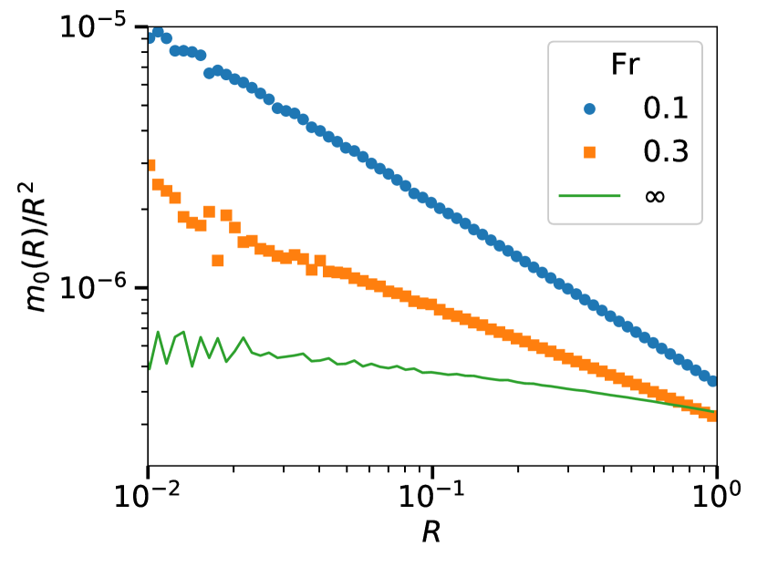
Figure 1: (color online) (a) $m_{0}(R)/R^{2}$ as a function of $R$ for $\mbox{St}=3.02$ and three different values of Fr. (b) Real space correlation dimension $d_{\rm 2}$ as a function of St for three different values of Fr.

Fig. (1)(a) shows plots of $m_{0}(R)/R^{2}$ as a function of $R$ for $\mbox{St}=3.02$ and three different values of Fr. We observe that $m_{0}(R)$ has a power-law dependence on $R$ with exponent equals to $d_{\rm 2}-1$. For $\mbox{Fr}=\infty$ data shows no clustering as $m_{0}(R)/R^{2}$ is independent of $R$. We observe that for the same St but $\mbox{Fr}=0.3$, and $0.1$ there is a significant amount of clustering. In Fig. (1)(b), we plot real space correlation dimension $d_{\rm 2}$ as a function of St for three different values of Fr. We find that for $\mbox{Fr}=0.1$ and $0.3$ and $\mbox{St}>1$, $d_{\rm 2}$ is small compared to $\mbox{Fr}=\infty$. This implies that the settling enhances the clustering for $\mbox{St}>1$ for the values of Fr considered here. This is consistent with the results of Refs. Bec et al. (2014). We also observe that for $\mbox{Fr}=0.1$ and $0.3$, $d_{\rm 2}$ becomes constant for large values of St. This indicates that the clustering does not depends on St for large values of St, this is consistent with the experimental observation of Refs Sumbekova et al. (2017); Petersen et al. (2019). For the range of St and Fr studied here, $d_{\rm 2}$ remains less than $d$, hence the phase space correlation dimension $D_{2}=d_{\rm 2}$.

III.2 Joint distribution of $R$ and $V_{R}$

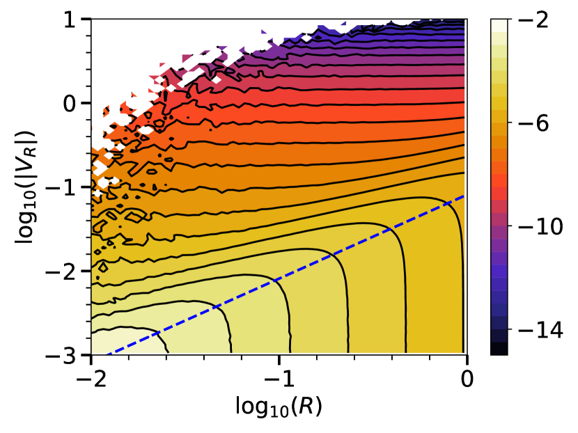
Figure 2: (color online) (a) Contour plots of $\log_{10}{(\mathcal{P}(R,V_{R})/R^{2})}$ for $\mbox{St}=2.11$ and $\mbox{Fr}=0.1$. (b) $\mathcal{P}(R,V_{R})/R^{2}$ for $R=0.1$, $\mbox{St}=2.11$, plotted for three different values of Fr. Solid lines in (b) have slopes equal to $D_{2}-4$.

Fig. (2) (a) shows the joint distribution $\mathcal{P}(R,|V_{R}|)/R^{2}$ for $\mbox{St}=2.11$ and $\mbox{Fr}=0.1$. The dashed blue line shows $|V_{R}|=z^{\ast}R$, where $z^{\ast}\simeq 0.1$ is found by fitting a line to the data. We find that the value of $z^{\ast}$ does not depends much on St, this is consistent with the results of  Bhatnagar et al. (2018b). We also observe that $z^{\ast}$ has a very week dependence on Fr but, we do not have many values of Fr to comment on this dependence. We observe that for $|V_{R}|<z^{\ast}R$, contour lines are vertical which implies that the distribution depends only on the separation $R$. For $|V_{R}|>z^{\ast}R$ contour lines are horizontal, implying that it depends only on $|V_{R}|$ in this regime. Similar nature of the distributions $\mathcal{P}(R,|V_{R}|)$ is observed for zero gravity ($\mbox{Fr}=\infty$) case in Refs. Bhatnagar et al. (2018a, b). In Fig. (2) (b), we plot the distribution $\mathcal{P}(R,V_{R})$ for $R=0.1$, $\mbox{St}=2.4$, and for three different values of Fr. We find that same as no-gravity case distributions have a power-law tail with scaling exponent $D_{2}-4$. As $D_{2}$ changes with Fr see Fig. (1), values of scaling exponents also changes. Observe that as we decrease Fr, power-law tails of the distributions become steeper. This implies that the mean and rms values of $|V_{R}|$ also decrease as gravity increases.

To understand collisions of particles one would like to know the distribution of $V_{R}$ at $R=2a$, where $a$ is the radius of the particle. For a given value of St, the radius depends on the density ratio $\rho_{\rm p}/\rho$ (as described at the beginning of Section III). For example, for $\mbox{St}=2.11$ and $\rho_{\rm p}/\rho=10^{3}$, value of $a/\eta$ is roughly $0.1$, hence data for $R<0.1$ in Fig. (2) (a) is irrelevant for this density ratio. For a different value of $\rho_{\rm p}/\rho$ and the same value of St, one would need the distribution at a different value of $R$, therefor covering a range of $R$ is useful to know the statistics of $V_{R}(R=2a)$ for a range of $\rho_{\rm p}/\rho$.

III.3 Effect of anisotropy

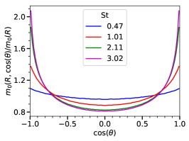
Figure 3: (color online) (a) $0$-th moment as a function of $\cos{(\theta)}$ for $R=0.5$ normalized by its average over $\cos{(\theta)}$ for $\mbox{Fr}=0.1$ and four different values of St. (b) $m^{\ell}_{0}$ for $\ell=0,2$ and $4$ plotted as a function of $R$ for $\mbox{St}=3.02$. (c) measure of anisotropy $m^{2}_{0}/m^{0}_{0}$ plotted as function of $R$ for $\mbox{Fr}=0.1$ and four different values of St.

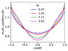
Figure 4: (color online) (a) $1$-th moment as a function of $\cos{(\theta)}$ for $R=0.5$ normalized by its average over $\cos{(\theta)}$ for $\mbox{Fr}=0.1$ and four different values of St. (b) $m^{\ell}_{1}$ for $\ell=0$ and $2$ plotted as a function of $R$ for $\mbox{St}=3.02$. (c) measure of anisotropy $m^{2}_{1}/m^{0}_{1}$ plotted as function of $R$ for $\mbox{Fr}=0.1$ and four different values of St.

Above calculations do not take in to account the anisotropy due to the presence of gravity. To compute the anisotropic contributions, we can obtain the joint distribution $\mathcal{P}(R,|V_{R}|,\cos(\theta))$, where $\theta$ is the angle between ${\bm{R}}$ and direction of gravity $\hat{z}$. We compute the moments $m_{\rm p}(R,\cos{(\theta)})$ of this distribution and use spherical harmonics decomposition. A function $f(R,\theta,\phi)$ that depends on spherical co-ordinates $R$, $\theta$, and $\phi$ can be expressed as a linear combination of Spherical harmonics $Y_{\ell}^{m}(\cos(\theta),\phi)$ as:

$$f(R,\theta,\phi)=\sum_{\ell=0}^{\infty}\sum_{m=-\ell}^{\ell}f_{\ell}^{m}(R)Y_{\ell}^{m}(\cos(\theta),\phi)$$ (6)

As there is no dependence on the azimuthal angle $\phi$ in our system, only $m=0$ modes are present. We can write:

$$m_{\rm p}(R,\cos(\theta))=\sum_{\ell}m_{\rm p}^{\ell}(R)P_{\ell}(\cos{(\theta)}),$$ (7)

here $P_{\ell}(x)$ is the Legendre polynomial of order $\ell$. As $m_{\rm p}(R,\cos(\theta))$ is a symmetric function of $\cos(\theta)$, all coefficients $m_{\rm p}^{\ell}(R)$ for odd values of $\ell$ vanish.

$m_{0}(R,\cos(\theta))$ is plotted in Fig. (3)(a) for $\mbox{Fr}=0.1$ and four different values of St, for $R=0.5$. $m^{0}_{0}(R)$, $m^{2}_{0}(R)$, and $m^{4}_{0}(R)$ are plotted in Fig. (3)(b) for $\mbox{St}=3.02$ and $\mbox{Fr}=0.1$. We find that $m^{\ell}_{0}(R)=C_{\ell}R^{\zeta_{\ell}}$. Exponents $\zeta_{\ell}$ are independent of $\ell$ and are equal to $d_{\rm 2}$ whereas the coefficients $C_{\ell}$ is zero for odd $\ell$ and decrease with $\ell$ for even $\ell$.

To measure the degree of anisotropy we plot $m^{2}_{0}/m^{0}_{0}$ as a function of $R$ for different values of St in Fig. (3)(c). We observe that this ratio does not depend on $R$ for the range of $R$ shown here. This is because both $m^{2}_{0}$ and $m^{0}_{0}$ scales with the same power as a function of $R$. We also find that anisotropy increases with increasing St.

In Fig. (4), we repeat this analysis for $m_{1}(R,\cos(\theta))$. Fig. (4) (b) shows plots for $m^{0}_{1}$ and $m^{2}_{1}$ as a function of $R$ for $\mbox{St}=3.03$ and $\mbox{Fr}=0.1$. Both of these coefficients show a power-law behaviour with roughly the same exponent. This is more clear from the plots of $m^{2}_{1}/m^{0}_{1}$ as a function of $R$ shown in Fig. (4) (c). It can be seen that the curves for higher values of St are not constant as a function of $R$, but dependence is very weak.

III.4 Mean collision velocity

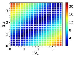
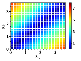
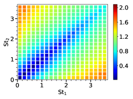
Figure 5: (color online) Mean $V_{\rm n}$ plotted as a function of $\mbox{St}_{\rm 1}$ and $\mbox{St}_{\rm 2}$, for $\mbox{Fr}=0.1$ (left), $\mbox{Fr}=0.3$ (middle), and $\mbox{Fr}=\infty$ (right).

The mean rate of collision depends on the relative velocity of particles when the separation between their centre of masses is equal to the sum of their radii. We define this as collision velocity $V_{\rm n}$ (see Eq. (5) and text before it). In Fig. (5) we plot the mean of $V_{\rm n}$ as a function of $\mbox{St}_{\rm 1}$ and $\mbox{St}_{\rm 2}$, for $\mbox{Fr}=0.3,0.1$, and $\infty$. We observe that the qualitative nature of these plot changes due to gravity. Along the diagonal $\mbox{St}_{\rm 1}=\mbox{St}_{\rm 2}$, values for non zero gravity are smaller compared to no gravity case. Away from diagonal for different sized particles mean of $V_{\rm n}$ becomes a function of $|\mbox{St}_{\rm 1}-\mbox{St}_{\rm 2}|$ for the settling particles. We also notice that values for settling particles away from the diagonal are much higher compared to particles with $\mbox{Fr}=\infty$.

To analyze it more quantitatively, we plot $\left\langle V_{\rm n}\right\rangle$ for $\mbox{St}_{\rm 1}=\mbox{St}_{\rm 2}=\mbox{St}$ in Fig. (6) (a), here $\left\langle\right\rangle$ denotes the mean. We observe that as Fr decrease $\left\langle V_{\rm n}\right\rangle$ decrease. In Fig. (6) (b) we plot $\left\langle V_{\rm n}\right\rangle$ as a function of $\mbox{St}_{\rm 2}$ for $\mbox{St}_{\rm 1}=0.1$. In this case, we find that $\left\langle V_{\rm n}\right\rangle$ increases significantly as Fr is decreased. Solid lines in this plot show the $\left\langle V_{\rm n}\right\rangle$ for particles settling under gravity in a fluid at rest.

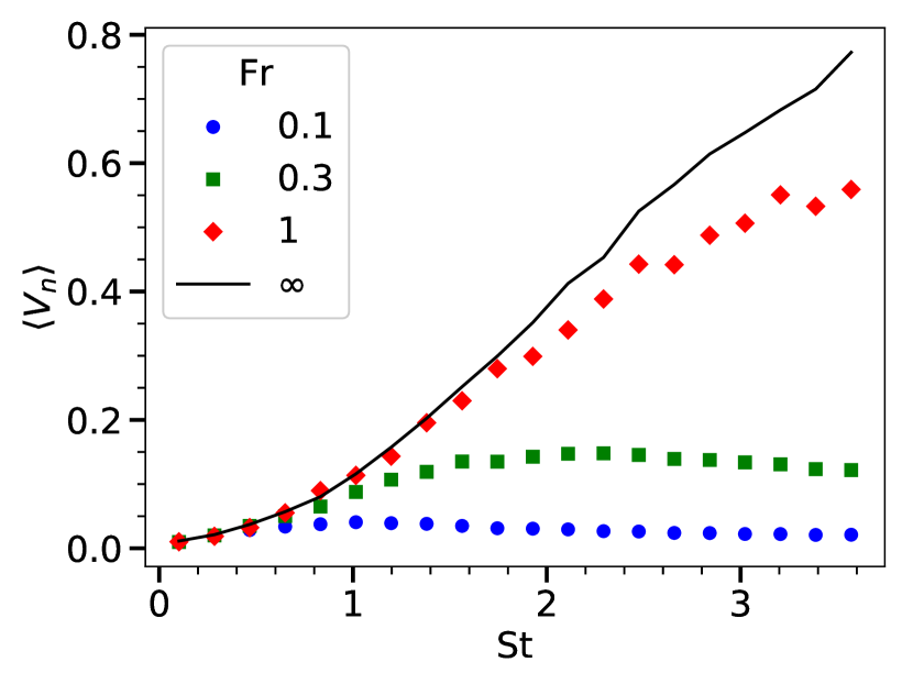
Figure 6: (color online) Mean of $V_{\rm n}$ at $R=a_{1}+a_{2}$ for $\mbox{St}_{\rm 1}=\mbox{St}_{\rm 2}$ (top) and for $\mbox{St}_{\rm 1}=0.1$ as a function of $\mbox{St}_{\rm 2}$ (bottom), for different values of Fr.

IV Conclusions

We have studied the effect of gravity on the relative velocities of particles suspended in turbulent flow by using direct numerical simulations. We explored a range of St and Fr that is relevant for small droplets in clouds. Our results show that joint PDFs of $R$ and $|V_{R}|$ has a form that is qualitatively similar to the one obtained without gravity. It is shown that for separations smaller than the Kolmogorov scale $\eta$ ($R<1$ in nondimensional units), there exist a scale $z^{\ast}$ such that joint PDF is independent of $|V_{R}|$ for $|V_{R}|<z^{\ast}R$, and is independent of $R$ for $|V_{R}|>z^{\ast}R$. We also show that PDFs of $|V_{R}|$ for a fixed value of $R$ scales as $|V_{R}|^{D_{2}-d-1}$ for some range of $|V_{R}|$. The phase space correlation dimension $D_{2}$ that measures the clustering of the particles in position-velocity phase-space is modified by the presence of gravity. For $\mbox{St}>1$, $D_{2}$ has a smaller value for $\mbox{Fr}=0.3$ and $0.1$ compared to $D_{2}$ for $\mbox{Fr}=\infty$. This implies that the position- and phase-space clustering is increased by the gravity for $\mbox{St}>1$.

We compute the moments of these joint PDFs of $R$ and $|V_{R}|$ as a function of $R$ and angle $\theta$ between the separation vector ${\bm{R}}$ and the direction of gravity. We showed that the moments depend on the $\cos{(\theta)}$ for a constant value of $R$. This indicates anisotropy in the system due to the presence of gravity. To characterize this anisotropy, we use a spherical harmonic decomposition and compute coefficients of order $\ell=0,2,$ and $4$. We found that all these coefficient have a power-law dependence on $R$. Exponents of the power-law is found to be the same for all values of $\ell$ that can be obtained for $0$-th and $1$-th order moments. We define the degree of anisotropy as the ratio of $\ell=2$ and $\ell=0$ coefficients. As both the coefficients scale with the same exponent, degree of anisotropy is independent of $R$, for $R<1$. A similar analysis of anisotropy is done in Ref. Ireland et al. (2016) for $R>1$. This study shows that for larger $R$, the degree of anisotropy depends on $R$ and goes to $0$ for very large values of $R$.

We define the velocity of collision $V_{\rm n}$ as the radial component of the relative velocity of two particles separated by the sum of their radii, when two particles are approaching each other. We calculated the mean of $V_{\rm n}$ as a function of $\mbox{St}_{\rm 1}$ and $\mbox{St}_{\rm 2}$ and found that it changes qualitatively from the zero-gravity case. Due to the presence of gravity mean of $V_{\rm n}$ becomes a function of $\mid\mbox{St}_{\rm 1}-\mbox{St}_{\rm 2}\mid$ alone. Furthermore, for particles with equal St, mean $V_{\rm n}$ decreases as Fr decreases, i.e., gravity increases. This decrease is more pronounced at higher St than at lower ones. For particle having different values of St the qualitative behaviour is opposite, the mean collision velocity increase as Fr decreases. For $\mbox{St}_{\rm 1}\neq\mbox{St}_{\rm 2}$ collision velocity is determined by the difference in the settling velocities of two particles.

Joint PDFs of $R$ and $|V_{R}|$ in the presence of gravity are studied for the first time in this paper. Refs. Parishani et al. (2015); Ireland et al. (2016) have studied the PDFs of $V_{R}$ for small values of $R$ but power-law nature of the PDFs is not shown. Real space correlation dimension $d_{\rm 2}$ for settling particles is studied in Ref. Bec et al. (2014). This study does not take into account the anisotropy due to the presence of gravity. Our study shows that the scaling exponents $d_{\rm 2}$ for anisotropic contributions are the same, but the amplitudes are different. Our results also show that gravity can have a significant effect on the collision velocities of particles having St between $0.5$ and $3$ and hence should be taken in to account in the studies relevant for cloud droplets in this range of St.

V Acknowledgments

We thank Dhrubaditya Mitra, K. Gustafsson, B. Mehlig, and J. Bec for useful discussions. This work is supported by the grant Bottlenecks for particle growth in turbulent aerosols from the Knut and Alice Wallenberg Foundation (Dnr. KAW 2014.0048), by Vetenskapsradet [grants 2013-3992 and 2017-03865], and Formas [grant number 2014-585]. Computational resources were provided by the Swedish National Infrastructure for Computing (SNIC) at PDC.

References

- Shaw (2003) R. A. Shaw, Annual Review of Fluid Mechanics 35, 183 (2003).
- Pruppacher and Klett (2010) H. Pruppacher and J. Klett, Microphysics of Clouds and Precipitation, Vol. 18 (Springer Science & Business Media, 2010).
- Grabowski and Wang (2013) W. W. Grabowski and L.-P. Wang, Annual Review of Fluid Mechanics 45, 293 (2013).
- Maxey and Riley (1983) M. R. Maxey and J. J. Riley, Physics of Fluids 26, 883 (1983).
- Daitche and Tél (2014) A. Daitche and T. Tél, New Journal of Physics 16, 073008 (2014).
- Daitche (2015) A. Daitche, Journal of Fluid Mechanics 782, 567 (2015).
- Vaillancourt and Yau (2000) P. A. Vaillancourt and M. Yau, Bulletin of the American Meteorological Society 81, 285 (2000).
- Ayala et al. (2008) O. Ayala, B. Rosa, L.-P. Wang, and W. W. Grabowski, New Journal of Physics 10, 075015 (2008).
- Rosa et al. (2016) B. Rosa, H. Parishani, O. Ayala, and L.-P. Wang, International Journal of Multiphase Flow 83, 217 (2016).
- Good et al. (2014) G. Good, P. Ireland, G. Bewley, E. Bodenschatz, L. Collins, and Z. Warhaft, Journal of Fluid Mechanics 759 (2014).
- Bec et al. (2007) J. Bec, L. Biferale, M. Cencini, A. Lanotte, S. Musacchio, and F. Toschi, Physical review letters 98, 084502 (2007).
- Falkovich and Pumir (2007) G. Falkovich and A. Pumir, Journal of the Atmospheric Sciences 64, 4497 (2007).
- Wilkinson and Mehlig (2005) M. Wilkinson and B. Mehlig, EPL (Europhysics Letters) 71, 186 (2005).
- Wilkinson et al. (2006) M. Wilkinson, B. Mehlig, and V. Bezuglyy, Physical review letters 97, 048501 (2006).
- Gustavsson and Mehlig (2011) K. Gustavsson and B. Mehlig, Physical Review E 84, 045304 (2011).
- Gustavsson and Mehlig (2014) K. Gustavsson and B. Mehlig, Journal of Turbulence 15, 34 (2014).
- Perrin and Jonker (2015) V. E. Perrin and H. J. Jonker, Physical Review E 92, 043022 (2015).
- Bhatnagar et al. (2018a) A. Bhatnagar, K. Gustavsson, and D. Mitra, Physical Review E 97, 023105 (2018a).
- James and Ray (2017) M. James and S. S. Ray, Scientific Reports 7, 12231 (2017).
- Maxey (1987) M. Maxey, Journal of Fluid Mechanics 174, 441 (1987).
- Wang and Maxey (1993) L.-P. Wang and M. R. Maxey, Journal of fluid mechanics 256, 27 (1993).
- Bec et al. (2014) J. Bec, H. Homann, and S. S. Ray, Physical review letters 112, 184501 (2014).
- Gustavsson et al. (2014) K. Gustavsson, S. Vajedi, and B. Mehlig, Physical Review Letters 112, 214501 (2014).
- Ireland et al. (2016) P. J. Ireland, A. D. Bragg, and L. R. Collins, Journal of Fluid Mechanics 796, 659 (2016).
- Sumbekova et al. (2017) S. Sumbekova, A. Cartellier, A. Aliseda, and M. Bourgoin, Physical Review Fluids 2, 024302 (2017).
- Petersen et al. (2019) A. J. Petersen, L. Baker, and F. Coletti, Journal of Fluid Mechanics 864, 925 (2019).
- Obligado et al. (2014) M. Obligado, T. Teitelbaum, A. Cartellier, P. Mininni, and M. Bourgoin, Journal of Turbulence 15, 293 (2014).
- Parishani et al. (2015) H. Parishani, O. Ayala, B. Rosa, L.-P. Wang, and W. Grabowski, Physics of Fluids 27, 033304 (2015).
- Onishi et al. (2009) R. Onishi, K. Takahashi, and S. Komori, Physics of Fluids 21, 125108 (2009).
- Woittiez et al. (2009) E. J. Woittiez, H. J. Jonker, and L. M. Portela, Journal of the atmospheric sciences 66, 1926 (2009).
- Dhariwal and Bragg (2018) R. Dhariwal and A. D. Bragg, Journal of Fluid Mechanics 839, 594 (2018).
- Brandenburg and Dobler (2002) A. Brandenburg and W. Dobler, Computer Physics Communications 147, 471 (2002).
- Bhatnagar et al. (2018b) A. Bhatnagar, K. Gustavsson, B. Mehlig, and D. Mitra, Physical Review E 98, 063107 (2018b).
- Williamson (1980) J. Williamson, Journal of Computational Physics 35, 48 (1980).
- Brandenburg (2001) A. Brandenburg, ApJ 550, 824 (2001).
- Higham (2001) D. Higham, SIAM Review 43, 525 (2001).
- Dobler et al. (2003) W. Dobler, N. E. L. Haugen, T. A. Yousef, and A. Brandenburg, Physical Review E 68, 026304 (2003).
- Haugen et al. (2003) N. E. L. Haugen, A. Brandenburg, and W. Dobler, The Astrophysical Journal Letters 597, L141 (2003).
- Haugen and Brandenburg (2004) N. E. L. Haugen and A. Brandenburg, Phys. Rev. E 70, 026405 (2004).
- Note (1) Radius of the particles is given by .