Revisiting oscillon formation in KKLT scenario

Abstract

KKLT scenario has succeeded in stabilizing the volume modulus and constructing metastable de Sitter (dS) vacua in type IIB string theory. We revisit to investigate the possibility of the oscillon (or I-ball) formation in the KKLT scenario when the volume modulus is initially displaced from the dS minimum. Special attention is paid to physically realistic initial conditions of the volume modulus, which was not taken in the literature. Using lattice simulations, we find that oscillons do not form unless the volume modulus is initially placed at very near the local maximum, which requires severe fine-tuning.

I Introduction

String theory, in general, contains numerous scalar fields, including the so-called moduli fields which determine the shape and size of extra dimensions. It was difficult for some time to achieve realistic phenomenological consequences from them since stabilization of the compactification of extra dimensions (i.e., moduli) remained to be an unsolved poser. Among them, it was most difficult to stabilize the volume modulus, also called the Kähler modulus. However, a possible solution to this problem was first proposed in Kachru et al. (2003), known as the KKLT scenario, eventually followed by the solution such as the Large Volume Scenario Balasubramanian et al. (2005). These scenarios succeeded not only in stabilizing the volume moduli in type IIB string theory, but also in enabling to construct metastable de Sitter (dS) vacua, opening the doors to explain observational cosmology by string theory.

It is believed that these moduli might change the course of the history of the standard cosmology in the early Universe by adding an extra matter (i.e., moduli) dominated era, which can lead to additional contributions of dark radiation Cicoli et al. (2013); Higaki and Takahashi (2012), baryogenesis Allahverdi et al. (2016) and non-thermal productions of dark matter Allahverdi et al. (2013). It is also natural to ask what the phenomenological consequences are when the volume moduli are displaced from the dS minimum in these scenarios. Thus, we focus on their cosmological dynamics in the KKLT scenario.

The phenomenon that we are particularly interested in is the production of oscillons Bogolyubsky and Makhankov (1976); Gleiser (1994); Copeland et al. (1995). Oscillons are spatially localized and long-lived non-topological solitons that could form when the scalar field $\phi$ oscillates around the minimum of a certain potential. For them to form, the potential needs to be slightly shallower than quadratic, at least in some regions of the field amplitude, and the perturbations of the scalar field must grow sufficiently as well. Oscillons are known to appear in various types of potentials, such as inflaton potentials Amin et al. (2012); McDonald (2002); Lozanov and Amin (2018); Hasegawa and Hong (2018), axion-like potentials Kolb and Tkachev (1994); Hong et al. (2018); Kawasaki et al. (2019), etc. It is also noteworthy that the stability of the oscillon is ensured by an adiabatic invariant $I$ Kasuya et al. (2003); Kawasaki et al. (2015), since it can be defined as the scalar configuration of the energy minimum with fixed $I$, which is why they are also called I-balls. When oscillons are generated, they can have a large impact on the cosmological evolution of the Universe: they could dominate the energy density of the universe and delay thermalization Gleiser (2007). In particular, it could be a source of characteristic gravitational waves Zhou et al. (2013); Antusch et al. (2018a), which may give some indications for string theories.

The oscillon formation in models based on string theory including the KKLT was examined before in Antusch et al. (2018b) to some extent. However, we find that the initial conditions of the volume modulus is not natural and appropriate in that paper. We therefore consider physically sensible initial values of the volume modulus and the Hubble parameter $H$, which would change the results of the simulations, and lead to different conclusions.

The paper is organized as follows. In Sec. II, we briefly review the potential of the volume modulus in the KKLT scenario. In Sec. III, we reexamine the growth of the instability using Floquet analysis following the procedures in Antusch et al. (2018b). In Sec. IV, we present the results of lattice simulations. The last section is devoted to conclusions. Throughout the paper we set the reduced Planck mass to $M_{P}=1$.

II KKLT model

In this section, we derive the potential of the volume modulus $T$ in the KKLT scenario, which is used in the lattice simulations of the oscillon formation. The relevant Kähler potential and superpotential in the simplest case are

$$K=-3\ln(T+\bar{T}),\quad W=W_{0}+Ae^{-\kappa T},$$ (1)

respectively, where $W_{0}$ is the superpotential after fluxes stabilize the axion–dilaton and complex structure moduli. The second term in the superpotential comes from gaugino condensation of $N$ D7-baranes with $\kappa=2\pi/N$, or wrapped Euclidean D3 brane instantons with $\kappa=2\pi$. In either case, $A$ is independent of the volume modulus and $\kappa\sim{\cal O}(1)$. Although the volume modulus is generically a complex scalar field ($T=\sigma+i\theta$), here we simply set the imaginary component $\theta$ to zero following Kachru et al. (2003). Then the potential can be obtained as

$$V(\sigma)=\frac{\kappa Ae^{-\kappa\sigma}}{2\sigma^{2}}\left[(1+\frac{\kappa}{3}\sigma)Ae^{-\kappa\sigma}+W_{0}\right].$$ (2)

This potential has the AdS vacuum, and must be lifted to a metastable dS vacuum by adding a small positive uplifting term as

$$\delta V=\frac{D}{\sigma^{3}},$$ (3)

which is achieved, for example, by the effects from anti-D3 branes where $D$ is a positive constant. The value of $D$ is fine-tuned so that the potential of the minimum is slightly positive, realizing the current stage of acceleration of the Universe. Another example of uplifting terms could arise using D7 branes Burgess et al. (2003). The exponent of $\sigma$ of the uplifting term depends on each mechanism. The total Lagrangian including the kinetic term is finally given by

$${\cal L}=\sqrt{-g}\left[\frac{3}{4\sigma^{2}}(\partial\sigma)^{2}-\left(V(\sigma)+\frac{D}{\sigma^{3}}\right)\right],$$ (4)

in the FLRW background

$$ds^{2}=dt^{2}-a^{2}(t)d{\bf x}^{2},$$ (5)

with $a(t)$ being the scale factor, and $g$ is the determinant of the metric $g_{\mu\nu}$.

Introducing a canonically normalized scalar field $\phi$ as

$$\phi=\frac{\sqrt{6}}{2}\ln(T+\bar{T})=\frac{\sqrt{6}}{2}\ln(2\sigma),$$ (6)

we obtain the Lagrangian as

$${\cal L}=\sqrt{-g}\left[\frac{1}{2}(\partial\phi)^{2}-V(\phi)\right],$$ (7)

where

$$V(\phi)=\frac{\kappa A\exp\left(-\kappa\frac{e^{\sqrt{6}\phi/3}}{2}\right)}{2(\frac{e^{\sqrt{6}\phi/3}}{2})^{2}}\left\{\left[1+\frac{\kappa}{3}\left(\frac{e^{\sqrt{6}\phi/3}}{2}\right)\right]A\exp\left(-\kappa\frac{e^{\sqrt{6}\phi/3}}{2}\right)+W_{0}\right\}+\frac{D}{\left(\frac{e^{\sqrt{6}\phi/3}}{2}\right)^{3}}.$$ (8)

In our numerical simulations, we adopt the following parameter ranges,

$$-10^{-5}\leq W_{0}\leq-10^{-12},\quad\quad 1\leq A\leq 10,\quad\quad 1\leq\kappa\leq 2\pi,$$ (9)

which are the same as used in Antusch et al. (2018b) by the same reasons explained there. Figure 1 shows an example of the KKLT potential.

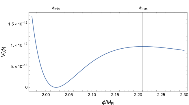
Figure 1: Potential of KKLT described by equation (8) in the case of $W_{0}=-10^{-5},A=10,\kappa=2\pi$ and $D=3.17\times 10^{-11}$. $\phi_{\text{min}}$ and $\phi_{\text{max}}$ are the field values at the minimum and the local maximum of the potential, respectively.

III Floquet Analysis

We first conduct the Floquet analysis in this section to discuss the growth of amplitudes of the perturbations, following Antusch et al. (2018b). This analysis can be applied when the fluctuations of the scalar field are small compared to the homogeneous and oscillating background field. Let us write the scalar field $\phi$ with the homogeneous background and the perturbation as

$$\phi(t,{\bf x})=\phi(t)+\delta\phi(t,{\bf x}).$$ (10)

The equation of motion of the homogeneous component is

$$\ddot{\phi}(t)+3H\dot{\phi}(t)+V^{\prime}(\phi(t))=0.$$ (11)

For the perturbation, we decompose it into Fourier modes $\delta\phi_{k}$:

$$\delta\phi(t,{\bf x})=\int\frac{d^{3}k}{(2\pi)^{3}}\delta\phi_{k}(t)e^{-i{\bf k}{\bf x}}.$$ (12)

The Fourier modes then obey the following equation:

$$\delta\ddot{\phi}_{k}+3H\delta\dot{\phi}_{k}+\left(\frac{k^{2}}{a^{2}(t)}+V^{\prime\prime}(\phi(t))\right)\delta\phi_{k}=0.$$ (13)

In the Floquet analysis, we ignore the expansion of the Universe and use the Minkowski space. Hence, equations (11) and (13) reduce respectively to

$$\ddot{\phi}(t)+V^{\prime}(\phi(t)) =0,$$ (14)

$$\delta\ddot{\phi}_{k}+\left[k^{2}+V^{\prime\prime}(\phi(t))\right]\delta\phi_{k} =0.$$ (15)

According to the Floquet theorem, the solution of equation (15) is given by

$$\delta\phi_{k}(t)=P_{+}(t)e^{\mu_{k}t}+P_{-}(t)e^{-\mu_{k}t},$$ (16)

where $\mu_{k}$ is the Floquet exponent and $P_{\pm}$ are periodic functions with the same period as the oscillation period of the background field, which we denote by $T$. Therefore, Re$(\mu_{k})\neq 0$ indicates instability growth of the fluctuation modes known as parametric resonanceShtanov et al. (1995); Kofman et al. (1996, 1997). The Floquet exponents can be obtained as follows. We solve the two equations (14) and (15) simultaneously from $t=0$ to $t=T$ for two sets of orthogonal initial conditions:

$$\delta\phi_{k,1}(0)=1,\ \delta\dot{\phi}_{k,1}(0)=0\quad{\rm and}\quad\delta\phi_{k,2}(0)=0,\ \delta\dot{\phi}_{k,2}(0)=1.$$ (17)

Floquet exponents are then computed by

$${\rm Re}(\mu_{k}^{\pm})=\frac{1}{T}\ln\left|\frac{1}{2}\left(\delta\phi_{k,1}+\delta\dot{\phi}_{k,2}\pm\sqrt{\left(\delta\phi_{k,1}-\delta\dot{\phi}_{k,2}\right)^{2}+4\delta\phi_{k,2}\delta\dot{\phi}_{k,1}}\right)\right|,$$ (18)

where all the quantities within the logarithm are evaluated at $t=T$ (see Amin et al. (2014) for more details). We compare the real part of the Floquet exponent to the mass of the modulus at the potential minimum,

$$m\equiv\left.\sqrt{\frac{\partial^{2}V(\phi)}{\partial\phi^{2}}}\right|_{\rm min},$$ (19)

since the timescale of the oscillation can be considered as $m^{-1}$ for most of the range of the initial field amplitude $\phi_{\rm initial}$.

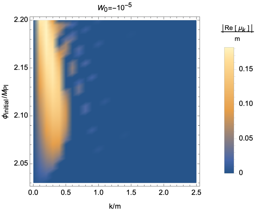
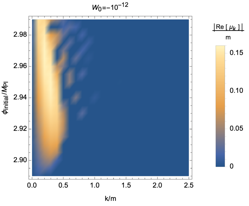
Figure 2: Floquet exponents of the KKLT model in units of the modulus mass for $W_{0}=-10^{-5},A=10,\kappa=2\pi$ (left) and $W_{0}=-10^{-12},A=10,\kappa=2\pi$ (right).

Figure 2 shows the results of the Floquet analysis for $W_{0}=-10^{-5},A=10,\kappa=2\pi$ (left) and $W_{0}=-10^{-12},A=10,\kappa=2\pi$ (right). In both cases, there exists a broad instability band at $k\lesssim 0.5m$, but the value of the exponent there is ${\rm Re}(\mu_{k})/m\sim 0.1$, which is generically not enough for the fluctuation modes to grow. Thus, it seems hard for the oscillon formation to take place.

However, the tachyonic instability could occur when the modulus field is initially placed near the local maximum of the potential, where the curvature of the potential (the second derivative of the potential $V^{\prime\prime}(\phi)$) is negative. Then the modes with wavenumbers with $k^{2}+V^{\prime\prime}(\phi)<0$ grow exponentially, which might result in the non-linear interactions among the fields leading to the formation of oscillons. We will see if this could happen in the lattice simulations in the next section.

IV Lattice Simulation

IV.1 Setups

We study the non-linear dynamics of the scalar field of the KKLT model by using a modified version of Lattice-Easy Felder and Tkachev (2008), solving the following equation on the lattices:

$$\ddot{\phi}+3\frac{\dot{a}}{a}\dot{\phi}-\frac{1}{a^{2}}\nabla^{2}\phi+\frac{\partial V(\phi)}{\partial\phi}=0.$$ (20)

The volume modulus starts to roll down the potential when the Hubble parameter becomes smaller than the curvature of the potential. We can thus naturally set the initial value of the homogeneous field, $\phi_{\rm init}$, and the Hubble parameter at that time, by

$$H_{\rm initial}=m_{\rm eff}(\phi_{\rm initial}),$$ (21)

where we define as

$$m_{\text{eff}}(\phi)\equiv\sqrt{\left|\frac{\partial^{2}V(\phi)}{\partial\phi^{2}}\right|},$$ (22)

together with the initial value of the time derivative of the field being $\dot{\phi}_{\text{initial}}=0$. Notice that this is the crucial difference from those adopted in Antusch et al. (2018b), in which they set

$$H_{\rm initial}=\sqrt{\frac{V(\phi_{\rm initial})}{3}}\quad{\rm for}\quad\phi_{\rm initial}=\phi_{\rm min}+\frac{\phi_{\rm max}-\phi_{\rm inf}}{2},\quad{\rm and}\quad\dot{\phi}_{\text{initial}}=0,$$ (23)

where $\phi_{\rm min}$, $\phi_{\rm max}$, and $\phi_{\rm inf}$ are the field values at the minimun, maximun, and the inflection point of the potential, respectively. Since $m_{\text{eff}}(\phi_{\rm intial})$ is larger than $\sqrt{V(\phi_{\text{initial}})/3}$ by about one order of magnitude for the majority of the field amplitudes, the field should have already rolled down if the latter had been adopted as the Hubble parameter. Therefore, the initial condition $\dot{\phi}_{\text{initial}}=0$ in Antusch et al. (2018b) is impossible to hold. As shown below, the naturally realized value of the Hubble parameter (21) forbids the generation of oscillons for an even wider range of $\phi_{\text{initial}}$.

As for the initial fluctuations of the scalar field, quantum vacuum fluctuations are used whose magnitude and phase follow the Rayleigh distribution and the random uniform distribution, respectively (see Felder and Tkachev (2008); Polarski and Starobinsky (1996); Khlebnikov and Tkachev (1996)). We assume the Universe is matter-dominated and evolve the scale factor accordingly starting from $a=1$.

We perform simulations using the rescaled variables

$$\phi_{pr}\equiv a\phi,\quad\vec{x}_{pr}\equiv m\vec{x},\quad dt_{pr}\equiv m\frac{dt}{a}$$ (24)

on the two-dimensional lattices, since we need high enough resolution with reasonable computation time. The scale factor evolves in the program as

$$a=\left(\frac{1}{2}m_{\rm eff}(\phi_{\rm initial})t_{pr}+1\right)^{2}.$$ (25)

We set the simulation parameters as described in Table 1, and adopt the model parameters with the ranges shown in (9) as mentioned.

Table 1: Parameters adopted in our simulations.

Box size	$L_{pr}=20$
Grid size	$N=1024^{2}$
Final time	$t_{f\_pr}=60$
Time-step	$dt_{pr}=5\times 10^{-3}$

IV.2 Results

We focus on showing the results of the case with $W_{0}=-10^{-5}$, $A=10$, and $\kappa=2\pi$, for two representative initial field values $\phi_{\rm initial}$. Figure 3 represents the evolution of the mean $\langle\phi\rangle$ and the variance $\sqrt{\langle\delta\phi^{2}\rangle}$ as a function of the scale factor for $\phi_{\text{initial}}=2.2$ (top) and $\phi_{\text{initial}}=2.2105$ (bottom), where $\phi_{\text{max}}=2.2105818...$. The solid black line indicates the field value at the inflection point of the potential.

We do not see that the fluctuations grow for most of the initial values of the field ($\phi_{\text{initial}}\lesssim 2.2$) as expected from the Floquet analysis, where the case for $\phi_{\text{initial}}=2.2$ is shown in the top panels of Fig. 3.

On the other hand, we see that the fluctuations grow by one order of magnitude at $a(t)\sim 6$ for $\phi_{\text{initial}}=2.2105$ shown in the bottom panels of Fig. 3. This is because, when the field starts at very near the local maximum, it stays in the negative-curvature region of the potential for a sufficiently long time, so that the Hubble parameter becomes small enough to cause the aforementioned tachyonic instability. In addition, the fluctuations slightly experience another boost from $a(t)\sim 15$ due to parametric resonance. The growth of the fluctuations itself eventually comes to a halt because parametric resonance soon becomes inefficient when the amplitude of the fluctuations becomes almost as large as that of the homogenous mode, and the non-linear interactions by mode-mode couplings would be important thereafter. Then the amplitude starts to decrease due to the expansion of the Universe.

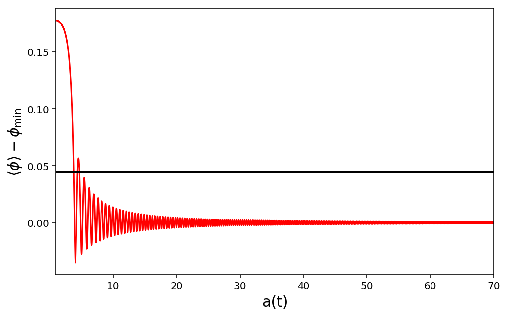
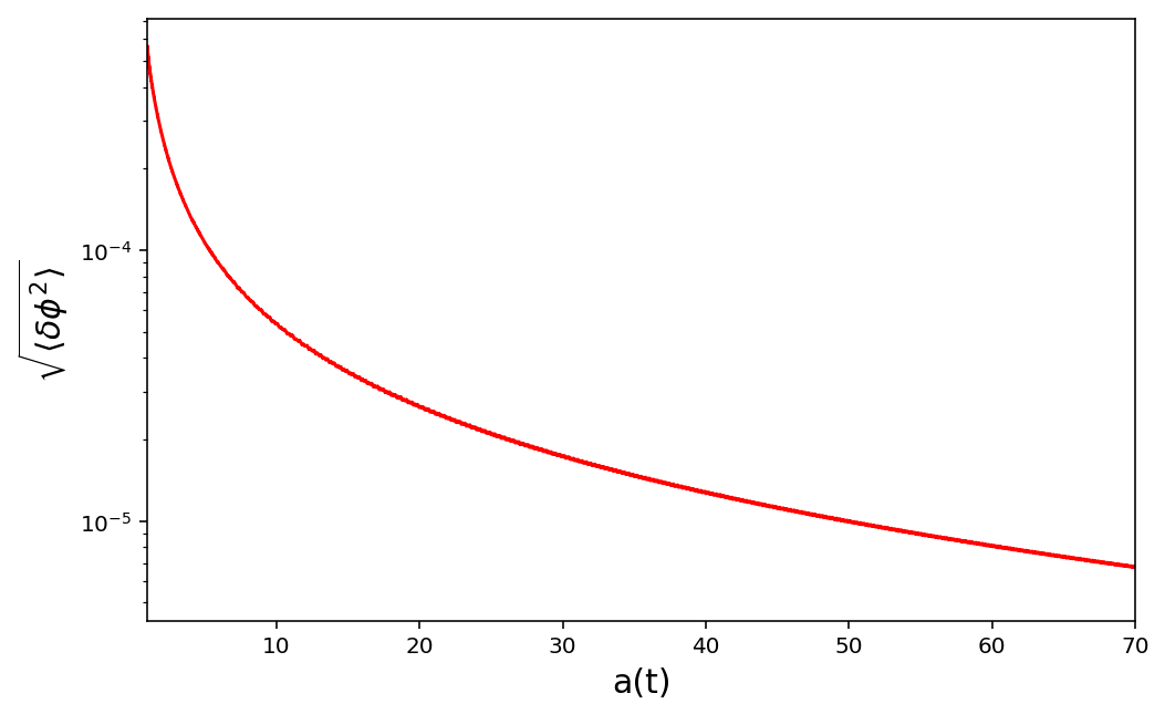
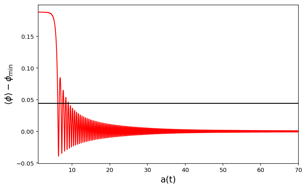
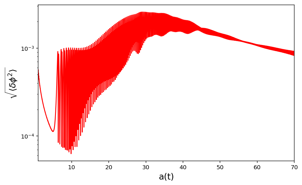
Figure 3: Evolution of the mean $\langle\phi\rangle$ (left) and the variance $\sqrt{\langle\delta\phi^{2}\rangle}$ (right) when $W_{0}=-10^{-5},A=10$, and $\kappa=2\pi$ as a function of the scale factor $a(t)$. The initial field values are taken to be $\phi_{\text{initial}}=2.2$ (top) and $\phi_{\text{initial}}=2.2105$ (bottom). The solid black line indicates the amplitude of the field at the inflection point of the potential.

Next, we show in Fig. 4 the spatial distribution of the energy density of the Kähler modulus,

$$\rho=\frac{1}{2}\dot{\phi}^{2}+\frac{1}{2a^{2}}|\nabla\phi|^{2}+V(\phi),$$ (26)

normalized by the average density $\langle\rho\rangle$ at $a=24.5$ (top left), $a=27.4$ (top right), $a=32.6$ (bottom left) and $a=44.2$ (bottom right) for $\phi_{\text{initial}}=2.2105$. As can be seen, localized regions of overdensity are produced. They dominate the system well after the growth of the fluctuations has stopped and seems to be so even after the end of the simulation $a\sim 70$. Since they could be a long-lived stable configuration, we can regard them as oscillons. We confirm the formation of oscillons for

$$2.2103\lesssim\phi_{\text{initial}}<\phi_{\text{max}},$$ (27)

which is a very narrow region near the local maximum of the potential.

We also perform numerical simulations for other values of the model parameters $W_{0},A$, and $\kappa$ within the range of (9), and obtain the same results that the oscillons can only form for a very narrow region of $\phi_{\text{initial}}$ near the local maximum of the potential. In addition, we check those cases having uplifting terms with different powers of $\sigma$, namely $D/\sigma,D/\sigma^{2}$, and $D/\sigma^{3}$, and find the same results with small quantitative but not qualitative differences. Therefore, we can safely say that severe fine-tuning for $\phi_{\text{initial}}$ is required for the oscillon formation in the KKLT model with the parameter range of (9).

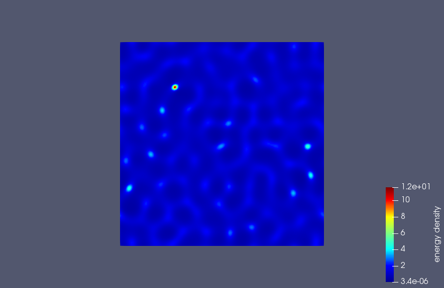
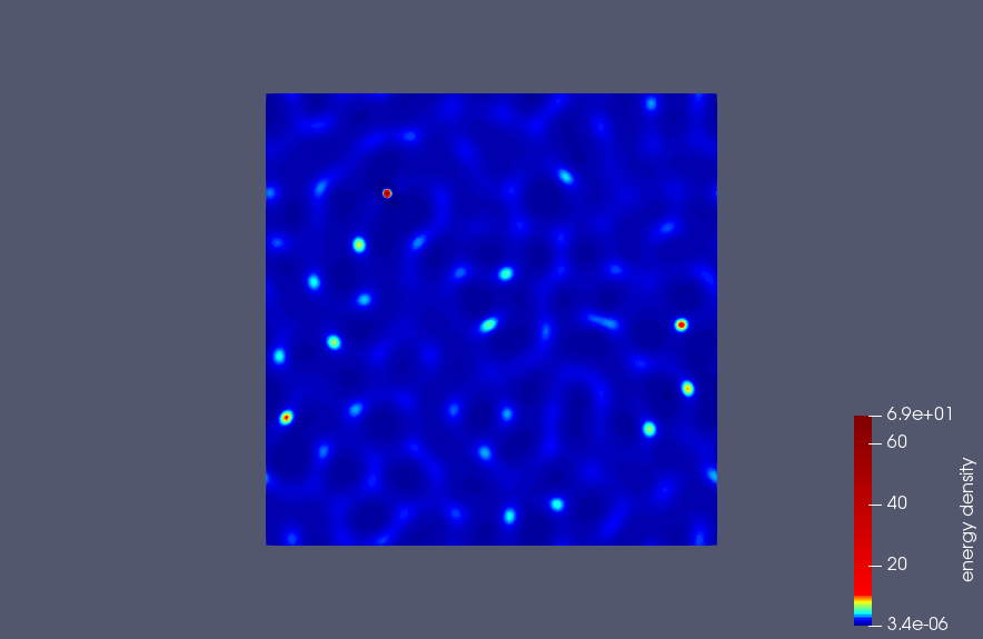
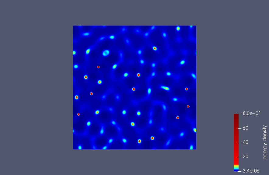
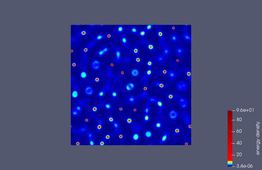
Figure 4: Energy density distribution $\rho/\langle\rho\rangle$ in the two dimensional lattice simulation for $W_{0}=-10^{-5}$, $A=10$, $\kappa=2\pi$ and $\phi_{\text{initial}}=2.2105$. The top left, top right, bottom left and bottom right panels correspond to the results at $a=24.5$, $a=27.4$, $a=32.6$ and $a=44.2$, respectively. The red regions indicate $\rho/\langle\rho\rangle\geq 10$.

V Conclusion and discussion

We have revisited to consider the possibility of the oscillon formation in KKLT model following the previous work of Antusch et al. (2018b). In there, they have concluded that the growth of the fluctuations is caused mostly by parametric resonance and that oscillons can be generated for $\phi_{\text{initial}}$ relatively close to the potential minimum. However, they set the initial value of the Hubble parameter as $H_{\text{initial}}=\sqrt{V(\phi_{\text{initial}})/3}$, which seems to be unnaturally small when the field begins to move towards the minimum of the potential.

In this paper, we have instead adopted the initial conditions as $H_{\text{initial}}=m_{\text{eff}}(\phi_{\rm initial})$, where $m_{\rm eff}$ is defined in (22), since it is this condition that the field starts rolling down the potential. This leads to the suppression of the growth of fluctuations, and the formation of oscillons is rather difficult.

By reconsidering the parameters thoroughly, we have thus come to a rather different conclusion: a large portion of the growth of the fluctuations, even if it does exist, is caused by tachyonic instability, and oscillons can only form if the volume modulus is initially placed at very near the local maximum, which requires severe fine-tuning.

References

- Kachru et al. (2003) S. Kachru, R. Kallosh, A. D. Linde, and S. P. Trivedi, Phys. Rev. D68, 046005 (2003), arXiv:hep-th/0301240 [hep-th] .
- Balasubramanian et al. (2005) V. Balasubramanian, P. Berglund, J. P. Conlon, and F. Quevedo, JHEP 03, 007 (2005), arXiv:hep-th/0502058 [hep-th] .
- Cicoli et al. (2013) M. Cicoli, J. P. Conlon, and F. Quevedo, Phys. Rev. D87, 043520 (2013), arXiv:1208.3562 [hep-ph] .
- Higaki and Takahashi (2012) T. Higaki and F. Takahashi, JHEP 11, 125 (2012), arXiv:1208.3563 [hep-ph] .
- Allahverdi et al. (2016) R. Allahverdi, M. Cicoli, and F. Muia, JHEP 06, 153 (2016), arXiv:1604.03120 [hep-th] .
- Allahverdi et al. (2013) R. Allahverdi, M. Cicoli, B. Dutta, and K. Sinha, Phys. Rev. D88, 095015 (2013), arXiv:1307.5086 [hep-ph] .
- Bogolyubsky and Makhankov (1976) I. L. Bogolyubsky and V. G. Makhankov, Pisma Zh. Eksp. Teor. Fiz. 24, 15 (1976).
- Gleiser (1994) M. Gleiser, Phys. Rev. D49, 2978 (1994), arXiv:hep-ph/9308279 [hep-ph] .
- Copeland et al. (1995) E. J. Copeland, M. Gleiser, and H. R. Muller, Phys. Rev. D52, 1920 (1995), arXiv:hep-ph/9503217 [hep-ph] .
- Amin et al. (2012) M. A. Amin, R. Easther, H. Finkel, R. Flauger, and M. P. Hertzberg, Phys. Rev. Lett. 108, 241302 (2012), arXiv:1106.3335 [astro-ph.CO] .
- McDonald (2002) J. McDonald, Phys. Rev. D66, 043525 (2002), arXiv:hep-ph/0105235 [hep-ph] .
- Lozanov and Amin (2018) K. D. Lozanov and M. A. Amin, Phys. Rev. D97, 023533 (2018), arXiv:1710.06851 [astro-ph.CO] .
- Hasegawa and Hong (2018) F. Hasegawa and J.-P. Hong, Phys. Rev. D97, 083514 (2018), arXiv:1710.07487 [astro-ph.CO] .
- Kolb and Tkachev (1994) E. W. Kolb and I. I. Tkachev, Phys. Rev. D49, 5040 (1994), arXiv:astro-ph/9311037 [astro-ph] .
- Hong et al. (2018) J.-P. Hong, M. Kawasaki, and M. Yamazaki, Phys. Rev. D98, 043531 (2018), arXiv:1711.10496 [astro-ph.CO] .
- Kawasaki et al. (2019) M. Kawasaki, W. Nakano, and E. Sonomoto, (2019), arXiv:1909.10805 [astro-ph.CO] .
- Kasuya et al. (2003) S. Kasuya, M. Kawasaki, and F. Takahashi, Phys. Lett. B559, 99 (2003), arXiv:hep-ph/0209358 [hep-ph] .
- Kawasaki et al. (2015) M. Kawasaki, F. Takahashi, and N. Takeda, Phys. Rev. D92, 105024 (2015), arXiv:1508.01028 [hep-th] .
- Gleiser (2007) M. Gleiser, Proceedings, 2nd International Workshop on Astronomy and Relativistic Astrophysics (IWARA 2005): Natal, Brazil, October 2-5, 2005, Int. J. Mod. Phys. D16, 219 (2007), arXiv:hep-th/0602187 [hep-th] .
- Zhou et al. (2013) S.-Y. Zhou, E. J. Copeland, R. Easther, H. Finkel, Z.-G. Mou, and P. M. Saffin, JHEP 10, 026 (2013), arXiv:1304.6094 [astro-ph.CO] .
- Antusch et al. (2018a) S. Antusch, F. Cefala, and S. Orani, JCAP 1803, 032 (2018a), arXiv:1712.03231 [astro-ph.CO] .
- Antusch et al. (2018b) S. Antusch, F. Cefala, S. Krippendorf, F. Muia, S. Orani, and F. Quevedo, JHEP 01, 083 (2018b), arXiv:1708.08922 [hep-th] .
- Burgess et al. (2003) C. P. Burgess, R. Kallosh, and F. Quevedo, JHEP 10, 056 (2003), arXiv:hep-th/0309187 [hep-th] .
- Shtanov et al. (1995) Y. Shtanov, J. H. Traschen, and R. H. Brandenberger, Phys. Rev. D51, 5438 (1995), arXiv:hep-ph/9407247 [hep-ph] .
- Kofman et al. (1996) L. Kofman, A. D. Linde, and A. A. Starobinsky, Phys. Rev. Lett. 76, 1011 (1996), arXiv:hep-th/9510119 [hep-th] .
- Kofman et al. (1997) L. Kofman, A. D. Linde, and A. A. Starobinsky, Phys. Rev. D56, 3258 (1997), arXiv:hep-ph/9704452 [hep-ph] .
- Amin et al. (2014) M. A. Amin, M. P. Hertzberg, D. I. Kaiser, and J. Karouby, Int. J. Mod. Phys. D24, 1530003 (2014), arXiv:1410.3808 [hep-ph] .
- Felder and Tkachev (2008) G. N. Felder and I. Tkachev, Comput. Phys. Commun. 178, 929 (2008), arXiv:hep-ph/0011159 [hep-ph] .
- Polarski and Starobinsky (1996) D. Polarski and A. A. Starobinsky, Class. Quant. Grav. 13, 377 (1996), arXiv:gr-qc/9504030 [gr-qc] .
- Khlebnikov and Tkachev (1996) S. Yu. Khlebnikov and I. I. Tkachev, Phys. Rev. Lett. 77, 219 (1996), arXiv:hep-ph/9603378 [hep-ph] .