The Simplex Tree: An Efficient Data Structure for General Simplicial Complexes

Abstract.

This paper introduces a new data structure, called simplex tree, to represent abstract simplicial complexes of any dimension. All faces of the simplicial complex are explicitly stored in a trie whose nodes are in bijection with the faces of the complex. This data structure allows to efficiently implement a large range of basic operations on simplicial complexes. We provide theoretical complexity analysis as well as detailed experimental results. We more specifically study Rips and witness complexes.

This article appeared in Algorithmica 2014 [9]. An extended abstract appeared in the proceedings of the European Symposium on Algorithms 2012 [8].

1. Introduction

Simplicial complexes are widely used in combinatorial and computational topology, and have found many applications in topological data analysis and geometric inference. A variety of simplicial complexes have been defined, for example the Čech complex, the Rips complex and the witness complex [13, 15]. However, the size of these structures grows very rapidly with the dimension of the data set, and their use in real applications has been quite limited so far.

We are aware of only a few works on the design of data structures for general simplicial complexes. Brisson [10] and Lienhardt [18] have introduced data structures to represent $d$-dimensional cell complexes, most notably subdivided manifolds. While those data structures have nice algebraic properties, they are very redundant and do not scale to large data sets or high dimensions. Zomorodian [24] has proposed the tidy set, a compact data structure to simplify a simplicial complex and compute its homology. Since the construction of the tidy set requires to compute the maximal faces of the simplicial complex, the method is especially designed for flag complexes. Flag complexes are a special type of simplicial complexes (to be defined later) whose combinatorial structure can be deduced from its graph. In particular, maximal faces of a flag complex can be computed without constructing explicitly the whole complex. In the same spirit, Attali et al. [3] have proposed the skeleton-blockers data structure. Again, the representation is general but it requires to compute blockers, the simplices which are not contained in the simplicial complex but whose proper subfaces are. Computing the blockers is difficult in general and details on the construction are given only for flag complexes, for which blockers can be easily obtained. As of now, there is no data structure for general simplicial complexes that scales to dimension and size. The best implementations have been restricted to flag complexes.

Our approach aims at combining both generality and scalability. We propose a tree representation for simplicial complexes. The nodes of the tree are in bijection with the simplices (of all dimensions) of the simplicial complex. In this way, our data structure, called a simplex tree, explicitly stores all the simplices of the complex but does not represent explicitly all the adjacency relations between the simplices, two simplices being adjacent if they share a common subface. Storing all the simplices provides generality, and the tree structure of our representation enables us to implement basic operations on simplicial complexes efficiently, in particular to retrieve incidence relations, ie to retrieve the faces that contain a given simplex or are contained in a given simplex.

The paper is organized as follows. In section 2.1, we describe the simplex tree and, in section 2.2, we detail the elementary operations on the simplex tree such as adjacency retrieval and maintainance of the data structure upon elementary modifications of the complex. In section 3, we describe and analyze the construction of flag complexes, witness complexes and relaxed witness complexes. An algorithm for inserting new vertices in the witness complex is also described. Finally, section 4 presents a thorough experimental analysis of the construction algorithms and compares our implementation with the softwares JPlex and Dionysus. Additional experiments are provided in appendix A.

1.1. Background

Simplicial complexes.

A simplicial complex is a pair $\mathcal{K}=(V,S)$ where $V$ is a finite set whose elements are called the vertices of $\mathcal{K}$ and $S$ is a set of non-empty subsets of $V$ that is required to satisfy the following two conditions :

1. $p\in V\Rightarrow\{p\}\in S$

2. $\sigma\in S,\tau\subseteq\sigma\Rightarrow\tau\in S$

Each element $\sigma\in S$ is called a simplex or a face of $\mathcal{K}$ and, if $\sigma\in S$ has precisely $s+1$ elements ($s\geq-1$), $\sigma$ is called an $s$-simplex and the dimension of $\sigma$ is $s$. The dimension of the simplicial complex $\mathcal{K}$ is the largest $k$ such that $S$ contains a $k$-simplex.

We define the $j$-skeleton, $j\geq 0$, of a simplicial complex $\mathcal{K}$ to be the simplicial complex made of the faces of $\mathcal{K}$ of dimension at most $j$. In particular, the $1$-skeleton of $\mathcal{K}$ contains the vertices and the edges of $\mathcal{K}$. The $1$-skeleton has the structure of a graph, and we will equivalently talk about the graph of the simplicial complex.

A subcomplex $\mathcal{K}^{\prime}=(V^{\prime},S^{\prime})$ of the simplicial complex $\mathcal{K}=(V,S)$ is a simplicial complex satisfying $V^{\prime}\subseteq V$ and $S^{\prime}\subseteq S$. In particular, the $j$-skeleton of a simplicial complex is a subcomplex.

Faces and cofaces.

A face of a simplex $\sigma=\{p_{0},\cdots,p_{s}\}$ is a simplex whose vertices form a subset of $\{p_{0},\cdots,p_{s}\}$. A proper face is a face different from $\sigma$ and the facets of $\sigma$ are its proper faces of maximal dimension. A simplex $\tau\in\mathcal{K}$ admitting $\sigma$ as a face is called a coface of $\sigma$. The subset of simplices consisting of all the cofaces of a simplex $\sigma\in\mathcal{K}$ is called the star of $\sigma$.

The link of a simplex $\sigma$ in a simplicial complex $\mathcal{K}=(V,S)$ is defined as the set of faces:

$${\rm Lk}(\sigma)=\{\tau\in S|\sigma\cup\tau\in S,\sigma\cap\tau=\emptyset\}$$

Filtration.

A filtration over a simplicial complex $\mathcal{K}$ is an ordering of the simplices of $\mathcal{K}$ such that all prefixes in the ordering are subcomplexes of $\mathcal{K}$. In particular, for two simplices $\tau$ and $\sigma$ in the simplicial complex such that $\tau\subsetneq\sigma$, $\tau$ appears before $\sigma$ in the ordering. Such an ordering may be given by a real number associated to the simplices of $\mathcal{K}$. The order of the simplices is simply the order of the real numbers.

2. Simplex Tree

In this section, we introduce a new data structure which can represent any simplicial complex. This data structure is a trie [5] which explicitly represents all the simplices and allows efficient implementation of basic operations on simplicial complexes.

2.1. Simplicial Complex and Trie

Let $\mathcal{K}=(V,S)$ be a simplicial complex of dimension $k$. The vertices are labeled from $1$ to $|V|$ and ordered accordingly.

We can thus associate to each simplex of $\mathcal{K}$ a word on the alphabet $1\cdots|V|$. Specifically, a $j$-simplex of $\mathcal{K}$ is uniquely represented as the word of length $j+1$ consisting of the ordered set of the labels of its $j+1$ vertices. Formally, let simplex $\sigma=\{v_{\ell_{0}},\cdots,v_{\ell_{j}}\}\in S$, where $v_{\ell_{i}}\in V$, $\ell_{i}\in\{1,\cdots,|V|\}$ and $\ell_{0}<\cdots<\ell_{j}$. $\sigma$ is then represented by the word $[\sigma]=[\ell_{0},\cdots,\ell_{j}]$. The last label of the word representation of a simplex $\sigma$ will be called the last label of $\sigma$ and denoted by $last(\sigma)$.

The simplicial complex $\mathcal{K}$ can be defined as a collection of words on an alphabet of size $|V|$. To compactly represent the set of simplices of $\mathcal{K}$, we store the corresponding words in a tree satisfying the following properties:

1. The nodes of the simplex tree are in bijection with the simplices (of all dimensions) of the complex. The root is associated to the empty face.

2. Each node of the tree, except the root, stores the label of a vertex. Specifically, a node associated to a simplex $\sigma\neq\emptyset$ stores the label $last(\sigma)$.

3. The vertices whose labels are encountered along a path from the root to a node associated to a simplex $\sigma$, are the vertices of $\sigma$. Along such a path, the labels are sorted by increasing order and each label appears no more than once.

We call this data structure the Simplex Tree of $\mathcal{K}$. It may be seen as a trie [5] on the words representing the simplices of the complex (Figure 1). The depth of the root is $0$ and the depth of a node is equal to the dimension of the simplex it represents plus one.

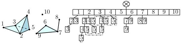
Figure 1. A simplicial complex on $10$ vertices and its simplex tree. The deepest node represents the tetrahedron of the complex. All the positions of a given label at a given depth are linked in a list, as illustrated in the case of label $5$.

In addition, we augment the data structure so as to quickly locate all the instances of a given label in the tree. Specifically, all the nodes at a same depth $j$ which contain a same label $\ell$ are linked in a circular list $L_{j}(\ell)$, as illustrated in Figure 1 for label $\ell=5$.

The children of the root of the simplex tree are called the top nodes. The top nodes are in bijection with the elements of $V$, the vertices of $\mathcal{K}$. Nodes which share the same parent (e.g. the top nodes) will be called sibling nodes.

We also attach to each set of sibling nodes a pointer to their parent so that we can access a parent in constant time.

We give a constructive definition of the simplex tree. Starting from an empty tree, we insert the words representing the simplices of the complex in the following manner. When inserting the word $[\sigma]=[\ell_{0},\cdots,\ell_{j}]$ we start from the root, and follow the path containing successively all labels $\ell_{0},\cdots,\ell_{i}$, where $[\ell_{0},\cdots,\ell_{i}]$ denotes the longest prefix of $[\sigma]$ already stored in the simplex tree. We then append to the node representing $[\ell_{0},\cdots,\ell_{i}]$ a path consisting of the nodes storing labels $\ell_{i+1},\cdots,\ell_{j}$.

It is easy to see that the three properties above are satisfied. Hence, if $\mathcal{K}$ consists of $|\mathcal{K}|$ simplices (including the empty face), the associated simplex tree contains exactly $|\mathcal{K}|$ nodes.

We use dictionaries with size linear in the number of elements they store (like a red-black tree or a hash table) for searching, inserting and removing elements among a set of sibling nodes. Consequently these additional structures do not change the asymptotic memory complexity of the simplex tree. For the top nodes, we simply use an array since the set of vertices $V$ is known and fixed. Let $\text{deg}(\mathcal{T})$ denote the maximal outdegree of a node, in the simplex tree $\mathcal{T}$, distinct from the root. Remark that $\text{deg}(\mathcal{T})$ is at most the maximal degree of a vertex in the graph of the simplicial complex. In the following, we will denote by $D_{\text{m}}$ the maximal number of operations needed to perform a search, an insertion or a removal in a dictionary of maximal size $\text{deg}(\mathcal{T})$ (for example, with red-black trees $D_{\text{m}}=O(\log(\text{deg}(\mathcal{T})))$ worst-case, with hash-tables $D_{\text{m}}=O(1)$ amortized). Some algorithms, that we describe later, require to intersect and to merge sets of sibling nodes. In order to compute fast set operations, we will prefer dictionaries which allow to traverse their elements in sorted order (e.g., red-black trees). We discuss the value of $D_{\text{m}}$ at the end of this section in the case where the points have a geometric structure.

We introduce two new notations for the analysis of the complexity of the algorithms. Given a simplex $\sigma\in\mathcal{K}$, we define $C_{\sigma}$ to be the number of cofaces of $\sigma$. Note that $C_{\sigma}$ only depends on the combinatorial structure of the simplicial complex $\mathcal{K}$. Let $\mathcal{T}$ be the simplex tree associated to $\mathcal{K}$. Given a label $\ell$ and an index $j$, we define $\mathcal{T}_{\ell}^{>j}$ to be the number of nodes of $\mathcal{T}$ at depth strictly greater than $j$ that store label $\ell$. These nodes represent the simplices of dimension at least $j$ that admit $\ell$ as their last label. $\mathcal{T}_{\ell}^{>j}$ depends on the labelling of the vertices and is bounded by $C_{\{v_{\ell}\}}$, the number of cofaces of the vertex with label $\ell$. For example, if $\ell$ is the greatest label, we have $\mathcal{T}_{\ell}^{>0}=C_{\{v_{\ell}\}}$, and if $\ell$ is the smallest label we have $\mathcal{T}_{\ell}^{>0}=1$ independently from the number of cofaces of $\{v_{\ell}\}$.

2.2. Operations on a Simplex Tree

We provide algorithms for:

• Search/Insert/Remove-simplex to search, insert or remove a single simplex, and Insert/Remove-full-simplex to insert a simplex and its subfaces or remove a simplex and its cofaces

• Locate-cofaces to locate the cofaces of a simplex

• Locate-facets to locate the facets of a simplex

• Elementary-collapse to proceed to an elementary collapse

• Edge-contraction to proceed to contract an edge

2.2.1. Insertions and Adjacency Retrieval

Insertions and Removals

Using the previous top-down traversal, we can search and insert a word of length $j$ in $O(jD_{\text{m}})$ operations.

We can extend this algorithm so as to insert a simplex and all its subfaces in the simplex tree. Let $\sigma$ be a simplex we want to insert with all its subfaces. Let $[\ell_{0},\cdots,\ell_{j}]$ be its word representation. For $i$ from $0$ to $j$ we insert, if not already present, a node $N_{\ell_{i}}$, storing label $\ell_{i}$, as a child of the root. We recursively call the algorithm on the subtree rooted at $N_{\ell_{i}}$ for the insertion of the suffix $[\ell_{i+1},\cdots,\ell_{j}]$. Since the number of subfaces of a simplex of dimension $j$ is $\sum_{i=0\cdots j+1}\binom{j+1}{i}=2^{j+1}$, this algorithm takes time $O(2^{j}D_{\text{m}})$.

We can also remove a simplex from the simplex tree. Note that to keep the property of being a simplicial complex, we need to remove all its cofaces as well. We locate them thanks to the algorithm described below.

Locate cofaces.

Computing the cofaces of a face is required to retrieve adjacency relations between faces. In particular, it is useful when traversing the complex or when removing a face. We also need to compute the cofaces of a face when contracting an edge (described later) or during the construction of the witness complex, described later in section 3.2.

If $\tau$ is represented by the word $[\ell_{0}\cdots\ell_{j}]$, the cofaces of $\tau$ are the simplices of $\mathcal{K}$ which are represented by words of the form $[\star\ell_{0}\star\ell_{1}\star\cdots\star\ell_{j}\star]$, where $\star$ represents an arbitrary word on the alphabet, possibly empty.

To locate all the words of the form $[\star\ell_{0}\star\ell_{1}\star\cdots\star\ell_{j}\star]$ in the simplex tree, we first find all the words of the form $[\star\ell_{0}\star\ell_{1}\star\cdots\star\ell_{j}]$. Using the lists $L_{i}(\ell_{j})$ ($i>j$), we find all the nodes at depth at least $j+1$ which contain label $\ell_{j}$. For each such node $N_{\ell_{j}}$, we traverse the tree upwards from $N_{\ell_{j}}$, looking for a word of the form $[\star\ell_{0}\star\ell_{1}\star\cdots\star\ell_{j}]$. If the search succeeds, the simplex represented by $N_{\ell_{j}}$ in the simplex tree is a coface of $\tau$, as well as all the simplices represented by the nodes in the subtree rooted at $N_{\ell_{j}}$, which have word representation of the form $[\star\ell_{0}\star\ell_{1}\star\cdots\star\ell_{j}\star]$. Remark that the cofaces of a simplex are represented by a set of subtrees in the simplex tree. The procedure searches only the roots of these subtrees.

The complexity for searching the cofaces of a simplex $\sigma$ of dimension $j$ depends on the number $\mathcal{T}_{last(\sigma)}^{>j}$ of nodes with label $last{(\sigma)}$ and depth at least $j+1$. If $k$ is the dimension of the simplicial complex, traversing the tree upwards takes $O(k)$ time. The complexity of this procedure is thus $O(k\mathcal{T}_{last(\sigma)}^{>j})$.

Locate Facets.

Locating the facets of a simplex efficiently is the key point of the incremental algorithm we use to construct witness complexes in section 3.2.

Given a simplex $\sigma$, we want to access the nodes of the simplex tree representing the facets of $\sigma$. If the word representation of $\sigma$ is $[\ell_{0},\cdots,\ell_{j}]$, the word representations of the facets of $\sigma$ are the words $[\ell_{0},\cdots,\widehat{\ell}_{i},\cdots,\ell_{j}]$, $0\leq i\leq j$, where $\widehat{\ell}_{i}$ indicates that $\ell_{i}$ is omitted. If we denote, as before, $N_{\ell_{i}},i=0,\cdots,j$ the nodes representing the words $[\ell_{0},\cdots,\ell_{i}],i=0,\cdots,j$ respectively, a traversal from the node representing $\sigma$ up to the root will exactly pass through the nodes $N_{\ell_{i}}$, $i=j,\cdots,0$. When reaching the node $N_{\ell_{i-1}}$, a search from $N_{\ell_{i-1}}$ downwards for the word $[\ell_{i+1},\cdots,\ell_{j}]$ locates (or proves the absence of) the facet $[\ell_{0},\cdots,\widehat{\ell}_{i},\cdots,\ell_{j}]$. See Figure 2 for a running example.

This procedure locates all the facets of the $j$-simplex $\sigma$ in $O(j^{2}D_{\text{m}})$ operations.

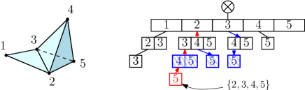
Figure 2. Facets location of the simplex $\sigma=\{2,3,4,5\}$, starting from the position of $\sigma$ in the simplex tree. The nodes representing the facets are colored in grey.

Experiments.

We report on the experimental performance of the facets and cofaces location algorithms. Figure 3 represents the average time for these operations on a simplex, as a function of the dimension of the simplex. We use the dataset Bro, consisting of points in $\mathbb{R}^{25}$, on top of which we build a relaxed witness complex with $300$ landmarks and $15,000$ witnesses, and relaxation parameter $\rho=0.15$. See section 4 for a detailed description of the experimental setup. We obtain a $13$-dimensional simplicial complex with $140,000$ faces in less than $3$ seconds.

Dim.Face	0	1	2	3	4	5	6	7	8	9	10	11	12	13
$\#$ Faces	300	2700	8057	15906	25271	30180	26568	17618	8900	3445	1015	217	30	2

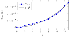
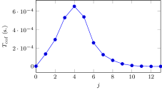
Figure 3. Repartition of the number of faces per dimension (top) and average time to compute the facets (left) and the cofaces (right) of a simplex of a given dimension.

The theoretical complexity for computing the facets of a $j$-simplex $\sigma$ is $O(j^{2}D_{\text{m}})$. As reported in Figure 3, the average time to search all facets of a $j$-simplex is well approximated by a quadratic function of the dimension $j$ (the standard error in the approximation is $2.0\%$).

A bound on the complexity of computing the cofaces of a $j$-simplex $\sigma$ is $O(k\mathcal{T}_{last(\sigma)}^{>j})$, where $\mathcal{T}_{last(\sigma)}^{>j}$ stands for the number of nodes in the simplex tree that store the label $last{(\sigma)}$ and have depth larger than $j+1$. Figure 3 provides experimental results for a random labelling of the vertices. As can be seen, the time for computing the cofaces of a simplex $\sigma$ is low, on average, when the dimension of $\sigma$ is either small ($0$ to $2$) or big ($6$ to $13$), and higher for intermediate dimensions ($3$ to $5$). The value $\mathcal{T}_{last(\sigma)}^{>j}$ in the complexity analysis depends on both the labelling of the vertices and the number of cofaces of the vertex $v_{last{(\sigma)}}$: these dependencies make the analysis of the algorithm quite difficult, and we let as an open problem to fully understand the experimental behavior of the algorithm as observed in Figure 3 (right).

2.2.2. Topology preserving operations

We show how to implement two topology preserving operations on a simplicial complex represented as a simplex tree. Such simplifications are, in particular, important in topological data analysis.

Elementary collapse.

We say that a simplex $\sigma$ is collapsible through one of its faces $\tau$ if $\sigma$ is the only coface of $\tau$, which can be checked by computing the cofaces of $\tau$. Such a pair $(\tau,\sigma)$ is called a free pair. Removing both faces of a free pair is an elementary collapse.

Since $\tau$ has no coface other than $\sigma$, either the node representing $\tau$ in the simplex tree is a leaf (and so is the node representing $\sigma$), or it has the node representing $\sigma$ as its unique child. An elementary collapse of the free pair $(\tau,\sigma)$ consists either in the removal of the two leaves representing $\tau$ and $\sigma$, or the removal of the subtree containing exactly two nodes: the node representing $\tau$ and the node representing $\sigma$.

Edge contraction.

Edge contractions are used in [3] as a tool for homotopy preserving simplification and in [14] for computing the persistent topology of data points. Let $\mathcal{K}$ be a simplicial complex and let $\{v_{\ell_{a}},v_{\ell_{b}}\}$ be an edge of $\mathcal{K}$ we want to contract. We say that we contract $v_{\ell_{b}}$ to $v_{\ell_{a}}$ meaning that $v_{\ell_{b}}$ is removed from the complex and the link of $v_{\ell_{a}}$ is augmented with the link of $v_{\ell_{b}}$. Formally, we define the map $f$ on the set of vertices $V$ which maps $v_{\ell_{b}}$ to $v_{\ell_{a}}$ and acts as the identity function for all other inputs:

$$f(u)=\left\{\begin{array}[]{ll}v_{\ell_{a}}&\qquad\mathrm{if}\quad u=v_{\ell_{b}}\\ u&\qquad\mathrm{otherwise}\\ \end{array}\right.$$

We then extend $f$ to all simplices $\sigma=\{v_{\ell_{0}},\cdots,v_{\ell_{j}}\}$ of $\mathcal{K}$ with $f(\sigma)=\{f(v_{\ell_{0}}),\cdots,f(v_{\ell_{j}})\}$. The contraction of $v_{\ell_{b}}$ to $v_{\ell_{a}}$ is defined as the operation which replaces $\mathcal{K}=(V,S)$ by $\mathcal{K}^{\prime}=(V\setminus\{v_{\ell_{b}}\},\{f(\sigma)|\sigma\in S)\}$. $\mathcal{K}^{\prime}$ is a simplicial complex.

It has been proved in [3] that contracting an edge $\{v_{\ell_{a}},v_{\ell_{b}}\}$ preserves the homotopy type of a simplicial complex whenever the link condition is satisfied:

$${\rm Lk}(\{v_{\ell_{a}},v_{\ell_{b}}\})={\rm Lk}(\{v_{\ell_{a}}\})\cap{\rm Lk}(\{v_{\ell_{b}}\})$$

This link condition can be checked using the Locate-cofaces algorithm described above.

Let $\sigma$ be a simplex of $\mathcal{K}$. We distinguish three cases : 1. $\sigma$ does not contain $v_{\ell_{b}}$ and remains unchanged; 2. $\sigma$ contains both $v_{\ell_{a}}$ and $v_{\ell_{b}}$, and $f(\sigma)=\sigma\setminus\{v_{\ell_{b}}\}$; $|f(\sigma)|=|\sigma|-1$ and $f(\sigma)$ is a strict subface of $\sigma$; 3. $\sigma$ contains $v_{\ell_{b}}$ but not $v_{\ell_{a}}$ and $f(\sigma)=\left(\sigma\setminus\{v_{\ell_{b}}\}\right)\cup\{v_{\ell_{a}}\}$, ($|f(\sigma)|=|\sigma|$).

Figure 4. Contraction of vertex $3$ to vertex $1$ and the associated modifications of the simplicial complex and of the simplex tree. The nodes which are removed are marked with a red cross, the subtrees which are moved are colored in blue.

We describe now how to compute the contraction of $v_{\ell_{b}}$ to $v_{\ell_{a}}$ when $\mathcal{K}$ is represented as a simplex tree. We suppose that the edge $\{v_{\ell_{a}},v_{\ell_{b}}\}$ is in the complex and, without loss of generality, $\ell_{a}<\ell_{b}$. All the simplices which do not contain $v_{\ell_{b}}$ remain unchanged and we do not consider them. If a simplex $\sigma$ contains both $v_{\ell_{a}}$ and $v_{\ell_{b}}$, it will become $\sigma\setminus\{v_{\ell_{b}}\}$, after edge contraction, which is a simplex already in $\mathcal{K}$. We simply remove $\sigma$ from the simplex tree. Finally, if $\sigma$ contains $v_{\ell_{b}}$ but not $v_{\ell_{a}}$, we need to remove $\sigma$ from the simplex tree and add the new simplex $\left(\sigma\setminus\{v_{\ell_{b}}\}\right)\cup\{v_{\ell_{a}}\}$.

We consider each node $N_{\ell_{b}}$ with label $\ell_{b}$ in turn. To do so, we use the lists $L_{j}(\ell)$ which link all nodes cointaining the label $\ell$ at depth $j$. Let $\sigma$ be the simplex represented by $N_{\ell_{b}}$. The algorithm traverses the tree upwards from $N_{\ell_{b}}$ and collects the vertices of $\sigma$. Let $T_{N_{\ell_{b}}}$ be the subtree rooted at $N_{\ell_{b}}$. As $\ell_{a}<\ell_{b}$, if $\sigma$ contains both $v_{\ell_{a}}$ and $v_{\ell_{b}}$, this will be true for all the simplices whose representative nodes are in $T_{N_{\ell_{b}}}$, and, if $\sigma$ contains only $v_{\ell_{b}}$, the same will be true for all the simplices whose representative nodes are in $T_{N_{\ell_{b}}}$. Consequently, if $\sigma$ contains both $v_{\ell_{a}}$ and $v_{\ell_{b}}$, we remove the whole subtree $T_{N_{\ell_{b}}}$ from the simplex tree. Otherwise, $\sigma$ contains only $v_{\ell_{b}}$, all words represented in $T_{N_{\ell_{b}}}$ are of the form $[\sigma^{\prime}]\centerdot[\sigma^{\prime\prime}]\centerdot[\ell_{b}]\centerdot[\sigma^{\prime\prime\prime}]$ and will be turned into words $[\sigma^{\prime}]\centerdot[\ell_{a}]\centerdot[\sigma^{\prime\prime}]\centerdot[\sigma^{\prime\prime\prime}]$ after edge contraction. We then have to move the subtree $T_{N_{\ell_{b}}}$ (except its root) from position $[\sigma^{\prime}]\centerdot[\sigma^{\prime\prime}]$ to position $[\sigma^{\prime}]\centerdot[\ell_{a}]\centerdot[\sigma^{\prime\prime}]$ in the simplex tree. If a subtree is already rooted at this position, we have to merge $T_{N_{\ell_{b}}}$ with this subtree as illustrated in Figure 4. In order to merge the subtree $T_{N_{\ell_{b}}}$ with the subtree rooted at the node representing the word $[\sigma^{\prime}]\centerdot[\ell_{a}]\centerdot[\sigma^{\prime\prime}]$, we can successively insert every node of $T_{N_{\ell_{b}}}$ in the corresponding set of sibling nodes, stored in a dictionary. See Figure 4.

We analyze the complexity of contracting an edge $\{v_{\ell_{a}},v_{\ell_{b}}\}$. For each node storing the label $\ell_{b}$, we traverse the tree upwards. This takes $O(k)$ time if the simplicial complex has dimension $k$. As there are $\mathcal{T}_{\ell_{b}}^{>0}$ such nodes, the total cost is $O(k\mathcal{T}_{\ell_{b}}^{>0})$. We also manipulate the subtrees rooted at the nodes storing label $\ell_{b}$. Specifically, either we remove such a subtree or we move a subtree by changing its parent node. In the latter case, we have to merge two subtrees. This is the more costly operation which takes, in the worst case, $O(D_{\text{m}})$ operations per node in the subtrees to be merged. As any node in such a subtree represents a coface of vertex $v_{\ell_{b}}$, the total number of nodes in all the subtrees we have to manipulate is at most $C_{\{v_{\ell_{b}}\}}$, and the manipulation of the subtrees takes $O(C_{\{v_{\ell_{b}}\}}D_{\text{m}})$ time. Consequently, the time needed to contract the edge $\{v_{\ell_{a}},v_{\ell_{b}}\}$ is $O(k\mathcal{T}_{\ell_{b}}^{>0}+C_{\{v_{\ell_{b}}\}}D_{\text{m}})$.

Remark on the value of $D_{\text{m}}$

: $D_{\text{m}}$ appears as a key value in the complexity analysis of the algorithms. Recall that $D_{\text{m}}$ is the maximal number of operations needed to perform a search, an insertion or a removal in a dictionary of maximal size $\text{deg}(\mathcal{T})$ in the simplex tree. We suppose in the following that the dictionaries used are red-black trees, in which case $D_{\text{m}}=O(\log(\text{deg}(\mathcal{T})))$. As mentioned earlier, $\text{deg}(\mathcal{T})$ is bounded by the maximal degree of a vertex in the graph of the simplicial complex. In the worst-case, if $n$ denotes the number of vertices of the simplicial complex, we have $\text{deg}(\mathcal{T})=O(n)$, and $D_{\text{m}}=O(\log(n))$. However, this bound can be improved in the case of simplicial complexes constructed on sparse data points sampled from a low dimensional manifold, an important case in practical applications. Let $\mathbb{M}$ be a $d$-manifold with bounded curvature, embedded in $\mathbb{R}^{D}$ and assume that the length of the longest (resp., shortest) edge of the simplicial complex has length at most $r$ (resp., at least $\epsilon$). Then, a volume argument shows that the maximal degree of a vertex in the simplicial complex is $\Theta((r/\epsilon)^{d})$. Hence, when $r=O(\epsilon)$, which is a typical situation when $S$ is an $\epsilon$-net of $\mathbb{M}$, the value of $D_{\text{m}}$ is $O(d)$ with a constant depending only on local geometric quantities.

3. Construction of Simplicial Complexes

In this section, we detail how to construct two important types of simplicial complexes, the flag and the witness complexes, using simplex trees.

3.1. Flag complexes

A flag complex is a simplicial complex whose combinatorial structure is entirely determined by its $1$-skeleton. Specifically, a simplex is in the flag complex if and only if its vertices form a clique in the graph of the simplicial complex, or, in other terms, if and only if its vertices are pairwise linked by an edge.

Expansion.

Given the $1$-skeleton of a flag complex, we call expansion of order $k$ the operation which reconstructs the $k$-skeleton of the flag complex. If the $1$-skeleton is stored in a simplex tree, the expansion of order $k$ consists in successively inserting all the simplices of the $k$-skeleton into the simplex tree.

Let $G=(V,E)$ be the graph of the simplicial complex, where $V$ is the set of vertices and $E\subseteq V\times V$ is the set of edges. For a vertex $v_{\ell}\in V$, we denote by

$$\mathcal{N}^{+}(v_{\ell})=\{\ell^{\prime}\in\{1,\cdots,|V|\}\mbox{ }|\mbox{ }(v_{\ell},v_{\ell^{\prime}})\in E\wedge\ell^{\prime}>\ell\}$$

the set of labels of the neighbors of $v_{\ell}$ in $G$ that are bigger than $\ell$. Let $N_{\ell_{j}}$ be the node in the tree that stores the label $\ell_{j}$ and represents the word $[\ell_{0},\cdots,\ell_{j}]$. The children of $N_{\ell_{j}}$ store the labels in $\mathcal{N}^{+}(v_{\ell_{0}})\cap\cdots\cap\mathcal{N}^{+}(v_{\ell_{j}})$. Indeed, the children of $N_{\ell_{j}}$ are neighbors in $G$ of the vertices $v_{\ell_{i}}$, $0\leq i\leq j$, (by definition of a clique) and must have a bigger label than $\ell_{0},\cdots,\ell_{j}$ (by construction of the simplex tree).

Consequently, the sibling nodes of $N_{\ell_{j}}$ are exactly the nodes that store the labels in $A=\mathcal{N}^{+}(v_{\ell_{0}})~{}\cap~{}\cdots~{}\cap~{}\mathcal{N}^{+}(v_{\ell_{j-1}})$, and the children of $N_{\ell_{j}}$ are exactly the nodes that store the labels in $A\cap\mathcal{N}^{+}(v_{\ell_{j}})$. See Figure 5.

For every vertex $v_{\ell}$, we have an easy access to $\mathcal{N}^{+}(v_{\ell})$ since $\mathcal{N}^{+}(v_{\ell})$ is exactly the set of labels stored in the children of the top node storing label $\ell$. We easily deduce an in-depth expansion algorithm.

The time complexity for the expansion algorithm depends on our ability to fastly compute intersections of the type $A\cap\mathcal{N}^{+}(v_{\ell_{j}})$. In all of our experiments on the Rips complex (defined below) we have observed that the time taken by the expansion algorithm depends linearly on the size of the output simplicial complex, for a fixed dimension. More details can be found in section 4 and appendix A.

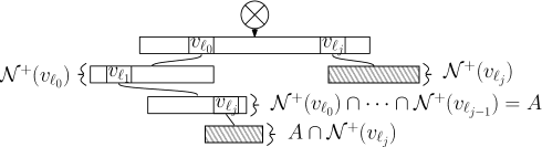
Figure 5. Representation of a set of sibling nodes as intersection of neighborhoods.

Rips Complex.

Rips complexes are geometric flag complexes which are popular in computational topology due to their simple construction and their good approximation properties [4, 12]. Given a set of vertices $V$ in a metric space and a parameter $r>0$, the Rips graph is defined as the graph whose set of vertices is $V$ and two vertices are joined by an edge if their distance is at most $r$. The Rips complex is the flag complex defined on top of this graph. We will use this complex for our experiments on the construction of flag complexes.

3.2. Witness complexes

The Witness Complex.

has been first introduced in [13]. Its definition involves two given sets of points in a metric space, the set of landmarks $L$ and the set of witnesses $W$.

Definition 3.1.

A witness $w\in W$ witnesses a simplex $\sigma\subseteq L$ iff:

$$\forall x\in\sigma\mbox{ and }\forall y\in L\setminus\sigma\mbox{ we have }\text{d}(w,x)\leq\text{d}(w,y)$$

For simplicity of exposition, we will suppose that no landmarks are at the exact same distance to a witness. In this case, a witness $w\in W$ witnesses a simplex $\sigma\subseteq L$ iff the vertices of $\sigma$ are the $|\sigma|$ nearest neighbors of $w$ in $L$. We study later the construction of the relaxed witness complex, which is a generalization of the witness complex which includes the case where points are not in general position.

The witness complex ${\rm Wit}(W,L)$ is the maximal simplicial complex, with vertices in $L$, whose faces admit a witness in $W$. Equivalently, a simplex belongs to the witness complex if and only if it is witnessed and all its facets belong to the witness complex. A simplex satisfying this property will be called fully witnessed.

Construction Algorithm.

We suppose the sets $L$ and $W$ to be finite and give them labels $\{1,\cdots,|L|\}$ and $\{1,\cdots,|W|\}$ respectively. We describe how to construct the $k$-skeleton of the witness complex, where $k$ may be any integer in $\{1,\cdots,|L|-1\}$.

Our construction algorithm is incremental, from lower to higher dimensions. At step $j$ we insert in the simplex tree the $j$-dimensional fully witnessed simplices.

During the construction of the $k$-skeleton of the witness complex, we need to access the nearest neighbors of the witnesses, in $L$. To do so, we compute the $k+1$ nearest neighbors of all the witnesses in a preprocessing phase, and store them in a $|W|\times(k+1)$ matrix. Given an index $j\in\{0,\cdots,k\}$ and a witness $w\in W$, we can then access in constant time the $(j+1)^{\text{th}}$ nearest neighbor of $w$. We denote this landmark by $s_{j}^{w}$. We maintain a list of active witnesses, initialized with $W$. We insert the vertices of ${\rm Wit}(W,L)$ in the simplex tree. For each witness $w\in W$ we insert a top node storing the label of the nearest neighbor of $w$ in $L$, if no such node already exists. $w$ is initially an active witness and we make it point to the node mentionned above, representing the $0$-dimensional simplex $w$ witnesses.

We maintain the following loop invariants:

1. at the beginning of iteration $j$, the simplex tree contains the $(j-1)$-skeleton of the witness complex ${\rm Wit}(W,L)$

2. the active witnesses are the elements of $W$ that witness a $(j-1)$-simplex of the complex; each active witness $w$ points to the node representing the $(j-1)$-simplex in the tree it witnesses.

At iteration $j\geq 1$, we traverse the list of active witnesses. Let $w$ be an active witness. We first retrieve the $(j+1)^{\text{th}}$ nearest neighbor $s_{j}^{w}$ of $w$ from the nearest neighbors matrix (Step 1). Let $\sigma_{j}$ be the $j$-simplex witnessed by $w$ and let us decompose the word representing $\sigma_{j}$ into $[\sigma_{j}]=[\sigma^{\prime}]\centerdot[s_{j}^{w}]\centerdot[\sigma^{\prime\prime}]$ (“$\centerdot$” denotes the concatenation of words). We then look for the location in the tree where $\sigma_{j}$ might be inserted (Step 2). To do so, we start at the node $N_{w}$ which represents the $(j-1)$-simplex witnessed by $w$. Observe that the word associated to the path from the root to $N_{w}$ is exactly $[\sigma^{\prime}]\centerdot[\sigma^{\prime\prime}]$. We walk $|[\sigma^{\prime\prime}]|$ steps up from $N_{w}$, reach the node representing $[\sigma^{\prime}]$ and then search downwards for the word $[s_{w}^{j}]\centerdot[\sigma^{\prime\prime}]$ (see Figure 6, left). The cost of this operation is $O(jD_{\text{m}})$.

If the node representing $\sigma_{j}$ exists, $\sigma_{j}$ has already been inserted; we update the pointer of $w$ and return. If the simplex tree contains neither this node nor its father, $\sigma_{j}$ is not fully witnessed because the facet represented by its longest prefix is missing. We consequently remove $w$ from the set of active witnesses. Lastly, if the node is not in the tree but its father is, we check whether $\sigma_{j}$ is fully witnessed. To do so, we search for the $j+1$ facets of $\sigma_{j}$ in the simplex tree (Step 3). The cost of this operation is $O(j^{2}D_{\text{m}})$ using the Locate-facets algorithm described in section 2.2. If $\sigma_{j}$ is fully witnessed, we insert $\sigma_{j}$ in the simplex tree and update the pointer of the active witness $w$. Else, we remove $w$ from the list of active witnesses (see Figure 6, right).

It is easily seen that the loop invariants are satisfied at the end of iteration $j$.

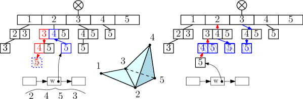
Figure 6. Third iteration of the witness complex construction. The active witness $w$ witnesses the tetrahedron $\{2,3,4,5\}$ and points to the triangle $\{2,4,5\}$. (Left) Search for the potential position of the simplex $\{2,3,4,5\}$ in the simplex tree. (Right) Facets location for simplex $\{2,3,4,5\}$, and update of the pointer of the active witness $w$.

Complexity.

The cost of accessing a neighbor of a witness using the nearest neighbors matrix is $O(1)$. We access a neighbor (Step 1) and locate a node in the simplex tree (Step 2) at most $k|W|$ times. In total, the cost of Steps 1 and 2 together is $O(|W|k^{2}D_{\text{m}})$. In Step 3, either we insert a new node in the simplex tree, which happens exactly $|\mathcal{K}|$ times (the number of faces in the complex), or we remove an active witness, which happens at most $|W|$ times. The total cost of Step 3 is thus $O((|\mathcal{K}|+|W|)k^{2}D_{\text{m}})$. In conclusion, constructing the $k$-skeleton of the witness complex takes time

$$O((|\mathcal{K}|+|W|)k^{2}D_{\text{m}}+k|W|)=O((|\mathcal{K}|+|W|)k^{2}D_{\text{m}}).$$

Landmark Insertion.

We present an algorithm to update the simplex tree under landmark insertions. Adding new vertices in witness complexes is used in [7] for manifold reconstruction. Given the set of landmarks $L$, the set of witnesses $W$ and the $k$-skeleton of the witness complex ${\rm Wit}(W,L)$ represented as a simplex tree, we take a new landmark point $x$ and we update the simplex tree so as to construct the simplex tree associated to ${\rm Wit}(W,L\cup\{x\})$. We assign to $x$ the biggest label $|L|+1$. We suppose to have at our disposal an oracle that can compute the subset $W^{x}\subseteq W$ of the witnesses that admit $x$ as one of their $k+1$ nearest neighbors. Computing $W^{x}$ is known as the reverse nearest neighbor search problem, which has been intensively studied in the past few years [2]. Let $w$ be a witness in $W^{x}$ and suppose $x$ is its $(i+1)^{\text{th}}$ nearest neighbor in $L\cup\{x\}$, with $0\leq i\leq k$. Let $\sigma_{j}\subseteq L$ be the $j$-dimensional simplex witnessed by $w$ in $L$ and let $\widetilde{\sigma_{j}}\subseteq L\cup\{x\}$ be the $j$-dimensional simplex witnessed by $w$ in $L\cup\{x\}$. Consequently, $\sigma_{j}=\widetilde{\sigma_{j}}$ for $j<i$ and $\sigma_{j}\neq\widetilde{\sigma_{j}}$ for $j\geq i$. We equip each node $N$ of the simplex tree with a counter of witnesses which maintains the number of witnesses that witness the simplex represented by $N$. As for the witness complex construction, we consider all nodes representing simplices witnessed by elements of $W^{x}$, proceeding by increasing dimensions. For a witness $w\in W^{x}$ and a dimension $j\geq i$, we decrement the witness counter of $\sigma_{j}$ and insert $\widetilde{\sigma_{j}}$ if and only if its facets are in the simplex tree. We remark that $[\widetilde{\sigma_{j}}]=[\sigma_{j-1}]\centerdot[x]$ because $x$ has the biggest label of all landmarks. We can thus access in time $O(D_{\text{m}})$ the position of the word $[\widetilde{\sigma_{j}}]$ since we have accessed the node representing $[\sigma_{j-1}]$ in the previous iteration of the algorithm.

If the witness counter of a node is turned down to $0$, the simplex $\sigma$ it represents is not witnessed anymore, and is consequently not part of ${\rm Wit}(W,L\cup\{x\})$. We remove the nodes representing $\sigma$ and its cofaces from the simplex tree, using Locate-cofaces.

Complexity.

The update procedure is a “local” variant of the witness complex construction, where, by “local”, we mean that we reconstruct only the star of vertex $x$. Let $C_{x}$ denote the number of cofaces of $x$ in ${\rm Wit}(W,L\cup\{x\})$ (or equivalently the size of its star). The same analysis as above shows that updating the simplicial complex takes time $O((|W^{x}|+C_{x})k^{2}D_{\text{m}})$, plus one call to the oracle to compute $W^{x}$.

Relaxed Witness Complex.

Given a relaxation parameter $\rho\geq 0$ we define the relaxed witness complex [13]:

Definition 3.2.

A witness $w\in W$ $\rho$-witnesses a simplex $\sigma\subseteq L$ iff:

$$\forall x\in\sigma\mbox{ and }\forall y\in L\setminus\sigma\mbox{ we have }d(w,x)\leq d(w,y)+\rho$$

The relaxed witness complex $\mbox{{\rm Wit}}^{\rho}$$(W,L)$ with parameter $\rho$ is the maximal simplicial complex, with vertices in $L$, whose faces admit a $\rho$-witness in $W$. For $\rho=0$, the relaxed witness complex is the standard witness complex. The parameter $\rho$ defines a filtration on the witness complex, which has been used in topological data analysis.

We resort to the same incremental algorithm as above. At each step $j$, we insert, for each witness $w$, the $j$-dimensional simplices which are $\rho$-witnessed by $w$. Differently from the standard witness complex, there may be more than one $j$-simplex that is witnessed by a given witness $w\in W$. Consequently, we do not maintain a pointer from each active witness to the last inserted simplex it witnesses. We use simple top-down insertions from the root of the simplex tree.

Given a witness $w$ and a dimension $j$, we generate all the $j$-dimensional simplices which are $\rho$-witnessed by $w$. For the ease of exposition, we suppose we are given the sorted list of nearest neighbors of $w$ in $L$, noted $\{z_{0}\cdots z_{|L|-1}\}$, and their distance to $w$, noted $m_{i}=\text{d}(w,z_{i})$, with $m_{0}\leq\cdots\leq m_{|L|-1}$, breaking ties arbitrarily. Note that if one wants to construct only the $k$-skeleton of the complex, it is sufficient to know the list of neighbors of $w$ that are at distance at most $m_{k}+\rho$ from $w$. We preprocess this list of neighbors for all witnesses. For $i\in\{0,\cdots,|L|-1\}$, we define the set $A_{i}$ of landmarks $z$ such that $m_{i}\leq d(w,z)\leq m_{i}+\rho$. For $i\leq j+1$, $w$ $\rho$-witnesses all the $j$-simplices that contain $\{z_{0},\cdots,z_{i-1}\}$ and a $(j+1-i)$-subset of $A_{i}$, provided $|A_{i}|\geq j+1-i$. We see that all $j$-simplices that are $\rho$-witnessed by $w$ are obtained this way, and exactly once, when $i$ ranges from $0$ to $j+1$.

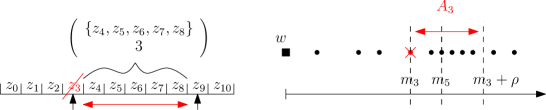
Figure 7. Computation of the $\rho$-witnessed simplices $\sigma$ of dimension $5$. If $z_{3}$ is the first neighbor of $w$ not in $\sigma$, then $\sigma$ contains $\{z_{0},z_{1},z_{2}\}$ and any $3$-uplet of $A_{3}=\{z_{4},\cdots,z_{8}\}$.

For all $i\in\{0,\cdots,j+1\}$, we compute $A_{i}$ and generate all the simplices which contain $\{z_{0},\cdots,z_{i-1}\}$ and a subset of $A_{i}$ of size $(j+1-i)$. In order to easily update $A_{i}$ when $i$ is incremented, we maintain two pointers to the list of neighbors, one to $z_{i}$ and the other to the end of $A_{i}$. We check in constant time if $A_{i}$ contains more than $j+1-i$ vertices, and compute all the subsets of $A_{i}$ of cardinality $j+1-i$ accordingly. See Figure 7.

Complexity.

Let $R_{j}$ be the number of $j$-simplices $\rho$-witnessed by $w$. Generating all those simplices takes $O(j+R_{j})$ time. Indeed, for all $i$ from $0$ to $j+1$, we construct $A_{i}$ and check whether $A_{i}$ contains more than $j+1-i$ elements. This is done by a simple traversal of the list of neighbors of $w$, which takes $O(j)$ time. Then, when $A_{i}$ contains more than $j+1-i$ elements, we generate all subsets of $A_{i}$ of size $j+1-i$ in time $O(\binom{|A_{i}|}{j+1-i})$. As each such subset leads to a $\rho$-witnessed simplex, the total cost for generating all those simplices is $O(R_{j})$.

We can deduce the complexity of the construction of the relaxed witness complex. Let $\mathcal{R}=\displaystyle\sum_{w\in W}\sum_{j=0\cdots k}R_{j}$ be the number of $\rho$-witnessed simplices we try to insert. The construction of the relaxed witness complex takes $O(\mathcal{R}k^{2}D_{\text{m}})$ operations. This bound is quite pessimistic and, in practice, we observed that the construction time is sensitive to the size of the output complex. Observe that the quantity analogous to $\mathcal{R}$ in the case of the standard witness complex was $k|W|$ and that the complexity was better due to our use of the notion of active witnesses.

4. Experiments

Data	$|\mathcal{P}|$	$D$	$d$	$r$	$T_{\mbox{g}}$	$|E|$	$T_{\mbox{Rips}}$	$|\mathcal{K}|$	$T_{\mbox{tot}}$	$T_{\mbox{tot}}/|\mathcal{K}|$
Bud	49,990	3	2	0.11	1.5	1,275,930	104.5	354,695,000	104.6	$3.0\cdot 10^{-7}$
Bro	15,000	25	?	0.019	0.6	3083	36.5	116,743,000	37.1	$3.2\cdot 10^{-7}$
Cy8	6,040	24	2	0.4	0.11	76,657	4.5	13,379,500	4.61	$3.4\cdot 10^{-7}$
Kl	90,000	5	2	0.075	0.46	1,120,000	68.1	233,557,000	68.5	$2.9\cdot 10^{-7}$
S4	50,000	5	4	0.28	2.2	1,422,490	95.1	275,126,000	97.3	$3.6\cdot 10^{-7}$

Data	$|L|$	$|W|$	$D$	$d$	$\rho$		$T_{\mbox{nn}}$	$T_{\mbox{$\mbox{{\rm Wit}}^{\rho}$}}$	$|\mathcal{K}|$	$T_{\mbox{tot}}$	$T_{\mbox{tot}}/|\mathcal{K}|$
Bud	10,000	49,990	3	2	0.12		1.	729.6	125,669,000	730.6	$0.58\cdot 10^{-5}$
Bro	3,000	15,000	25	?	0.01		9.9	107.6	2,589,860	117.5	$4.5\cdot 10^{-5}$
Cy8	800	6,040	24	2	0.23		0.38	161	997,344	161.2	$16\cdot 10^{-5}$
Kl	10,000	90,000	5	2	0.11		2.2	572	109,094,000	574.2	$0.53\cdot 10^{-5}$
S4	50,000	200,000	5	4	0.06		25.1	296.7	163,455,000	321.8	$0.20\cdot 10^{-5}$

Figure 8. Data, timings (in s.) and statistics for the construction of Rips complexes (TOP) and relaxed witness complexes (BOTTOM). All complexes are constructed up to embedding dimension.

In this section, we report on the performance of our algorithms on both real and synthetic data, and compare them to existing software. More specifically, we benchmark the construction of Rips complexes, witness complexes and relaxed witness complexes. Our implementations are in C++. We use the ANN library [21] to compute the $1$-skeleton graph of the Rips complex, and to compute the lists of nearest neighbors of the witnesses for the witness complexes. All timings are measured on a Linux machine with $3.00$ GHz processor and $32$ GB RAM. For its efficiency and flexibility, we use the map container of the Standard Template Library [23] for storing sets of sibling nodes, except for the top nodes which are stored in an array.

We use a variety of both real and synthetic datasets. Bud is a set of points sampled from the surface of the Stanford Buddha [1] in $\mathbb{R}^{3}$. Bro is a set of $5\times 5$ high-contrast patches derived from natural images, interpreted as vectors in $\mathbb{R}^{25}$, from the Brown database (with parameter $k=300$ and cut $30\%$) [11, 17]. Cy8 is a set of points in $\mathbb{R}^{24}$, sampled from the space of conformations of the cyclo-octane molecule [19], which is the union of two intersecting surfaces. Kl is a set of points sampled from the surface of the figure eight Klein Bottle embedded in $\mathbb{R}^{5}$. Finally S4 is a set of points uniformly distributed on the unit $4$-sphere in $\mathbb{R}^{5}$. Datasets are listed in Figure 8 with details on the sets of points $\mathcal{P}$ or landmarks $L$ and witnesses $W$, their size $|\mathcal{P}|$, $|L|$ and $|W|$, the ambient dimension $D$, the intrinsic dimension $d$ of the object the sample points belong to (if known), the parameter $r$ or $\rho$, the dimension $k$ up to which we construct the complexes, the time $T_{\mbox{g}}$ to construct the Rips graph or the time $T_{\mbox{nn}}$ to compute the lists of nearest neighbors of the witnesses, the number of edges $|E|$, the time for the construction of the Rips complex $T_{\mbox{Rips}}$ or for the construction of the witness complex $T_{\mbox{$\mbox{{\rm Wit}}^{\rho}$}}$, the size of the complex $|\mathcal{K}|$, and the total construction time $T_{\mbox{tot}}$ and average construction time per face $T_{\mbox{tot}}/|\mathcal{K}|$.

We test our algorithms on these datasets, and compare their performance with two existing softwares that are state-of-the-art. We compare our implementation to the JPlex [22] library and the Dionysus [20] library. The first is a Java package which can be used with Matlab and provides an implementation of the construction of Rips complexes and witness complexes. The second is implemented in C++ and provides an implementation of the construction of Rips complexes. Both libraries are widely used to construct simplicial complexes and to compute their persistent homology. We also provide an experimental analysis of the memory performance of our data structure compared to other representations. Unless mentioned otherwise, all simplicial complexes are computed up to the embedding dimension.

All timings are averaged over $10$ independent runs. Timings are provided by the clock function from the Standard C Library, and zero means that the measured time is below the resolution of the clock function. Experiments are stopped after one hour of computation, and data missing on plots means that the computation ran above this time limit.

For readability, we do not report on the performance of each algorithm on each dataset in this section, but the results presented are a faithful sample of what we have observed on other datasets. A complete set of experiments is reported in appendix A.

As illustrated in Figure 8, we are able to construct and represent both Rips and relaxed witness complexes of up to several hundred million faces in high dimensions, on all datasets.

Data structure in JPlex and Dionysus:

Both JPlex and Dionysus represent the combinatorial structure of a simplicial complex by its Hasse diagram. The Hasse diagram of a simplicial complex $\mathcal{K}$ is the graph whose nodes are in bijection with the simplices (of all dimensions) of the simplicial complex and where an edge links two nodes representing two simplices $\tau$ and $\sigma$ iff $\tau\subseteq\sigma$ and $\text{dim}(\sigma)=\text{dim}(\tau)+1$.

JPlex and Dionysus are libraries dedicated to topological data analysis, where only the construction of simplicial complexes and the computation of the facets of a simplex are necessary.

For a simplicial complex $\mathcal{K}$ of dimension $k$ and a simplex $\sigma\in\mathcal{K}$ of dimension $j$, the Hasse diagram has size $\Theta(k|\mathcal{K}|)$ and allows to compute Locate-facets$(\sigma)$ in time $O(j)$, whereas the simplex tree has size $\Theta(|\mathcal{K}|)$ and allows to compute Locate-facets$(\sigma)$ in time $O(j^{2}D_{\text{m}})$.

4.1. Memory Performance of the Simplex Tree

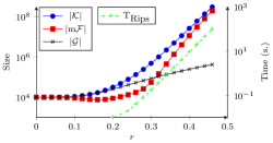
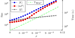
Figure 9. Statistics and timings for the Rips complex (Left) and the relaxed witness complex (Right) on S4.

In order to represent the combinatorial structure of an arbitrary simplicial complex, one needs to mark all maximal faces. Indeed, except in some special cases (like in flag complexes where all faces are determined by the $1$-skeleton of the complex), one cannot infer the existence of a simplex in a simplicial complex $\mathcal{K}$ from the existence of its faces in $\mathcal{K}$. Moreover, the number of maximal simplices of a $k$-dimensional simplicial complex is at least $|V|/(k+1)$. In the case, considered in this paper, where the vertices are identified by their labels, a minimal representation of the maximal simplices would then require at least $\Omega(\log|V|)$ bits per maximal face, for fixed $k$. The simplex tree uses $O(\log|V|)$ memory bits per face of any dimension. The following experiment compares the memory performance of the simplex tree with the minimal representation described above, and with the representation of the $1$-skeleton.

Figure 9 shows results for both Rips and relaxed witness complexes associated to $10,000$ points from S4 and various values of, respectively, the distance threshold $r$ and the relaxation parameter $\rho$. The figure plots the total number of faces $|\mathcal{K}|$, the number of maximal faces $|\mbox{m}\mathcal{F}|$, the size of the $1$-skeleton $|\mathcal{G}|$ and the construction times $T_{\mbox{Rips}}$ and $T_{\mbox{$\mbox{{\rm Wit}}^{\rho}$}}$.

As expected, the $1$-skeleton is significantly smaller than the two other representations. However, as explained earlier, a representation of the graph of the simplicial complex is only well suited for flag complexes.

As shown on the figure, the total number of faces and the number of maximal faces remain close along the experiment. Interestingly, we catch the topology of S4 when $r\approx 0.4$ for the Rips complex and $\rho\approx 0.08$ for the relaxed witness complex. For these “good” values of the parameters, the total number of faces is not much bigger than the number of maximal faces. Specifically, the total number of faces of the Rips complex is less than $2.3$ times bigger than the number of maximal faces, and the ratio is less than $2$ for the relaxed witness complex.

4.2. Construction of Rips Complexes

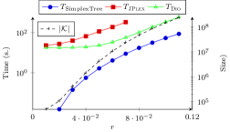
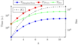
Figure 10. Statistics and timings for the construction of the Rips complex on (Left) Bud and (Right) Cy8.

We test our algorithm for the construction of Rips complexes. In Figure 10 we compare the performance of our algorithm with JPlex and with Dionysus along two directions.

In the first experiment, we build the Rips complex on $49,000$ points from the dataset Bud. Our construction is at least $36$ times faster than JPlex along the experiment, and several hundred times faster for small values of the parameter $r$. Moreover, JPlex is not able to handle the full dataset Bud nor big simplicial complexes due to memory allocation issues, whereas our method has no such problems. In our experiments, JPlex is not able to compute complexes of more than $23$ million faces ($r=0.07$) while the simplex tree construction runs successfully until $r=0.11$, resulting in a complex of $237$ million faces. Our construction is at least $7$ times faster than Dionysus along the experiment, and several hundred times faster for small values of the parameter $r$.

In the second experiment, we construct the Rips complex on the $6040$ points from Cy8, with threshold $r=0.4$, for different dimensions $k$. Again, our method outperforms JPlex, by a factor $11$ to $14$. JPlex cannot compute complexes of dimension higher than $7$ because it is limited by design to simplicial complexes of dimension smaller than $7$. Our construction is $4$ to $12$ times faster than Dionysus.

The simplex tree and the expansion algorithm we have described are output sensitive. As shown by our experiments, the construction time using a simplex tree depends linearly on the size of the output complex. Indeed, when the Rips graphs are dense enough so that the time for the expansion dominates the full construction, we observe that the average construction time per face is constant and equal to $3.7\times 10^{-7}$ seconds for the first experiment, and $4.1\times 10^{-7}$ seconds for the second experiment (with standard errors $0.20\%$ and $0.14\%$ respectively).

4.3. Construction of Witness Complexes

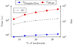
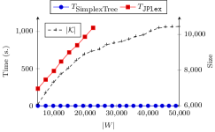
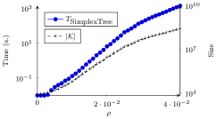
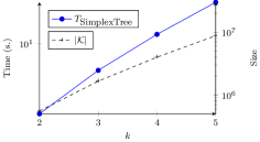
Figure 11. Statistics and timings for the construction of: (TOP) the witness complex and (BOTTOM) the relaxed witness complex, on datasets (Left) Bro and (Right) Kl.

We test our algorithms for the construction of witness complexes and relaxed witness complexes.

Figure 11 (top) shows the results of two experiments for the full construction of witness complexes. The first one compares the performance of the simplex tree algorithm and of JPlex on the dataset Bro consisting of $15,000$ points in dimension $\mathbb{R}^{25}$. Subsets of different size of landmarks are selected at random among the sample points. Our algorithm is from several hundred to several thousand times faster than JPlex (from small to big subsets of landmarks). Moreover, the simplex tree algorithm for the construction of the witness complex represent less than $1\%$ of the total time spent, when more than $99\%$ of the total time is spent computing the nearest neighbors of the witnesses.

In the second experiment, we construct the witness complex on $2,500$ landmarks from Kl, and sets of witnesses of different size. The simplex tree algorithm outperforms JPlex, being tens of thousands times faster. JPlex runs above the one hour time limit when the simplex tree algorithm stays under $0.1$ second all along the experiment. Moreover, the simplex tree algorithm spends only about $10\%$ of the time constructing the witness complex, and $90\%$ computing the nearest neighbors of the witnesses.

Finally we test the full construction of the relaxed witness complex. JPlex does not provide an implementation of the relaxed witness complex as defined in this paper; consequently, we were not able to compare the algorithms on the construction of the relaxed witness complex. We test our algorithms along two directions, as illustrated in Figure 11 (bottom). In the first experiment, we compute the $5$-skeleton of the relaxed witness complex on Bro, with $15,000$ witnesses and $1,000$ landmarks selected randomly, for different values of the parameter $\rho$. In the second experiment, we construct the $k$-skeleton of the relaxed witness complex on Kl with $10,000$ landmarks, $100,000$ witnesses and fixed parameter $\rho=0.07$, for various $k$. We are able to construct and store complexes of up to $260$ million faces. In both cases the construction time is linear in the size of the output complex, with a contruction time per face equal to $4.9\times 10^{-6}$ seconds in the first experiment, and $4.0\times 10^{-6}$ seconds in the second experiment (with standard errors $1.6\%$ and $6.3\%$ respectively).

Conclusion

We believe that the simplex tree is the first scalable and truly practical data structure to represent general simplicial complexes. The simplex tree is very flexible, can represent any kind of simplicial complexes and allow efficient implementations of all basic operations on simplicial complexes. Futhermore, since the simplex tree stores all simplices of the simplicial complex, it has been successfully applied to represent filtrations and to compute persistent homology [6]. We plan to make our code publicly available and to use it for practical applications in data analysis and manifold learning. Further developments also include more compact storage using succinct representations of trees [16].

Acknowledgements 4.1.

The authors thanks A.Ghosh, S. Hornus, D. Morozov and P. Skraba for discussions that led to the idea of representing simplicial complexes by tries. They especially thank S. Hornus for sharing his notes with us. They also thank S. Martin and V. Coutsias for providing the cyclo-octane data set. This research has been partially supported by the 7th Framework Programme for Research of the European Commission, under FET-Open grant number 255827 (CGL Computational Geometry Learning).

Appendix A Additional Experiments

In this section we provide more experiments on the running time of the algorithms for constructing Rips complexes and relaxed witness complexes on all datasets. The datasets used are described in Figure 8.

Bud:	$r$	$0.08$	$0.085$	$0.090$	$0.095$	$0.100$	$0.105$	$0.110$
	$T_{\text{Rips}}$	$19.4$	$26.5$	$35.8$	$46.7$	$60.5$	$77.7$	$98.7$
	$|\mathcal{K}|$	$69\cdot 10^{6}$	$94\cdot 10^{6}$	$127\cdot 10^{6}$	$167\cdot 10^{6}$	$217\cdot 10^{6}$	$280\cdot 10^{6}$	$355\cdot 10^{6}$
Bro:	$r$	$0.184$	$0.186$	$0.188$	$0.190$	$0.192$	$0.194$	$0.196$
	$T_{\text{Rips}}$	$15.3$	$18.1$	$28.2$	$34.5$	$40.8$	$56.2$	$81.1$
	$|\mathcal{K}|$	$52\cdot 10^{6}$	$61\cdot 10^{6}$	$95\cdot 10^{6}$	$117\cdot 10^{6}$	$138\cdot 10^{6}$	$190\cdot 10^{6}$	$275\cdot 10^{6}$
Cy8:	$r$	$0.406$	$0.415$	$0.424$	$0.433$	$0.442$	$0.451$	$0.460$
	$T_{\text{Rips}}$	$5.7$	$8.7$	$13.6$	$21.4$	$34.5$	$57.3$	$96.6$
	$|\mathcal{K}|$	$17\cdot 10^{6}$	$27\cdot 10^{6}$	$42\cdot 10^{6}$	$67\cdot 10^{6}$	$108\cdot 10^{6}$	$180\cdot 10^{6}$	$305\cdot 10^{6}$
Kl:	$r$	$0.059$	$0.062$	$0.065$	$0.068$	$0.071$	$0.074$	$0.077$
	$T_{\text{Rips}}$	$7.0$	$11.1$	$17.8$	$26.3$	$38.4$	$58.3$	$87.3$
	$|\mathcal{K}|$	$24\cdot 10^{6}$	$38\cdot 10^{6}$	$61\cdot 10^{6}$	$90\cdot 10^{6}$	$133\cdot 10^{6}$	$204\cdot 10^{6}$	$305\cdot 10^{6}$
S4:	$r$	$0.22$	$0.23$	$0.24$	$0.25$	$0.26$	$0.27$	$0.28$
	$T_{\text{Rips}}$	$2.7$	$4.7$	$8.5$	$15.4$	$28.0$	$50.9$	$93.7$
	$|\mathcal{K}|$	$7\cdot 10^{6}$	$13\cdot 10^{6}$	$23\cdot 10^{6}$	$43\cdot 10^{6}$	$79\cdot 10^{6}$	$146\cdot 10^{6}$	$271\cdot 10^{6}$

Figure 12. Timings $T_{\text{Rips}}$ for the construction of the Rips complex on the data sets and size of the simplicial complexes $|\mathcal{K}|$, for different values of the parameter $r$. On all these experiments, the time complexity is linear in the number of faces. Specifically, the timing per simplex ranges between $2.79\cdot 10^{-7}$ and $3.47\cdot 10^{-7}$ seconds per simplex depending on the dataset, with standard error at most $0.40\%$.

Bud:	$\rho$	$0.06$	$0.07$	$0.08$	$0.09$	$0.10$	$0.11$	$0.12$
	$T_{\mbox{$\mbox{{\rm Wit}}^{\rho}$}}$	$18.3$	$36.9$	$71.1$	$135.8$	$249.1$	$440.2$	$758.6$
	$|\mathcal{K}|$	$7.8\cdot 10^{6}$	$14\cdot 10^{6}$	$23\cdot 10^{6}$	$38\cdot 10^{6}$	$58\cdot 10^{6}$	$88\cdot 10^{6}$	$130\cdot 10^{6}$
Bro:	$\rho$	$0.0075$	$0.0080$	$0.0085$	$0.0090$	$0.0095$	$0.0100$	$0.0105$
	$T_{\mbox{$\mbox{{\rm Wit}}^{\rho}$}}$	$4.0$	$6.1$	$10.7$	$16.5$	$39.3$	$123.2$	$530.9$
	$|\mathcal{K}|$	$1.2\cdot 10^{6}$	$1.5\cdot 10^{6}$	$1.9\cdot 10^{6}$	$2.2\cdot 10^{6}$	$3.1\cdot 10^{6}$	$4.6\cdot 10^{6}$	$7.0\cdot 10^{6}$
Cy8:	$\rho$	$0.194$	$0.200$	$0.206$	$0.212$	$0.218$	$0.224$	$0.230$
	$T_{\mbox{$\mbox{{\rm Wit}}^{\rho}$}}$	$18.7$	$33.1$	$130.2$	$273.0$	$512.9$	$37.2$	$1411.2$
	$|\mathcal{K}|$	$0.45\cdot 10^{6}$	$0.66\cdot 10^{6}$	$0.82\cdot 10^{6}$	$1.1\cdot 10^{6}$	$1.7\cdot 10^{6}$	$2.3\cdot 10^{6}$	$3.6\cdot 10^{6}$
Kl:	$\rho$	$0.05$	$0.06$	$0.07$	$0.08$	$0.09$	$0.10$	$0.11$
	$T_{\mbox{$\mbox{{\rm Wit}}^{\rho}$}}$	$3.2$	$9.7$	$24.6$	$55.3$	$118.0$	$261.1$	$584.5$
	$|\mathcal{K}|$	$0.78\cdot 10^{6}$	$2.2\cdot 10^{6}$	$5.2\cdot 10^{6}$	$11\cdot 10^{6}$	$23\cdot 10^{6}$	$49\cdot 10^{6}$	$109\cdot 10^{6}$
S4:	$\rho$	$0.03$	$0.035$	$0.040$	$0.045$	$0.050$	$0.055$	$0.060$
	$T_{\mbox{$\mbox{{\rm Wit}}^{\rho}$}}$	$7.6$	$14.1$	$26.4$	$48.9$	$89.2$	$164.6$	$297.3$
	$|\mathcal{K}|$	$2.8\cdot 10^{6}$	$5.3\cdot 10^{6}$	$11\cdot 10^{6}$	$22\cdot 10^{6}$	$43\cdot 10^{6}$	$85\cdot 10^{6}$	$161\cdot 10^{6}$

Figure 13. Timings $T_{\text{$\mbox{{\rm Wit}}^{\rho}$}}$ for the construction of the relaxed witness complex on the data sets and size of the simplicial complexes $|\mathcal{K}|$, for different values of the parameter $\rho$. The timings per simplex vary, as the complexity of the construction algorithm depends also on the number of witnesses. It however ranges between $\approx 10^{-6}$ and $\approx 10^{-4}$ seconds per simplex depending on the number of witnesses compared to the number of simplices of the output.

References

- [1] The stanford 3d scanning repository. http://graphics.stanford.edu/data/3Dscanrep/.
- [2] Elke Achtert, Christian Böhm, Peer Kröger, Peter Kunath, Alexey Pryakhin, and Matthias Renz. Efficient reverse k-nearest neighbor search in arbitrary metric spaces. In SIGMOD Conference, pages 515–526, 2006.
- [3] Dominique Attali, André Lieutier, and David Salinas. Efficient data structure for representing and simplifying simplicial complexes in high dimensions. Int. J. Comput. Geometry Appl., 22(4):279–304, 2012.
- [4] Dominique Attali, André Lieutier, and David Salinas. Vietoris-rips complexes also provide topologically correct reconstructions of sampled shapes. Comput. Geom., 46(4):448–465, 2013.
- [5] Jon Louis Bentley and Robert Sedgewick. Fast algorithms for sorting and searching strings. In SODA, pages 360–369, 1997.
- [6] Jean-Daniel Boissonnat, Tamal K. Dey, and Clément Maria. The compressed annotation matrix: an efficient data structure for computing persistent cohomology. In ESA, 2013.
- [7] Jean-Daniel Boissonnat, Leonidas J. Guibas, and Steve Oudot. Manifold reconstruction in arbitrary dimensions using witness complexes. Discrete & Computational Geometry, 42(1):37–70, 2009.
- [8] Jean-Daniel Boissonnat and Clément Maria. The simplex tree: An efficient data structure for general simplicial complexes. In ESA, pages 731–742, 2012.
- [9] Jean-Daniel Boissonnat and Clément Maria. The simplex tree: An efficient data structure for general simplicial complexes. Algorithmica, 70(3):406–427, 2014.
- [10] Erik Brisson. Representing geometric structures in d dimensions: Topology and order. Discrete & Computational Geometry, 9:387–426, 1993.
- [11] Gunnar Carlsson, Tigran Ishkhanov, Vin de Silva, and Afra Zomorodian. On the local behavior of spaces of natural images. International Journal of Computer Vision, 76(1):1–12, 2008.
- [12] Frédéric Chazal and Steve Oudot. Towards persistence-based reconstruction in euclidean spaces. In SoCG, pages 232–241, 2008.
- [13] Vin de Silva and Gunnar Carlsson. Topological estimation using witness complexes. In Eurographics Symposium on Point-Based Graphics, 2004.
- [14] Tamal K. Dey, Fengtao Fan, and Yusu Wang. Computing topological persistence for simplicial maps. CoRR, abs/1208.5018, 2012.
- [15] Herbert Edelsbrunner and John Harer. Computational Topology - an Introduction. American Mathematical Society, 2010.
- [16] Guy Jacobson. Space-efficient static trees and graphs. In FOCS, pages 549–554, 1989.
- [17] Ann B. Lee, Kim Steenstrup Pedersen, and David Mumford. The nonlinear statistics of high-contrast patches in natural images. International Journal of Computer Vision, 54(1-3):83–103, 2003.
- [18] Pascal Lienhardt. N-dimensional generalized combinatorial maps and cellular quasi-manifolds. Int. J. Comput. Geometry Appl., 4(3):275–324, 1994.
- [19] Shawn Martin, Aidan Thompson, Evangelos .A. Coutsias, and Jean-Paul Watson. Topology of cyclo-octane energy landscape. J Chem Phys, 132(23):234115, 2010.
- [20] Dmitriy Morozov. Dionysus. http://www.mrzv.org/software/dionysus/.
- [21] David M. Mount and Sunil Arya. ANN, Approximate Nearest Neighbors Library. http://www.cs.sunysb.edu/ algorith/implement/ANN/implement.shtml.
- [22] Harlan Sexton and Mikael Vejdemo Johansson. JPlex, 2009. http://comptop.stanford.edu/programs/jplex/.
- [23] SGI. Standard template library programmer’s guide. http://www.sgi.com/tech/stl/.
- [24] Afra Zomorodian. The tidy set: a minimal simplicial set for computing homology of clique complexes. In SoCG, pages 257–266, 2010.