Correlated insulating phases of twisted bilayer graphene at commensurate filling fractions: A Hartree-Fock study

Abstract

Motivated by the recently observed insulating states in twisted bilayer graphene, we study the nature of the correlated insulating phases of the twisted bilayer graphene at commensurate filling fractions. We use the continuum model and project the Coulomb interaction onto the flat bands to study the ground states by using a Hartree-Fock approximation. In the absence of the hexagonal boron nitride substrate, the ground states are the intervalley coherence states at charge neutrality (filling $\nu$ = 0, or four electrons per moiré cell) and at $\nu$ = -1/4 and -1/2 (three and two electrons per cell, respectively) and the $C_{2}\mathcal{T}$ symmetry-broken state at $\nu$= -3/4 (one electron per cell). The hexagonal boron nitride substrate drives the ground states at all $\nu$ into $C_{2}\mathcal{T}$ symmetry broken-states. Our results provide good reference points for further study of the rich correlated physics in the twisted bilayer graphene.

I Introduction

The discovery of flat bands and superconductivity in twisted bilayer graphene (TBG) has promoted intensive investigations of the newly layered systems coupled by weak van der Waals interaction Cao et al. (2018a, b); Rozhkov et al. (2016). In analogy to high-temperature cuprates Lee et al. (2006), it was thought that superconductivity in TBG is closely related to the strongly correlated insulating phase at half filling Cao et al. (2018b). Insulating states (with and without hBN substrates alignment) have now also been observed in experiments at other fillings with integer number of electrons per moiré cell Sharpe et al. (2019); Serlin et al. (2019); Lu et al. (2019); Jiang et al. (2019); Kerelsky et al. (2019); Xie et al. (2019); Choi et al. (2019); Yankowitz et al. (2019). Many theories have been proposed to understand the superconductivity Po et al. (2018a); Isobe et al. (2018); Liu et al. (2018); Xu and Balents (2018); Wu et al. (2018); Lian et al. (2019); Huang et al. (2019); Kozii et al. (2019); Wu (2019); Roy and Juričić (2019); Tang et al. (2019) and the correlated insulating states Po et al. (2018a); Kang and Vafek (2019); Zhang et al. (2019); Isobe et al. (2018); Sboychakov et al. (2019); Xu et al. (2018); Huang et al. (2019); Xie and MacDonald (2020); Liu and Dai (2019); Liu et al. (2019); Bultinck et al. (2019); Rademaker et al. (2019); Wu and Das Sarma (2020); Guinea and Walet (2018); Seo et al. (2019). Theoretically, one can directly start from the tight-binding model in the original bilayer graphene lattice that captures the narrow bands, and add interaction to further study the correlating effects Sboychakov et al. (2019); Rademaker et al. (2019). Since the unit cell in such models contains tens of thousands of atoms, it can raise numerical difficulties when dealing with long-ranged Coulomb interaction. In order to overcome this difficulty, two kinds of methods are applied to construct the TBG effective models. One is to use the continuum model Bistritzer and MacDonald (2011); Lopes dos Santos et al. (2012) by scattering between Dirac points that belong to different layers. And the other is to construct tight-binding models from local Wannier orbitals Yuan and Fu (2018); Kang and Vafek (2018); Koshino et al. (2018); Po et al. (2019); Carr et al. (2019).

In this work, we use the continuum model Bistritzer and MacDonald (2011); Lopes dos Santos et al. (2012) to carry out a self-consistent mean-field study, which is equivalent to the Hartree-Fock approximation, for TBG commensurate fillings fractions corresponding to integer numbers of electrons per moiré cell. Due to particle-hole symmetry, we only need to consider fillings $\nu=-3/4$, $-1/2$, $-1/4$ and $0$ for one, two, three and four electrons occupying the 8 moiré flat bands, respectively. The ground states at positive fillings can be obtained by particle-hole symmetry. The flat bands are characterized by spin s, valley $\tau$ and band index m. In addition to the spin degrees of freedom, there are two sets of flat bands, which can be denoted as $\tau=\pm$ , resulted from the interlayer scattering of the states around the Dirac points at the graphene valley $K^{\pm}$, as shown in Fig.1(b).

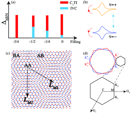
Figure 1: (a) Schematic phase diagram of TBG in the plane spanned by commensurate filling fraction and hBN potential $\Delta_{hBN}$. The red color stands for $C_{2}\mathcal{T}$ breaking insulator ($C_{2}\mathcal{T}$I) while the cyan for the intervalley coherent (IVC) state. (b) TBG contains two sets of flat bands from valley $\tau=+$ and $\tau=-$. IVC state is favored by the intervalley scattering (cyan arrow). The $C_{2}\mathcal{T}$I is favored by the interband scattering in each valley (red arrow). (c) Atomic structure of the TBG with twisted angle $\theta$=6.01^∘, where the red and blue dots represent the A, B sublattice. The AA region corresponds to the region where the two red dots from the two layers lie on top of each other while the AB and BA correspond to the region where the red and blue dots overlap with each other. (d) Schematic plot of the Brillouin zone folding in TBG, where the small hexagon represents the moiré Brillouin zone reciprocal to the moiré superlattice structure in (c). ${\mathbf{G}}_{1}$ and ${\mathbf{G}}_{2}$ are the reciprocal lattice vectors of the moiré Brillouin zone.

We project the Coulomb interaction between electrons into the flat band basis. This process is formally identical to the projection of the Coulomb interaction to the lowest Landau level in the fractional quantum Hall effect Haldane (1983). Then, we can apply a Hartree-Fock mean-field theory by decoupling the projected interactions into momentum dependent order parameters. The main results are summarized in Fig.1(a). There are mainly two kinds of states, intervalley coherence states (IVC) and the $C_{2}\mathcal{T}$ breaking states ($C_{2}\mathcal{T}$I). The intra-valley interband scattering favors $C_{2}\mathcal{T}$I (red arrow in Fig.1(b)) while the intervalley scattering favors IVC states (cyan arrow in Fig.1(b)). If the substrate potential $\Delta_{hBN}$=0, IVC states are found to be the ground state for $\nu=$ $-1/2$, $-1/4$ and $0$, while $C_{2}\mathcal{T}$I states are found to be the ground states for $\nu=$ -3/4. By increasing $\Delta_{hBN}$, $C_{2}\mathcal{T}$I states become more stable comparing to IVC states. Decreasing the bandwidth of the moiré bands reduces the energy difference between the IVC state and $C_{2}\mathcal{T}$I state, but does not affect the ground state until the moiré bands become completely flat where the two states are degenerate in energy.

Recently, the continuum model based Hartree-Fock approximation has been carried out by several groups. Xie et al. Xie and MacDonald (2020) and Liu et al. Liu and Dai (2019) have adopted the Hartree-Fock calculations that include flat bands as well as many remote bands to address the correlation and topological properties of TBG. Specificly, the latter introduces the momentum independent order parameters but studies more complete phase diagram at $\pm 1/2$ and $\pm 3/4$ fillings. Moreover Liu et al. Liu et al. (2019), Bultinck et al. Bultinck et al. (2019) have also applied a similar approximation by projecting the interactions to the lower energy bands to study the insulating phase at the charge neutral point.

This work is organized as follows. We start from the discussion of the continuum model and the Hartree-Fock mean-field formulation in Section II. In Section III, we discuss the main results at charge neutrality $\nu$=0, half-filling $\nu$=1/2 and $\nu$=3/4 filling. Then, we will briefly mention the results at $\nu$=1/4 filling and finalize the discussion in Section V.

II Formulation

II.1 moiré lattice structrue

The moiré pattern is formed by twisting the top and bottom layers of an aligned bilayer graphene by angles $\theta/2$ and $-\theta/2$. As shown in the panel (c) in Fig. 1, the formed periodic superlattice structure can be viewed as a triangular lattice of the AA region, where the atoms from the same sublattice of the two layers lie on top of each other with the lattice vectors $\mathbf{L_{M1}}=(0,-1)L_{M}$, $\mathbf{L_{M2}}=(\frac{\sqrt{3}}{2},-\frac{1}{2})L_{M}$ and $L_{M}=a_{0}/(2\sin(\theta/2))$, where $a_{0}$=0.246 nm, is the lattice constant of the monolayer graphene. The corresponding reciprocal lattice vectors of the moiré lattice are ${\mathbf{G}}_{1}=(-\frac{2\pi}{\sqrt{3L_{M}}},-\frac{2\pi}{L_{M}})$ and ${\mathbf{G}}_{2}=(-\frac{4\pi}{\sqrt{3L_{M}}},0)$. After the twisting, the momentum of the two Dirac points of the two layers becomes ${\mathbf{K}}_{1}^{\tau}$ and ${\mathbf{K}}_{2}^{\tau}$ and they are equivalent to the $-\tau{\mathbf{K}}_{1}$ and $-\tau{\mathbf{K}}_{2}$ in the moiré Brillouin zone as shown in Fig. 1(d).

II.2 Continuum model

The low energy physics of TBG can be described by the continuum model introduced by Bistritzer and MacDonald Bistritzer and MacDonald (2011); Lopes dos Santos et al. (2012). Here we formulate the continuum model as described by the Hamiltonian,

$$H^{\tau}_{BM}(\hat{\mathbf{k}})=\left(\begin{array}[]{cc}-\hbar v_{F}(\hat{{\mathbf{k}}}-{\mathbf{K}}_{1}^{\tau})\cdot\boldsymbol{\sigma}^{\tau}&U\\ U^{+}&-\hbar v_{F}(\hat{{\mathbf{k}}}-{\mathbf{K}}_{2}^{\tau})\cdot\boldsymbol{\sigma}^{\tau}\end{array}\right)$$ (1)

where $\tau=\pm$ is the valley index, $\boldsymbol{\sigma}^{\tau}=(\tau\sigma_{x},\sigma_{y})$ which is the Pauli matrices defined in the A,B sublattice space. ${\mathbf{K}}^{\tau}$ correspond to the two inequivalent Dirac points of the unrotated monolayer graphene, while ${\mathbf{K}}^{\tau}_{1}$ and ${\mathbf{K}}^{\tau}_{2}$ are the corresponding Dirac points of the bottom and top layers that are twisted by angles $\mp\frac{\theta}{2}$, and $\hat{{\mathbf{k}}}=-i\partial_{{\mathbf{r}}}$. The interlayer tunneling between the the Dirac states in the two layers is described by the matrix

$$\begin{split}U=&\left(\begin{array}[]{cc}u_{0}&u_{1}\\ u_{1}&u_{0}\end{array}\right)+\left(\begin{array}[]{cc}u_{0}&u_{1}e^{-\tau\frac{2\pi}{3}}\\ u_{1}e^{\tau\frac{2\pi}{3}}&u_{0}\end{array}\right)e^{-i\tau{\mathbf{G}}_{1}\cdot{\mathbf{r}}}\\ &+\left(\begin{array}[]{cc}u_{0}&u_{1}e^{\tau\frac{2\pi}{3}}\\ u_{1}e^{-\tau\frac{2\pi}{3}}&u_{0}\end{array}\right)e^{-i\tau({\mathbf{G}}_{1}+{\mathbf{G}}_{2})\cdot{\mathbf{r}}}\end{split}$$ (2)

where $u_{0}$ and $u_{1}$ are the intra-sublattice and inter-sublattice interlayer tunneling amplitudes. This continuum Hamiltonian is spin independent, so it has two SU(2) symmetries at each valley. Since it does not have terms that couple the two valleys, it also has a $U_{v}(1)$ for valley charge conservation in addition to the $U_{c}(1)$ for total charge conservation symmetry. Moreover, in the diagonal blocks of Eq. 1, we have neglected the rotation of the momentum $\hat{{\mathbf{k}}}-{\mathbf{K}}_{1,2}^{\tau}$ about the z axis for $\pm\theta/2$, due to its tiny effect for small twisted angle $\theta$, which leads to an additional particle-hole symmetry Bultinck et al. (2019); Liu and Dai (2019). We have checked that the inclusion of such symmetry breaking term will not affect the results of the paper. The eigenstate of $H_{BM}^{\tau}$ can be written in the Bloch wavefunction form

$$\psi_{m,\tau,{\mathbf{k}}}^{X}({\mathbf{r}})=\sum_{{\mathbf{G}}}u_{m,\tau;{\mathbf{G}},X}({\mathbf{k}})e^{i({\mathbf{k}}+{\mathbf{G}})\cdot{\mathbf{r}}}$$ (3)

where $X=\{A_{1},B_{1},A_{2},B_{2}\}$ is the layer and sublattice index with the eigen-energy $\epsilon_{m{\mathbf{k}}\tau}$. Here, m and $\tau$ are the band and valley indices and we omit the spin index s here since the Hamiltonian is spin independent. Throughout the paper, we fix the parameters as $\hbar v_{F}/a_{0}$=2.365 eV, the twist angle is fixed at $\theta$=1.086^∘. The inter-sublattice interlayer coupling is chosen as $u_{1}$=0.11 eV, so that the moiré bands are completely flat when the intra-sublattice interlayer coupling $u_{0}$ vanishes Tarnopolsky et al. (2019). In order to see the effect of moiré bandwidth, we tune the $u_{0}$ from the realistic value Carr et al. (2019); Nam and Koshino (2017) of 0.08 eV which corresponds to a bandwidth of 1.8 meV to the value of 0.01 eV resulting in a bandwidth of 0.03 meV.

II.3 Mean field theory

In order to study the effects of the Coulomb interaction, we apply our mean-field theory in the momentum space to decouple the interaction term. We solve a set of self-consistent equations to search for possible symmetry breaking states due to the Coulomb interaction. The mean-field calculation is performed in momentum space, which allows us to avoid the real space Wannier obstruction  Po et al. (2018a, b, 2019); Ahn et al. (2019). Moreover, in our calculation, we project the Coulomb interaction onto the two flat bands. More details of the projection to the flat bands are provided in appendix A.

After projecting onto the two flat bands, the total Hamiltonian becomes

$$\begin{split}H&=\sum_{m{\mathbf{k}}s\tau}(\epsilon_{m{\mathbf{k}}\tau}-\mu)d_{m{\mathbf{k}}s\tau}^{+}d_{m{\mathbf{k}}s\tau}\\ &+\frac{1}{2S}\sum_{\{m_{i}\}}\sum_{ss^{\prime}\tau\tau^{\prime}}\sum_{{\mathbf{k}}_{1}{\mathbf{k}}_{2}{\mathbf{q}}}V_{m_{1},m_{2},m_{3},m_{4}}^{\tau\tau^{\prime}\tau^{\prime}\tau}({\mathbf{k}}_{1},{\mathbf{k}}_{2},{\mathbf{q}})\\ &d_{m_{1}{\mathbf{k}}_{1}-{\mathbf{q}}s\tau}^{+}d_{m_{2}{\mathbf{k}}_{2}+{\mathbf{q}}s^{\prime}\tau^{\prime}}^{+}d_{m_{3}{\mathbf{k}}_{2}s^{\prime}\tau^{\prime}}d_{m_{4}{\mathbf{k}}_{1}s\tau}\end{split}$$ (4)

where S is the total area, $d^{+}_{m{\mathbf{k}}s\tau}$ and $d_{m{\mathbf{k}}s\tau}$ are the creation and annihilation operators in the projected flat band basis. Here, we neglect the intervalley interaction due to the Coulomb scattering between the two valleys $V({\mathbf{K}}^{+}-{\mathbf{K}}^{-})$ whose ratio to the intravalley interaction can be estimated by $a/L_{M}$ which is negligible for small twist angle. The projected interaction is derived from the Coulomb interaction $V({\mathbf{q}})$ as

$$\begin{split}&V_{m_{1},m_{2},m_{3},m_{4}}^{\tau\tau^{\prime}\tau^{\prime}\tau}({\mathbf{k}}_{1},{\mathbf{k}}_{2},{\mathbf{q}})=\sum_{{\mathbf{G}}}V({\mathbf{q}}+{\mathbf{G}})\\ &\lambda_{m_{1}m_{4};\tau}({\mathbf{k}}_{1}-{\mathbf{q}},{\mathbf{k}}_{1}+{\mathbf{G}})\lambda^{*}_{m_{3}m_{2};\tau^{{}^{\prime}}}({\mathbf{k}}_{2},{\mathbf{k}}_{2}+{\mathbf{q}}+{\mathbf{G}})\end{split}$$ (5)

where $\lambda_{m_{1}m_{2};\tau}({\mathbf{k}}_{1},{\mathbf{k}}_{2}+{\mathbf{G}})$ is the form factor written in terms of the Bloch wavefunction Eq. 3 as

$$\lambda_{m_{1}m_{2};\tau}({\mathbf{k}}_{1},{\mathbf{k}}_{2}+{\mathbf{G}})=\sum_{{\mathbf{G}}^{{}^{\prime}},X}u^{*}_{m_{1},\tau;{\mathbf{G}}^{{}^{\prime}},X}({\mathbf{k}}_{1})u_{m_{2},\tau;{\mathbf{G}}+{\mathbf{G}}^{{}^{\prime}},X}({\mathbf{k}}_{2})$$ (6)

We take $V({\mathbf{q}})$ as the single-gate-screened Coulomb potential Liu et al. (2019); Bultinck et al. (2019)

$$V({\mathbf{q}})=\frac{e^{2}}{2\varepsilon\varepsilon_{0}q}(1-e^{-2qd_{s}})$$ (7)

In this paper, we take the dielectric constant $\varepsilon=7$ and the gate distance $d_{s}=40$ nm. We have also checked the results using other sets of parameters and it will not change the ground state of the system.

Next, we perform a standard self-consistent mean-field calculation on Eq. 4. Since we only consider the states that preserve the translation symmetry at the scale of moiré unit cell, the mean-field order parameters are then defined by the density matrix $\rho({\mathbf{k}})$ whose elements are

$$\rho({\mathbf{k}})_{m_{1},s\tau;m_{2},s^{\prime}\tau^{\prime}}=\left<d_{m_{1}{\mathbf{k}}s\tau}^{+}d_{m_{2}{\mathbf{k}}s^{\prime}\tau^{\prime}}\right>$$ (8)

Since this density matrix is finite even for the nonsymmetry breaking states in the charge channel, which will be double-counted when coupled to the density operators in the mean-field Hamiltonian, we need to remove these double counting terms in the calculation. Different approaches have been used to address this issue Xie and MacDonald (2020); Liu et al. (2019); Bultinck et al. (2019). Here we take care of this by subtracting the density matrix of the nonsymmetry breaking states $\rho_{0}({\mathbf{k}})$ at the filling studied from $\rho({\mathbf{k}})$, so that there is always a trivial solution from the mean-field Hamiltonian which corresponds to the fully symmetric state. This means the density matrix that couples to the density operator in the mean-field Hamiltonian is effectively $\rho({\mathbf{k}})-\rho_{0}({\mathbf{k}})$. More details of the mean-field approximation are provided in appendix B. At charge neutrality, our approach is equivalent to that used in Ref. Liu et al., 2019.

III Results

We have applied the self-consistent mean-field calculation to different integer fillings, and find several symmetry breaking gapped states induced by the interaction.

III.1 $\nu=0$ case

At the charge neutral point, there are four electrons occupying the eight moiré bands. The self-consistent mean-field calculation leads to several symmetry breaking insulating states which can be classified into three groups according to the specific symmetry that is broken in these states. The first group is the flavor-polarized states including spin-polarized (SP), valley-polarized (VP) and spin-valley locked (SV) states which either break $SU(2)$ symmetry or spinless time reversal symmetry $\mathcal{T}$ or both. These states are generalized ferromagnetic insulating states (FMI). If we let $s$, $\tau$ and $\gamma$ be the Pauli matrices in the spin, valley and band basis the order parameter of the FM states can be written as $s_{z}\tau_{0}\gamma_{0}$, $s_{0}\tau_{z}\gamma_{0}$ or $s_{z}\tau_{z}\gamma_{0}$ and these states are degenerate in energy. The second group includes the insulating states that break $C_{2}\mathcal{T}$ symmetry and is labeled by $C_{2}\mathcal{T}$I, where the Dirac points are completely gapped out due to the $C_{2}\mathcal{T}$ breaking. Their order parameter is dominated by the term $s_{0,z}\tau_{0,z}\gamma_{x}$. They are also degenerate in energy. The last group is the intervalley coherent (IVC) state, which mixes the states from the two opposite valleys so that the $U_{v}(1)$ valley charge convervation is broken. The order parameter associated with this state can be written as $s_{0,z}\tau_{x,y}\gamma_{y}$.

In order to determine which state is the ground state, we calculate the total energy per particle for each mean-field solution. As shown in Fig. 2, the IVC state is always the ground state. For realistic parameters, where the intra-sublattice interlayer coupling $u_{0}$=0.08 eV, the IVC state is about 1 meV lower than the $C_{2}\mathcal{T}$I and FMI states. As $u_{0}$ decreases from 0.08 eV to 0.01 eV, where the bandwidth of the non-interaction moiré bands becomes flatter and flatter, the energy of $C_{2}\mathcal{T}$I becomes closer and closer in energy to the IVC state. These results are consistent with those of Ref. Liu et al., 2019; Bultinck et al., 2019. The IVC has an energy gap of about 40 meV as shown in the panel (b) in Fig. 2. Panel (c) shows one of the (VP) FMI states where all the four bands have double spin degeneracy. Panel (d) shows one of the $C_{2}\mathcal{T}$I states with order $s_{0}\tau_{0}\gamma_{x}$, which has an energy gap of about 35.5 meV.

We have also studied the effect of sublattice potential, which is associated with the alignment of the hBN substrate with one of the graphene layers. This staggered potential can be formulated by an extra term $\Delta_{hBN}\sigma_{z}$ adding to Eq. 1. We find that the IVC state is quickly suppressed by the staggered potential and the ground state then becomes the $C_{2}\mathcal{T}$I. This is understandable since the stagered potential explicitly breaks the $C_{2}$ sublattice symmetry, which should favor the $C_{2}\mathcal{T}$ breaking state.

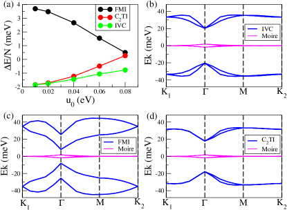
Figure 2: (a) Total energy per particle for ferromagnetic insulator (FMI), $C_{2}\mathcal{T}$ breaking insulator ($C_{2}\mathcal{T}$I) and intervalley coherent (IVC) states at the charge neutrality for various values of the intra-sublattice interlayer coupling $u_{0}$, where we choose $\Delta E$ to be relative to the average energy of these three states to clarify the small energy difference. (b)(c)(d) Typical energy dispersion of states of these three groups of states, where $u_{0}$=0.08 eV and the chemical potential is moved to the center of the gap for convenience. The non-interaction bands calculated from the $H_{BM}$ are also plotted for comparison.

III.2 $\nu=-\frac{1}{2}$ case

At the half filling case, there are two or six electrons occupying the eight moiré bands. Since these two cases are related by particle-hole transformation, we only consider the case with two electrons, i.e. $\nu$=-1/2. Similarly, the self-consistent mean-field calculation gives three groups of states which can be viewed as the flavor-polarized version of those states found at the charge neutral case.

The first group of states is the fully flavor-polarized states that do not mix the two moiré bands. Since there are only two electrons occupying the eight bands, only one of the four spin-valley combined flavors is fully filled leaving the other three completely empty. We again call this group of states as FMI and the order parameter of FMI can be described by the term $(s_{0}\pm s_{z})(\tau_{0}\pm\tau_{z})\gamma_{0}$ depending on which combination of flavors is fully filled. As shown in panel (c) in Fig. 3, the two filled bands below the chemical potential correspond to the two bands of the ordered flavor, and since $C_{2}\mathcal{T}$ symmetry is not broken, the Dirac points for each flavor are not destroyed. One set of the occupied bands is double degenerate corresponding to the spin degeneracy of the opposite valley of the filled bands. The energy gap of these states is about 18.7 meV. The second group of states includes the spin or valley polarized states that also mixes the two moiré bands, so we name them as the $C_{2}\mathcal{T}$FMI states. The order parameter of these states can be described by the terms as $(s_{0}\pm s_{z})\tau_{0,z}\gamma_{x}$ for the spin-polarized states and $s_{0,z}(\tau_{0}\pm\tau_{z})\gamma_{x}$ for the valley-polarized states. The $C_{2}\mathcal{T}$ symmetry is always broken in the polarized species (spin or valley) and preserved in the other. As shown in the panel (d) in Fig. 3 which corresponds to the valley-polarized $C_{2}\mathcal{T}$FMI, the Dirac points are indeed gapped out in the filled bands, while those in the unoccupied bands are not destroyed. The energy gap in these states is about 25.5 meV. The third group of states is the spin-polarized IVC states, which mixes the two valleys for one spin component. Its order parameter can be described by the terms as $(s_{0}\pm s_{z})\tau_{x,y}\gamma_{y}$. The energy dispersion of this IVC state is shown in the panel (b) in Fig. 3, whose energy gap is about 28.6 meV.

By comparing the total energy per particle of the states in each group, we again find that the ground state is the IVC state. The energy of the IVC states is lower by 0.5 meV at $u_{0}$=0.08 eV and approaches the $C_{2}\mathcal{T}$FMI as the bandwidth of the moiré bands decreases by tuning down $u_{0}$.

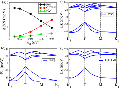
Figure 3: (a) Total energy per particle for ferromagnetic insulator (FMI), flavor polarized $C_{2}\mathcal{T}$ breaking insulator ($C_{2}\mathcal{T}$FMI) and intervalley coherent (IVC) states at half filling for various values of the intra-sublattice interlayer coupling $u_{0}$, where we choose $\Delta E$ to be relative to the average energy of these three states to clarify the small energy difference. (b)(c)(d) Typical energy dispersion of states of these three groups of states, where $u_{0}$=0.08 eV and the chemical potential is moved to the center of the gap for convenience.

We have also studied the effect of staggered potential at this filling and we find that by adding the staggered potential $\Delta_{hBN}\sigma_{z}$, the IVC ground state starts to mix with the $C_{2}\mathcal{T}$ breaking order, and the IVC order parameter is quickly suppressed as $\Delta_{hBN}$ reaches 0.3 meV, so that the ground state becomes the $C_{2}\mathcal{T}$FMI. The evolution of the two order parameters is shown in the panel (a) in Fig. 4.

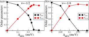
Figure 4: Evolution of the intervalley coherent (IVC) state and $C_{2}\mathcal{T}$ breaking order parameters with the increasing of the staggered potential $\Delta_{hBN}$ for $u_{0}$=0.08 eV at (a) half filling $\nu=-1/2$ and (b) quarter filling $\nu$=-1/4.

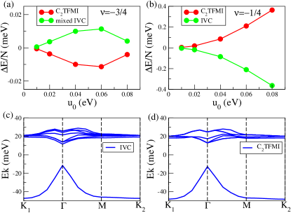
Figure 5: Total energy per particle for flavor-polarized C${}_{2}\mathcal{T}$ breaking insulator (C${}_{2}\mathcal{T}$FMI) and mixed intervalley coherent (IVC) states at $\nu=-\frac{3}{4}$ (a) and $\nu=-\frac{1}{4}$ (b) for various values of the intra-sublattice interlayer coupling $u_{0}$, where we choose $\Delta E$ to be relative to the average energy of these two states to clarify the small energy difference. (c)(d) Typical energy dispersion of states of these two groups of states, where $u_{0}$=0.08 eV and the chemical potential is moved to the center of the gap for convenience.

III.3 $\nu=-\frac{3}{4}$ case

At the case $\nu=\pm\frac{3}{4}$, there are one or seven electrons occupying the eight moiré bands. Again, since these two cases are related by particle-hole transformation, we only consider the case with one electron, i.e. $\nu=-\frac{3}{4}$. In this filling, the self-consistent mean-field calculation leads to two gapped solutions, including the flavor-polarized $C_{2}\mathcal{T}$FMI and a mixed order state with both IVC order parameter and $C_{2}\mathcal{T}$ breaking order parameter. This time, the energy of these two states are very close to each other and $C_{2}\mathcal{T}$FMI is lower in energy by at most 0.022 meV for various values of $u_{0}$ from 0.01 eV to 0.08 eV, as shown in the panel (a) in Fig. 5. For the realistic case where $u_{0}$=0.08 meV, energy gap is about 25.6 meV and for the $C_{2}\mathcal{T}$FMI state and 23.1 meV for the mixed IVC state as shown in the panel (c) and (d) in Fig. 5. The IVC component of the order parameter of the mixed IVC state will be quickly suppressed if there is a small staggered potential arising from the alignment of the hBN substrate and the ground state is $C_{2}\mathcal{T}$FMI which is the QAH states reported in the experiment Serlin et al. (2019); Sharpe et al. (2019).

III.4 $\nu=-\frac{1}{4}$ case

Again we consider only the hole dope side $\nu=-\frac{1}{4}$, i.e. there are three electrons occupying the eight moiré bands. We also find two groups of states in this case, which are the $C_{2}\mathcal{T}$FMI state and the IVC state. In the $C_{2}\mathcal{T}$FMI state, three out of the four spin-valley flavors are occupied while the other flavor is completely empty. Within each filled flavor, the two flat bands are mixed so that $C_{2}\mathcal{T}$ is breaking and an energy gap of about 25.7 meV is opened. The IVC state also only involves three flavors, while two of them with the same spin and opposite valleys form an IVC state by mixing the two opposite valleys, the other flavor form a $C_{2}\mathcal{T}$ breaking order by mixing the two flat bands within that flavor, so the IVC state at this filling can also be viewed as the mixed order of the IVC and $C_{2}\mathcal{T}$ order and the energy gap of this state is about 25.7 meV. Comparing the energy of the two groups of states, we find that IVC state is always the ground state and the energy difference from the $C_{2}\mathcal{T}$FMI also decreases with the decreasing of the bandwidth as shown in the panel (b) in Fig. 5. Similarly, if we add a small staggered potential $\Delta_{hBN}$, the IVC order will be suppressed quickly as shown in the panel (b) in Fig. 4.

IV Comparisons to other works

In this section, we compare our method and results to the other recent works that also aim at understanding the Hartree-Fock ground states in twisted bilayer graphene Liu et al. (2019); Bultinck et al. (2019); Liu and Dai (2019); Xie and MacDonald (2020). Ref. 28 and 29 performed the Hartree-Fock calculations including all remote bands without projecting to the low energy flat bands. This embraces the full complexity of the band structure, and simplifications were made in treating the effects of the Coulomb interaction at the Hartree-Fock level. In our calculation, we project the Coulomb interaction onto the lowest two flat bands per spin and valley, and treat the correlation effect at the Hartree-Fock level more completely. As a consequence, the results we obtained are very different from those of Ref. 28 and Ref. 29. Specifically, Ref. 28 mainly focused on whether the $C_{2}\mathcal{T}$ symmetry is broken and completely ignored the IVC state, which we find to be the energetically more favorable ground state at the charge neutral 0, 1/2, and 1/4 fillings. In Ref. 29, the IVC and all order parameters were considered, but an approximation was made to assume that the Fock term is momentum independent. This approximation may lead to different results at the studied 1/2 and 3/4 fillings compared to our results. For 1/2 filling, we find the ground state is the insulating IVC state consistent with the analytic argument given in Ref. 31, whereas the results in Ref. 29 indicate either an IVC or a valley polarized state or even a coexistence of them as the ground states, which can be either insulating or metallic depending on the screening length and the dielectric constant. For 3/4 filling, our results show an insulating IVC ground state with a finite gap, while the results of Ref. 29 show a metallic state. Since the recent experimental work Lu et al. (2019) found that at both 1/2 and 3/4 fillings, the ground state is always an insulating state without hBN alignment, the results obtained here are more in-line with the experiments, suggesting that projection the Coulomb interaction to the lowest flat bands followed by a more complete Hartree-Fock treatment of the correlation effects may capture the low energy physics properly.

The method of projecting the interaction to the low energy flat bands was independently developed in Refs. 30 and 31 to study the charge neutral point at the HF level. Specifically, Ref. 30 projected the Coulomb interaction to the lowest two flat bands, the same as in our approach. However, we found a lower energy ground state, i.e. the IVC state, which was not considered in the calculations of Ref. 30.

In Ref. 31, the authors projected the Coulomb interaction onto the lowest six bands per spin and valley, and included the IVC state, which was indeed found to be the ground state in their calculations at the charge neutral point. Our results at the charge neutral point is indeed consistent with Ref. 31. For example, the energy gap for the IVC states in our approach is $\Delta_{IVC}=35.5$ meV. The average energies of the IVC and $C_{2}\mathcal{T}$I states are $E_{IVC}=-21.4$ meV and $E_{C_{2}\mathcal{T}I}=-20.3$ meV, respectively, implying the IVC state is lower in energy by $1.1$ meV. These results are numerically consistent with those reported in Figs.7(c,d) of Ref. 31, and further indicating that the low energy physics can be captured by projecting the the two lowest flat bands.

The other new result of our work, which is complementary to Ref. 30 and 31, is that we have systematically and quantitatively studied the HF ground states at other commensurate fillings beyond the charge neutron point. This required a generalization of the subtraction scheme to deal with the double counting in the HF calculations introduced in Ref. 30 to ensure the existence of a trivial solution without any symmetry breaking at all commensurate fillings, with the details provided in appendix B. At 1/2 filling, our numerical calculations show that ground state is the spin-polarized IVC state, which is consistent with the analytic argument (explicit calculations were not performed) given in Ref. Bultinck et al., 2019. These agreements at both charge neutral and 1/2 filling not only benchmark our method but also attest the picture that the two emergent flat bands near the magic angle play the most important role, and projecting the Coulomb interaction onto them can determine the ground state properties. The latter may offer a useful framework for implementing more accurate, but numerically costly many-body studies beyond the Hartree-Fock approximation in the future. Moreover, we also obtained the HF ground states at 1/4 and 3/4 fillings, which were not studied in Ref. 31. Finally, the insulating ground states obtained in our calculations at 1/2 and 3/4 fillings are consistent with recent experiments Lu et al. (2019) as discussed above.

V Conclusion

In conclusion, we have performed self-consistent mean-field calculations at commensurate filling fractions of the twisted bilayer graphene around the magic angle. We find insulating ground states for all these fillings, which is consistent with the experimental results. For $\nu=0$, $-\frac{1}{2}$ and $-\frac{1}{4}$, the ground state is the intervalley coherent (IVC) state, and for $-\frac{3}{4}$ filling, the ground state is the flavor-polarized $C_{2}\mathcal{T}$ breaking insulator ($C_{2}\mathcal{T}$FMI). The energy difference between the IVC state and the $C_{2}\mathcal{T}$I state decreases as the bandwidth of the flat bands decreases. A small staggered potential associated with the hBN alignment can quickly suppressed the IVC order and stabilize the $C_{2}\mathcal{T}$ breaking state for all the fillings.

We have also checked the effect of screening strength by tuning the gate distance $d_{s}$ in Eq. 7 from 40 nm down to 5 nm. The screening strength is stronger as $d_{s}$ decreases which makes the Coulomb interaction more short-ranged. We find that as $d_{s}$ decreases, the total energy of all the mean-field states increases while their energy differences do not change sign, i.e no phase transition occurs. The increase of the energy is due to the fact that the stronger screening reduces the magnitude of the Coulomb interaction therefore reduces the energy gain of the mean-field solution. An example plot for the case with $\nu=-\frac{1}{2}$ is provided in the appendix C.

Acknowledgments– This work is in part supported by the National Natural Science Foundation of China No. 11674278 (YZ and FZ) and the U.S. Department of Energy, Basic Energy Sciences Grant No. DE-FG02-99ER45747 (KJ and ZW).

Appendix A Projection to the flat bands

The Bloch wavefunction calculated from the continuum model has the following form:

$$\psi_{n,\tau,{\mathbf{k}}}^{X}({\mathbf{r}})=\sum_{{\mathbf{G}}}u_{n,\tau;{\mathbf{G}},X}({\mathbf{k}})e^{i({\mathbf{k}}+{\mathbf{G}})\cdot{\mathbf{r}}}$$ (9)

where $X=A_{1},B_{1},A_{2},B_{2}$ corresponds to the mixture of sublattice and layer indices and ${\mathbf{G}}$ is the reciprocal lattice in the morie Brillouin zone expressed as ${\mathbf{G}}=n_{1}{\mathbf{G}}_{1}+n_{2}{\mathbf{G}}_{2}$. Here, we use 121 ${\mathbf{G}}$ vectors with $n_{1},n_{2}\in[-5,5]$ which is enough to produce the flat band. Eq. 9 provides the transformation between the original monolayer graphene operators $c^{+}$, $c$ and the operators in the projected eigenbasis $d^{+}$, $d$ which reads:

$$c_{X,{\mathbf{k}}+{\mathbf{G}},s\tau}=\sum_{n}u_{n,\tau;{\mathbf{G}},X}({\mathbf{k}})d_{n,{\mathbf{k}},s\tau}$$ (10)

where the momentum of $c$ operator is defined in the big Brillouin Zone (BZ) of the monolayer graphene while the momentum of the operator $d$ is defined in the moiré Brillouin Zone (mBZ), with the periodic boundary condition $d_{n,{\mathbf{k}}+{\mathbf{G}},s\tau}=d_{n,{\mathbf{k}},s\tau}$ Then the interaction part of the Hamiltonian is

$$\begin{split}H_{int}&=\frac{1}{2S}\sum_{X,X^{\prime},ss^{\prime},\tau\tau^{\prime}}\sum_{\tilde{{\mathbf{k}}}_{1}\tilde{{\mathbf{k}}}_{2}\tilde{{\mathbf{q}}}\in\text{BZ}}V^{XX^{\prime}}(\tilde{{\mathbf{q}}})c_{X,\tilde{{\mathbf{k}}}_{1}-\tilde{{\mathbf{q}}}s\tau}^{+}c_{X^{\prime},\tilde{{\mathbf{k}}}_{2}+\tilde{{\mathbf{q}}}s^{\prime}\tau^{\prime}}^{+}c_{X^{\prime},\tilde{{\mathbf{k}}}_{2}s^{\prime}\tau^{\prime}}c_{X,\tilde{{\mathbf{k}}}_{1}s\tau}\\ &=\frac{1}{2S}\sum_{m_{1},m_{2},m_{3},m_{4}}\sum_{{\mathbf{k}}_{1}{\mathbf{k}}_{2}{\mathbf{q}}\in\text{mBZ}}\sum_{{\mathbf{G}}_{1}{\mathbf{G}}_{2}{\mathbf{G}}}\sum_{X,X^{\prime},ss^{\prime},\tau\tau^{\prime}}V({\mathbf{q}}+{\mathbf{G}})u^{*}_{m_{1},\tau;{\mathbf{G}}_{1}-{\mathbf{G}},X}({\mathbf{k}}_{1}-{\mathbf{q}})u^{*}_{m_{2},\tau^{\prime};{\mathbf{G}}_{2}+{\mathbf{G}},X^{\prime}}({\mathbf{k}}_{2}+{\mathbf{q}})\\ &u_{m_{3},\tau^{\prime};{\mathbf{G}}_{2},X^{\prime}}({\mathbf{k}}_{2})u_{m_{4},\tau;{\mathbf{G}}_{1},X}({\mathbf{k}}_{1})d_{m_{1}{\mathbf{k}}_{1}-{\mathbf{q}}s\tau}^{+}d_{m_{2}{\mathbf{k}}_{2}+{\mathbf{q}}s^{\prime}\tau^{\prime}}^{+}d_{m_{3}{\mathbf{k}}_{2}s^{\prime}\tau^{\prime}}d_{m_{4}{\mathbf{k}}_{1}s\tau}\\ &=\frac{1}{2S}\sum_{m_{1},m_{2},m_{3},m_{4}}\sum_{{\mathbf{k}}_{1}{\mathbf{k}}_{2}{\mathbf{q}}\in\text{mBZ}}\sum_{{\mathbf{G}},ss^{\prime},\tau\tau^{\prime}}V({\mathbf{q}}+{\mathbf{G}})\lambda_{m_{1}m_{4};\tau}({\mathbf{k}}_{1}-{\mathbf{q}},{\mathbf{k}}_{1}+{\mathbf{G}})\lambda^{*}_{m_{3}m_{2};\tau^{{}^{\prime}}}({\mathbf{k}}_{2},{\mathbf{k}}_{2}+{\mathbf{q}}+{\mathbf{G}})\\ &d_{m_{1}{\mathbf{k}}_{1}-{\mathbf{q}}s\tau}^{+}d_{m_{2}{\mathbf{k}}_{2}+{\mathbf{q}}s^{\prime}\tau^{\prime}}^{+}d_{m_{3}{\mathbf{k}}_{2}s^{\prime}\tau^{\prime}}d_{m_{4}{\mathbf{k}}_{1}s\tau}\\ &=\frac{1}{2S}\sum_{m_{1},m_{2},m_{3},m_{4}}\sum_{{\mathbf{k}}_{1}{\mathbf{k}}_{2}{\mathbf{q}}\in\text{mBZ}}\sum_{ss^{\prime},\tau\tau^{\prime}}V^{\tau\tau^{\prime}\tau^{\prime}\tau}_{m_{1},m_{2},m_{3},m_{4}}({\mathbf{k}}_{1},{\mathbf{k}}_{2},{\mathbf{q}})d_{m_{1}{\mathbf{k}}_{1}-{\mathbf{q}}s\tau}^{+}d_{m_{2}{\mathbf{k}}_{2}+{\mathbf{q}}s^{\prime}\tau^{\prime}}^{+}d_{m_{3}{\mathbf{k}}_{2}s^{\prime}\tau^{\prime}}d_{m_{4}{\mathbf{k}}_{1}s\tau}\end{split}$$ (11)

where we use the single-gate-screened Coulomb potential to approximate the interaction $V^{XX^{\prime}}({\mathbf{q}})$ as

$$V^{XX^{\prime}}({\mathbf{q}})=V({\mathbf{q}})=\frac{e^{2}}{2\varepsilon\varepsilon_{0}q}(1-e^{-2qd_{s}})$$ (12)

and $\lambda_{m_{1}m_{2};\tau}({\mathbf{k}}_{1},{\mathbf{k}}_{2}+{\mathbf{G}})$ is the form factor defined by the Bloch wavefunction as

$$\lambda_{m_{1}m_{2};\tau}({\mathbf{k}}_{1},{\mathbf{k}}_{2}+{\mathbf{G}})=\sum_{{\mathbf{G}}^{{}^{\prime}},X}u^{*}_{m_{1},\tau;{\mathbf{G}}^{{}^{\prime}},X}({\mathbf{k}}_{1})u_{m_{2},\tau;{\mathbf{G}}+{\mathbf{G}}^{{}^{\prime}},X}({\mathbf{k}}_{2})$$ (13)

so that the projected Coulomb interaction matrix is

$$V^{\tau\tau^{\prime}\tau^{\prime}\tau}_{m_{1},m_{2},m_{3},m_{4}}({\mathbf{k}}_{1},{\mathbf{k}}_{2},{\mathbf{q}})=\sum_{{\mathbf{G}}}V({\mathbf{q}}+{\mathbf{G}})\lambda_{m_{1}m_{4};\tau}({\mathbf{k}}_{1}-{\mathbf{q}},{\mathbf{k}}_{1}+{\mathbf{G}})\lambda^{*}_{m_{3}m_{2};\tau^{{}^{\prime}}}({\mathbf{k}}_{2},{\mathbf{k}}_{2}+{\mathbf{q}}+{\mathbf{G}})$$ (14)

The form factor $\lambda_{m_{1}m_{2};\tau}({\mathbf{k}}_{1},{\mathbf{k}}_{2}+{\mathbf{G}})$ satisies the following two equation as:

$$\lambda_{m_{1}m_{2};\tau}({\mathbf{k}}_{1},{\mathbf{k}}_{2}+{\mathbf{G}})=\lambda^{*}_{m_{2}m_{1};\tau}({\mathbf{k}}_{2},{\mathbf{k}}_{1}-{\mathbf{G}})$$ (15)

from the definition, and

$$\lambda_{m_{1}m_{2};-\tau}({\mathbf{k}}_{1},{\mathbf{k}}_{2}+{\mathbf{G}})=\lambda^{*}_{m_{1}m_{2};\tau}(-{\mathbf{k}}_{1},-{\mathbf{k}}_{2}-{\mathbf{G}})$$ (16)

due to the time reversal symmetry.

Appendix B Mean-field approximation

In the section above, we have derived the Eq. 4 and  5 in the main text. We use the self-consistent HF approximation to decouple the interaction term. Using the order parameter defined in Eq. 8

$$\rho({\mathbf{k}})_{m_{1},s\tau;m_{2},s^{\prime}\tau^{\prime}}=\left<d_{m_{1}{\mathbf{k}}s\tau}^{+}d_{m_{2}{\mathbf{k}}s^{\prime}\tau^{\prime}}\right>$$

where we have confined the order the direction for spin in z-axis, which will not affect the general conclusion of the ground state, the interaction term becomes:

$$\begin{split}H_{HF}&=\frac{1}{2S}\sum_{\{m_{i}\}}\sum_{ss^{\prime}\tau\tau^{\prime}}\sum_{{\mathbf{k}}_{1}{\mathbf{k}}_{2}}V_{m_{1}m_{2}m_{3}m_{4}}^{\tau\tau^{\prime}\tau^{\prime}\tau}({\mathbf{k}}_{1},{\mathbf{k}}_{2},0)[\rho({\mathbf{k}}_{1})_{m_{1},s\tau;m_{4},s\tau}d_{m_{2}{\mathbf{k}}_{2}s^{\prime}\tau^{\prime}}^{+}d_{m_{3}{\mathbf{k}}_{2}s^{\prime}\tau^{\prime}}\\ &+\rho({\mathbf{k}}_{2})_{m_{2},s^{\prime}\tau^{\prime};m_{3},s^{\prime}\tau^{\prime}}d_{m_{1}{\mathbf{k}}_{1}s\tau}^{+}d_{m_{4}{\mathbf{k}}_{1}s\tau}-\rho({\mathbf{k}}_{1})_{m_{1},s\tau;m_{4},s\tau}\rho({\mathbf{k}}_{2})_{m_{2},s\tau;m_{3},s^{\prime}\tau^{\prime}}]\\ &-\frac{1}{2S}\sum_{\{m_{i}\}}\sum_{s\tau}\sum_{{\mathbf{k}}_{1}{\mathbf{k}}_{2}}V_{m_{1}m_{2}m_{3}m_{4}}^{\tau\tau^{\prime}\tau^{\prime}\tau}({\mathbf{k}}_{1},{\mathbf{k}}_{2},{\mathbf{k}}_{1}-{\mathbf{k}}_{2})[\rho({\mathbf{k}}_{2})_{m_{1},s\tau;m_{3},s\tau^{\prime}}d_{m_{2}{\mathbf{k}}_{1}s\tau^{\prime}}^{+}d_{m_{4}{\mathbf{k}}_{1}s\tau}\\ &+\rho({\mathbf{k}}_{1})_{m_{2},s\tau^{\prime};m_{4},s\tau}d_{m_{1}{\mathbf{k}}_{2}s\tau}^{+}d_{m_{3}{\mathbf{k}}_{2}s\tau^{\prime}}-\rho({\mathbf{k}}_{2})_{m_{1},s\tau;m_{3},s\tau^{\prime}}\rho({\mathbf{k}}_{1})_{m_{2},s\tau^{\prime};m_{4},s\tau}]\\ &=\sum_{{\mathbf{k}}s\tau\tau^{\prime}}\sum_{m_{1}m_{2}}h_{m_{1},\tau;m_{2},\tau^{\prime},{\mathbf{k}}s}d_{m_{1}{\mathbf{k}}s\tau}^{+}d_{m_{2}{\mathbf{k}}s\tau^{\prime}}-E_{c}\end{split}$$ (17)

where,

$$\begin{split}h_{m_{1},\tau;m_{2},\tau^{\prime},{\mathbf{k}}s}&=\frac{1}{2S}\sum_{m_{1}^{\prime}m_{2}^{\prime}{\mathbf{k}}^{\prime}}\{\sum_{s^{\prime}\tau^{\prime\prime}}[V_{m_{1}^{\prime}m_{1}m_{2}m_{2}^{\prime}}^{\tau^{\prime\prime}\tau\tau\tau^{\prime\prime}}({\mathbf{k}}^{\prime},{\mathbf{k}},0)+V_{m_{1}m_{1}^{\prime}m_{2}^{\prime}m_{2}}^{\tau\tau^{\prime\prime}\tau^{\prime\prime}\tau}({\mathbf{k}},{\mathbf{k}}^{\prime},0)]\rho({\mathbf{k}}^{\prime})_{m_{1}^{\prime},s^{\prime}\tau^{\prime\prime};m_{2}^{\prime},s^{\prime}\tau^{\prime\prime}}\\ &-[V_{m_{1}^{\prime}m_{1}m_{2}^{\prime}m_{2}}^{\tau^{\prime}\tau\tau\tau^{\prime}}({\mathbf{k}},{\mathbf{k}}^{\prime},{\mathbf{k}}-{\mathbf{k}}^{\prime})+V_{m_{1}m_{1}^{\prime}m_{2}m_{2}^{\prime}}^{\tau\tau^{\prime}\tau^{\prime}\tau}({\mathbf{k}}^{\prime},{\mathbf{k}},{\mathbf{k}}^{\prime}-{\mathbf{k}})]\rho({\mathbf{k}}^{\prime})_{m_{1}^{\prime},s\tau^{\prime};m_{2}^{\prime},s\tau}\}\\ &=\frac{1}{S}\sum_{m_{1}^{\prime}m_{2}^{\prime}{\mathbf{k}}^{\prime}}\{\sum_{s^{\prime}\tau^{\prime\prime}}V_{m_{1}m_{1}^{\prime}m_{2}^{\prime}m_{2}}^{\tau\tau^{\prime\prime}\tau^{\prime\prime}\tau}({\mathbf{k}},{\mathbf{k}}^{\prime},0)\rho({\mathbf{k}}^{\prime})_{m_{1}^{\prime},s^{\prime}\tau^{\prime\prime};m_{2}^{\prime},s^{\prime}\tau^{\prime\prime}}\delta_{\tau\tau^{\prime}}-V_{m_{1}^{\prime}m_{1}m_{2}^{\prime}m_{2}}^{\tau^{\prime}\tau\tau\tau^{\prime}}({\mathbf{k}},{\mathbf{k}}^{\prime},{\mathbf{k}}-{\mathbf{k}}^{\prime})\rho({\mathbf{k}}^{\prime})_{m_{1}^{\prime},s\tau^{\prime};m_{2}^{\prime},s\tau}\}\end{split}$$ (18)

and

$$\begin{split}E_{c}&=\frac{1}{2S}\sum_{\{m_{i}\}}\sum_{{\mathbf{k}}_{1}{\mathbf{k}}_{2},s\tau\tau^{\prime}}[\sum_{s^{\prime}}V_{m_{1}m_{2}m_{3}m_{4}}^{\tau\tau^{\prime}\tau^{\prime}\tau}({\mathbf{k}}_{1},{\mathbf{k}}_{2},0)\rho_{m_{1},m_{4},{\mathbf{k}}_{1}s\tau}\rho_{m_{2},m_{3},{\mathbf{k}}_{2}s^{\prime}\tau^{\prime}}\\ &-V_{m_{1}m_{2}m_{3}m_{4}}^{\tau\tau^{\prime}\tau^{\prime}\tau}({\mathbf{k}}_{1},{\mathbf{k}}_{2},{\mathbf{k}}_{1}-{\mathbf{k}}_{2})\rho({\mathbf{k}}_{2})_{m_{1},s\tau;m_{3},s\tau^{\prime}}\rho({\mathbf{k}}_{1})_{m_{2},s\tau^{\prime};m_{4},s\tau}]\end{split}$$ (19)

is the condensation energy. The first term in Eq. 18 is the Hartree term and the second term is the Fock term. Then the mean-field Hamiltonian becomes:

$$H_{MF}=\sum_{{\mathbf{k}}s\tau\tau^{\prime}}\sum_{m_{1}m_{2}}[(\epsilon_{m_{1}{\mathbf{k}}\tau}-\mu)\delta_{m_{1}m_{2}}\delta_{\tau\tau^{\prime}}+h_{m_{1},\tau;m_{2},\tau^{\prime},{\mathbf{k}}s}]d_{m_{1}{\mathbf{k}}s\tau}^{+}d_{m_{2}{\mathbf{k}}s\tau^{\prime}}-E_{c}$$ (20)

For each momentum ${\mathbf{k}}$ and spin $s$, $h_{m_{1},\tau;m_{2},\tau^{\prime},{\mathbf{k}}s}$ is a 4 $\times$ 4 matrix. In the self-consistent HF calculation, we start with some initial values of the density matrix $\rho({\mathbf{k}})$, and then solve the Eq. 20 for the new $\rho({\mathbf{k}})$, which is used to calculate the new $H_{MF}$ until $\rho({\mathbf{k}})$ is converged.

Since the density matrix $\rho({\mathbf{k}})$ is finite even for the no-symmetry breaking states at the charge channel, which will be double-counted when it couples to the density operators in the mean-field Hamiltonian. In order to address this issue, we have used a scheme where we replace the density matrix $\rho({\mathbf{k}})$ by $\tilde{\rho}({\mathbf{k}})=\rho({\mathbf{k}})-\rho_{0}({\mathbf{k}})$ in Eq. 18 where, $\rho_{0}({\mathbf{k}})$ is the density matrix of the no-symmetry breaking state at filling studied. Using this scheme, the mean-field Hamiltonian will always have a trivial solution that corresponds to the no-symmetry breaking state at any particular filling that is studied. At the charge neutrality, our approach coincides with the one used in Ref. Liu et al., 2019. Note, Ref. Bultinck et al., 2019 also studied the charge neutral point numerically, where they used a slightly different $\rho_{0}({\mathbf{k}})$, which corresponds to the density matrix for the two decoupled graphene layers at the charge neutral point.

Appendix C Energy difference as a function of gate distance $d_{s}$

We have also checked the effect of screening strength by tuning the gate distance $d_{s}$ in Eq. 7 from 40 nm down to 5 nm. We observe similar behavior for all the communsurate fillings. As shown in Fig. 6, the total energy of all the mean-field states increases as $d_{s}$ descreases, while their energy differences do not change sign, i.e the IVC state is always the ground state as $d_{s}$ decreases from 40 nm to 5nm.

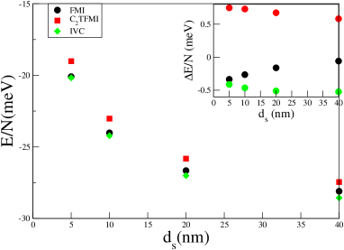
Figure 6: Main plot: Total energy per particle for ferromagnetic insulator (FMI), flavor polarized $C_{2}\mathcal{T}$ breaking insulator ($C_{2}\mathcal{T}$FMI) and intervalley coherent (IVC) states at half filling for various values of the gate distance $d_{s}$. Inset: the relative energy $\Delta E$ to the average energy of these three states to clarify the small energy difference.

References

- Cao et al. (2018a) Y. Cao, V. Fatemi, S. Fang, K. Watanabe, T. Taniguchi, E. Kaxiras, and P. Jarillo-Herrero, Nature 556, 43 (2018a).
- Cao et al. (2018b) Y. Cao, V. Fatemi, A. Demir, S. Fang, S. L. Tomarken, J. Y. Luo, J. D. Sanchez-Yamagishi, K. Watanabe, T. Taniguchi, E. Kaxiras, R. C. Ashoori, and P. Jarillo-Herrero, Nature 556, 80 (2018b).
- Rozhkov et al. (2016) A. Rozhkov, A. Sboychakov, A. Rakhmanov, and F. Nori, Physics Reports 648, 1 (2016), electronic properties of graphene-based bilayer systems.
- Lee et al. (2006) P. A. Lee, N. Nagaosa, and X.-G. Wen, Rev. Mod. Phys. 78, 17 (2006).
- Sharpe et al. (2019) A. L. Sharpe, E. J. Fox, A. W. Barnard, J. Finney, K. Watanabe, T. Taniguchi, M. A. Kastner, and D. Goldhaber-Gordon, Science 365, 605 (2019).
- Serlin et al. (2019) M. Serlin, C. L. Tschirhart, H. Polshyn, Y. Zhang, J. Zhu, K. Watanabe, T. Taniguchi, L. Balents, and A. F. Young, Science (2019), 10.1126/science.aay5533.
- Lu et al. (2019) X. Lu, P. Stepanov, W. Yang, M. Xie, M. A. Aamir, I. Das, C. Urgell, K. Watanabe, T. Taniguchi, G. Zhang, A. Bachtold, A. H. MacDonald, and D. K. Efetov, Nature 574, 653 (2019).
- Jiang et al. (2019) Y. Jiang, X. Lai, K. Watanabe, T. Taniguchi, K. Haule, J. Mao, and E. Y. Andrei, Nature 573, 91 (2019).
- Kerelsky et al. (2019) A. Kerelsky, L. J. McGilly, D. M. Kennes, L. Xian, M. Yankowitz, S. Chen, K. Watanabe, T. Taniguchi, J. Hone, C. Dean, A. Rubio, and A. N. Pasupathy, Nature 572, 95 (2019).
- Xie et al. (2019) Y. Xie, B. Lian, B. Jäck, X. Liu, C.-L. Chiu, K. Watanabe, T. Taniguchi, B. A. Bernevig, and A. Yazdani, Nature 572, 101 (2019).
- Choi et al. (2019) Y. Choi, J. Kemmer, Y. Peng, A. Thomson, H. Arora, R. Polski, Y. Zhang, H. Ren, J. Alicea, G. Refael, F. von Oppen, K. Watanabe, T. Taniguchi, and S. Nadj-Perge, Nature Physics 15, 1174 (2019).
- Yankowitz et al. (2019) M. Yankowitz, S. Chen, H. Polshyn, Y. Zhang, K. Watanabe, T. Taniguchi, D. Graf, A. F. Young, and C. R. Dean, Science 363, 1059 (2019).
- Po et al. (2018a) H. C. Po, L. Zou, A. Vishwanath, and T. Senthil, Phys. Rev. X 8, 031089 (2018a).
- Isobe et al. (2018) H. Isobe, N. F. Q. Yuan, and L. Fu, Phys. Rev. X 8, 041041 (2018).
- Liu et al. (2018) C.-C. Liu, L.-D. Zhang, W.-Q. Chen, and F. Yang, Phys. Rev. Lett. 121, 217001 (2018).
- Xu and Balents (2018) C. Xu and L. Balents, Phys. Rev. Lett. 121, 087001 (2018).
- Wu et al. (2018) F. Wu, A. H. MacDonald, and I. Martin, Phys. Rev. Lett. 121, 257001 (2018).
- Lian et al. (2019) B. Lian, Z. Wang, and B. A. Bernevig, Phys. Rev. Lett. 122, 257002 (2019).
- Huang et al. (2019) T. Huang, L. Zhang, and T. Ma, Science Bulletin 64, 310 (2019).
- Kozii et al. (2019) V. Kozii, H. Isobe, J. W. F. Venderbos, and L. Fu, Phys. Rev. B 99, 144507 (2019).
- Wu (2019) F. Wu, Phys. Rev. B 99, 195114 (2019).
- Roy and Juričić (2019) B. Roy and V. Juričić, Phys. Rev. B 99, 121407 (2019).
- Tang et al. (2019) Q.-K. Tang, L. Yang, D. Wang, F.-C. Zhang, and Q.-H. Wang, Phys. Rev. B 99, 094521 (2019).
- Kang and Vafek (2019) J. Kang and O. Vafek, Phys. Rev. Lett. 122, 246401 (2019).
- Zhang et al. (2019) Y.-H. Zhang, D. Mao, and T. Senthil, Phys. Rev. Research 1, 033126 (2019).
- Sboychakov et al. (2019) A. O. Sboychakov, A. V. Rozhkov, A. L. Rakhmanov, and F. Nori, Phys. Rev. B 100, 045111 (2019).
- Xu et al. (2018) X. Y. Xu, K. T. Law, and P. A. Lee, Phys. Rev. B 98, 121406 (2018).
- Xie and MacDonald (2020) M. Xie and A. H. MacDonald, Phys. Rev. Lett. 124, 097601 (2020).
- Liu and Dai (2019) J. Liu and X. Dai, “Spontaneous symmetry breaking and topology in twisted bilayer graphene: the nature of the correlated insulating states and the quantum anomalous hall effect,” (2019), arXiv:1911.03760 [cond-mat.str-el] .
- Liu et al. (2019) S. Liu, E. Khalaf, J. Y. Lee, and A. Vishwanath, “Nematic topological semimetal and insulator in magic angle bilayer graphene at charge neutrality,” (2019), arXiv:1905.07409 [cond-mat.str-el] .
- Bultinck et al. (2019) N. Bultinck, E. Khalaf, S. Liu, S. Chatterjee, A. Vishwanath, and M. P. Zaletel, “Ground state and hidden symmetry of magic angle graphene at even integer filling,” (2019), arXiv:1911.02045 [cond-mat.str-el] .
- Rademaker et al. (2019) L. Rademaker, D. A. Abanin, and P. Mellado, Phys. Rev. B 100, 205114 (2019).
- Wu and Das Sarma (2020) F. Wu and S. Das Sarma, Phys. Rev. Lett. 124, 046403 (2020).
- Guinea and Walet (2018) F. Guinea and N. R. Walet, Proceedings of the National Academy of Sciences 115, 13174 (2018), https://www.pnas.org/content/115/52/13174.full.pdf .
- Seo et al. (2019) K. Seo, V. N. Kotov, and B. Uchoa, Phys. Rev. Lett. 122, 246402 (2019).
- Bistritzer and MacDonald (2011) R. Bistritzer and A. H. MacDonald, Proceedings of the National Academy of Sciences 108, 12233 (2011), https://www.pnas.org/content/108/30/12233.full.pdf .
- Lopes dos Santos et al. (2012) J. M. B. Lopes dos Santos, N. M. R. Peres, and A. H. Castro Neto, Phys. Rev. B 86, 155449 (2012).
- Yuan and Fu (2018) N. F. Q. Yuan and L. Fu, Phys. Rev. B 98, 045103 (2018).
- Kang and Vafek (2018) J. Kang and O. Vafek, Phys. Rev. X 8, 031088 (2018).
- Koshino et al. (2018) M. Koshino, N. F. Q. Yuan, T. Koretsune, M. Ochi, K. Kuroki, and L. Fu, Phys. Rev. X 8, 031087 (2018).
- Po et al. (2019) H. C. Po, L. Zou, T. Senthil, and A. Vishwanath, Phys. Rev. B 99, 195455 (2019).
- Carr et al. (2019) S. Carr, S. Fang, H. C. Po, A. Vishwanath, and E. Kaxiras, Phys. Rev. Research 1, 033072 (2019).
- Haldane (1983) F. D. M. Haldane, Phys. Rev. Lett. 51, 605 (1983).
- Tarnopolsky et al. (2019) G. Tarnopolsky, A. J. Kruchkov, and A. Vishwanath, Phys. Rev. Lett. 122, 106405 (2019).
- Nam and Koshino (2017) N. N. T. Nam and M. Koshino, Phys. Rev. B 96, 075311 (2017).
- Po et al. (2018b) H. C. Po, H. Watanabe, and A. Vishwanath, Phys. Rev. Lett. 121, 126402 (2018b).
- Ahn et al. (2019) J. Ahn, S. Park, and B.-J. Yang, Phys. Rev. X 9, 021013 (2019).