Squeezing of primordial gravitational waves as quantum discord

Abstract

We investigate the squeezing of primordial gravitational waves (PGWs) in terms of quantum discord. We construct a classical state of PGWs without quantum discord and compare it with the Bunch-Davies vacuum. Then it is shown that the oscillatory behavior of the angular-power spectrum of the cosmic microwave background (CMB) fluctuations induced by PGWs can be the signature of the quantum discord of PGWs. In addition, we discuss the effect of quantum decoherence on the entanglement and the quantum discord of PGWs for super-horizon modes. For the state of PGWs with decoherence effect, we examine the decoherence condition and the correlation condition introduced by C. Kiefer et al. (Class. Quantum Grav. 24 (2007) 1699). We show that the decoherence condition is not sufficient for the separability of PGWs and the correlation condition implies that the PGWs in the matter-dominated era have quantum discord.

I Introduction

In modern cosmology, the early stage of the universe is described by inflation models. The theory of inflation predicts primordial quantum fluctuations as the origin of the structure of our universe and primordial gravitational waves (PGWs). PGWs can be the evidence of inflation, and its quantum feature is expected to give the information of quantum gravity. It is predicted that PGWs generated in the inflation era have the squeezed distribution Grischuk1989 ; Grischuk1990 . If their statistical feature is observed then it can support inflation. The detection of the squeezing effect of PGWs by ground- and space-based gravitational interferometers was discussed by B. Allen, E. E. Flanagan and M. A. Papa Allen2000 . According to their analysis, the detector with a very narrow band is required to detect the squeezing effect. The estimated bandwidth is around the present Hubble parameter, and it is difficult to detect the squeezed property of PGWs practically. On the other hand, S. Bose and L. P. Grishchuk Bose2002 considered the indirect observations of squeezing feature of PGWs by CMB fluctuations. They showed that the squeezing effect appears as the oscillatory behavior of the angular-power spectrum of the CMB temperature fluctuations induced by PGWs. This oscillation caused by PGWs is different from the baryon acoustic oscillation induced mainly by primordial density fluctuations. The contribution of PGWs to the acoustic oscillation is very small.

In order to characterize quantum feature of primordial fluctuations, the notion of quantum correlations is often applied. In particular, quantum entanglement of primordial fluctuations in the cosmological background has been investigated Nambu2008 ; Nambu2011 ; Maldacena2012 ; Kanno2014 ; Kanno2015 ; Matsumura2018 . In previous works Maldacena2012 ; Matsumura2018 , it was shown that the entanglement of primordial fluctuations remains during inflation. Although quantum entanglement is adopted to characterize the nonlocal properties of quantum mechanics, it describes only a part of quantum correlations. Quantum discord is a kind of quantum correlations Oliver2001 ; Henderson2001 and is robust against quantum decoherence. In the cosmological context, quantum discord was investigated in several works Nambu2011 ; Lim2015 ; Martin2016 ; Kanno2016 ; Hollowood2017 .

In this paper, we examine the squeezed nature of PGWs in terms of quantum correlations. In the field of quantum information, it is known that the squeezing of states is related to quantum correlations. The oscillatory behavior of PGWs originated from the squeezing can be the evidence of quantum correlation. In order to clarify the relation between the oscillatory behavior and quantum correlations, we introduce a classical state of PGWs under several assumptions. The meaning of classicality is defined based on the absence of quantum discord. The constructed classical state tells us that the oscillatory feature of PGWs is associated with quantum discord. We compute the angular-power spectrum of the CMB temperature fluctuations caused by PGWs and find that there is no oscillatory behaviors for the classical state of PGWs unlike the Bunch-Davies vacuum. Our analysis provides the meaning of the oscillatory behavior in terms of quantum correlations. We can regard it as the signature of quantum discord of PGWs.

Furthermore we investigate how the quantum correlation of PGWs is affected by the quantum decoherence for super-horizon modes. Under the assumption that sub-horizon modes of PGWs does not decohere, the decoherence condition and the correlation condition are computed. The decoherence condition implies the loss of coherence of the Bunch-Davies vacuum, and the correlation condition means the sufficient squeezing of the Wigner function for a considering mode in the phase space. Through the calculation, we show that the decoherence condition for the super-horizon modes does not mean the separability of the decohered state of PGWs. We further find that the correlation condition leads to the survival of the quantum discord of PGWs in the matter-dominated era.

This paper is organized as follows. In Sec. II, we review the linear theory of a tensor perturbation of the Friedmann-Lemaitre-Robertson-Walker (FLRW) metric and the oscillatory feature of the correlation function of the tensor field. In Sec. III, we construct a classical state of PGWs and clarify the connection between the oscillatory behavior of the angular-power spectrum and the quantum discord of PGWs. In Sec. IV, we evaluate the decoherence and the correlation conditions for the decohered state of PGWs and discuss the relation to the quantum correlations of PGWs in the matter era. The section V is devoted to summary. We use the natural unit $\hbar=c=1$ through this paper.

II Quantum tensor perturbation in inflation, radiation and matter era

In this section, we demonstrate the oscillatory behavior of the correlation function of PGWs. We consider a tensor perturbation of the spatially flat FLRW metric. The perturbed metric of the spacetime is

$$ds^{2}=a^{2}(\eta)[-d\eta^{2}+(\delta_{ij}+h_{ij})dx^{i}dx^{j}],$$ (1)

where $\eta$ is the conformal time and $h_{ij}$ represents the tensor perturbation with $\partial^{j}h_{ij}=\delta^{ij}h_{ij}=0$ ($i,j=1,2,3$). We assume that the universe has instantaneous transitions at $\eta=\eta_{\text{r}}$ and $\eta=\eta_{\text{m}}$ for its expansion law. The scale factor $a$ is given as

$$a(\eta)=\begin{cases}-\dfrac{1}{H_{\text{inf}}\,(\eta-2\eta_{\text{r}})}&(-\infty<\eta\leq\eta_{\text{r}})\\ \dfrac{\eta}{H_{\text{inf}}\,\eta^{2}_{\text{r}}}&(\eta_{\text{r}}<\eta\leq\eta_{\text{m}})\\ \dfrac{1}{4}\left(1+\dfrac{\eta}{\eta_{\text{m}}}\right)^{2}\dfrac{\eta_{\text{m}}}{H_{\text{inf}}\,\eta_{\text{r}}^{2}}&(\eta_{\text{m}}<\eta)\end{cases}.$$ (2)

Each form of the scale factor represents the expansion law in the inflation, radiation and matter era. The inflationary universe is assumed to be the de Sitter spacetime with the Hubble parameter $H_{\text{inf}}$. The perturbed Einstein-Hilbert action up to the second order of $h_{ij}$ is

$$S=\frac{M^{2}_{\text{pl}}}{2}\int d^{4}x\sqrt{-g}R\approx\frac{M^{2}_{\text{pl}}}{8}\int d\eta\,d^{3}x\,a^{2}\left(h^{ij}{}^{\prime}h^{\prime}_{ij}-\partial^{k}h^{ij}\partial_{k}h_{ij}\right),$$ (3)

where prime denotes the derivative of the conformal time $\eta$ and $M_{\text{pl}}$ is the reduced Planck mass $1/\sqrt{8\pi G}$. In the following, we use the rescaled perturbation and its conjugate momentum

$$y_{ij}:=ah_{ij},\quad\pi_{ij}:=y^{\prime}_{ij}-\frac{a^{\prime}}{a}y_{ij}.$$ (4)

Since the background spacetime is invariant under spatial rotations and translations, the tensor perturbation can be decomposed as

$$y_{ij}(\bm{x},\eta) =\frac{\sqrt{2}}{M_{\text{pl}}}\int\frac{d^{3}q}{(2\pi)^{3/2}}\sum_{\lambda}y_{\lambda}(\bm{q},\eta)e_{ij}(\hat{q},\lambda)e^{i\bm{q}\cdot\bm{x}},$$ (5)

$$\pi_{ij}(\bm{x},\eta) =\frac{M_{\text{pl}}}{\sqrt{2}}\int\frac{d^{3}q}{(2\pi)^{3/2}}\sum_{\lambda}\pi_{\lambda}(\bm{q},\eta)e_{ij}(\hat{q},\lambda)e^{i\bm{q}\cdot\bm{x}},$$ (6)

where $\lambda=1,2$ denote the labels of the polarization and the polarization tensor $e_{ij}(\hat{q},\lambda)$ with $\hat{q}=\bm{q}/|\bm{q}|$ is chosen as

$$\hat{q}^{i}e_{ij}(\hat{q},\lambda)=e^{i}{}_{i}(\hat{q},\lambda)=0,$$ (7)

$$e^{ij*}(\hat{q},\lambda)e_{ij}(\hat{q},\lambda^{\prime})=2\delta_{\lambda\lambda^{\prime}},$$ (8)

$$e_{ij}^{*}(\hat{q},\lambda)=e_{ij}(-\hat{q},\lambda).$$ (9)

Eq. (7) corresponds to the traceless and transverse conditions and Eq. (8) is the normalization condition. The representation of the parity transformation for the polarization tensor is fixed by Eq. (9). The reality condition of the tensor perturbation with (9) implies that the variables $y_{\lambda}$ and $\pi_{\lambda}$ satisfy

$$y^{*}_{\lambda}(\bm{q},\eta)=y_{\lambda}(-\bm{q},\eta),\quad\pi^{*}_{\lambda}(\bm{q},\eta)=\pi_{\lambda}(-\bm{q},\eta).$$ (10)

From the perturbed action (3), the mode equation is

$$y^{\prime\prime}_{\lambda}(\bm{q},\eta)+\Bigl{(}q^{2}-\frac{a^{\prime\prime}}{a}\Bigr{)}y_{\lambda}(\bm{q},\eta)=0,$$ (11)

where $q=|\bm{q}|$. To quantize the tensor perturbation, we impose the canonical commutation relations

$$[\hat{y}_{\lambda}(\bm{q},\eta),\hat{y}_{\lambda^{\prime}}(\bm{q}^{\prime},\eta)]=[\hat{\pi}_{\lambda}(\bm{q},\eta),\hat{\pi}_{\lambda^{\prime}}(\bm{q}^{\prime},\eta)]=0,$$ (12)

$$[\hat{y}_{\lambda}(\bm{q},\eta),\hat{\pi}_{\lambda^{\prime}}(\bm{q}^{\prime},\eta)]=i\delta_{\lambda\lambda^{\prime}}\delta^{3}(\bm{q}+\bm{q}^{\prime}).$$ (13)

We denote the solution of the equation of motion (11) as $f_{q}$ and define the function $g_{q}=i(f^{\prime}_{q}-a^{\prime}f_{q}/a)$. We fix the normalization of the mode function as

$$f_{q}(\eta)g^{*}_{q}(\eta)+f^{*}_{q}(\eta)g_{q}(\eta)=1,$$ (14)

and expand the canonical variables $\hat{y}_{\lambda}$ and $\hat{\pi}_{\lambda}$ as follows:

$$\hat{y}_{\lambda}(\bm{q},\eta) =f_{q}(\eta)\hat{a}_{\lambda}(\bm{q})+f^{*}_{q}(\eta)\hat{a}^{\dagger}_{\lambda}(-\bm{q}),$$ (15)

$$\hat{\pi}_{\lambda}(\bm{q},\eta) =(-i)\left(g_{q}(\eta)\hat{a}_{\lambda}(\bm{q})-g^{*}_{q}(\eta)\hat{a}^{\dagger}_{\lambda}(-\bm{q})\right),$$ (16)

where $\hat{a}_{\lambda}$ is the annihilation operator satisfying

$$[\hat{a}_{\lambda}(\bm{q}),\hat{a}_{\lambda^{\prime}}(\bm{q}^{\prime})]=0,$$ (17)

$$[\hat{a}_{\lambda}(\bm{q}),\hat{a}^{\dagger}_{\lambda^{\prime}}(\bm{q}^{\prime})]=\delta_{\lambda\lambda^{\prime}}\delta^{3}(\bm{q}-\bm{q}^{\prime}).$$ (18)

The equation of the mode function is solved for each epoch, and junction conditions at $\eta=\eta_{\text{r}}$ and $\eta=\eta_{\text{m}}$ yield the full solution of the tensor perturbation in the FLRW universe. We adopt the following mode function for the inflation era

$$u^{\text{inf}}_{q}(\eta)=\frac{1}{\sqrt{2q}}\left(1-\frac{i}{q(\eta-2\eta_{\text{r}})}\right)e^{-iq(\eta-2\eta_{\text{r}})},$$ (19)

and assume that the initial quantum state of PGWs is the Bunch-Davies vacuum $\ket{0^{\text{BD}}}$ defined by

$$\hat{a}_{\lambda}(\bm{q})\ket{0^{\text{BD}}}=0.$$ (20)

With the junction conditions, we find the full solution of the mode function as

$$f_{q}(\eta)=\begin{cases}u^{\text{inf}}_{q}(\eta)&(-\infty<\eta\leq\eta_{\text{r}})\\ \alpha_{q}u^{\text{rad}}_{q}(\eta)+\beta_{q}u^{\text{rad}*}_{q}(\eta)&(\eta_{\text{r}}<\eta\leq\eta_{\text{m}})\\ \gamma_{q}u^{\text{mat}}_{q}(\eta)+\delta_{q}u^{\text{mat}*}_{q}(\eta)&(\eta_{\text{m}}<\eta)\end{cases},$$ (21)

where $u^{\text{rad}}_{q}$ and $u^{\text{mat}}_{q}$ are the positive frequency mode solutions in the radiation- and matter-dominated era and the coefficients $\alpha_{q},\beta_{q},\gamma_{q}$ and $\delta_{q}$ are fixed by the junction conditions. In particular, the mode function $u^{\text{rad}}_{q}$ is given as

$$u^{\text{rad}}_{q}(\eta)=\frac{1}{\sqrt{2q}}\,e^{-iq\eta}.$$ (22)

From the solution $f_{q}$, the function $g_{q}$ is obtained as

$$g_{q}(\eta)=\begin{cases}v^{\text{inf}}_{q}(\eta)&(-\infty<\eta\leq\eta_{\text{r}})\\ \alpha_{q}v^{\text{rad}}_{q}(\eta)-\beta_{q}v^{\text{rad}*}_{q}(\eta)&(\eta_{\text{r}}<\eta\leq\eta_{\text{m}})\\ \gamma_{q}v^{\text{mat}}_{q}(\eta)-\delta_{q}v^{\text{mat}*}_{q}(\eta)&(\eta_{\text{m}}<\eta)\end{cases},$$ (23)

where the functions $v^{\text{inf}}_{q},v^{\text{rad}}_{q}$ and $v^{\text{mat}}_{q}$ are given by the definition of the function $g_{q}(\eta)$. The explicit formulas of $v^{\text{inf}}_{q}$ and $v^{\text{rad}}_{q}$ are

$$v^{\text{inf}}_{q}(\eta) =\sqrt{\frac{q}{2}}\,e^{-iq\eta},$$ (24)

$$v^{\text{rad}}_{q}(\eta) =\sqrt{\frac{q}{2}}\,\Bigl{(}1-\frac{i}{q\eta}\Bigr{)}e^{-iq\eta}.$$ (25)

The normalizations of $u^{\text{inf}}_{q},v^{\text{inf}}_{q},u^{\text{rad}}_{q}$, and $v^{\text{rad}}_{q}$ are chosen so that Eq. (14) is satisfied for each pair $(u^{\text{inf}}_{q},v^{\text{inf}}_{q})$ and $(u^{\text{rad}}_{q},v^{\text{rad}}_{q})$. The Bogolyubov coefficients $\alpha_{q},\beta_{q},\gamma_{q}$ and $\delta_{q}$ satisfy the normalization conditions

$$|\alpha_{q}|^{2}-|\beta_{q}|^{2}=1,\quad|\gamma_{q}|^{2}-|\delta_{q}|^{2}=1.$$ (26)

The coefficients $\alpha_{q}$ and $\beta_{q}$ are determined by the junction conditions at $\eta=\eta_{\text{r}}$:

$$\alpha_{q}=\Bigl{(}1+\frac{i}{q\eta_{\text{r}}}-\frac{1}{2q^{2}\eta_{\text{r}}^{2}}\Bigr{)}e^{2iq\eta_{\text{r}}},\quad\beta_{q}=\frac{1}{2q^{2}\eta_{\text{r}}^{2}}.$$ (27)

The explicit formulas of the functions $u^{\text{mat}}_{q},v^{\text{mat}}_{q}$ and the coefficients $\gamma_{q},\delta_{q}$ are not needed in the following analysis. This is because we are interested in the super-horizon mode at the end of inflation and the sub-horizon mode at the radiation-matter equality time, that is,

$$q\eta_{\text{r}}\ll 1,\quad q\eta_{\text{m}}\gg 1.$$ (28)

The sub-horizon condition $q\eta_{\text{m}}\gg 1$ implies that the solution $f_{q}$ in the matter era can be approximated by that for the radiation era.

Let us demonstrate the oscillatory behavior of the correlation function of PGWs. In order to make a clear connection between the oscillatory behavior and quantum correlations, we introduce

$$\hat{A}_{\lambda}(\bm{q},\eta)=\sqrt{\frac{q}{2}}\,\hat{y}_{\lambda}(\bm{q},\eta)+\frac{i}{\sqrt{2q}}\hat{\pi}_{\lambda}(\bm{q},\eta).$$ (29)

The operator $\hat{A}_{\lambda}$ for a sub-horizon mode is equivalent to the annihilation operator defined by the positive frequency mode in each era. In fact, in the radiation or the matter era $\eta_{\text{r}}<\eta$, the operator $\hat{A}_{\lambda}$ for the sub-horizon mode $q\eta\gg 1$ is approximated as

$$\hat{A}_{\lambda}(\bm{q},\eta)\sim\hat{b}_{\lambda}(\bm{q})e^{-iq\eta},$$ (30)

where $\hat{b}_{\lambda}$ is given by

$$\hat{b}_{\lambda}(\bm{q})=\alpha_{q}\hat{a}_{\lambda}(\bm{q})+\beta^{*}_{q}\hat{a}^{\dagger}_{\lambda}(-\bm{q}).$$ (31)

The operator $\hat{b}_{\lambda}$ are the annihilation operator defined by the positive frequency mode $u^{\text{rad}}_{q}$ after inflation ($u^{\text{rad}}_{q}$ is also the positive frequency mode in the matter era for $q\eta_{\text{m}}\gg 1$). Hence the operator $\hat{A}_{\lambda}$ for the sub-horizon mode has the same role as $\hat{b}_{\lambda}$. The correlation function for the field amplitude $\hat{y}_{\lambda}$ is

$$\bra{0^{\text{BD}}}\hat{y}_{\lambda}(\bm{q},\eta)\hat{y}_{\lambda^{\prime}}(\bm{q}^{\prime},\eta)\ket{0^{\text{BD}}}=\frac{1}{2q}\left(2n_{q}(\eta)+1+c_{q}(\eta)+c^{*}_{q}(\eta)\right)\delta_{\lambda\lambda^{\prime}}\delta^{3}(\bm{q}+\bm{q}^{\prime}),$$ (32)

where we used $\hat{y}_{\lambda}(\bm{q},\eta)=(\hat{A}_{\lambda}(\bm{q},\eta)+\hat{A}^{\dagger}_{\lambda}(-\bm{q},\eta))/\sqrt{2q}$ and introduced $n_{q}$ and $c_{q}$ by

$$\bra{0^{\text{BD}}}\hat{A}^{\dagger}_{\lambda}(\bm{q},\eta)\hat{A}_{\lambda^{\prime}}(\bm{q}^{\prime},\eta)\ket{0^{\text{BD}}} =n_{q}(\eta)\delta_{\lambda\lambda^{\prime}}\delta^{3}(\bm{q}-\bm{q}^{\prime}),$$ (33)

$$\bra{0^{\text{BD}}}\hat{A}_{\lambda}(\bm{q},\eta)\hat{A}_{\lambda^{\prime}}(\bm{q}^{\prime},\eta)\ket{0^{\text{BD}}} =c_{q}(\eta)\delta_{\lambda\lambda^{\prime}}\delta^{3}(\bm{q}+\bm{q}^{\prime}).$$ (34)

The function $n_{q}$ represents the mean particle number and $c_{q}$ characterizes the quantum coherence of the Bunch-Davies vacuum. The functions $n_{q}$ and $c_{q}$ completely determine the quantum property of the Bunch-Davies vacuum. We evaluate the correlation function in the matter era. For the target range of the wave number $1/\eta_{\text{m}}\ll q\ll 1/\eta_{\text{r}}$ (28), the functions $n_{q}$ and $c_{q}$ for the sub-horizon mode $q\eta\gg 1$ are computed as

$$n_{q}(\eta) \sim|\beta_{q}|^{2},$$ (35)

$$c_{q}(\eta) \sim\alpha_{q}\beta^{*}_{q}e^{-2iq\eta}\sim-|\beta_{q}|^{2}e^{-2iq\eta},$$ (36)

where the second approximation in Eq. (36) follows from $q\eta_{\text{r}}\ll 1$. The behavior of the correlation function of $\hat{y}_{\lambda}$ in the matter-dominated era is obtained as

$$\bra{0^{\text{BD}}}\hat{y}_{\lambda}(\bm{q},\eta)\hat{y}_{\lambda^{\prime}}(\bm{q}^{\prime},\eta)\ket{0^{\text{BD}}}\sim\frac{|\beta_{q}|^{2}}{q}(1-\cos(2q\eta))\delta_{\lambda\lambda^{\prime}}\delta^{3}(\bm{q}+\bm{q}^{\prime}),$$ (37)

where the cosine term comes from $c_{q}(\eta)$, and the correlation function oscillates in time. In terms of the Fock space defined by $\hat{A}_{\lambda}$, the Bunch-Davies vacuum can be expressed as

$$\ket{0^{\text{BD}}} \propto\bigotimes_{\bm{q}\in\mathbb{R}^{3+}}\bigotimes_{\lambda}\exp\left[\frac{c_{q}}{n_{q}+1}\hat{A}^{\dagger}_{\lambda}(\bm{q},\eta)\hat{A}^{\dagger}_{\lambda}(-\bm{q},\eta)\right]\ket{0;\eta}$$

$$=\bigotimes_{\bm{q}\in\mathbb{R}^{3+}}\bigotimes_{\lambda}\sum^{\infty}_{n=0}\left(\frac{c_{q}}{n_{q}+1}\right)^{n}\ket{n_{\bm{q},\lambda}\,n_{-\bm{q},\lambda};\eta},$$ (38)

where the state $\ket{0;\eta}$ is defined by $\hat{A}_{\lambda}(\bm{q},\eta)\ket{0;\eta}=0$ and $\mathbb{R}^{3+}:=\{(x,y,z)|(x,y,z)\in\mathbb{R}^{3},z\geq 0\}$. The function $c_{q}$, which characterizes the coherence between the modes $\bm{q}$ and $-\bm{q}$, leads to the squeezing and rotation of the Wigner function in the phase space. From Eq. (20), the wave function of the Bunch-Davies vacuum for a single mode $\bm{q}$ and a polarization $\lambda$ is

$$\psi^{\text{BD}}(y,\eta)=\sqrt{\frac{2\Omega_{q}^{\text{R}}}{\pi}}\exp(-\Omega_{q}(\eta)|y|^{2}),\quad\Omega_{q}(\eta)=\frac{g^{*}_{q}(\eta)}{f^{*}_{q}(\eta)},$$ (39)

where we omitted the labels $\bm{q}$ and $\lambda$, and the superscript R denotes the real part. The Wigner function $W^{\text{BD}}(y,\pi_{y},\eta)$ of the density matrix $\rho^{\text{BD}}(y,y^{\prime},\eta)=\psi^{\text{BD}}(y,\eta)[\psi^{\text{BD}}(y^{\prime},\eta)]^{*}$ is given by

$$W^{\text{BD}}(y,\pi_{y},\eta) =\frac{1}{(2\pi)^{2}}\int dx^{\text{R}}dx^{\text{I}}\,e^{i(\pi^{\text{R}}_{y}x^{\text{R}}+\pi^{\text{I}}_{y}x^{\text{I}})}\rho^{\text{BD}}(y-x/2,y+x/2,\eta)$$

$$=w^{\text{BD}}(y^{\text{R}},\pi^{\text{R}}_{y},\eta)w^{\text{BD}}(y^{\text{I}},\pi^{\text{I}}_{y},\eta),$$ (40)

$$w^{\text{BD}}(x,p,\eta) =\frac{1}{\pi}\exp\left[-2\Omega_{q}^{\text{R}}\,x^{2}-\frac{2}{\Omega^{\text{R}}_{q}}\left(p+\Omega_{q}^{\text{I}}\,x\right)^{2}\right],$$ (41)

where the superscript I denotes the imaginary part. Fig. 1 schematically represents the behavior of the Wigner function $w^{\text{BD}}(y^{\text{R}},\pi^{\text{R}}_{y},\eta)$.

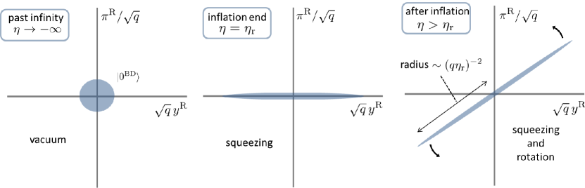
Figure 1: The behavior of the Wigner ellipse of the Bunch-Davis vacuum in the phase space $(\sqrt{q}\,y^{\text{R}},\pi^{\text{R}}/\sqrt{q})$. Left panel: the initial vacuum at the past infinity. Middle panel: the squeezed Wigner ellipse at the end of inflation. Right panel: the squeezed and rotated ellipse after the inflation.

In Fig. 1, the left panel represents the initial vacuum state at the past infinity $\eta\rightarrow-\infty$ and the middle panel represents the squeezed vacuum by the inflationary expansion. The right panel shows the Wigner ellipse after the end of inflation for a sub-horizon mode. The Wigner function is further squeezed until the horizon re-entry. After that, the Wigner ellipse rotates during the radiation and matter era. (Its thickness is around $\hbar=1$ in the right panel of Fig. 1, however it can be ignored in (37).) The oscillation of the correlation function corresponds to the rotation of the Wigner ellipse in the phase space.

In order to understand the oscillatory feature from the viewpoint of quantum superpositions, we have introduced the two modes $\bm{q}$ and $-\bm{q}$ by defining the annihilation operator (29). On the other hand, we have used the Wigner function of the single mode $\bm{q}$ for the real (or imaginary) part of the field $\hat{y}_{\lambda}$ to explain the squeezing feature of the state. These two treatments are connected by the following relation

$$\hat{y}^{\text{R}}_{\lambda}(\bm{q},\eta)=\frac{1}{2\sqrt{2q}}\left(\hat{A}_{\lambda}(\bm{q},\eta)+\hat{A}^{\dagger}_{\lambda}(-\bm{q},\eta)+\hat{A}^{\dagger}_{\lambda}(\bm{q},\eta)+\hat{A}_{\lambda}(-\bm{q},\eta)\right),$$ (42)

where $\bm{q}\in\mathbb{R}^{3+}$ because of the relation $\hat{y}^{\text{R}}_{\lambda}(-\bm{q},\eta)=\hat{y}^{\text{R}}_{\lambda}(\bm{q},\eta)$. The correlation function of $y^{\text{R}}_{\lambda}$ is

$$\bra{0^{\text{BD}}}\hat{y}^{\text{R}}_{\lambda}(\bm{q},\eta)\hat{y}^{\text{R}}_{\lambda^{\prime}}(\bm{q}^{\prime},\eta)\ket{0^{\text{BD}}}=\frac{1}{4q}\left(2n_{q}(\eta)+1+c_{q}(\eta)+c^{*}_{q}(\eta)\right)\delta_{\lambda\lambda^{\prime}}\delta^{3}(\bm{q}-\bm{q}^{\prime}),$$ (43)

and contains the function $c_{q}(\eta)$ characterizing the quantum coherence for the modes $\bm{q}$ and $-\bm{q}$.

III Relation between the oscillatory behavior and quantum discord

In this section we clarify the relation between the oscillatory behavior of the CMB angular-power spectrum caused by PGWs and quantum discord. For this purpose, we introduce the notion of the classically correlated state. A given bipartite state $\rho_{\text{AB}}$ is called classically correlated Oliver2001 ; Oppenheim2002 if the state has the following form

$$\rho_{\text{AB}}=\sum_{i,j}p_{ij}\ket{\psi^{i}_{\text{A}}}\bra{\psi^{i}_{\text{A}}}\otimes\ket{\phi^{j}_{\text{B}}}\bra{\phi^{j}_{\text{B}}},$$ (44)

where $p_{ij}$ is a joint probability ($p_{ij}\geq 0,~{}\sum_{i,j}p_{ij}=1$) and characterizes the classical correlation between A and B. The vectors $\ket{\psi^{i}_{\text{A}}}$ and $\ket{\phi^{k}_{\text{B}}}$ of each system A and B satisfy the orthonormal conditions

$$\langle\psi^{i}_{\text{A}}|\psi^{j}_{\text{A}}\rangle=\delta^{ij},\quad\langle\phi^{k}_{\text{B}}|\phi^{l}_{\text{B}}\rangle=\delta^{kl}.$$ (45)

The particular feature of classically correlated states is that there is a rank-1 projective measurement for the subsystem A or B such that the states are not disturbed Oliver2001 in the following sense:

$$\sum_{i}\hat{P}^{i}_{\text{A}}\rho_{\text{AB}}\hat{P}^{i}_{\text{A}}=\sum_{j}\hat{P}^{j}_{\text{B}}\rho_{\text{AB}}\hat{P}^{j}_{\text{B}}=\rho_{\text{AB}},$$ (46)

where $\hat{P}^{i}_{\text{A}}$ and $\hat{P}^{j}_{\text{B}}$ are rank-1 projective operators satisfying $\sum_{i}\hat{P}^{i}_{\text{A}}=\hat{\mathbb{I}}_{\text{A}}$ and $\sum_{i}\hat{P}^{i}_{\text{B}}=\hat{\mathbb{I}}_{\text{B}}$. This property is not required for separable states (non-entangled states) Werner1989 defined by

$$\rho_{\text{AB}}=\sum_{i}\lambda_{i}\rho^{i}_{\text{A}}\otimes\sigma^{i}_{\text{B}},$$ (47)

where $\lambda_{i}$ is a probability, and $\rho^{i}_{\text{A}}$ and $\sigma^{i}_{\text{B}}$ are density operators. This is because $\rho^{i}_{\text{A}}$ and $\rho^{j}_{\text{A}}$ ($i\neq j$) do not have to commute each other generally, and hence separable states can be disturbed by a projective measurement for the subsystem A. It is obvious that the classically correlated states are included in the separable states by the definitions of each state.

Next we introduce quantum discord Oliver2001 as a measure of quantum correlations. Quantum discord is the difference between the mutual information of a given bipartite state $\rho_{\text{AB}}$ and its generalization with a projective measurement. The mutual information $I_{\text{AB}}$ is

$$I_{\text{AB}}=S_{\text{A}}+S_{\text{B}}-S_{\text{AB}},$$ (48)

where $S_{\text{A}},S_{\text{B}}$ and $S_{\text{AB}}$ are the von Neumann entropy of the density operators $\rho_{\text{A}}=\text{Tr}_{\text{B}}[\rho_{\text{AB}}]$, $\rho_{\text{B}}=\text{Tr}_{\text{A}}[\rho_{\text{AB}}]$ and $\rho_{\text{AB}}$, respectively. For example, $S_{\text{A}}=S(\rho_{\text{A}})=-\text{Tr}_{\text{A}}[\rho_{\text{A}}\log\rho_{\text{A}}]$. The mutual information characterizes the total correlation of the bipartite state $\rho_{\text{AB}}$. Using the conditional entropy $S_{\text{B}|\text{A}}=S_{\text{AB}}-S_{\text{A}}$, the mutual information is rewritten as

$$I_{\text{AB}}=S_{\text{B}}-S_{\text{B}|\text{A}}.$$ (49)

This second expression leads to the notion of quantum discord. As a generalization of the conditional entropy with a projective measurement, we can consider

$$J_{\text{B}|\{\hat{P}^{j}_{\text{A}}\}}=S_{\text{B}}-\sum_{i}p_{i}S_{\text{B}|\hat{P}^{i}_{\text{A}}},$$ (50)

where $p_{i}=\text{Tr}_{\text{AB}}[\hat{P}^{i}_{\text{A}}\rho_{\text{AB}}]$ and $S_{\text{B}|\hat{P}^{i}_{\text{A}}}$ is the von Neumann entropy of the density operator given by

$$\rho^{i}_{\text{B}}=\frac{\text{Tr}_{\text{A}}[\hat{P}^{i}_{\text{A}}\rho_{\text{AB}}\hat{P}^{i}_{\text{A}}]}{p_{i}}.$$ (51)

The von Neumann entropy $\sum_{i}p_{i}S_{\text{B}|\hat{P}^{i}_{\text{A}}}$ is equivalent to the conditional entropy after the projective measurement $\hat{P}^{i}_{\text{A}}$ on the system A. Quantum discord of a bipartite state $\rho_{\text{AB}}$ is the minimum of difference between the two mutual informations:

$$\delta_{\text{B}|\text{A}}:=I_{\text{AB}}-\max_{\hat{P}^{j}_{\text{A}}}J_{\text{B}|\{\hat{P}^{j}_{\text{A}}\}},$$ (52)

where we maximize over all possible projective measurements on the system A. In general, $\delta_{\text{B}|\text{A}}$ is not the same as $\delta_{\text{A}|\text{B}}$. In Ref. Oliver2001 , it was shown that $\delta_{\text{B}|\text{A}}=0=\delta_{\text{A}|\text{B}}$ for a given bipartite state if and only if the state is classically correlated. The quantities $\delta_{\text{B}|\text{A}}$ and $\delta_{\text{A}|\text{B}}$ are good indicators of the quantumness of the correlation associated with a given state.

Now, we construct a classical model (zero quantum discord state) of PGWs. Firstly, we impose the following three assumptions on the classical model:

Assumption 1.

The mode obeys the linearized Einstein equation.

Assumption 2.

The initial state is a Gaussian state.

Assumption 3.

The initial state is invariant under spatial translations and rotations.

These assumptions are accepted in the standard treatment of the linear quantum fluctuations in the FLRW universe. We denote the classical model (state) of PGWs as $\rho^{\text{cl}}$. By the assumption 1, the evolution of the Heisenberg operators is determined and hence we only have to fix the initial condition of the state $\rho^{\text{cl}}$ to identify the classical model. From the assumptions 2 and 3, the state $\rho^{\text{cl}}$ has the following expectation values for $\hat{b}_{\lambda}$ and $\hat{b}^{\dagger}_{\lambda}$ defined by (31) :

$$\text{Tr}[\hat{b}_{\lambda}(\bm{q})\rho^{\text{cl}}]=0,$$ (53)

$$\text{Tr}[\hat{b}^{\dagger}_{\lambda}(\bm{q})\hat{b}_{\lambda^{\prime}}(\bm{q}^{\prime})\rho^{\text{cl}}]=m_{q}\,\delta_{\lambda\lambda^{\prime}}\delta^{3}(\bm{q}-\bm{q}^{\prime}),$$ (54)

$$\text{Tr}[\hat{b}_{\lambda}(\bm{q})\hat{b}_{\lambda^{\prime}}(\bm{q}^{\prime})\rho^{\text{cl}}]=d_{q}\,\delta_{\lambda\lambda^{\prime}}\delta^{3}(\bm{q}+\bm{q}^{\prime}),$$ (55)

where $m_{q}$ and $d_{q}$ are free functions characterizing the initial state. Because of the translational invariance, the expectation value of the annihilation operator $\hat{b}_{\lambda}$ with nonzero modes vanishes. From the assumption of being Gaussian state, the functions $m_{q}$ and $d_{q}$ completely determine the form of the state $\rho^{\text{cl}}$.

In order to fix the two functions $m_{q}$ and $d_{q}$, we further impose the following two assumptions:

Assumption 4.

The bipartite state with modes $\bm{q}$ and $-\bm{q}$ defined by the annihilation and creation operators $\hat{b}_{\lambda}(\bm{q})$ and $\hat{b}^{\dagger}_{\lambda}(\bm{q})$ is a classically correlated state (zero discord state).

Assumption 5.

At the present time, the classical model provides the same correlation function of PGWs as the initial Bunch-Davies vacuum.

From the assumption 2,3 and 4, we can find that the state $\rho^{\text{cl}}$ is classically correlated if and only if the function $d_{q}$ vanishes. Let us show this statement. For simplicity, we omit the index of the polarization $\lambda$ and denote the state $\rho^{\text{cl}}$ with the mode $\bm{q}$ and $-\bm{q}$ as $\rho^{\text{cl}}_{\bm{q},-\bm{q}}$. When the function $d_{q}$ vanishes, the Gaussian state $\rho_{\bm{q},-\bm{q}}$ is a product state, which corresponds to a classically correlated state with the weight $p_{ij}=p_{i}^{\text{A}}p_{j}^{\text{B}}$ in Eq. (44). Conversely, if the state $\rho^{\text{cl}}_{\bm{q},-\bm{q}}$ is classically correlated, then the state $\rho^{\text{cl}}_{\bm{q},-\bm{q}}$ is represented by a product state

$$\rho^{\text{cl}}_{\bm{q},-\bm{q}}=\rho_{\bm{q}}\otimes\sigma_{-\bm{q}},$$ (56)

where $\rho_{\bm{q}}$ and $\sigma_{-\bm{q}}$ are density operators for each mode. In general, a given classically correlated state can have correlation, but classically correlated Gaussian states are product states Giorda2010 ; Adesso2010 . The Appendix A is devoted to a simple proof of this property. Then the expectation value of $\hat{b}(\bm{q})\hat{b}(-\bm{q})$ is given by

$$\text{Tr}[\hat{b}(\bm{q})\hat{b}(-\bm{q})\,\rho^{\text{cl}}_{\bm{q},-\bm{q}}]=\text{Tr}[\hat{b}(\bm{q})\,\rho_{\bm{q}}]\times\text{Tr}[\hat{b}(-\bm{q})\,\sigma_{-\bm{q}}]=0,$$ (57)

because the one-point function of the annihilation operator $\hat{b}(\bm{q})$ vanishes by the translation invariance (53). Hence the function $d_{q}$ must vanish. As $d_{q}$ characterizes the coherence of $\rho^{\text{cl}}$ (see Eq. (55)), the following statement holds: the quantum discord exists if and only if the quantum coherence for the modes $\bm{q}$ and $-\bm{q}$ exists.

We emphasize that the condition $d_{q}=0$ for the classical state cannot be derived from the separability. To judge whether a given bipartite state $\rho_{\text{AB}}$ is entangled or not, the positive partial transposed (PPT) criterion is useful Peres1996 ; Horodecki1996 ; if a bipartite state $\rho_{\text{AB}}$ is separable then the following inequality holds

$$(\rho_{\text{AB}})^{\text{T}_{\text{B}}}\geq 0,$$ (58)

where $\text{T}_{\text{B}}$ is the transposition for the subsystem B and the inequality means that $(\rho_{\text{AB}})^{\text{T}}_{\text{B}}$ has no negative eigenvalues. For the Gaussian bipartite state $\rho^{\text{cl}}_{\bm{q},-\bm{q}}$ defined by $\hat{b}(\bm{q})$ and $\hat{b}(-\bm{q})$, it is known that the PPT criterion is the necessary and sufficient condition for the separability Simon2000 ; Giedke2001 ; Fujikawa2009 . The inequality (58) for the state $\rho^{\text{cl}}_{\bm{q},-\bm{q}}$ is given by

$$m_{q}\geq|d_{q}|.$$ (59)

The derivation of the inequality (59) is shown in the appendix B. We can admit the non-entangled model of PGWs with nonzero $d_{q}$ (non-zero discord). Such a model has the following expectation value for the sub-horizon modes ($q\eta\gg 1$),

$$\text{Tr}[\hat{A}_{\lambda}(\bm{q},\eta)\hat{A}_{\lambda^{\prime}}(\bm{q}^{\prime},\eta)\rho^{\text{cl}}]\sim d_{q}e^{-2iq\eta}\delta_{\lambda\lambda^{\prime}}\delta^{3}(q+q^{\prime}),$$ (60)

and shows the oscillatory behavior of the correlation function. Hence we cannot distinguish whether the model has quantum entanglement (between $\bm{q}$ and $-\bm{q}$ modes) by just observing the oscillatory behavior.

The function $m_{q}$ is determined by the assumption 5. Using the approximated form of the annihilation operator $\hat{A}_{\lambda}$ for the sub-horizon scale (30), we obtain the correlation function of the state $\rho^{\text{cl}}$ for $q\eta_{0}\gg 1$ as

$$\text{Tr}[\hat{y}_{\lambda}(\bm{q},\eta_{0})\hat{y}_{\lambda^{\prime}}(\bm{q}^{\prime},\eta_{0})\rho^{\text{cl}}]\sim\frac{1}{2q}(2m_{q}+1)\delta_{\lambda\lambda^{\prime}}\delta^{3}(\bm{q}+\bm{q}^{\prime}),$$ (61)

where $\eta_{0}$ is the conformal time of the present day. The assumption 5 requires that the correlation function of the variables $\hat{y}_{\lambda}$ should be equal to that given by the Bunch-Davies vacuum (37). For $q\eta_{0}\gg 1$ and $q\eta_{\text{r}}\ll 1$ the function $m_{q}$ can be fixed as

$$m_{q}=n_{q}(\eta_{0})+\frac{1}{2}\Bigl{(}c_{q}(\eta_{0})+c^{*}_{q}(\eta_{0})\Bigr{)}\sim|\beta_{q}|^{2}(1-\cos(2q\eta_{0})),$$ (62)

where we used Eq. (37) at the present time $\eta_{0}$.

Here we compare our analysis with the previous work Bose2002 . They considered squeezed and non-squeezed models of PGWs. Both of these models assume the Bunch-Davies vacuum as the initial state of PGWs. The squeezed model corresponds to PGWs treated in the previous section. The non-squeezed one is constructed by assuming the following form of the mode function in the matter-dominated era

$$f_{q}(\eta)\propto\frac{e^{-iq\eta}}{\sqrt{2q}},$$ (63)

which has only the positive frequency mode. This means that there is no particle production and any squeezing effects. In Bose2002 , the specification (63) of the mode function was called the traveling wave condition, which corresponds to the classically correlated assumption in our analysis. The amplitude of the mode (63) is determined by the same procedure as our assumption 5, which was called the fair comparison in Bose2002 . For the sub-horizon mode at the present time $q\eta_{0}\gg 1$, the amplitude was given by $m_{q}$ without the cosine term in Bose2002 . The disregard of the cosine term is valid in the calculation of the angular-power spectrum. We will explain the detail of this statement later (after Eq. (73)).

Let us compare the two models of PGWs by the angular-power spectrum of CMB temperature fluctuations. The temperature fluctuations caused by the tensor perturbation is

$$\frac{\delta\hat{T}(\hat{n})}{T_{0}}=-\frac{1}{2}\hat{n}_{i}\hat{n}_{j}\int^{\eta_{0}}_{\eta_{\text{L}}}d\eta\left[\frac{\partial}{\partial\eta}\hat{h}_{ij}\right]_{r=\eta_{0}-\eta}=-\frac{1}{2}\hat{n}_{i}\hat{n}_{j}\int^{\eta_{0}}_{\eta_{\text{L}}}\frac{d\eta}{a(\eta)}\hat{\pi}_{ij}\Bigr{|}_{r=\eta_{0}-\eta},$$ (64)

where $\hat{n}_{i}$ is the unit vector describing the direction of CMB photons’ propagation and the CMB photons are emitted at the conformal time $\eta_{\text{L}}$. The angular-power spectrum $C_{\ell}$ is defined by

$$C_{\ell}=\frac{1}{4\pi}\int d^{2}\hat{n}\,d^{2}\hat{n}^{\prime}\,P_{\ell}(\hat{n}\cdot\hat{n}^{\prime})\left\langle{\frac{\delta\hat{T}(\hat{n})}{T_{0}}\frac{\delta\hat{T}(\hat{n}^{\prime})}{T_{0}}}\right\rangle,$$ (65)

where $P_{\ell}(\hat{n}\cdot\hat{n}^{\prime})$ is the Legendre polynomial of degree $\ell$ and the bracket means the expectation value for a state. The angular-power spectrum for each multipole $\ell$ is characterized by the redshift factor of the end of inflation $z_{\text{end}}$, matter-radiation equality $z_{\text{eq}}$, the last scattering surface $z_{\text{L}}$ and the amplitude of PGWs given by $H_{\text{inf}}/M_{\text{pl}}$. We suppose that the redshift factors are

$$1+z_{\text{end}} =\frac{a(\eta_{0})}{a(\eta_{\text{r}})}=\frac{(\eta_{0}+\eta_{\text{m}})^{2}}{4\eta_{\text{m}}\eta_{\text{r}}}\gtrsim 10^{27},$$ (66)

$$1+z_{\text{eq}} =\frac{a(\eta_{0})}{a(\eta_{\text{m}})}=\frac{1}{4}\Bigl{(}\frac{\eta_{0}}{\eta_{\text{m}}}+1\Bigr{)}^{2}\sim 10^{4},$$ (67)

$$1+z_{\text{L}} =\frac{a(\eta_{0})}{a(\eta_{\text{L}})}=\Bigl{(}\frac{\eta_{0}+\eta_{\text{m}}}{\eta_{\text{L}}+\eta_{\text{m}}}\Bigr{)}^{2}\sim 10^{3},$$ (68)

where $z_{\text{end}}$ is estimated for the GUT scale $H_{\text{inf}}\sim 10^{15}$ GeV, the present Hubble $H_{0}\sim 10^{-43}$ GeV and the e-folding $N\sim 70$ to solve the horizon and flatness problem. In the following, we focus on the target frequency $1/\eta_{\text{m}}\ll q\ll 1/\eta_{\text{r}}$. By the condition $q\eta_{\text{m}}\gg 1$, we can use the mode solution in the radiation era for the CMB power spectrum. Then we obtain the following formulas of the angular-power spectrum for $\rho^{\text{BD}}=\ket{0^{\text{BD}}}\bra{0^{\text{BD}}}$ and $\rho^{\text{cl}}$

$$C^{\text{BD}}_{\ell} =\frac{8\pi}{2\ell+1}\int^{\infty}_{0}dq\,q^{2}\Bigl{[}(2|\beta_{q}|^{2}+1)|V_{\ell}(q)|^{2}-\alpha_{q}\beta^{*}_{q}V^{2}_{\ell}(q)-\alpha^{*}_{q}\beta_{q}V^{*2}_{\ell}(q)\Bigr{]},$$ (69)

$$C^{\text{cl}}_{\ell} =\frac{8\pi}{2\ell+1}\int^{\infty}_{0}dq\,q^{2}\,(2m_{q}+1)|V_{\ell}(q)|^{2},$$ (70)

where $\alpha_{q},\beta_{q}$ are the Bogolyubov coefficients (27). The function $V_{\ell}(q)$ is defined by

$$V_{\ell}(q)=\frac{\sqrt{2}}{M_{\text{pl}}}\frac{1}{(2\pi)^{3/2}}\sqrt{\frac{\pi(2\ell+1)(\ell+2)!}{2(\ell-2)!}}\int^{\eta_{0}}_{\eta_{\text{L}}}\frac{d\eta}{a(\eta)}\frac{j_{\ell}(q(\eta_{0}-\eta))}{q^{2}(\eta_{0}-\eta)^{2}}v^{\text{rad}}_{q}(\eta),$$ (71)

where $j_{\ell}(z)$ is the spherical Bessel function and $v^{\text{rad}}_{q}$ is the positive frequency mode in the radiation era (Eq. (25)). As the leading order contribution for $q\eta_{\text{r}}\ll 1$, we obtain

$$C^{\text{BD}}_{\ell} \sim\frac{16\pi}{2\ell+1}\int^{\infty}_{0}dq\,q^{2}\,|\beta_{q}|^{2}\Bigl{[}|V_{\ell}(q)|^{2}+V^{2}_{\ell}(q)/2+V^{*2}_{\ell}(q)/2\Bigr{]},$$ (72)

$$C^{\text{cl}}_{\ell} \sim\frac{16\pi}{2\ell+1}\int^{\infty}_{0}dq\,q^{2}\,|\beta_{q}|^{2}(1-\cos[2q\eta_{0}])|V_{\ell}(q)|^{2}$$

$$\sim\frac{16\pi}{2\ell+1}\int^{\infty}_{0}dq\,q^{2}\,|\beta_{q}|^{2}|V_{\ell}(q)|^{2},$$ (73)

where the formula of $m_{q}$ (62) was substituted into (70) and the approximations $\alpha_{q}\sim-\beta_{q}$ and $|\beta_{q}|^{2}+1/2\sim|\beta_{q}|^{2}$ were used in the first line of (72) and (73). In the second approximation of Eq. (73), we used the fact that the cosine term $\cos[2q\eta_{0}]$ does not contribute to the $q$-integral because the present time $\eta_{0}$ is much larger than $\eta_{\text{r}},\eta_{\text{m}},\eta_{\text{L}}$ and the cosine term oscillates rapidly in the integration.

Fig. 2 presents the angular-power spectrum $C^{\text{BD}}_{\ell}$ and $C^{\text{cl}}_{\ell}$ given by (72) and (73). $C^{\text{BD}}_{\ell}$ shows oscillation, on the other hand, $C^{\text{cl}}_{\ell}$ decreases monotonically as the multipole $\ell$ increases. The oscillation is attributed to the phase factor of $v^{\text{rad}}_{q}\sim\sqrt{q/2}e^{-iq\eta}$ contained in the last two terms of Eq. (72). From the redshift factors given by (66), $\eqref{eq:zeq}$ and $\eqref{eq:zL}$, the typical value of the phase is estimated as follows:

$$q\eta_{\text{L}}\sim\frac{\ell\eta_{\text{L}}}{\eta_{0}-\eta_{\text{L}}}\sim\frac{\ell}{100},$$ (74)

where we have used $q\sim\ell/(\eta_{\text{L}}-\eta_{0})$. The oscillation begins from $\ell\sim 100$ (the corresponding phase is $q\,\eta_{\text{L}}\sim 1$) and the period of the oscillation is about $100$ up to a numerical factor, which is observed in Fig. 2.

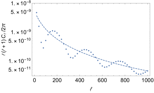
Figure 2: The behavior of the angular-power spectrum of CMB temperature fluctuations $C^{\text{BD}}_{\ell}$ (dotted line) and $C^{\text{cl}}_{\ell}$ (dashed line). $C_{\ell}^{\text{BD}}$ shows the oscillatory behavior and $C^{\text{cl}}_{\ell}$ does not have such a behavior.

Let us discuss how a model with free functions $m_{q}$ and $d_{q}$ defined in Eqs. (54) and (55) shows the oscillatory feature. The formula of the angular-power spectrum for $q\eta_{\text{m}}\gg 1$ is written by these functions as

$$C_{\ell}=\frac{8\pi}{2\ell+1}\int^{\infty}_{0}dq\,q^{2}\Bigl{[}(2m_{q}+1)|V_{\ell}(q)|^{2}-|d_{q}|\bigl{(}e^{i\theta_{q}}V^{2}_{\ell}(q)+e^{-i\theta_{q}}V^{*2}_{\ell}(q)\bigr{)}\Bigr{]},$$ (75)

where $d_{q}=|d_{q}|e^{i\theta_{q}}$ and $V_{\ell}(q)$ is given by (71). The second term of the integrand in (75) is crucial for the oscillatory feature. If the condition $m_{q}\gg|d_{q}|$ holds then the second term is negligible. Choosing $m_{q}$ as Eq. (62), we can get the almost same angular-power spectrum as that for the classical state. Also if the phase $\theta_{q}$ changes rapidly and takes various values in the $q$-integral, then the second term is neglected again by the Riemann-Lebesgue lemma. The PGWs superposed with many phases (the function $d_{q}$ controls the coherence of PGWs) contribute to the power spectrum, and the oscillation is reduced as a result. For the two situations $m_{q}\gg|d_{q}|$ or rapidly changing phase $\theta_{q}$, the oscillation degrades sufficiently even if the state has nonzero $d_{q}$, that is, nonzero discord. Therefore we can only conclude that the CMB power spectrum computed from the classical state has no oscillation. The converse statement that the absence of the oscillation means zero quantum discord does not necessarily hold.

The whole analysis is based on the free theory of the tensor perturbation, and the nonlinear interaction with other fields is not included. Since such nonlinear interactions can induce quantum decoherence generally, there is the possibility of loss of the quantum feature for PGWs. We discuss the decoherence effect for the tensor perturbation in the next section.

IV Decoherence for super-horizon modes and quantum correlations

Quantum decoherence is the loss of quantum superposition and induced by the interaction with an environment. In cosmological situations, quantum decoherence plays a crucial role to explain quantum-to-classical transition of primordial fluctuations. In Kiefer2007 , the authors discussed the decoherence for primordial fluctuations with the super-horizon modes and introduced the two conditions: the decoherence condition and the correlation condition. In this section, we clarify the meaning of these two conditions in terms of quantum correlations.

To get a clear intuition of the decoherence effect, we construct a decohered Gaussian state of PGWs. We consider the total system with the full Hamiltonian

$$\hat{H}(\eta)=\hat{H}^{y}_{0}(\eta)+\hat{H}^{\varphi}_{0}(\eta)+\hat{V}(\eta),$$ (76)

where $\hat{H}^{y}_{0}(\eta)$ and $\hat{H}^{\varphi}_{0}(\eta)$ are the free Hamiltonian of the tensor perturbation $\hat{y}_{ij}$ and the other fields $\hat{\varphi}$, respectively. The operator $\hat{V}(\eta)$ is the interaction between the tensor perturbation and the other fields. We assume that the initial state of the total system $\ket{\Psi}$ at $\eta\rightarrow-\infty$ is given by the product state

$$\ket{\Psi}=\ket{0^{\text{BD}}_{y}}\otimes\ket{\psi_{\varphi}},$$ (77)

where $\ket{0^{\text{BD}}_{y}}$ is the Bunch-Davies vacuum of the tensor field and $\ket{\psi_{\varphi}}$ is the initial state of the other fields. The wave functional of the total system is

$$\Psi_{\eta}[y,\varphi]=\bra{y,\varphi}\hat{U}(\eta,-\infty)\ket{\Psi},$$ (78)

where the time evolution operator $\hat{U}(\eta,-\infty)$ is expressed by using the time ordering as

$$\hat{U}(\eta,-\infty)=\text{T}\exp\left[-i\int^{\eta}_{-\infty}d\tau\hat{H}(\tau)\right].$$ (79)

We give the decohered state by assuming the following form of the reduced density matrix of $y_{\lambda}$ :

$$\rho_{\eta}[y,y^{\prime}]=\int_{\varphi}\Psi_{\eta}[y,\varphi]\Psi^{*}_{\eta}[y^{\prime},\varphi]=\Psi^{\text{BD}}_{\eta}[y](\Psi^{\text{BD}}_{\eta}[y^{\prime}])^{*}D_{\eta}[y,y^{\prime}],$$ (80)

with $\Psi^{\text{BD}}_{\eta}[y]$ and $D_{\eta}[y,y^{\prime}]$ are

$$\Psi^{\text{BD}}_{\eta}[y] =N(\eta)\exp\left[-\frac{1}{2}\sum_{\lambda=1,2}\int d^{3}q\,\Omega_{q}(\eta)|y_{\lambda}(\bm{q})|^{2}\right],$$ (81)

$$D_{\eta}[y,y^{\prime}] =\exp\left[-\frac{1}{2}\sum_{\lambda=1,2}\int d^{3}q\,\Gamma_{q}(\eta)|y_{\lambda}(\bm{q})-y^{\prime}_{\lambda}(\bm{q})|^{2}\right],$$ (82)

where $N(\eta)$ is the normalization and $\Omega_{q}(\eta)$ is given by (39). A phenomenological positive function $\Gamma_{q}(\eta)$ represents decoherence effect. The function $\Gamma_{q}$ depends on the structure of interaction with other fields $\varphi$. The decoherence factor $D_{\eta}[y,y^{\prime}]$ is invariant under spatial rotations and translations, which preserves the same symmetry imposed in the linear theory of PGWs. As $\Gamma_{q}$ becomes large, the off-diagonal components $\rho_{\eta}[y,y^{\prime}]$ decays exponentially. This behavior expresses quantum decoherence. The form of the decoherence factor $D_{\eta}[y,y^{\prime}]$ respects the facts that the field operator (growing mode) is the pointer observable Zurek1981 in cosmology. For super-horizon modes, in the Heisenberg picture, the field becomes constant in time and its conjugate momentum decays rapidly. Thus the field operator effectively commutes with the interaction Hamiltonian. Such an operator commuting with the interaction Hamiltonian is called a pointer observable. The density matrix of the system approaches diagonal form with respect to the basis of the pointer observable (pointer basis) by decoherence effect. In Kiefer2007 ; Burgess2008 ; Burgess2015 , for the super-horizon mode ($q\eta\ll 1$), the decoherence factor was derived using the quantum master equations with the Lindblad form Lindblad1976 ; Breuer2007 . Also the decoherence factor were computed from nonlinear interactions for primordial fluctuations in Nelson2016 ; Boyanovsky2016 ; Hollowood2017 .

In Kiefer2007 , the authors focused on the Wigner function of the density matrix of the decohered state and discussed its shape in the phase space. The density matrix $\rho(y,y^{\prime},\eta)$ for a fixed mode $\bm{q}$ and polarization $\lambda$ is

$$\rho(y,y^{\prime},\eta)=\psi^{\text{BD}}(y,\eta)[\psi^{\text{BD}}(y^{\prime},\eta)]^{*}\exp\left(-\Gamma_{q}|y-y^{\prime}|^{2}\right),$$ (83)

where $\psi^{\text{BD}}(y,\eta)$ is the wave function of the Bunch-Davies given in (39). The real part $\Omega^{\text{R}}_{q}$ characterizes the quantum superposition with respect to the field basis $y$. Such a superposition is suppressed by the decoherence factor if the parameter $\Gamma_{q}$ satisfies the inequality

$$\Gamma_{q}\gg\Omega_{q}^{\text{R}}.\qquad(\text{decoherence condition})$$ (84)

The decoherence degrades the superposition of the field amplitudes and makes the width of the Wigner function large in the direction of the conjugate momentum as follows. The Wigner function of the density matrix $\rho(y,y^{\prime},\eta)$ is

$$W(y,\pi_{y},\eta) =w(y^{\text{R}},\pi^{\text{R}}_{y},\eta)w(y^{\text{I}},\pi^{\text{I}}_{y},\eta),$$ (85)

$$w(x,p,\eta) =\sqrt{\frac{\Omega_{q}^{\text{R}}}{\pi^{2}(\Omega_{q}^{\text{R}}+2\Gamma_{q})}}\exp\left[-2\Omega_{q}^{\text{R}}\,x^{2}-2\frac{\left(p+\Omega_{q}^{\text{I}}\,x\right)^{2}}{\Omega_{q}^{\text{R}}+2\Gamma_{q}}\right].$$ (86)

For a large $\Gamma_{q}$, the Gaussian width for the conjugate momentum becomes large, and then Wigner ellipse approaches a circle. To observe the oscillation of the angular-power spectrum, the Wigner function should be squeezed even if decoherence occurs. In terms of the length of the major axis $a$ and the minor axis $b$ of the Wigner ellipse, the condition of squeezing Kiefer2007 is expressed as

$$a\gg b.\qquad(\text{correlation condition})$$ (87)

The word “correlation” does not mean quantum correlations but the correlation between the real (or imaginary) part of the field variable and its conjugate momentum.

In the following, we clarify the relation among the quantum correlations of PGWs at the matter era and the above conditions (84) and (87). For this purpose we consider the scenario that the decoherence due to the interaction halts just before the second horizon crossing of PGWs and the state of PGWs evolves unitarily after that. In this scenario, the decohered state of PGWs (83) is prepared at the conformal time $\eta_{\text{c}}$ which satisfies

$$\eta_{\text{r}}\leq\eta_{\text{c}},\quad q\,\eta_{\text{c}}=\epsilon,$$ (88)

where $\epsilon\sim 1$ is a model parameter. The whole evolution of PGWs in our setting is presented in Fig. 3.

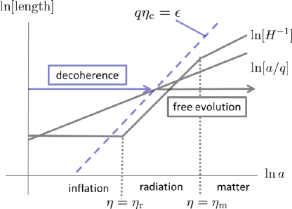
Figure 3: The assumption for the evolution of PGWs. Quantum decoherence continues until $\eta_{\text{c}}$ and then the PGW evolves unitarily.

We examine the decoherence condition (84) and the correlation condition (87) at $\eta=\eta_{\text{c}}$. To observe the decohered but squeezed state of PGWs, these conditions should be satisfied at the horizon crossing $\epsilon\sim 1$. For a super-horizon mode at $\eta_{r}$, $q\eta_{\text{r}}\ll 1$, the decoherence condition is estimated as

$$\frac{1}{|\beta_{q}|^{2}}\ll\frac{\Gamma_{q}(\eta_{\text{c}})}{q}$$ (89)

and the correlation condition is given as

$$\frac{\Gamma_{q}(\eta_{\text{c}})}{q}\ll|\beta_{q}|^{2},$$ (90)

where $\beta_{q}$ is the Bogolyubov coefficient given in (27).

Let us investigate the entanglement and quantum discord of PGWs in the matter era. For $\eta,\eta^{\prime}>\eta_{c}$, we have the two-point function $\langle yy\rangle$

$$\bra{\Psi}\hat{y}^{\text{H}}_{\lambda}(\bm{q},\eta)\hat{y}^{\text{H}}_{\lambda^{\prime}}(\bm{q}^{\prime},\eta^{\prime})\ket{\Psi}=\bra{\Psi}\hat{\Omega}^{\dagger}(\eta_{\text{c}},-\infty)\hat{y}^{\text{I}}_{\lambda}(\bm{q},\eta)\hat{y}^{\text{I}}_{\lambda^{\prime}}(\bm{q}^{\prime},\eta^{\prime})\hat{\Omega}(\eta_{\text{c}},-\infty)\ket{\Psi},$$ (91)

where $\hat{y}^{\text{H}}_{\lambda}$ and $\hat{y}^{\text{I}}_{\lambda}$ are the tensor field in the Heisenberg and interaction picture, respectively and $\hat{\Omega}(\eta,-\infty)$ is given by

$$\hat{\Omega}(\eta,-\infty)=\text{T}\exp\left[-i\int^{\eta}_{-\infty}d\tau\hat{V}^{\text{I}}(\tau)\right].$$ (92)

The concrete expression of the interaction Hamiltonian is not needed because the reduced density matrix of the tensor field (80) is given at $\eta_{\text{c}}$. In Eq. (91), we assumed that the interaction continues until $\eta_{\text{c}}$, that is, $\hat{\Omega}(\eta,-\infty)=\hat{\Omega}(\eta_{\text{c}},-\infty)$ for $\eta_{c}\leq\eta$. The field operator $\hat{y}^{\text{I}}_{\lambda}(\bm{q},\eta)$ can be written by the linear combination of $\hat{y}^{\text{I}}_{\lambda}(\bm{q},\eta_{\text{c}})$ and $\hat{\pi}^{\text{I}}_{\lambda}(\bm{q},\eta_{\text{c}})$ at $\eta_{\text{c}}$ as

$$\hat{y}^{\text{I}}_{\lambda}(\bm{q},\eta)=X_{q}(\eta,\eta_{\text{c}})\hat{y}^{\text{I}}_{\lambda}(\bm{q},\eta_{\text{c}})+Y_{q}(\eta,\eta_{\text{c}})\hat{\pi}^{\text{I}}_{\lambda}(\bm{q},\eta_{\text{c}}),$$ (93)

where $X_{q}$ and $Y_{q}$ are defined by

$$X_{q}(\eta,\eta^{\prime}) =f_{q}(\eta)g^{*}_{q}(\eta^{\prime})+f^{*}_{q}(\eta)g_{q}(\eta^{\prime}),$$ (94)

$$Y_{q}(\eta,\eta^{\prime}) =i[f_{q}(\eta)f^{*}_{q}(\eta^{\prime})-f^{*}_{q}(\eta)f_{q}(\eta^{\prime})].$$ (95)

From the form of the density matrix at $\eta_{\text{c}}$ (80), the correlation functions of the tensor field at the time $\eta_{\text{c}}$ in the interaction picture can be computed as follows:

$$\bra{\Psi}\hat{\Omega}^{\dagger}(\eta_{\text{c}},-\infty)\hat{y}^{\text{I}}_{\lambda}(\bm{q},\eta_{\text{c}})\hat{y}^{\text{I}}_{\lambda^{\prime}}(\bm{q}^{\prime},\eta_{\text{c}})\hat{\Omega}(\eta_{\text{c}},-\infty)\ket{\Psi} =\bra{0^{\text{BD}}_{y}}\hat{y}^{\text{I}}_{\lambda}(\bm{q},\eta_{\text{c}})\hat{y}^{\text{I}}_{\lambda^{\prime}}(\bm{q}^{\prime},\eta_{\text{c}})\ket{0^{\text{BD}}_{y}},$$ (96)

$$\bra{\Psi}\hat{\Omega}^{\dagger}(\eta_{\text{c}},-\infty)\hat{y}^{\text{I}}_{\lambda}(\bm{q},\eta_{\text{c}})\hat{\pi}^{\text{I}}_{\lambda^{\prime}}(\bm{q}^{\prime},\eta_{\text{c}})\hat{\Omega}(\eta_{\text{c}},-\infty)\ket{\Psi} =\bra{0^{\text{BD}}_{y}}\hat{y}^{\text{I}}_{\lambda}(\bm{q},\eta_{\text{c}})\hat{\pi}^{\text{I}}_{\lambda^{\prime}}(\bm{q}^{\prime},\eta_{\text{c}})\ket{0^{\text{BD}}_{y}},$$ (97)

$$\bra{\Psi}\hat{\Omega}^{\dagger}(\eta_{\text{c}},-\infty)\hat{\pi}^{\text{I}}_{\lambda}(\bm{q},\eta_{\text{c}})\hat{\pi}^{\text{I}}_{\lambda^{\prime}}(\bm{q}^{\prime},\eta_{\text{c}})\hat{\Omega}(\eta_{\text{c}},-\infty)\ket{\Psi} =\bra{0^{\text{BD}}_{y}}\hat{\pi}^{\text{I}}_{\lambda}(\bm{q},\eta_{\text{c}})\hat{\pi}^{\text{I}}_{\lambda^{\prime}}(\bm{q}^{\prime},\eta_{\text{c}})\ket{0^{\text{BD}}_{y}}$$

$$+\Gamma_{q}(\eta_{\text{c}})\delta_{\lambda\lambda^{\prime}}\delta^{3}(\bm{q}+\bm{q}^{\prime}).$$ (98)

The derivation of these equations is presented in the appendix C. Substituting Eq. (93) into the correlator (91) and using the formulas (96), (97) and (98), we obtain the correlator (91) for the different time $\eta$ and $\eta^{\prime}$ as

$$\bra{\Psi}\hat{y}^{\text{H}}_{\lambda}(\bm{q},\eta)\hat{y}^{\text{H}}_{\lambda^{\prime}}(\bm{q}^{\prime},\eta^{\prime})\ket{\Psi} =\bra{0^{\text{BD}}_{y}}\hat{y}^{\text{I}}_{\lambda}(\bm{q},\eta)\hat{y}^{\text{I}}_{\lambda^{\prime}}(\bm{q}^{\prime},\eta^{\prime})\ket{0^{\text{BD}}_{y}}$$

$$+Y_{q}(\eta,\eta_{\text{c}})Y_{q}(\eta^{\prime},\eta_{\text{c}})\Gamma_{q}(\eta_{\text{c}})\delta_{\lambda\lambda^{\prime}}\delta^{3}(\bm{q}+\bm{q}^{\prime}).$$ (99)

We can also calculate the other two-point functions $\langle y\pi\rangle$ and $\langle\pi\pi\rangle$. The conjugate momentum $\hat{\pi}^{\text{I}}_{\lambda}(\bm{q},\eta)$ is given by the following linear combination of $\hat{y}^{\text{I}}_{\lambda}(\bm{q},\eta_{\text{c}})$ and $\hat{\pi}^{\text{I}}_{\lambda}(\bm{q},\eta_{\text{c}})$:

$$\hat{\pi}^{\text{I}}_{\lambda}(\bm{q},\eta)=z_{q}(\eta,\eta_{\text{c}})\hat{y}^{\text{I}}_{\lambda}(\bm{q},\eta_{\text{c}})+w_{q}(\eta,\eta_{\text{c}})\hat{\pi}^{\text{I}}_{\lambda}(\bm{q},\eta_{\text{c}}),$$ (100)

where $z_{q}$ and $w_{q}$ are defined by

$$z_{q}(\eta,\eta^{\prime}) =(-i)\left[g_{q}(\eta)g^{*}_{q}(\eta^{\prime})-g^{*}_{q}(\eta)g_{q}(\eta^{\prime})\right],$$ (101)

$$w_{q}(\eta,\eta^{\prime}) =g_{q}(\eta)f^{*}_{q}(\eta^{\prime})+g^{*}_{q}(\eta)f_{q}(\eta^{\prime}).$$ (102)

Through the similar procedure, we can derive the other correlators as

$$\bra{\Psi}\hat{y}^{\text{H}}_{\lambda}(\bm{q},\eta)\hat{\pi}^{\text{H}}_{\lambda^{\prime}}(\bm{q}^{\prime},\eta^{\prime})\ket{\Psi} =\bra{0^{\text{BD}}_{y}}\hat{y}^{\text{I}}_{\lambda}(\bm{q},\eta)\hat{\pi}^{\text{I}}_{\lambda^{\prime}}(\bm{q}^{\prime},\eta^{\prime})\ket{0^{\text{BD}}_{y}}$$

$$+Y_{q}(\eta,\eta_{\text{c}})w_{q}(\eta^{\prime},\eta_{\text{c}})\Gamma_{q}(\eta_{\text{c}})\delta_{\lambda\lambda^{\prime}}\delta^{3}(\bm{q}+\bm{q}^{\prime}),$$ (103)

$$\bra{\Psi}\hat{\pi}^{\text{H}}_{\lambda}(\bm{q},\eta)\hat{\pi}^{\text{H}}_{\lambda^{\prime}}(\bm{q}^{\prime},\eta^{\prime})\ket{\Psi} =\bra{0^{\text{BD}}_{y}}\hat{\pi}^{\text{I}}_{\lambda}(\bm{q},\eta)\hat{\pi}^{\text{I}}_{\lambda^{\prime}}(\bm{q}^{\prime},\eta^{\prime})\ket{0^{\text{BD}}_{y}}$$

$$+w_{q}(\eta,\eta_{\text{c}})w_{q}(\eta^{\prime},\eta_{\text{c}})\Gamma_{q}(\eta_{\text{c}})\delta_{\lambda\lambda^{\prime}}\delta^{3}(\bm{q}+\bm{q}^{\prime}).$$ (104)

By Eqs. (99), (103) and (104), the correlators of $\hat{A}^{\text{H}}_{\lambda}$ and $\hat{A}^{\text{H}\dagger}_{\lambda}$ at $\eta$ are given by

$$\bra{\Psi}\hat{A}^{\text{H}\dagger}_{\lambda}(\bm{q},\eta)\hat{A}^{\text{H}}_{\lambda^{\prime}}(\bm{q}^{\prime},\eta)\ket{\Psi} =n^{\text{dec}}_{q}(\eta)\delta_{\lambda\lambda^{\prime}}\delta^{3}(\bm{q}-\bm{q}^{\prime}),$$ (105)

$$\bra{\Psi}\hat{A}^{\text{H}}_{\lambda}(\bm{q},\eta)\hat{A}^{\text{H}}_{\lambda^{\prime}}(\bm{q}^{\prime},\eta)\ket{\Psi} =c^{\text{dec}}_{q}(\eta)\delta_{\lambda\lambda^{\prime}}\delta^{3}(\bm{q}+\bm{q}^{\prime}),$$ (106)

where we introduced the following quantities

$$n^{\text{dec}}_{q}(\eta) :=n_{q}(\eta)+\left|\sqrt{\frac{q}{2}}\,Y_{q}(\eta,\eta_{\text{c}})+\frac{i}{\sqrt{2q}}w_{q}(\eta,\eta_{\text{c}})\right|^{2}\Gamma_{q}(\eta_{\text{c}}),$$ (107)

$$c^{\text{dec}}_{q}(\eta) :=c_{q}(\eta)+\left(\sqrt{\frac{q}{2}}\,Y_{q}(\eta,\eta_{\text{c}})+\frac{i}{\sqrt{2q}}w_{q}(\eta,\eta_{\text{c}})\right)^{2}\Gamma_{q}(\eta_{\text{c}}).$$ (108)

We focus on the target wave mode $1/\eta_{\text{m}}\ll q\ll 1/\eta_{\text{r}}$ (28) and examine the PPT criterion in the matter era $\eta>\eta_{\text{m}}$. The decohered state is the bipartite state with the mode $\bm{q}$ and $-\bm{q}$ defined by the annihilation operators $\hat{A}^{\text{H}}(\bm{q},\eta)$ and $\hat{A}^{\text{H}}(-\bm{q},\eta)$. For the sub-horizon mode, the operator $\hat{A}^{\text{H}}(\bm{q},\eta)$ is the counterpart of $\hat{b}_{\lambda}(\bm{q})$ due to the relation $\hat{A}^{\text{I}}\sim\hat{b}\exp(-iq\eta)$ (Eq. (30)). Using Eqs (107) and (108), we can rewrite the PPT criterion (59) $n^{\text{dec}}_{q}\geq|c^{\text{dec}}_{q}|$ as

$$\frac{\Gamma_{q}(\eta_{\text{c}})}{q}\geq\frac{n_{q}(\eta)}{|qY_{q}(\eta,\eta_{\text{c}})+iw_{q}(\eta,\eta_{\text{c}})|^{2}\,n_{q}(\eta_{\text{c}})-\text{Re}[c_{q}(\eta)(qY_{q}(\eta,\eta_{\text{c}})-iw_{q}(\eta,\eta_{\text{c}}))^{2}]}.$$ (109)

For $q\eta_{c}=\epsilon\sim 1$, this inequality is evaluated up to the numerical factor as

$$\frac{\Gamma_{q}(\eta_{\text{c}})}{q}\gtrsim 1,$$ (110)

where we used the approximated formulas (35), (36) and

$$qY_{q}(\eta,\eta_{\text{c}})+iw_{q}(\eta,\eta_{\text{c}})\sim ie^{-iq(\eta-\eta_{\text{c}})}$$ (111)

for a sub-horizon scale $q\eta\gg 1$.

For the target frequency $q\eta_{\text{r}}\ll 1$, the tensor fields have the large occupation number $|\beta_{q}|^{2}\gg 1$, and the PPT criterion (110) implies the decoherence condition (89)

$$\frac{\Gamma_{q}(\eta_{\text{c}})}{q}\gtrsim 1\quad\Longrightarrow\quad\frac{\Gamma_{q}(\eta_{\text{c}})}{q}\gg\frac{1}{|\beta_{q}|^{2}}$$ (112)

Hence the decoherence condition (89) is not sufficient to eliminate the entanglement of PGWs. Next we evaluate the degree of quantum coherence $c^{\text{dec}}_{q}(\eta)$ to examine the quantum discord of PGWs. For the target wave number $1/\eta_{\text{m}}\ll q\ll 1/\eta_{\text{r}}$, we can approximate the function $c^{\text{dec}}_{q}(\eta)$ as

$$c^{\text{dec}}_{q}(\eta)\sim-\left(|\beta_{q}|^{2}+\frac{\Gamma_{q}(\eta_{\text{c}})}{2q}e^{2i\epsilon}\right)e^{-2iq\eta},$$ (113)

where we applied the approximated formulas (35), (36) and (111) again. If the phenomenological parameter $\Gamma_{q}(\eta_{c})$ satisfies the correlation condition (90), then the decoherence effect is negligible in (113). In this case, the quantum coherence of the Bunch-Davies vacuum survives. Because the decohered state is a Gaussian state, the nonzero $c^{\text{dec}}_{q}$ implies quantum discord in the matter-dominated era. Hence the correlation condition given in Kiefer2007 means that the PGWs have a chance to keep the quantum discord in the matter-dominated era.

Let us demonstrate the behavior of the angular-power spectrum for the decohered state. By the formula (104), the angular-power spectrum $C^{\text{dec}}_{\ell}$ for the decohered state is given by

$$C^{\text{dec}}_{\ell}=C^{\text{BD}}_{\ell}+\Delta C_{\ell},$$ (114)

where the impact of the decoherence on the angular-power spectrum is represented as

$$\Delta C_{\ell}=\frac{8\pi}{2\ell+1}\int^{\infty}_{0}dqq^{2}\,\Gamma_{q}(\eta_{\text{c}})|W_{\ell}(q)|^{2},$$ (115)

with

$$W_{\ell}(q):=\frac{\sqrt{2}}{M_{\text{pl}}}\frac{1}{(2\pi)^{3/2}}\sqrt{\frac{\pi(2\ell+1)(\ell+2)!}{2(\ell-2)!}}\int^{\eta_{0}}_{\eta_{\text{L}}}\frac{d\eta}{a(\eta)}\frac{j_{\ell}(q(\eta_{0}-\eta))}{q^{2}(\eta_{0}-\eta)^{2}}w_{q}(\eta,\eta_{\text{c}}).$$ (116)

In principle, the function $\Gamma_{q}(\eta)$ can be determined by assuming nonlinear interactions with other fields. Since a macroscopic system easily decoheres, we can expect that the value of $\Gamma_{q}(\eta_{\text{c}})$ increases for the larger system. For simplicity we assume that $\Gamma_{q}(\eta_{\text{c}})$ per mode is proportional to the number density $|\beta_{q}|^{2}$, that is,

$$\frac{\Gamma_{q}(\eta_{\text{c}})}{q}=\gamma|\beta_{q}|^{2},$$ (117)

where $\gamma$ is a dimensionless positive constant. For $\gamma\sim 1$, the correlation condition (90) is violated. In Fig. 4, we present the behavior of $\ell(\ell+1)C^{\text{dec}}_{\ell}/2\pi$ for $\gamma=1.0$ and $\gamma=0.1$ with $\epsilon=0.5,1.0,1.5$. As have already mentioned, the decoherence changes the ellipse of the Wigner function to a circle and hence the observable oscillation is reduced. However, in the left panel of Fig. 4 for $\gamma=1.0$, we still observe the oscillation after the decoherence for the super-horizon mode $\epsilon=0.5$ even if the correlation condition (90) is violated. This is because the Wigner function of PGWs with the super-horizon mode is squeezed until the horizon crossing after the decoherence (see Fig. 5).

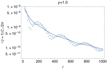
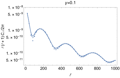
Figure 4: The anguler power spectrum of CMB fluctuations by PGWs with the decoherence effect (left panel: $\gamma=1.0$ and right panel: $\gamma=0.1$). The different curves correspond to $\epsilon=0.5$ (dotted line), $\epsilon=1.0$ (dashed line) and $\epsilon=1.5$ (solid line).

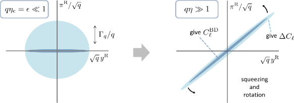
Figure 5: For the super-horizon mode, the Wigner function is squeezed until the mode re-enters the horizon after decoherence.

We observe that the oscillation vanishes for $\epsilon=1.5$. In this case, the Wigner ellipse becomes a circle and its shape does not change after the decoherence because of no squeezing effect for the sub-horizon modes. In the right panel of Fig. 4, we show the behavior of $\ell(\ell+1)C^{\text{dec}}_{\ell}/2\pi$ for $\gamma=0.1$. The oscillation does not vanish since the quantum discord of PGWs survives for $\gamma=0.1$ (in other words, the correlation condition is satisfied).

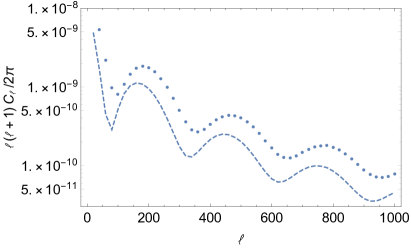
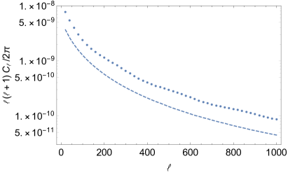
Figure 6: Left panel: $C^{\text{BD}}_{\ell}$ (dashed line) and $C^{\text{dec}}_{\ell}$ (dotted line) with $\epsilon=0.5$. Right panel: $C^{\text{cl}}_{\ell}$ (dashed line) and $C^{\text{dec}}_{\ell}$ (dotted line) with $\epsilon=1.5$.

In Fig. 6, we compare the angular-power spectrum for the Bunch-Davies vacuum and the classical state with the decoherence effect ($\gamma=1.0$). The left panel presents the behaviors of $C^{\text{BD}}_{\ell}$ and $C^{\text{dec}}_{\ell}$ with $\epsilon=0.5$ which show oscillation. The right panel shows the behaviors of $C^{\text{cl}}_{\ell}$ and $C^{\text{dec}}_{\ell}$ with $\epsilon=1.5$. The oscillations are reduced by the decoherence effect. In this case, $C^{\text{dec}}_{\ell}$ is almost $2C^{\text{cl}}_{\ell}$. For $\gamma=1.0$ and $\epsilon=1.5$, $\Delta C_{\ell}$ has the same amplitude and almost opposite phase as $C^{\text{BD}}_{\ell}$. That is $\Delta C_{\ell}$ can be evaluated by $C^{\text{BD}}_{\ell}$ using the mode function $e^{i\pi/2}v^{\text{rad}}_{q}$. Thus we find that

$$\Delta C_{\ell}\sim\frac{16\pi}{2\ell+1}\int^{\infty}_{0}dq\,q^{2}\,|\beta_{q}|^{2}\Bigl{[}|V_{\ell}(q)|^{2}-V^{2}_{\ell}(q)/2-V^{*2}_{\ell}(q)/2\Bigr{]},$$ (118)

and $C^{\text{dec}}_{\ell}=C^{\text{BD}}_{\ell}+\Delta C_{\ell}\sim 2C^{\text{cl}}_{\ell}$.

In Fig. 7, we summarize the relation among the entanglement, the quantum discord of PGWs, the decoherence condition and the correlation condition for super-horizon modes. As we have mentioned after Eq.  (59), the oscillation of the angular-power spectrum implies the quantum discord of PGWs but does not guarantees the existence of entanglement.

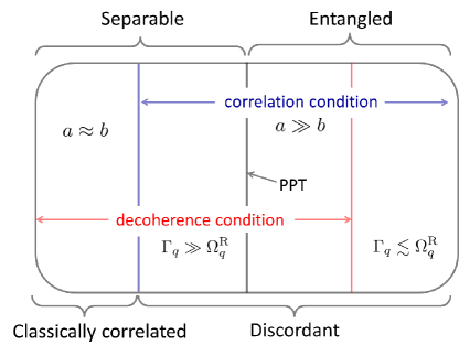
Figure 7: The relation among the quantum correlations of PGWs, the decoherence condition and the correlation condition. In the left side region of the red vertical line, the decoherence condition is satisfied. In the right side region of the blue vertical line, the correlation condition is satisfied.

For the decohered state, we can choose the parameter $\Gamma_{q}(\eta_{c})$ both satisfying the PPT criterion and the correlation condition. Thus it is also confirmed that the entanglement of PGWs is not required to obtain the oscillatory behavior of the angular-power spectrum of CMB fluctuations.

V Summary

Focusing on quantum correlations, we examined the oscillation of the angular-power spectrum of CMB fluctuations induced by PGWs. This oscillatory feature is different from the observed acoustic oscillation. The dominant contribution of the acoustic oscillation is due to primordial density perturbations not PGWs. However the oscillation caused by PGWs is related to the quantum discord of PGWs. We demonstrate that the constructed classical state of PGWs without quantum discord has no oscillatory feature for the angular-power spectrum of the CMB temperature fluctuations. For PGWs with quantum origin, the oscillation of the CMB power spectrum can be interpreted as the signature of the quantum discord of the PGWs.

We also investigated the decoherence effect for super-horizon modes on the squeezing property of PGWs. In particular, we discussed the decoherence condition and the correlation condition Kiefer2007 in terms of quantum correlations. Through the comparison of the PPT criterion and the decoherence condition, we found that the decoherece condition is not sufficient for the separability of the PGWs state in the matter-dominated era. Also we showed that the correlation condition implies the quantum discord of PGWs in the matter-dominated era. This argument is obvious because the correlation condition ensures the squeezed Wigner function if there is no decoherence after the horizon crossing. What we have done here is to furnish the meaning of the correlation condition in terms of quantum discord. We expect that the oscillatory feature of PGWs gives a hint for the question whether PGWs are quantum or not in our observable universe.

Appendix A Proof of the equation (56)

To show that the state satisfying the assumptions 2, 3, and 4 in the section III requires $d_{q}=0$, we consider a two-mode continuous variable state defined by two annihilation operators $\hat{a}_{\text{A}}$ and $\hat{a}_{\text{B}}$. Then we can prove the following lemma: a two-mode classically correlated Gaussian state $\rho_{\text{AB}}$ satisfies $\text{Tr}[\hat{a}_{\text{A}}\hat{a}_{\text{B}}\rho_{\text{AB}}]=\alpha_{\text{A}}\alpha_{\text{B}}$ where the parameters $\alpha_{\text{A,B}}$ are displacement of each system. By the assumption of classically correlated (Eq. (44)), the state $\rho_{\text{AB}}$ is represented as $\rho_{\text{AB}}=\sum_{i,j}p_{ij}\ket{\psi^{i}_{\text{A}}}\bra{\psi^{i}_{\text{A}}}\otimes\ket{\phi^{j}_{\text{B}}}\bra{\phi^{j}_{\text{B}}}$. Tracing out the system B, we have $\rho_{\text{A}}=\sum_{i}p_{i}\ket{\psi^{i}_{\text{A}}}\bra{\psi^{i}_{\text{A}}}$ where $p_{i}=\sum_{j}p_{ij}$. Since the state $\rho_{\text{AB}}$ is Gaussian, $\rho_{\text{A}}$ is a Gaussian state with the displacement $\alpha_{\text{A}}$. By the orthonormal property of $\ket{\psi^{i}_{\text{A}}}$, the vectors $\ket{\psi^{i}_{\text{A}}}$ are eigenvectors of the state $\rho_{\text{A}}$. From the Williamson theorem Williamson1936 , we can identify the state vector $\ket{\psi^{i}_{\text{A}}}$ with a state $\hat{D}_{\text{A}}(\alpha)\ket{N_{\text{A}}}$. Here $\hat{D}_{\text{A}}(\alpha)$ is the displacement operator of the system A. The parameter $\alpha_{\text{A}}$ does not depend on the label $i$, and $\ket{N_{\text{A}}}$ is an N-particle state defined by an annihilation operator $\hat{b}_{\text{A}}$, whose label $N$ corresponds to the label $i$ up to the ordering. Further, the Williamson theorem implies that there is the unitary operator generated by the symplectic transformation such that $\hat{a}_{\text{A}}=\xi_{\text{A}}\hat{b}_{\text{A}}+\eta_{\text{A}}\hat{b}^{\dagger}_{\text{A}}$ where $\xi_{\text{A}}$ and $\eta_{\text{A}}$ are the parameters of the symplectic transformation. The above statement holds for the system B. Hence we find the following equation

$$\text{Tr}[\hat{a}_{\text{A}}\hat{a}_{\text{B}}\rho_{\text{AB}}] =\sum_{i,j}p_{ij}\bra{\psi^{i}_{\text{A}}}\hat{a}_{\text{A}}\ket{\psi^{i}_{\text{A}}}\bra{\phi^{j}_{\text{B}}}\hat{a}_{\text{B}}\ket{\phi^{j}_{\text{B}}}$$

$$=\sum^{\infty}_{N,M=0}p_{NM}\bra{N_{\text{A}}}(\hat{a}_{\text{A}}+\alpha_{\text{A}})\ket{N_{\text{A}}}\bra{M_{\text{B}}}(\hat{a}_{\text{B}}+\alpha_{\text{B}})\ket{M_{\text{B}}}=\alpha_{\text{A}}\alpha_{\text{B}},$$ (119)

where we identified $\ket{\phi^{j}_{\text{B}}}$ with $\hat{D}_{\text{B}}(\alpha)\ket{M_{\text{B}}}$. $\hat{D}_{\text{B}}(\alpha)$ is the displacement operator for the system B and $\ket{M_{\text{B}}}$ is an M-particle state of the system B. The equation (119) implies that the Gaussian state is a product state.

Appendix B Derivation of the inequality (59)

We consider a two-mode Gaussian state $\rho_{\text{AB}}$, whose modes are defined by the annihilation operators $\hat{a}_{\text{A}}$ and $\hat{a}_{\text{B}}$. We introduce the vector $\hat{\alpha}=\left[\hat{a}_{\text{A}},\hat{a}^{\dagger}_{\text{A}},\hat{a}_{\text{B}},\hat{a}^{\dagger}_{\text{B}}\right]^{\text{T}}$. The covariance matrix of the state $\rho_{\text{AB}}$ is defined by the Hermitian matrix $C_{ij}=\frac{1}{2}\text{Tr}[\{\hat{\alpha}^{\dagger}_{i},\hat{\alpha}_{j}\}\,\rho_{\text{AB}}]$ where $\{\cdot,\cdot\}$ is the anti-commutator. The explicit form of the matrix $C$ is

$$C=\begin{bmatrix}\frac{1}{2}\langle\{\hat{a}^{\dagger}_{\text{A}},\hat{a}_{\text{A}}\}\rangle&\langle(\hat{a}^{\dagger}_{\text{A}})^{2}\rangle&\langle\hat{a}^{\dagger}_{\text{A}}\hat{a}_{\text{B}}\rangle&\langle\hat{a}^{\dagger}_{\text{A}}\hat{a}^{\dagger}_{\text{B}}\rangle\\ &\frac{1}{2}\langle\{\hat{a}_{\text{A}},\hat{a}^{\dagger}_{\text{A}}\}\rangle&\langle\hat{a}_{\text{A}}\hat{a}_{\text{B}}\rangle&\langle\hat{a}_{\text{A}}\hat{a}^{\dagger}_{\text{B}}\rangle\\ &&\frac{1}{2}\langle\{\hat{a}^{\dagger}_{\text{B}},\hat{a}_{\text{B}}\}\rangle&\langle(\hat{a}^{\dagger}_{\text{B}})^{2}\rangle\\ &&&\frac{1}{2}\langle\{\hat{a}_{\text{B}},\hat{a}^{\dagger}_{\text{B}}\}\rangle\end{bmatrix},$$ (120)

where $\langle\cdot\rangle=\text{Tr}[\cdot\,\rho_{\text{AB}}]$ and the omitted components are determined by the Hermiticity. The covariance matrix satisfies the following uncertainty relation: for any $z=[z_{1},z_{2},z_{3},z_{4}]^{\text{T}},z_{i}\in\mathbb{C}$,

$$z^{\dagger}Cz=\frac{1}{2}\text{Tr}[\{(z\cdot\hat{\alpha})^{\dagger},z\cdot\hat{\alpha}\}\,\rho_{\text{AB}}]=\text{Tr}[(z\cdot\hat{\alpha})^{\dagger}z\cdot\hat{\alpha}\rho_{\text{AB}}]+\frac{1}{2}z^{\dagger}\Omega z\geq\frac{1}{2}z^{\dagger}\Omega z,$$

that is $C\geq\frac{1}{2}\Omega$ where the matrix $\Omega$ is given by $[\hat{\alpha}_{j},\hat{\alpha}^{\dagger}_{k}]=\Omega_{jk}$. The partial transpose operation for the subsystem B is represented by $\hat{b}_{\text{A}}\rightarrow\hat{b}_{\text{A}}$ and $\hat{b}_{\text{B}}\rightarrow\hat{b}^{\dagger}_{\text{B}}$ Simon2000 . We denote the partial transposed matrix as $\widetilde{C}$. Then the inequality for the PPT criterion is $\widetilde{C}\geq\frac{1}{2}\Omega$. The state of interest has only the two expectation values

$$\langle\hat{a}^{\dagger}_{\text{A}}\hat{a}_{\text{A}}\rangle=\langle\hat{a}^{\dagger}_{\text{B}}\hat{a}_{\text{B}}\rangle=n,\quad\langle\hat{a}_{\text{A}}\hat{a}_{\text{B}}\rangle=c.$$ (121)

Then the covariance matrix $C$ and its partial transposed matrix $\widetilde{C}$ are computed as

$$C=\begin{bmatrix}n+\frac{1}{2}&0&0&c^{*}\\ 0&n+\frac{1}{2}&c&0\\ 0&c^{*}&n+\frac{1}{2}&0\\ c&0&0&n+\frac{1}{2}\end{bmatrix},\quad\widetilde{C}=\begin{bmatrix}n+\frac{1}{2}&0&c^{*}&0\\ 0&n+\frac{1}{2}&0&c^{*}\\ c&0&n+\frac{1}{2}&0\\ 0&c&0&n+\frac{1}{2}\end{bmatrix}.$$ (122)

From this formula of $\widetilde{C}$, we easily get the PPT criterion as $n\geq|c|$.

Appendix C Derivation of the equations (96), (97) and (98)

We compute the two-point functions of the decohered state (80). For convenience, we use the Schrödinger picture to calculate them:

$$\bra{\Psi}\hat{\Omega}^{\dagger}(\eta_{\text{c}},-\infty)\hat{y}^{\text{I}}_{\lambda}(\bm{q},\eta_{\text{c}})\hat{y}^{\text{I}}_{\lambda^{\prime}}(\bm{q}^{\prime},\eta_{\text{c}})\hat{\Omega}(\eta_{\text{c}},-\infty)\ket{\Psi} =\bra{\Psi}\hat{U}^{\dagger}(\eta_{\text{c}},-\infty)\hat{y}_{\lambda}(\bm{q})\hat{y}_{\lambda^{\prime}}(\bm{q}^{\prime})\hat{U}(\eta_{\text{c}},-\infty)\ket{\Psi},$$ (123)

$$\bra{\Psi}\hat{\Omega}^{\dagger}(\eta_{\text{c}},-\infty)\hat{y}^{\text{I}}_{\lambda}(\bm{q},\eta_{\text{c}})\hat{\pi}^{\text{I}}_{\lambda^{\prime}}(\bm{q}^{\prime},\eta_{\text{c}})\hat{\Omega}(\eta_{\text{c}},-\infty)\ket{\Psi} =\bra{\Psi}\hat{U}^{\dagger}(\eta_{\text{c}},-\infty)\hat{y}_{\lambda}(\bm{q})\hat{\pi}_{\lambda^{\prime}}(\bm{q}^{\prime})\hat{U}(\eta_{\text{c}},-\infty)\ket{\Psi},$$ (124)

$$\bra{\Psi}\hat{\Omega}^{\dagger}(\eta_{\text{c}},-\infty)\hat{\pi}^{\text{I}}(\bm{q},\eta_{\text{c}})\hat{\pi}^{\text{I}}(\bm{q}^{\prime},\eta_{\text{c}})\hat{\Omega}(\eta_{\text{c}},-\infty)\ket{\Psi} =\bra{\Psi}\hat{U}^{\dagger}(\eta_{\text{c}},-\infty)\hat{\pi}_{\lambda}(\bm{q})\hat{\pi}_{\lambda^{\prime}}(\bm{q}^{\prime})\hat{U}(\eta_{\text{c}},-\infty)\ket{\Psi},$$ (125)

where $\hat{y}_{\lambda}(\bm{q}):=\hat{y}^{\text{I}}_{\lambda}(\bm{q},-\infty)$ and $\hat{\pi}_{\lambda}(\bm{q}):=\hat{\pi}^{\text{I}}_{\lambda}(\bm{q},-\infty)$ are the field operators and its conjugate momentum in the Schrödinger picture and $\hat{U}$ is the evolution operator given by (79). The correlation function $\langle yy\rangle$ at the time $\eta_{\text{c}}$ is

$$\bra{\Psi}\hat{U}^{\dagger}(\eta_{\text{c}},-\infty)\hat{y}_{\lambda}(\bm{q})\hat{y}_{\lambda^{\prime}}(\bm{q}^{\prime})\hat{U}(\eta_{\text{c}},-\infty)\ket{\Psi}=\int_{y}\,y_{\lambda}(\bm{q})y_{\lambda^{\prime}}(\bm{q}^{\prime})\rho_{\eta_{\text{c}}}[y,y]$$

$$\qquad\qquad=\int_{y}\,y_{\lambda}(\bm{q})y_{\lambda^{\prime}}(\bm{q}^{\prime})|\Psi^{\text{BD}}_{\eta_{\text{c}}}[y]|^{2}=\bra{0^{\text{BD}}_{y}}\hat{y}^{\text{I}}_{\lambda}(\bm{q},\eta_{\text{c}})\hat{y}^{\text{I}}_{\lambda^{\prime}}(\bm{q}^{\prime},\eta_{\text{c}})\ket{0^{\text{BD}}_{y}}.$$ (126)

Similarly the other correlation functions $\langle y\pi\rangle$ and $\langle\pi\pi\rangle$ are computed as

$$\bra{\Psi}\hat{U}^{\dagger}(\eta_{\text{c}},-\infty)\hat{y}_{\lambda}(\bm{q})\hat{\pi}_{\lambda^{\prime}}(\bm{q}^{\prime})\hat{U}(\eta_{\text{c}},-\infty)\ket{\Psi}=\int_{y}\,y_{\lambda}(\bm{q})\Bigl{[}-i\frac{\delta}{\delta\tilde{y}_{\lambda^{\prime}}(-\bm{q}^{\prime})}\Bigr{]}\rho_{\eta_{\text{c}}}[\tilde{y},y]\Bigl{|}_{\tilde{y}=y}$$

$$\qquad\qquad=\int_{y}\,y(\bm{q})\Bigl{[}-i\frac{\delta\Psi^{\text{BD}}_{\eta_{\text{c}}}[y]}{\delta y_{\lambda^{\prime}}(-\bm{q}^{\prime})}\Bigr{]}\Psi^{\text{BD}*}_{\eta_{\text{c}}}[y]=\bra{0^{\text{BD}}_{y}}\hat{y}^{\text{I}}_{\lambda}(\bm{q},\eta_{\text{c}})\hat{\pi}^{\text{I}}(\bm{q}^{\prime},\eta_{\text{c}})\ket{0^{\text{BD}}_{y}},$$ (127)

and

$$\bra{\Psi}\hat{U}^{\dagger}(\eta_{\text{c}},-\infty)\hat{\pi}_{\lambda}(\bm{q})\hat{\pi}_{\lambda^{\prime}}(\bm{q}^{\prime})\hat{U}(\eta_{\text{c}},-\infty)\ket{\Psi}=\int_{y}\Bigl{[}i\frac{\delta}{\delta y_{\lambda}(-\bm{q})}\Bigr{]}\Bigl{[}-i\frac{\delta}{\delta\tilde{y}_{\lambda^{\prime}}(-\bm{q}^{\prime})}\Bigr{]}\rho_{\eta_{\text{c}}}[\tilde{y},y]\Bigl{|}_{\tilde{y}=y}$$

$$\qquad\qquad=\int_{y}\,\Bigl{[}-i\frac{\delta\Psi^{\text{BD}}_{\eta_{\text{c}}}[y]}{\delta y_{\lambda^{\prime}}(-\bm{q}^{\prime})}\Bigr{]}\Bigl{[}i\frac{\delta\Psi^{\text{BD}*}_{\eta_{\text{c}}}[y]}{\delta y_{\lambda}(-\bm{q})}\Bigr{]}+\Gamma_{q}(\eta_{\text{c}})\delta_{\lambda\lambda^{\prime}}\delta^{3}(\bm{q}+\bm{q}^{\prime})$$

$$\qquad\qquad=\bra{0^{\text{BD}}_{y}}\hat{\pi}^{\text{I}}_{\lambda}(\bm{q},\eta_{\text{c}})\hat{\pi}^{\text{I}}_{\lambda^{\prime}}(\bm{q}^{\prime},\eta_{\text{c}})\ket{0^{\text{BD}}_{y}}+\Gamma_{q}(\eta_{\text{c}})\delta_{\lambda\lambda^{\prime}}\delta^{3}(\bm{q}+\bm{q}^{\prime}),$$ (128)

where we used the functional representation of the conjugate momentum $\hat{\pi}_{\lambda}(\bm{q})=-i\delta/\delta y_{\lambda}(-\bm{q})$.

References

(1)
H. P. Breuer and F. Petruccione, “The Theory of Open Quantum Systems.”, (Oxford University Press, Oxford, 2007)
(2)
L. P. Grischuk and Yu. V. Sidorov, “On the quantum state of relic gravitons”, Class. Quantum. Grav. 6 L161(1989)
(3)
L. P. Grischuk and Yu. V. Sidorov, “Squeezed quantum stffates of relic gravitons and primordial density fluctuations”, Phys. Rev.D 42 3413 (1990)
(4)
B. Allen, E. E. Flanagan, and M. A. Papa, “Is the squeezing of relic gravitational waves produced by inflation detectable ?”, Phys. Rev.D 61, (2000) 024024.
(5)
S. Bose and L. P. Grishchuk, “Observational determination of squeezing in relic gravitational waves and primordial density perturbations”, Phys. Rev.D 66, (2002) 043529.
(6)
C. Kiefer, I. Lohmar, D. Polarski and A. A. Starobinsky, “Pointer states for primordial fluctuations in inflationary cosmology”, Class. Quantum Grav. 24 (2007) 1699
(7)
Y. Nambu, “Entanglement of quantum fluctuations in the inflationary
universe”, Phys. Rev. D78, (2008) 044023.
(8)
C. P. Burgess, R. Holman, and D. Hoover, “Decoherence of inflationary primordial fluctuations”, Phys. Rev. D77 (2008) 063534
(9)
Y. Nambu and Y. Ohsumi, “Classical and quantum correlations of scalar field in the inflationary universe”, Phys. Rev. D84, (2011) 044028
(10)
J. Maldacena, “Entanglement entropy in de Sitter space”,
J. High Energy Phys.02, (2012) 38.
(11)
S. Kanno, “Impact of quantum entanglement on spectrum of cosmological
fluctuations”, J. Cosmol. Astropart. Phys.2014, (2014)
029–029.
(12)
S. Kanno, J. P. Shock, and J. Soda, “Entanglement negativity in the
multiverse”, J. Cosmol. Astropart. Phys.2015, (2015)
015–015.
(13)
C. P. Burgess, R. Holman, G. Tasinato and M. Williams, “EFT beyond the horizon: stochastic inflation and how primordial quantum fluctuations go classical”,
J. High Energy Phys.03, (2015) 090.
(14)
E. A. Lim, “Quantum information of cosmological correlations”, Phys. Rev. D , 91, (2015) 083522
(15)
D. Boyanovsky, “Effective field theory during inflation. II. Stochastic dynamics and power spectrum suppression”, Phys. Rev. D , 93, (2016) 043501
(16)
J. Martin and V. Vennin, “Quantum discord of cosmic inflation: Can we show that CMB anisotropies are of quantum-mechanical origin?”, Phys. Rev. D 93, (2016) 023505
(17)
S. Kanno, J. P. Shock, and J. Soda, “Quantum discord in de Sitter space”, Phys. Rev. D 94, (2016) 125014
(18)
E. Nelson, “Quantum decoherence during inflation from
gravitational nonlinearities”. J. Cosmol. Astropart. Phys.03, (2016) 022
(19)
T. J. Hollowood and J. I. McDonald, “Decoherence, discord, and the quantum master equation for cosmological perturbations”, Phys. Rev. D 95, (2017) 103521
(20)
A. Matsumura and Y. Nambu, “Large scale quantum entanglement in de Sitter spacetime”, Phys. Rev. D 98, (2018) 025004
(21)
J. Williamson, “On the Algebraic Problem Concerning the Normal Forms of Linear Dynamical Systems”, Am. J. Math.58, (1936)
(22)
G. Lindblad, “On the generators of quantum dynamical semigroups”, Commun. Math. Phys.48 (1976) 119
(23)
W. H. Zurek, “Pointer basis of quantum apparatus: Into what mixture does the wave packet collapse?”, Phys. Rev. D24, (1981)
(24)
R. F. Werner, “Quantum states with Einstein-Podolsky-Rosen correlations admitting a hidden-variable model”,
Phys. Rev. A40, (1989) 4277.
(25)
A. Peres, “Separability Criterion for Density Matrices”,
Phys. Rev. Lett.77, (1996) 1413.
(26)
M. Horodecki, R. Horodecki, and P. Horodecki, “Separability
of mixed states: necessary and sufficient conditions”,
Phys. Lett. A223, (1996) 1-8.
(27)
R. Simon, “Peres-Horodecki Separability Criterion for Continuous Variable Systems”,
Phys. Rev. Lett.84, (2000) 2729.
(28)
G. Giedke, B. Kraus, M. Lewenstein, and J. I. Cirac, “Entanglement Criteria for All Bipartite Gaussian States”, Phys. Rev. Lett.87, (2001) 167904.
(29)
H. Ollivier and W. H. Zurek, “Quantum Discord: A Measure of the Quantumness of Correlations”, Phys. Rev. Lett.88, (2001) 017901
(30)
L. Henderson and V. Vedral, “Classical, quantum and total correlations”, J. Phys. A34, (2001) 6899.
(31)
J. Oppenheim, M. Horodecki, P. Horodecki, and R. Horodecki, “Thermodynamical Approach to Quantifying Quantum Correlations”, Phys. Rev. Lett.89, (2002) 180402
(32)
K. Fujikawa, “Separability criteria for continuous-variable systems”, Phys. Rev. A80, (2009) 012315.
(33)
P. Giorda and M. G. A. Paris, “Gaussian Quantum Discord”, Phys. Rev. Lett.105, (2010) 020503
(34)
G. Adesso and A. Datta, “Quantum versus Classical Correlations in Gaussian States”, Phys. Rev. Lett.105, (2010) 030501