Time-dependent optimized coupled-cluster method for multielectron dynamics II. A coupled electron-pair approximation

Abstract

We report the implementation of a cost-effective approximation method within the framework of time-dependent optimized coupled-cluster (TD-OCC) method [J. Chem. Phys. 148, 051101 (2018)] for real-time simulations of intense laser-driven multielectron dynamics. The method, designated as TD-OCEPA0, is a time-dependent extension of the simplest version of the coupled-electron pair approximation with optimized orbitals [J. Chem. Phys. 139, 054104 (2013)]. It is size extensive, gauge invariant, and computationally much more efficient than the TD-OCC with double excitations (TD-OCCD). We employed this method to simulate the electron dynamics in Ne and Ar atoms exposed to intense near infrared laser pulses with various intensities. The computed results, including high-harmonic generation spectra and ionization yields, are compared with those of various other methods ranging from uncorrelated time-dependent Hartree-Fock (TDHF) to fully-correlated (within the active orbital space) time-dependent complete-active-space self-consistent-field (TD-CASSCF). The TD-OCEPA0 results show a good agreement with TD-CASSCF ones for moderate laser intensities. For higher intensities, however, TD-OCEPA0 tends to overestimate the correlation effect, as occasionally observed for CEPA0 in the ground-state correlation energy calculations.

I introduction

In recent years there has been a significant breakthrough in the experimental techniques to measure and control the motions of electrons in atoms and molecules, for example, measurement of the delay in photoionization schultze2010 ; klunder2011probing , migration of charge in a chemical process belshaw2012observation ; calegari2014 and dynamical change of the orbital picture during the course of bond breaking or formation itatani2004 ; smirnova2009high ; haessler2010attosecond . Atoms and molecules interacting with laser pulses of intensity $10^{14}\,{\text{W}}/{\text{cm}}^{2}$ or higher in the visible to mid-infrared region, show highly nonlinear response to the fields such as above-threshold ionization (ATI), tunneling ionization, nonsequential double ionization (NSDI) and high-harmonic generation (HHG). All these phenomena are by nature nonperturbative protopapas1997atomic . The essence of the attosecond science lies in the HHG ivanovrev2009 ; agostini2004physics ; gallmann2012attosecond , one of the most successful means to generate ultrashort coherent light pulses in the wavelength ranging from extreme-ultraviolet (XUV) to the soft x-ray regions chang2016fundamentals ; zhao2012tailoring ; takahashi2013attosecond ; popmintchev2012bright , which can be used to unravel the electronic structure itatani2004 ; smirnova2009high or dynamics calegari2014 ; kraus2015measurement of many-body quantum systems. The HHG spectrum is characterized by a plateau where the intensity of the emitted light remains nearly constant up to many orders, followed by a sharp cutoff kli2010 .

A whole lot of numerical methods have been developed to understand atomic and molecular dynamics in the intense laser field (For a comprehensive review on various wavefunction-based methods for the study of laser-induced electron dynamics, see Ref. 18) to catch up with the progress in the experimental techniques. In principle, “the best” one could do is to solve the time-dependent Schrödinger equation (TDSE) to have an exact description. However, the exact solution of the TDSE is not feasible for systems containing more than two electrons parker1998intense ; parker2000time ; pindzola1998time ; laulan2003correlation ; ishikawa2005above ; feist2009probing ; ishikawa2012competition ; sukiasyan2012attosecond ; vanroose2006double ; horner2008classical . As a consequence, single-active electron (SAE) approximation has been widely used, in which the outermost electron is explicitly treated with the effect of the other electrons modeled by an effective potential. The SAE model has been successful in numerically exploring various high-field phenomena krause1992jl ; kulander1987time . However, the missing electron correlation in SAE makes this method at best qualitative. haessler2010attosecond

Among other established methods, the multiconfiguration time-dependent Hartree-Fock (MCTDHF) caillat2005correlated ; kato2004time ; nest2005multiconfiguration ; haxton2011multiconfiguration ; hochstuhl2011two and time-dependent complete-active-space self-consistent-field (TD-CASSCF) sato2013time ; sato2016time ; tikhomirov2017high are the most competent theoretical methods for the study of the laser-driven multielectron dynamics where both configuration interaction (CI) coefficients and the orbitals are propagated in time. The time-dependent (or optimized in the sense of time-dependent variational principle) orbital formulation widens the applicability of these methods by allowing to use a fewer number of orbitals than the case of fixed orbital treatments. Though powerful, the dilemma with these full CI-based methods is the applicability to large atomic or molecular systems due to the factorial escalation of the computational cost with respect to the number of electrons. To subjugate this difficulty, more approximate, thus computationally more efficient time-dependent multiconfiguration self-consistent-field (TD-MCSCF) methods have been developed, based on the truncated CI expansion within the chosen active orbital space miyagi2013time ; miyagi2014time ; haxton2015two ; sato2015time , compromising size extensivity.

To regain the size extensivity, the coupled-cluster expansion shavitt:2009 ; kummel:2003 ; crawford2007introduction of the time-dependent wavefunction emerges naturally as an alternative to the truncated CI expansion. The initial ideas of developing time-dependent coupled-cluster go back to as early as 1978 by Schönhammer and Gunnarsson schonhammer1978schonhammer , and Hoodbhoy and Negele hoodbhoy1978time ; hoodbhoy1979time . Here we take note of a few theoretical works on the time-dependent coupled-cluster method for time-independent Hamiltoniandalgaard1983some ; koch1990coupled ; takahashi1986time ; prasad1988time ; sebastian1985correlation and a few recent applications of the method with fixed orbitalspigg2012time ; nascimento2016linear . Huber and Klamroth huber2011explicitly were the first to apply the coupled-cluster method (with single and double excitations) to laser-driven dynamics of molecules, using time-independent orbitals and the CI wavefunction reconstructed from the propagated CC amplitudes to evaluate the expectation value of operators.

In 2012, Kvaal pioneered a time-dependent coupled-cluster method using time-dependent orbitals for electron dynamics, designated as orbital-adaptive time-dependent coupled-cluster (OATDCC) method kvaal2012ab . Based on Arponen’s bi-orthogonal formulation of the coupled-cluster theoryarponen1983variational , the OATDCC method is derived from the complex-analytic action functional using time-dependent biorthonormal orbitals. Recently, we have also developed time-dependent optimized coupled-cluster (TD-OCC) method sato2018communication based on the real action functional using time-dependent orthonormal orbitals. The TD-OCC method is a time-dependent extension of the orbital optimized coupled-cluster method popular in the stationary electronic structure theory scuseria1987optimization ; sherrill1998energies ; krylov1998size ; lindh2012optimized . It is not only size extensive, but also gauge invariant, and scales polynomially with respect to the number of active electrons $N$. Theoretical as well as numerical comparison of closely-related OATDCC and TD-OCC methods is yet to be done, and will be discussed elsewhere. (See Refs. 64 and 65 for recent theoretical accounts on orbital-optimized and time-dependent coupled-cluster methods, and Refs. 66 and 67 for the gauge-invariant coupled-cluster response theory with orthonormal and biorthonormal orbitals, respectively.)

We have implemented TD-OCC method with double excitations (TD-OCCD) and double and triple excitations (TD-OCCDT) within the chosen active spacesato2018communication , of which the computational cost scales as $N^{6}$ and $N^{8}$, respectively. Such scalings are milder than the factorial one in the MCTDHF and TD-CASSCF methods; nevertheless, a lower cost alternative within the TD-OCC framework is highly appreciated to further extend the applicability to heavier atoms and larger molecules interacting with intense laser fields.

One such low-cost model is a family of the methods called coupled-electron pair approximation (CEPA), originally introduced in 1970’s meyer1971ionization ; meyer1977methods ; werner1976pno ; ahlrichs1985coupled ; pulay1985variational ; ahlrichs1975pno ; koch1980comparison . In particular, the simplest version of the family, denoted as CEPA0 (See Sec. II for the definition.), is recently attracting a renewed attention wennmohs2008comparative ; neese2009efficient ; kollmar2010coupled ; malrieu2010ability due to its high cost-performance balance. The orbital-optimized version of this method (OCEPA0) has been also developed and applied to the calculation of, e.g, equilibrium geometries and harmonic vibrational frequencies of moleculesbozkaya2013orbital , which motivated us to extend it to the time-dependent problem.

In the present article, we report the implementation of the time-dependent, orbital-optimized version of the CEPA0 theory, hereafter referred to as TD-OCEPA0. Pilot applications to the simulation of induced dipole moment, high-harmonic spectra, and ionization probability in three different laser intensities for Ne and Ar are reported. We compare TD-OCEPA0 results with those of other methods ranging from uncorrelated TDHF, TD-MCSCF with a truncated CI expansion, TD-OCCD, and fully correlated TD-CASSCF, using the same number of active orbitals (except for TDHF) to quantitatively explore the performance of TD-OCEPA0. The computational cost of TD-OCEPA0 scales as $N^{6}$, which is formally the same as that of TD-OCCD; however as shown in Sec. II, one need not solve for the double deexcitation operator $\Lambda_{2}$, but it is sufficient to propagate the double excitation operator $T_{2}$ since $\Lambda_{2}$=$T_{2}^{\dagger}$. This leads to a great saving of the computational time as numerically demonstrated in Sec. III.

The manuscript is arranged as follows. A concise description of the TD-OCEPA0 method is presented in Sec. II. Section III discusses the computational results. Finally, we made our concluding remark in Sec. IV. We use Hartree atomic units unless stated otherwise, and Einstein convention is implied throughout for summation over orbital indices.

II Method

II.1 Background

We consider a system with $N$ electrons governed by the following Hamiltonian,

$$H = \sum_{i=1}^{N}h(\bm{r}_{i},\bm{p}_{i})+\sum_{i=1}^{N-1}\sum_{j=2}^{N}\frac{1}{|\bm{r}_{i}-\bm{r}_{j}|},$$ (1)

where $\bm{r}_{i}$ and $\bm{p}_{i}$ are the position and canonical momentum of an electron $i$. The corresponding second quantized Hamiltonian reads

$$\hat{H} = h^{\mu}_{\nu}\hat{E}^{\mu}_{\nu}+\frac{1}{2}u^{\mu\gamma}_{\nu\lambda}\hat{E}^{\mu\gamma}_{\nu\lambda},$$ (2)

where $\hat{E}^{\mu}_{\nu}=\hat{c}^{\dagger}_{\mu}\hat{c}_{\nu}$ and $\hat{E}^{\mu\gamma}_{\nu\lambda}=\hat{c}^{\dagger}_{\mu}\hat{c}^{\dagger}_{\gamma}\hat{c}_{\lambda}\hat{c}_{\nu}$, with $\hat{c}^{\dagger}_{\mu}$ ($\hat{c}_{\mu}$) being a creation (annihilation) operator in a complete, orthonormal set of $2n_{\rm bas}$ spin-orbitals $\{\psi_{\mu}\}$, where $n_{\rm bas}$ is the number of basis functions (or the number of grid points) to expand the spatial part of $\psi_{\mu}$, and

$$h^{\mu}_{\nu}=\int dx_{1}\psi^{*}_{\mu}(x_{1})h(\bm{r}_{1},\bm{p}_{1})\psi_{\nu}(x_{1}),$$ (3)

$$u^{\mu\gamma}_{\nu\lambda}=\int\int dx_{1}dx_{2}\frac{\psi^{*}_{\mu}(x_{1})\psi^{*}_{\gamma}(x_{2})\psi_{\nu}(x_{1})\psi_{\lambda}(x_{2})}{|\bm{r}_{1}-\bm{r}_{2}|},$$ (4)

where $x_{i}=(\bm{r}_{i},\sigma_{i})$ is a composite spatial-spin coordinate.

The complete set of $2n_{\rm bas}$ spin-orbitals (labeled with $\mu,\nu,\gamma,\lambda$) is divided into $n_{\rm occ}$ occupied ($o,p,q,r,s$) and $2n_{\rm bas}-n_{\rm occ}$ virtual spin-orbitals having nonzero and vanishing occupations, respectively, in the coupled-cluster (or MCSCF) expansion of the total wavefunction. The occupied spin-orbitals are classified into $n_{\rm core}$ core spin-orbitals which are occupied in the reference $\Phi$ and kept uncorrelated, and $n_{\rm act}=n_{\rm occ}-n_{\rm core}$ active spin-orbitals ($t,u,v,w$) among which the $N_{\rm act}=N-n_{\rm core}$ active electrons are correlated. The active spin-orbitals are further splitted into those in the hole space ($i,j,k,l$) and the particle space ($a,b,c,d$), which are occupied and unoccupied, respectively, in $\Phi$. The core spin-orbitals can also be splitted into those in the frozen-core space ($i^{\prime\prime},j^{\prime\prime}$) which are fixed in time, and the dynamical-core space ($i^{\prime},j^{\prime}$) which are propagated in timesato2013time .

Hereafter we refer to spin-orbitals simply as orbitals. [Note that Refs. 36; 42; 37 for TD-MCSCF methods deal with the equations of motion (EOMs) for spatial orbitals.] The system Hamiltonian (2) is equivalently written as

$$\hat{H} = E_{0}+f^{\mu}_{\nu}\{\hat{E}^{\mu}_{\nu}\}+\frac{1}{4}v^{\mu\gamma}_{\nu\lambda}\{\hat{E}^{\mu\gamma}_{\nu\lambda}\},$$ (5)

where $E_{0}=\langle\Phi|\hat{H}|\Phi\rangle$, $f^{\mu}_{\nu}=h^{\mu}_{\nu}+v^{\mu j}_{\nu j}$ ($j$ running over core and hole spaces), $v^{\mu\gamma}_{\nu\lambda}=u^{\mu\gamma}_{\nu\lambda}-u^{\mu\gamma}_{\lambda\nu}$, and the bracket $\{\cdots\}$ implies that the operator inside is normal ordered relative to the reference.

II.2 Review of TD-OCC method

Let us begin with a generic TD-OCC framework, which relies on the time-dependent variational principle with real action functionalsato2018communication ,

$$S = \operatorname{Re}\int_{t_{0}}^{t_{1}}Ldt=\frac{1}{2}\int_{t_{0}}^{t_{1}}\left(L+L^{*}\right)dt,$$ (6)

$$L = \langle\Phi|(1+\hat{\Lambda})e^{-\hat{T}}(\hat{H}-i\frac{\partial}{\partial t})e^{\hat{T}}|\Phi\rangle,$$ (7)

where

$$\hat{T} = \hat{T}_{2}+\hat{T}_{3}\cdots=\tau^{ab}_{ij}\hat{E}^{ab}_{ij}+\tau^{abc}_{ijk}\hat{E}^{abc}_{ijk}\cdots,$$ (8)

$$\hat{\Lambda} = \hat{\Lambda}_{2}+\hat{\Lambda}_{3}\cdots=\lambda_{ab}^{ij}\hat{E}_{ab}^{ij}+\lambda_{abc}^{ijk}\hat{E}_{abc}^{ijk}\cdots,$$ (9)

with $\tau^{ab\cdots}_{ij\cdots}$ and $\lambda_{ab\cdots}^{ij\cdots}$ being excitation and deexcitation amplitudes, respectively. We require that the action to be stationary, $\delta S=0$, with respect to the variation of amplitudes $\delta\tau^{ab\cdots}_{ij\cdots}$, $\delta\lambda_{ab\cdots}^{ij\cdots}$ and orthonormality-conserving orbital variations $\delta\psi_{\mu}=\psi_{\nu}\Delta^{\nu}_{\mu}$, with antiHermitian matrix elements $\Delta^{\nu}_{\mu}\equiv\langle\psi_{\nu}|\delta\psi_{\mu}\rangle$.

To facilitate formulation of TD-OCEPA0 below, we transform the Lagrangian into two equivalent expressions,

$$L = L_{0}+\langle\Phi|(1+\hat{\Lambda})[\{\hat{H}-i\hat{X}\}e^{\hat{T}}]_{c}|\Phi\rangle-i\lambda^{ij\cdots}_{ab\cdots}\dot{\tau}^{ab\cdots}_{ij\cdots},$$ (10b)

$$= (h^{p}_{q}-iX^{p}_{q})\rho^{q}_{p}+\frac{1}{2}u^{pr}_{qs}\rho_{pr}^{qs}-i\lambda^{ij\cdots}_{ab\cdots}\dot{\tau}^{ab\cdots}_{ij\cdots},$$

where $\hat{X}=X^{\mu}_{\nu}\hat{E}^{\mu}_{\nu}$ with $X^{\mu}_{\nu}=\langle\psi_{\mu}|\dot{\psi}_{\nu}\rangle$ being antiHermitian, $L_{0}=\langle\Phi|(\hat{H}-i\hat{X})|\Phi\rangle$, and the symbol $[\cdots]_{c}$ indicates the restriction to diagrammatically connected terms. The one-electron and two-electron reduced density matrices (RDMs) $\rho^{q}_{p}$ and $\rho^{qs}_{pr}$ are defined, respectively, by

$$\rho^{q}_{p} = \langle\Phi|(1+\hat{\Lambda})e^{-\hat{T}}\hat{E}^{p}_{q}e^{\hat{T}}|\Phi\rangle,$$ (11)

$$\rho^{qs}_{pr} = \langle\Phi|(1+\hat{\Lambda})e^{-\hat{T}}\hat{E}^{pr}_{qs}e^{\hat{T}}|\Phi\rangle.$$ (12)

To benefit later discussions, we separate the one-electron and two-electron RDMs (1RDM and 2RDM, respectively) into reference and correlation contributions,

$$\rho^{q}_{p} = (\rho_{0})^{q}_{p}+\gamma^{q}_{p},$$ (13)

$$\rho^{qs}_{pr} = (\rho_{0})^{qs}_{pr}+\gamma^{qs}_{pr},$$ (14)

where the reference contributions $(\rho_{0})^{q}_{p}=\delta^{q}_{j}\delta^{j}_{p}$ and $(\rho_{0})^{qs}_{pr}=\gamma^{q}_{p}\delta^{s}_{j}\delta^{j}_{r}+\gamma^{s}_{r}\delta^{q}_{j}\delta^{j}_{p}-\gamma^{q}_{r}\delta^{s}_{j}\delta^{j}_{p}-\gamma^{s}_{p}\delta^{q}_{j}\delta^{j}_{r}+\delta^{q}_{j}\delta^{j}_{p}\delta^{s}_{k}\delta^{k}_{r}-\delta^{s}_{j}\delta^{j}_{p}\delta^{q}_{k}\delta^{k}_{r}$ ($j,k$ running over core and hole spaces) are independent of the correlation treatment, and the correlation contributions are defined as

$$\gamma^{q}_{p} = \langle\Phi|(1+\hat{\Lambda})[\{\hat{E}^{p}_{q}\}e^{\hat{T}}]_{c}|\Phi\rangle,$$ (15a)

$$\gamma^{qs}_{pr} = \langle\Phi|(1+\hat{\Lambda})[\{\hat{E}^{pr}_{qs}\}e^{\hat{T}}]_{c}|\Phi\rangle.$$ (15b)

See Ref. 59 for the derivation of general TD-OCC EOMs based on the real-valued action principle outlined here.

II.3 TD-OCEPA0 method

Now we define the TD-OCEPA0 method by (i) including double (de)excitations only ($\hat{T}=\hat{T}_{2}$, $\hat{\Lambda}=\hat{\Lambda}_{2}$) and (ii) linearizing the exponential operator $e^{\hat{T}_{2}}$, in the normal-ordered, connected expression of the coupled-cluster Lagrangian [Eq. (LABEL:eq:Lag_amp)],

$$L = L_{0}+\langle\Phi|(1+\hat{\Lambda}_{2})[\{\hat{H}-i\hat{X}\}(1+\hat{T}_{2})]_{c}|\Phi\rangle-i\lambda^{ij}_{ab}\dot{\tau}^{ab}_{ij},$$

and, accordingly the correlation RDMs [Eqs. (15)],

$$\gamma^{q}_{p} = \langle\Phi|(1+\hat{\Lambda}_{2})[\{\hat{E}^{p}_{q}\}(1+\hat{T}_{2})]_{c}|\Phi\rangle,$$ (17a)

$$\gamma^{qs}_{pr} = \langle\Phi|(1+\hat{\Lambda}_{2})[\{\hat{E}^{pr}_{qs}\}(1+\hat{T}_{2})]_{c}|\Phi\rangle.$$ (17b)

Requiring $\delta S/\delta\lambda^{ij}_{ab}(t)=0$ and $\delta S/\delta\tau^{ab}_{ij}(t)=0$, respectively, using $L$ of Eq. (II.3) derives

$$i\dot{\tau}^{ab}_{ij} = \langle\Phi|\hat{E}^{ij}_{ab}[\{\hat{H}-i\hat{X}\}(1+\hat{T}_{2})]_{c}|\Phi\rangle$$ (18)

$$= v_{ij}^{ab}-p(ij)\bar{f}_{j}^{k}\tau_{ik}^{ab}+p(ab)\bar{f}_{c}^{a}\tau_{ij}^{cb}$$

$$+ \frac{1}{2}v_{cd}^{ab}\tau_{ij}^{cd}+\frac{1}{2}v_{ij}^{kl}\tau_{kl}^{ab}+p(ij)p(ab)v_{ic}^{ak}\tau_{kj}^{cb},$$

$$-i\dot{\lambda}^{ij}_{ab} = \langle\Phi|(1+\hat{\Lambda}_{2})[\{\hat{H}-i\hat{X}\}\hat{E}^{ab}_{ij}]_{c}|\Phi\rangle$$ (19)

$$= v_{ab}^{ij}-p(ij)\bar{f}_{k}^{i}\lambda_{ab}^{kj}+p(ab)\bar{f}_{a}^{c}\lambda_{cb}^{ij}$$

$$+ \frac{1}{2}v_{ab}^{cd}\lambda_{cd}^{ij}+\frac{1}{2}v_{kl}^{ij}\lambda_{ab}^{kl}+p(ij)p(ab)v_{kb}^{cj}\lambda_{ac}^{ik},$$

where $\bar{f}^{p}_{q}=f^{p}_{q}-iX^{p}_{q}$, and $p(\mu\nu)$ is the anti-symmetrizer; ${\color[rgb]{0,0,0}p(\mu\nu)}A_{\mu\nu}=A_{\mu\nu}-A_{\nu\mu}$. Comparing Eqs (18) and (19), and noting that the orbitals are orthonormal, one sees that the EOM for $\lambda_{ab}^{ij}$ is the complex conjugate of that for $\tau_{ij}^{ab}$, concluding that $\hat{\Lambda}_{2}=\hat{T}_{2}^{\dagger}$. As a result, the first and second terms of Eq. (II.3) are real, and

$$\operatorname{Im}\int_{t_{0}}^{t_{1}}Ldt = \frac{1}{2i}\int_{t_{0}}^{t_{1}}(L-L^{*})dt$$ (20)

$$= \frac{1}{2}\left\{\left|\tau^{ab}_{ij}(t_{1})\right|^{2}-\left|\tau^{ab}_{ij}(t_{0})\right|^{2}\right\}$$

is independent of the integration path and irrelevant in taking its variation. Therefore, given the orthonormal orbitals, $L$ is essentially real, and one could equally base oneself on

$$S = \int_{t_{0}}^{t_{1}}Ldt,$$ (21)

for TD-OCEPA0 ansatz. See Sec. II.4 below for more explicit account of this point.

Based on the natively real action functional $S$ of Eq. (21), the equation for $X^{\mu}_{\nu}=\langle\psi_{\mu}|\dot{\psi}_{\nu}\rangle$ is derived by requiring $\delta S/\delta\Delta^{\mu}_{\nu}=0$ using the Lagrangian expression of Eq. (10b) and RDMs of Eqs. (17) to obtain

$$i(X^{\nu}_{p}\rho^{p}_{\mu}-\rho^{\nu}_{p}X^{p}_{\mu}) = F^{\nu}_{p}\rho^{p}_{\mu}-\rho^{\nu}_{p}F_{p}^{\mu*},$$ (22)

where $F^{\mu}_{p}=\langle\psi_{\mu}|\hat{F}|\psi_{p}\rangle$,

$$\hat{F}|\psi_{p}\rangle = \hat{h}|\psi_{p}\rangle+\hat{W}^{r}_{s}|\psi_{q}\rangle\rho^{qs}_{or}(\rho^{-1})_{p}^{o},$$ (23)

$$W^{r}_{s}(x_{1}) = \int dx_{2}\frac{\psi^{*}_{r}(x_{2})\psi_{s}(x_{2})}{|\bm{r}_{1}-\bm{r}_{2}|}.$$ (24)

Subsequent analyses of Eq. (22) are parallel to those for TD-MCSCF methodsmiyagi2013time ; sato2015time , and one arrives at the orbital EOMs,

$$i|\dot{\psi_{p}}\rangle = (\hat{1}-\hat{P})\hat{F}|\psi_{p}\rangle+|\psi_{q}\rangle X^{q}_{p},$$ (25)

where $\hat{1}$ is the identity operator within the orbital space $\{\psi_{\mu}\}$, and $\hat{P}=\sum_{q}|\psi_{q}\rangle\langle\psi_{q}|$, with non-redundant orbital rotations determined by

$$i(\delta^{t}_{u}-\rho^{t}_{u})X^{u}_{i^{\prime}} = F^{t}_{i^{\prime}}-\rho^{t}_{u}F_{u}^{i^{\prime}\!*},$$ (26)

$$i(X^{a}_{j}\rho^{j}_{i}-\rho^{a}_{b}X^{b}_{i}) = F^{a}_{j}\rho^{j}_{i}-\rho^{a}_{b}F_{b}^{j*}.$$ (27)

A careful consideration of the frozen-core orbitals within the electric dipole approximation derives

$$iX_{\mu}^{i^{\prime\prime}} = \left\{\begin{array}[]{ll}0&\textrm{(length gauge)}\\ \boldsymbol{E}(t)\cdot\langle\psi_{i^{\prime\prime}}|\boldsymbol{r}|\psi_{\mu}\rangle&\textrm{(velocity gauge)}\\ \end{array}\right.,$$ (30)

where $\boldsymbol{E}$ is the external electric field, enabling gauge-invariant simulations with frozen-core orbitals.sato2016time

Redundant orbital rotations $\{X^{i^{\prime}}_{j^{\prime}}\}$, $\{X^{i}_{j}\}$, and, $\{X^{a}_{b}\}$ can be arbitrary antiHermitian matrix elements. In particular, if one chooses $X^{a}_{b}=X^{i}_{j}=0$, the term $-i\hat{X}$ is dropped in Eqs. (18) and (19). Again as a consequence of $\hat{\Lambda}_{2}=\hat{T}^{\dagger}_{2}$, both 1RDM and 2RDM are Hermitian, of which the algebraic expression of non-zero elements are given by

$$\gamma^{j}_{i} = -\frac{1}{2}\lambda^{kj}_{cd}\tau^{cd}_{ki},\gamma^{b}_{a}=\frac{1}{2}\lambda^{kl}_{ca}\tau^{cb}_{kl},$$ (31a)

$$\gamma^{cd}_{ab} = \frac{1}{2}\lambda^{kl}_{ab}\tau^{cd}_{kl},\gamma^{kl}_{ij}=\frac{1}{2}\lambda^{kl}_{cd}\tau^{cd}_{ij},$$ (31b)

$$\gamma^{ia}_{bj} = \lambda^{ki}_{cb}\tau^{ca}_{kj},\gamma^{ij}_{ab}=\lambda_{ab}^{ij},$$ (31c)

$$\gamma^{ab}_{ij} = \tau^{ab}_{ij}.$$ (31d)

In summary, the TD-OCEPA0 method is defined by the EOMs of $\hat{T}_{2}$ amplitudes [Eq. (18)] and orbitals [Eq. (25)], with the hole-particle mixing determined by solving Eq. (22) and RDMs given by Eqs. (31).

Table 1: The ground state total energies of Be and Ne atoms.

	Basis	Method	This work	PSI4psi4
Be	6-31G∗be_basis	HF	$-$14.5667  6405	$-$14.5667  6403
		CEPA0	$-$14.6192  0336	$-$14.6192  0335
		OCEPA0	$-$14.6196  5019	$-$14.6196  5018
		OCCD	$-$14.6138  6552
		OCCDT	$-$14.6139  4064
		FCI	$-$14.6139  4255	$-$14.6135  4253
Ne	cc-pVDZbe_basis	HF	$-$128.4887  7555	$-$128.4887  7555
		CEPA0	$-$128.6802  1409	$-$128.6802  1409
		OCEPA0	$-$128.6802  9009	$-$128.6802  9009
		OCCD	$-$128.6795  9316
		OCCDT	$-$128.6807  2135
		FCI	$-$128.6808  8113	$-$128.6808  8113

II.4 Relation to other ansatz

As the name suggests, the TD-OCEPA0 method is a time-dependent extension of the stationary OCEPA0 method. In the stationary case, it is known that CEPA0 ahlrichs1979many ; wennmohs2008comparative , D-MBPT($\infty$) bartlett1977comparison ; bartlett1979quartic , third-order expectation value coupled-cluster [XCC(3)] bartlett1988expectation , and the linearized CCD (LCCD) bartlett1981many energy functionals are all equivalent. The similar equivalence in the time-dependent case can be demonstrated by considering the Lagrangian of Eq. (7). In particular, the XCC Lagrangian can be written as

$$L = \frac{1}{\langle\Phi|e^{\hat{T}^{\dagger}}e^{\hat{T}}|\Phi\rangle}\langle\Phi|e^{\hat{T}^{\dagger}}(\hat{H}-i\frac{\partial}{\partial t})e^{\hat{T}}|\Phi\rangle$$

$$= \langle\Phi|\left[e^{\hat{T}^{\dagger}}(\hat{H}-i\frac{\partial}{\partial t})e^{\hat{T}}\right]_{sc}|\Phi\rangle$$

$$\sim \langle\Phi|[(1+\hat{T}^{\dagger})(\hat{H}-i\frac{\partial}{\partial t})(1+\hat{T})]_{sc}|\Phi\rangle,$$

$$= L_{0}+\langle\Phi|[(1+\hat{T}^{\dagger})\{\hat{H}-i\hat{X}\}(1+\hat{T})]_{sc}|\Phi\rangle-i\tau^{ab*}_{ij}\dot{\tau}^{ab}_{ij},$$

where $[\cdots]_{sc}$ restricts to strongly connected terms, and the third line introduces the XCC(3) approximation. This Lagrangian, which leads to the same working equations as derived in Sec. II.3 (with $\hat{\Lambda}_{2}={\color[rgb]{0,0,0}\hat{T_{2}}^{\dagger}}$), emphasizes the Hermitian nature of the TD-OCEPA0, of which a certain advantage over the standard non-Hermitian treatment is discussed in Ref. 88 in the stationary case.

The EOMs of the TD-OCEPA0 method is simpler than those of the closely-related TD-OCCD method (See Appendix A for algebraic details of the TD-OCCD method.) in that all terms quadratic to $\tau^{ab}_{ij}$ are absent in the $\hat{T}_{2}$ equation [comparing Eq. (18) and (36)] and in the 2RDM expression [comparing Eq. (31d) and (38d)]. It should also be noted that one need not solve for $\hat{\Lambda}_{2}$ for TD-OCEPA0 since $\hat{\Lambda}_{2}=\hat{T}^{\dagger}_{2}$, in contrast to the fact that Eq. (37) should be solved for TD-OCCD. These simplifications make TD-OCEPA0 computationally much more efficient than TD-OCCD, as numerically demonstrated in Sec. III.

III Numerical results and discussions

III.1 Ground-state energy

We have implemented the TD-OCEPA0 method for atom-centered Gaussian basis functions and spherical finite-element discrete variable representation (FEDVR) basis for atoms, both with spin-restricted and spin-unrestricted treatments, by modifying the TD-OCCD code described in Ref. 59. Exploiting the feasibility of the imaginary time relaxation to obtain the ground statesato2018communication , we first computed the ground-state energy of Be and Ne atoms with standard Gaussian basis sets, and compare the results with those obtained by PSI4 program package psi4 , in which the time-independent OCEPA0 method is implemented. To facilitate the comparison, the number of active spatial orbitals $n_{\rm act}/2$ are set to be the same as the number of basis functions $n_{\rm bas}$, since this is the only capability of the PSI4 program. In this case, there are no virtual orbitals (See Sec. II.2 for the definition.), and therefore, the first term of Eq. (25) vanishes. We also take an option of imaginary-propagating amplitudes only, with all orbitals frozen at the canonical HF solution, to obtain the fixed-orbital CEPA0 energy.

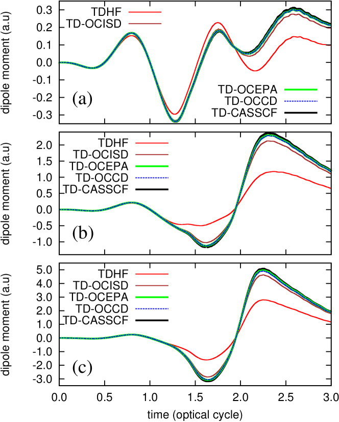
Figure 1: Time evolution of the dipole moment of Ne irradiated by a laser pulse of a wavelength of 800 nm and intensities of 5$\times$10¹⁴ W/cm² (a), 8$\times$10¹⁴ W/cm² (b), and 1$\times$10¹⁵ W/cm² (c), calculated with TDHF, TD-OCISD, TD-OCEPA, TD-OCCD, and TD-CASSCF methods.

Figure 2: Time evolution of the single ionization probability of Ne irradiated by a laser pulse of a wavelength of 800 nm and intensities of 5$\times$10¹⁴ W/cm² (a), 8$\times$10¹⁴ W/cm² (b), and 1$\times$10¹⁵ W/cm² (c), calculated with TDHF, TD-OCISD, TD-OCEPA, TD-OCCD, and TD-CASSCF methods.

The calculated total energies listed in Table 1 demonstrate a virtually perfect agreement of the results of this work and PSI4 program, both for CEPA0 and OCEPA0 methods and for Be and Ne atoms (with a small discrepancy due to a digit truncation of Gaussian one- and two-electron integrals), which confirms the correctness of our implementation.

It is also observed that, for both Be and Ne, the OCEPA0 energies are noticeably lower than the OCCD ones, and for the Be case, the OCEPA0 energy is slightly lower than the FCI energy. Such an overestimation of the correlation energy is usually considered not critical, and more than compensated by the size extensivity in the stationary case.

III.2 Application to electron dynamics in Ne and Ar

Next, we apply the TD-OCEPA0 method to the laser-driven electron dynamics in Ne and Ar atoms. Within the dipole approximation in the velocity gauge, the one-electron Hamiltonian is given by

$$h(\bm{r},\bm{p})=\frac{1}{2}|\bm{p}|^{2}-\frac{Z}{|\bm{r}|}+A(t)p_{z},$$ (33)

where $Z$ is the atomic number, $A(t)=-\int^{t}E(t^{\prime})dt^{\prime}$ is the vector potential, with $E(t)$ being the laser electric field linearly polarized along $z$ axis. It should be noted that TD-OCC method (including TD-OCEPA0) is gauge invariant; length-gauge and velocity-gauge simulations, upon numerical convergence, give the same result for observables. The velocity gauge employed here is advantageous in simulating high-field phenomenasato2016time ; orimo2018implementation .

The laser electric field is given by

$$E(t)=E_{0}\,{\text{sin}}(\omega_{0}t)\,{\text{sin}}^{2}\left(\pi\frac{t}{3T}\right),$$ (34)

for $0\leq t\leq 3T$, and $E(t)=0$ otherwise, with the central wavelength $\lambda=2\pi/\omega_{0}=800$ nm, the period $T=2\pi/\omega_{0}\sim 2.67$ fs, and the peak intensity $I_{0}=E_{0}^{2}$. We consider three different intensities 5$\times 10^{14}$ W/cm², 8$\times 10^{14}$ W/cm², and 1$\times 10^{15}$ W/cm² for Ne, and 2$\times 10^{14}$ W/cm², 4$\times 10^{14}$ W/cm², and 6$\times 10^{14}$ W/cm² for Ar.

The orbital functions are represented by the spherical FEDVR basissato2016time ; orimo2018implementation , with the maximum angular momentum $l_{\text{max}}=47$ for Ne and $l_{\text{max}}=63$ for Ar, and the FEDVR basis supporting the radial coordinate $0<r<240$ using 63 finite elements each containing 21 (for Ne) and 23 (for Ar) DVR functions. The absorbing boundary is implemented by a cos^1/4 mask function switched on at $r=180$ to avoid reflection from the box boundary. The ground state of each method is obtained by the imaginary time relaxation, and then the real-time dynamics are simulated starting from the ground state. The Fourth-order exponential Runge-Kutta method exponential_integrator is used to propagate the EOMs with 10000 time steps for each optical cycle.

We compare the performance of the following methods: (i) TDHF, (ii) TD-MCSCF with a TDHF determinant and singly and doubly excited configurations included (TD-OCISD), (iii) TD-OCCD, (iv) TD-OCCDT, and (iv) TD-CASSCF as the fully correlated reference for a given number of active orbitals. In all the methods, the 1$s$ orbital of Ne, and 1$s$2$s$2$p$ orbitals of Ar are kept frozen at the canonical Hartree-Fock orbitals, and for the correlated approaches (ii)-(iv) the eight valence electrons are correlated among 13 active orbitals. The method (ii) was first introduced in Ref. 40, and referred to as the time-dependent restricted-active-space self-consistent-field method. It can also be considered a specialization of more general time-dependent occupation-restricted multiple-active-space methodsato2016time . Here we denote the method as TD-OCISD (time-dependent optimized CI with singles and doubles) for simplicity.

The simulation results are given in Figs. 1-3 for Ne and Figs. 4-6 for Ar. For each atom, we report the time evolution of the dipole moment [Figs. 1 and 4], the ionization probability [Figs. 2 and 5], and the HHG spectra [Figs. 3 and 6]. The dipole moment is evaluated as a trace $\langle\psi_{p}|\hat{z}|\psi_{q}\rangle\rho^{q}_{p}$ using the 1RDM, and the ionization probability is defined as the probability of finding an electron outside a sphere of radius 20 a.u, computed by an expression using 1RDM and 2RDMLackner:2015 . The HHG spectrum is obtained as the modulus squared $I(\omega)=|a(\omega)|^{2}$ of the Fourier transform of the expectation value of the dipole acceleration, which, in turn, is obtained with a modified Ehrenfest expressionsato2016time . The TD-OCCDT results of the dipole moment and the ionization probability are not shown, since they meet a virtually perfect agreement with TD-CASSCF ones. The HHG spectrum is shown only for TDHF, TD-OCEPA0, TD-OCCD, and TD-CASSCF methods [Figs. 3(a)-(c) and 6(a)-(c)] to keep a visibility, and an absolute relative deviation

$$\delta(\omega)=\left|\frac{a(\omega)-a_{\textrm{TD-CASSCF}}(\omega)}{a_{\textrm{TD-CASSCF}}(\omega)}\right|$$ (35)

of the spectral amplitude $a(\omega)$ from the TD-CASSCF value is reported for each method [Figs. 3(d)-(f) and 6(d)-(f)]. Note that both $I(\omega)$ and $\delta(\omega)$ are plotted in the logarithmic scale, and $\delta(\omega)=1$ corresponds to a 100% deviation from the TD-CASSCF amplitude.

Figure 3: The HHG spectra from Ne irradiated by a laser pulse of a wavelength of 800 nm obtained with various methods (top), and the relative deviation of the spectral amplitude from the TD-CASSCF spectrum (bottom) defined as Eq. (35), for laser intensities of 5$\times$10¹⁴ W/cm² (a,d), 8$\times$10¹⁴ W/cm² (b,e), and 1$\times$10¹⁵ W/cm² (c,f).

Figure 4: Time evolution of the dipole moment of Ar irradiated by a laser pulse of a wavelength of 800 nm and intensities of 2$\times$10¹⁴ W/cm² (a), 4$\times$10¹⁴ W/cm² (b), and 6$\times$10¹⁴ W/cm² (c), calculated with TDHF, TD-OCISD, TD-OCEPA, TD-OCCD, and TD-CASSCF methods.

The dipole moment (Fig. 1) and the ionization probability (Fig. 2) of Ne atom show a general trend that the deviation of results for each method from TD-CASSCF ones decreases as TDHF $\gg$ TD-OCISD $>$ TD-OCEPA0 $\approx$ TD-OCCD $>$ TD-OCCDT. The HHG spectra [Fig. 3 (a)-(c)] are well reproduced by all the methods, except a systematic underestimation of the intensity by TDHF, with the magnitude of the error amounting to 100% of the TD-CASSCF spectral amplitude as shown in Fig. 3 (d)-(f). The magnitude of the error depends weakly on the harmonic order at the plateau region, which decreases again as TDHF $\gg$ TD-OCISD $>$ TD-OCEPA0 $\approx$ TD-OCCD $>$ TD-OCCDT. The Ne atom is characterized by its large ionization potential of 21.6 eV, resulting in relatively low ionization probabilities (Fig. 2) for the present laser pulses. In that case, TD-OCEPA0 and TD-OCCD give a notably similar, and accurate description of dynamics, implying that the truncation after the doubles amplitudes and the linearization of the Lagrangian [Eq. II.3] are both justified.

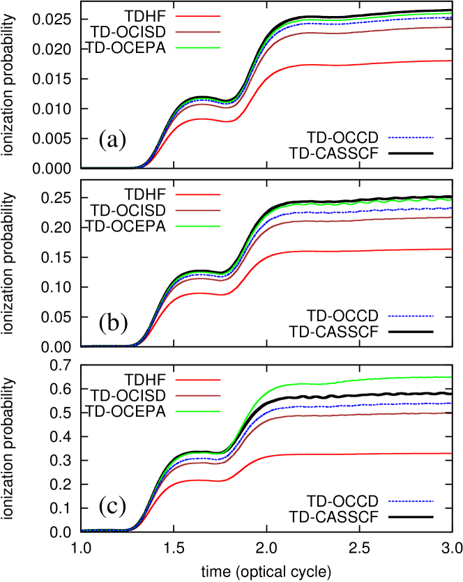
Figure 5: Time evolution of the single ionization probability of Ar irradiated by a laser pulse of a wavelength of 800 nm and intensities of 2$\times$10¹⁴ W/cm² (a), 4$\times$10¹⁴ W/cm² (b), and 6$\times$10¹⁴ W/cm² (c), calculated with TDHF, TD-OCISD, TD-OCEPA, TD-OCCD, and TD-CASSCF methods.

The Ar atom, having a lower ionization potential of 15.6 eV, exhibits a richer dynamics than Ne, e.g, a larger-amplitude oscillation of the dipole moment (Fig. 4), ionization probabilities as high as 70% (Fig. 5), and HHG spectra characterized by a dip around 34th harmonic related to the Cooper minimum of the photoionization spectrumWorner:2009 at the same energy (Fig. 6). The trend of the accuracy of each method is similar to the case for Ne, except that TD-OCEPA0 and TD-OCCD give noticeably different descriptions of dynamics. In general, TD-OCEPA0 tends to capture a larger part of the correlation effect (the difference between TDHF and TD-CASSCF) than TD-OCCD does. This results in, on one hand, a better agreement of the TD-OCEPA0 results (than TD-OCCD) with TD-CASSCF ones for lower intensity cases [Fig. 4 (a),(b), Fig. 5 (a),(b), and Fig. 6 (d),(e)], and, on the other, leads to an overestimation of the correlation effect for the highest intensity [Fig. 4 (c), Fig. 5 (c), Fig. 6 (f)], somewhat analogous to the overestimation of the ground-state correlation energy as discussed in Sec. III.1.

The nonlinear exponential parametrization in TD-OCCD seems to play a role in correcting the overestimation, and the inclusion of the triple excitations (TD-OCCDT) is essential to retain the decisive accuracy across the employed range of the laser intensity. Despite the aforementioned overestimation of the correlation effect for higher intensities, we judge that the present results of TD-OCEPA0 are quite encouraging; it clearly outperforms TD-OCISD for all properties of both atoms, and at least performs equally as TD-OCCD for a moderate laser intensity.

Figure 6: The HHG spectra from Ar irradiated by a laser pulse of a wavelength of 800 nm obtained with various methods (top), and the relative deviation of the spectral amplitude from the TD-CASSCF spectrum (bottom) defined as Eq. (35), for laser intensities of 2$\times$10¹⁴ W/cm² (a,d), 4$\times$10¹⁴ W/cm² (b,e), and 6$\times$10¹⁴ W/cm² (c,f)

Finally, we compare the computational cost of TD-OCEPA0 and TD-OCCD methods. Table 2 reports the central processor unit (CPU) time for the computational bottlenecks differing in these two methods, with varying numbers of active electrons and active orbitals. The largest active space with 18 electrons and 18 orbitals (18e-18o) is challenging for the fully correlated TD-CASSCF.

Table 2: Comparison of the CPU time (in second) spent for the evaluation of the $T_{2}$ equation, $\Lambda_{2}$ equation, and 2RDM for TD-OCCD and TD-OCEPA0 methods with various active spaces. See text for more details.

	TD-OCCD				TD-OCEPA0
active space	T2	$\Lambda_{2}$	2RDM		T2	$\Lambda_{2}$	2RDM
(8e-9o)	8.1	11.4	20.7		3.3	-	3.1
(8e-13o)	40.8	55.5	109.4		18.2	-	19.8
(8e-20o)	254.9	332.1	703.9		131.4	-	187.9
(14e-16o)	248.2	307.2	555.5		111.1	-	83.2
(16e-17o)	314.4	437.0	852.1		131.5	-	124.4
(18e-18o)	452.6	619.6	1024.8		187.9	-	143.3

First, depending on the active space configurations, the evaluation of the $\hat{T}_{2}$ equation of the TD-OCEPA0 [Eq. (18)] is 1.9$\sim$2.5 times faster than that of TD-OCCD [Eq. (36)]. A bigger computational gain comes from the fact that one need not solve for the $\Lambda_{2}$ equation, which, for TD-OCCD [Eq. (37)] takes longer than that for the $\hat{T}_{2}$ equation because of more mathematical operations involved. A further significant cost reduction is obtained by TD-OCEPA0 for the 2RDM evaluation [Eqs. (31d)], which is 5.5$\sim$7.2 times faster than the TD-OCCD case [Eqs. (38d)]. As a whole, the TD-OCEPA0 simulation with, e.g, the (18e-18o) active space achieves 6.3 times speed up relative to the TD-OCCD simulation with the same active orbital space.

IV Summary

We have presented the implementation of TD-OCEPA0 method as a cost-effective approximation within the TD-OCC framework, for the first principles study of intense laser-driven multielectron dynamics. The TD-OCEPA0 method retains the important size-extensivity and gauge-invariance of TD-OCC, and computationally much more efficient than the full TD-OCCD method. As a first numerical test, we applied the present implementation to Ne and Ar atoms irradiated by an intense near infrared laser pulses with three different intensities to compare the time-dependent dipole moment, the ionization probability, and HHG spectra with those obtained with other methods including the fully correlated TD-CASSCF methods with the same number of active orbitals. It is observed that, for the highest laser intensity, with sizable ionization, the TD-OCEPA0 tends to overestimate the correlation effect defined as the difference between TDHF and TD-CASSCF descriptions. For moderate intensities, however, the TD-OCEPA0 method performs at least equally well as TD-OCCD with a substantially lower computational cost. It is anticipated that the present TD-OCEPA0 method serves as an important theoretical tool to investigate ultrafast and/or high-field processes in chemically relevant large molecular systems.

Appendix A Algebraic details of TD-OCCD

The TD-OCCD method implemented in Ref. 59 employs the same truncation ($\hat{T}=\hat{T}_{2}$ and $\hat{\Lambda}=\hat{\Lambda}_{2}$) as for TD-OCEPA0, but retains the full exponential operator $e^{\hat{T}_{2}}$. As a result, the amplitude EOMs are given by

$$i\dot{\tau}^{ab}_{ij} = v_{ij}^{ab}-p(ij)\bar{f}_{j}^{k}\tau_{ik}^{ab}+p(ab)\bar{f}_{c}^{a}\tau_{ij}^{cb}$$ (36)

$$+ \frac{1}{2}v_{cd}^{ab}\tau_{ij}^{cd}+\frac{1}{2}v_{ij}^{kl}\tau_{kl}^{ab}+p(ij)p(ab)v_{ic}^{ak}\tau_{kj}^{cb}$$

$$- \frac{1}{2}p(ij)\tau_{ik}^{ab}\tau_{jl}^{cd}v_{cd}^{kl}+\frac{1}{2}p(ab)\tau_{ij}^{bc}\tau_{kl}^{ad}v_{cd}^{kl}$$

$$+ \frac{1}{4}\tau_{kl}^{ab}\tau_{ij}^{cd}v_{cd}^{kl}+\frac{1}{2}p(ij)p(ab)\tau_{il}^{bc}\tau_{jk}^{ad}v_{cd}^{kl},$$

$$-i\dot{\lambda}^{ij}_{ab} = v_{ab}^{ij}-p(ij)\bar{f}_{k}^{i}\lambda_{ab}^{kj}+p(ab)\bar{f}_{a}^{c}\lambda_{cb}^{ij}$$ (37)

$$+ \frac{1}{2}v_{ab}^{cd}\lambda_{cd}^{ij}+\frac{1}{2}v_{kl}^{ij}\lambda_{ab}^{kl}+p(ij)p(ab)v_{kb}^{cj}\lambda_{ac}^{ik}$$

$$- \frac{1}{2}p(ij)\lambda_{cd}^{ik}\tau^{cd}_{kl}v_{ab}^{jl}+\frac{1}{2}p(ab)\lambda_{bc}^{kl}\tau^{cd}_{kl}v_{ad}^{ij}$$

$$+ \frac{1}{4}\lambda_{ab}^{kl}\tau_{kl}^{cd}v_{cd}^{ij}+\frac{1}{2}p(ij)p(ab)\lambda_{ac}^{jk}\tau_{kl}^{cd}v_{bd}^{il}$$

$$- \frac{1}{2}p(ij)\lambda_{ab}^{ik}\tau_{kl}^{cd}v_{cd}^{jl}+\frac{1}{2}p(ab)\lambda_{bc}^{ij}\tau_{kl}^{cd}v_{ad}^{kl}$$

$$+ \frac{1}{4}\lambda_{cd}^{ij}\tau_{kl}^{cd}v_{ab}^{kl}.$$

The EOMs for orbitals are formally the same as that for TD-OCEPA0, Eqs. (25)-(27), but with RDMs $\rho$ replaced with Hermitialized ones, $D^{p}_{q}=(\rho^{p}_{q}+\rho^{q*}_{p})/2$ and $P^{pr}_{qs}=(\rho^{pr}_{qs}+\rho^{qs*}_{pr})/2$. Finally the algebraic expression for non-zero correlation RDM elements is

$$\gamma^{j}_{i} = -\frac{1}{2}\lambda^{kj}_{cd}\tau^{cd}_{ki},\gamma^{b}_{a}=\frac{1}{2}\lambda^{kl}_{ca}\tau^{cb}_{kl},$$ (38a)

$$\gamma^{cd}_{ab} = \frac{1}{2}\lambda^{kl}_{ab}\tau^{cd}_{kl},\gamma^{kl}_{ij}=\frac{1}{2}\lambda^{kl}_{cd}\tau^{cd}_{ij},$$ (38b)

$$\gamma^{ia}_{bj} = \lambda^{ki}_{cb}\tau^{ca}_{kj},\gamma^{ij}_{ab}=\lambda^{ij}_{ab},$$ (38c)

$$\gamma^{ab}_{ij} = \tau^{ab}_{ij}+\frac{1}{2}p(ij)p(ab)\lambda^{kl}_{cd}\tau^{ca}_{ki}\tau^{bd}_{jl}$$ (38d)

$$- \frac{1}{2}p(ij)\lambda^{kl}_{cd}\tau^{cd}_{ki}\tau^{ab}_{lj}-\frac{1}{2}p(ab)\lambda^{kl}_{cd}\tau^{ca}_{kl}\tau^{db}_{ij}$$

$$+ \frac{1}{4}\lambda^{kl}_{cd}\tau^{cd}_{ij}\tau^{ab}_{kl}.$$

References

- (1) M. Schultze et al., Science 328, 1658 (2010).
- (2) K. Klünder et al., Physical Review Letters 106, 143002 (2011).
- (3) L. Belshaw et al., The journal of physical chemistry letters 3, 3751 (2012).
- (4) F. Calegari et al., Science 346, 336 (2014).
- (5) J. Itatani et al., Nature 432, 867 (2004).
- (6) O. Smirnova et al., Nature 460, 972 (2009).
- (7) S. Haessler et al., Nature Physics 6, 200 (2010).
- (8) M. Protopapas, C. H. Keitel, and P. L. Knight, Reports on Progress in Physics 60, 389 (1997).
- (9) F. Krausz and M. Ivanov, Rev. Mod. Phys. 81, 163 (2009).
- (10) P. Agostini and L. F. DiMauro, Reports on progress in physics 67, 813 (2004).
- (11) L. Gallmann, C. Cirelli, and U. Keller, Annual review of physical chemistry 63, 447 (2012).
- (12) Z. Chang, Fundamentals of attosecond optics (CRC press, 2016).
- (13) K. Zhao et al., Optics letters 37, 3891 (2012).
- (14) E. J. Takahashi, P. Lan, O. D. Mücke, Y. Nabekawa, and K. Midorikawa, Nature communications 4, 2691 (2013).
- (15) T. Popmintchev et al., science 336, 1287 (2012).
- (16) P. M. Kraus et al., Science 350, 790 (2015).
- (17) K. L. Ishikawa, Advances in Solid State Lasers Development and Applications (InTech, 2010), chap. High-Harmonic Generation.
- (18) K. L. Ishikawa and T. Sato, IEEE Journal of Selected Topics in Quantum Electronics 21, 1 (2015).
- (19) J. S. Parker, E. S. Smyth, and K. T. Taylor, Journal of Physics B: Atomic, Molecular and Optical Physics 31, L571 (1998).
- (20) J. S. Parker et al., Journal of Physics B: Atomic, Molecular and Optical Physics 33, L239 (2000).
- (21) M. Pindzola and F. Robicheaux, Physical Review A 57, 318 (1998).
- (22) S. Laulan and H. Bachau, Physical Review A 68, 013409 (2003).
- (23) K. L. Ishikawa and K. Midorikawa, Physical Review A 72, 013407 (2005).
- (24) J. Feist et al., Physical review letters 103, 063002 (2009).
- (25) K. L. Ishikawa and K. Ueda, Physical review letters 108, 033003 (2012).
- (26) S. Sukiasyan, K. L. Ishikawa, and M. Ivanov, Physical Review A 86, 033423 (2012).
- (27) W. Vanroose, D. A. Horner, F. Martin, T. N. Rescigno, and C. W. McCurdy, Physical Review A 74, 052702 (2006).
- (28) D. A. Horner et al., Physical review letters 101, 183002 (2008).
- (29) J. Krause, Phys. Rev. Lett. 68, 3535 (1992).
- (30) K. C. Kulander, Physical Review A 36, 2726 (1987).
- (31) J. Caillat et al., Physical review A 71, 012712 (2005).
- (32) T. Kato and H. Kono, Chemical physics letters 392, 533 (2004).
- (33) M. Nest, T. Klamroth, and P. Saalfrank, The Journal of chemical physics 122, 124102 (2005).
- (34) D. J. Haxton, K. V. Lawler, and C. W. McCurdy, Physical Review A 83, 063416 (2011).
- (35) D. Hochstuhl and M. Bonitz, The Journal of chemical physics 134, 084106 (2011).
- (36) T. Sato and K. L. Ishikawa, Physical Review A 88, 023402 (2013).
- (37) T. Sato et al., Physical Review A 94, 023405 (2016).
- (38) I. Tikhomirov, T. Sato, and K. L. Ishikawa, Physical review letters 118, 203202 (2017).
- (39) H. Miyagi and L. B. Madsen, Physical Review A 87, 062511 (2013).
- (40) H. Miyagi and L. B. Madsen, Physical Review A 89, 063416 (2014).
- (41) D. J. Haxton and C. W. McCurdy, Physical Review A 91, 012509 (2015).
- (42) T. Sato and K. L. Ishikawa, Physical Review A 91, 023417 (2015).
- (43) I. Shavitt and R. J. Bartlett, Many-body methods in chemistry and physics: MBPT and coupled-cluster theory (Cambridge university press, 2009).
- (44) H. G. Kümmel, International Journal of Modern Physics B 17, 5311 (2003).
- (45) T. D. Crawford and H. F. Schaefer, Reviews in Computational Chemistry, Volume 14 , 33 (2007).
- (46) K. Schonhammer, Phys. Rev. B 18, 6606 (1978).
- (47) P. Hoodbhoy and J. W. Negele, Physical Review C 18, 2380 (1978).
- (48) P. Hoodbhoy and J. W. Negele, Physical Review C 19, 1971 (1979).
- (49) E. Dalgaard and H. J. Monkhorst, Physical Review A 28, 1217 (1983).
- (50) H. Koch and P. Jo/rgensen, The Journal of Chemical Physics 93, 3333 (1990).
- (51) M. Takahashi and J. Paldus, The Journal of chemical physics 85, 1486 (1986).
- (52) M. D. Prasad, The Journal of chemical physics 88, 7005 (1988).
- (53) K. Sebastian, Physical Review B 31, 6976 (1985).
- (54) D. A. Pigg, G. Hagen, H. Nam, and T. Papenbrock, Physical Review C 86, 014308 (2012).
- (55) D. R. Nascimento and A. E. DePrince III, Journal of chemical theory and computation 12, 5834 (2016).
- (56) C. Huber and T. Klamroth, The Journal of chemical physics 134, 054113 (2011).
- (57) S. Kvaal, The Journal of chemical physics 136, 194109 (2012).
- (58) J. Arponen, Annals of Physics 151, 311 (1983).
- (59) T. Sato, H. Pathak, Y. Orimo, and K. L. Ishikawa, The Journal of chemical physics 148, 051101 (2018).
- (60) G. E. Scuseria and H. F. Schaefer III, Chemical physics letters 142, 354 (1987).
- (61) C. D. Sherrill, A. I. Krylov, E. F. Byrd, and M. Head-Gordon, The Journal of chemical physics 109, 4171 (1998).
- (62) A. I. Krylov, C. D. Sherrill, E. F. Byrd, and M. Head-Gordon, The Journal of chemical physics 109, 10669 (1998).
- (63) G. D. Lindh, T. J. Mach, and T. D. Crawford, Chemical Physics 401, 125 (2012).
- (64) R. H. Myhre, The Journal of chemical physics 148, 094110 (2018).
- (65) T. B. Pedersen and S. Kvaal, The Journal of chemical physics 150, 144106 (2019).
- (66) T. B. Pedersen, H. Koch, and C. Hättig, The Journal of chemical physics 110, 8318 (1999).
- (67) T. B. Pedersen, B. Fernandez, and H. Koch, The Journal of chemical physics 114, 6983 (2001).
- (68) W. Meyer, International Journal of Quantum Chemistry 5, 341 (1971).
- (69) W. Meyer, Methods of electronic structure theory, 1977.
- (70) H.-J. Werner and W. Meyer, Molecular Physics 31, 855 (1976).
- (71) R. Ahlrichs, P. Scharf, and C. Ehrhardt, The Journal of Chemical Physics 82, 890 (1985).
- (72) P. Pulay and S. Sæbø, Chemical physics letters 117, 37 (1985).
- (73) R. Ahlrichs, F. Driessler, H. Lischka, V. Staemmler, and W. Kutzelnigg, The Journal of Chemical Physics 62, 1235 (1975).
- (74) S. Koch and W. Kutzelnigg, Theoretica chimica acta 59, 387 (1980).
- (75) F. Wennmohs and F. Neese, Chemical Physics 343, 217 (2008).
- (76) F. Neese, F. Wennmohs, and A. Hansen, The Journal of chemical physics 130, 114108 (2009).
- (77) C. Kollmar and F. Neese, Molecular Physics 108, 2449 (2010).
- (78) J.-P. Malrieu, H. Zhang, and J. Ma, Chemical Physics Letters 493, 179 (2010).
- (79) U. Bozkaya and C. D. Sherrill, The Journal of chemical physics 139, 054104 (2013).
- (80) J. M. Turney et al., Wiley Interdisciplinary Reviews: Computational Molecular Science 2, 556 (2012).
- (81) J. D. Dill and J. A. Pople, The Journal of Chemical Physics 62, 2921 (1975).
- (82) M. Frisch et al., Gaussian 09, revision d. 01, 2009.
- (83) R. Ahlrichs, Computer Physics Communications 17, 31 (1979).
- (84) R. J. Bartlett and I. Shavitt, Chemical Physics Letters 50, 190 (1977).
- (85) R. J. Bartlett, I. Shavitt, and G. D. Purvis III, The Journal of Chemical Physics 71, 281 (1979).
- (86) R. J. Bartlett and J. Noga, Chemical physics letters 150, 29 (1988).
- (87) R. J. Bartlett, Annual Review of Physical Chemistry 32, 359 (1981).
- (88) A. G. Taube and R. J. Bartlett, The Journal of chemical physics 130, 144112 (2009).
- (89) Y. Orimo, T. Sato, A. Scrinzi, and K. L. Ishikawa, Physical Review A 97, 023423 (2018).
- (90) M. Hochbruck and A. Ostermann, Acta Numerica 19, 209 (2010).
- (91) F. Lackner, I. Březinová, T. Sato, K. L. Ishikawa, and J. Burgdörfer, Physical Review A 91, 023412 (2015).
- (92) J. Wörner, Hans, H. Niikura, J. B. Bertrand, P. Corkum, and D. Villeneuve, Phys. Rev. Lett. 102, 103901 (2009).