Minimal entropy production due to constraints on rate matrix dependencies in multipartite processes

Abstract

I consider multipartite processes in which there are constraints on each subsystem’s rate matrix, restricting which other subsystems can directly affect its dynamics. I derive a strictly nonzero lower bound on the minimal achievable entropy production rate of the process in terms of these constraints on the rate matrices of its subsystems. The bound is based on constructing counterfactual rate matrices, in which some subsystems are held fixed while the others are allowed to evolve. This bound is related to the “learning rate” of stationary bipartite systems, and more generally to the “information flow” in bipartite systems.

Introduction.— Many systems are naturally modeled as having two or more interacting subsystems. Recent research in stochastic thermodynamics seifert2012stochastic ; van2015ensemble ; esposito2010three ; wolpert_thermo_comp_review_2019 has started to investigate such composite systems sagawa2008second ; sagawa2009minimal ; parrondo2015thermodynamics ; horowitz2014thermodynamics ; barato_efficiency_2014 ; ito2013information ; hartich_sensory_2016 . So far, most of the research has been on the special case of bipartite processes, i.e., systems composed of two co-evolving subsystems, which have zero probability of making a state transition simultaneously sagawa2008second ; sagawa2009minimal ; parrondo2015thermodynamics ; horowitz2014thermodynamics ; hartich_sensory_2016 ; barato_efficiency_2014 ; ito2013information ; fluct.theorems.partially.masked.shiraishi.sagawa.2015 ; Bisker_2017 ; shiraishi_ito_sagawa_thermo_of_time_separation.2015 . However, given that many systems have more than just two interacting subsystems, research is starting to extend to fully multipartite processes horowitz_multipartite_2015 ; ito2013information ; wolpert_book_2018 .

The definition of any composite system specifies which subsystems directly affect the dynamics of which other subsystems. It is now known that just by itself, such a specification of which subsystem affects which other one can cause a strictly positive lower bound on the entropy production rate (EP) of the overall composite system wolpert_thermo_comp_review_2019 ; wolpert2020thermodynamics ; Boyd:2018aa . This minimal EP has sometimes been called “Landauer loss”, because it is the extra EP beyond the minimal amount (namely, zero) implicit in the Landauer bound wolpert_thermo_comp_review_2019 ; wolpert2020thermodynamics ; wolpert_book_review_chap_2019

Previous analyses of Landauer loss focused on scenarios where every subsystem evolves in isolation, without any direct coupling to the other subsystems. This is a severe limitation of those analyses. As an illustration, consider a composite system with three subsystems $A,B$ and $C$. $B$ evolves independently of $A$ and $C$. However, $B$ is continually observed by $C$ as well as $A$. Moreover, suppose that $A$ is really two subsystems, $1$ and $2$. Only subsystem $2$ directly observes $B$, whereas subsystem $1$ observes subsystem $2$, e.g., to record a running average of the values of subsystem $2$ (see Fig. 1).

There has been some work on a simplified version of this scenario, in which subsystem $4$ is absent and subsystem $3$ is required to be at equilibrium hartich_sensory_2016 ; bo2015thermodynamic . But this work has focused on issues other than the minimal EP.

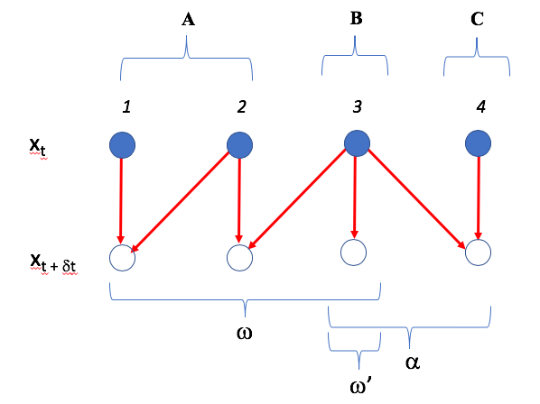
Figure 1: Four subsystems, $\{1,2,3,4\}$ interacting in a multipartite process. The red arrows indicate dependencies in the associated four rate matrices. $B$ evolves autonomously, but is continually observed by $A$ and $C$. So the statistical coupling between $A$ and $C$ could grow with time, even though their rate matrices do not involve one another. The three overlapping sets indicated at the bottom of the figure specify the three communities of a community structure for this process.

To investigate Landauer loss in these kinds of composite systems, here I model them as multipartite processes, in which each subsystem evolves according to its own rate matrix horowitz_multipartite_2015 . So restrictions on the direct coupling of any subsystem $i$ to the other subsystems are modeled as restrictions on the rate matrix of subsystem $i$, to only involve a limited set of other subsystems, called the “community” of $i$. (These are instead called “neighborhoods” in horowitz_multipartite_2015 , but that expression already means something in topology, and so I don’t use it here.)

In this paper I derive a lower bound on the Landauer loss rate of composite systems, by deriving an exact equation for that minimal EP rate as a sum of non-negative expressions. One of those expressions is related to quantities that were earlier considered in the literature. It reduces to what has been called the “learning rate” in the special case of stationary bipartite systems barato_efficiency_2014 ; Brittain_2017 ; hartich_sensory_2016 . That expression is also related to what (in a different context) has been called the “information flow” between a pair of subsystems horowitz2014thermodynamics ; horowitz_multipartite_2015 .

Rate matrix communities.— I write $\mathcal{N}$ for a particular set of $N$ subsystems, with finite state spaces $\{X_{i}:i=1,\ldots N\}$. $x$ indicates a vector in $X$, the joint space of $\mathcal{N}$. For any $A\subset\mathcal{N}$, I write $-A:=\mathcal{N}\setminus A$. So for example $x_{-A}$ is the vector of all components of $x$ other than those in $A$. A distribution over a set of values $x$ at time $t$ is written as $p^X(t)$, with its value for $x\in X$ written as $p^X_{x}(t)$, or just $p_{x}(t)$ for short. Similarly, $p^{X|Y}_{x,y}(t)$ is the conditional distribution of $X$ given $Y$ at time $t$, evaluated for the event $X=x,Y=y$ (which I sometimes shorten to $p_{x|y}(t)$). I write Shannon entropy as $S(p_{X}(t))$, $S_{t}(X)$, or $S^{X}(t)$, as convenient. I also write the conditional entropy of $X$ given $Y$ at $t$ as $S^{X|Y}(t)$. I write the Kronecker delta as both $\delta(a,b)$ or $\delta^a_{b}$.

The joint system evolves as a multi-partite process, there is a set of time-varying stochastic rate matrices, $\{K^{x^{\prime}}_{x}(i;t):i=1,\ldots,N\}$, where for all $i$, $K^{x^{\prime}}_{x}(i;t)=0$ if $x^{\prime}_{-i}\neq x_{-i}$, and where the joint dynamics over $X$ is governed by the master equation

$$\frac{dp_{x}(t)}{dt} =\sum_{x^{\prime}}K^{x^{\prime}}_{x}(t)p_{x^{\prime}}(t)$$ (1)

$$=\sum_{x^{\prime}}\sum_{i\in\mathcal{N}}K^{x^{\prime}}_{x}(i;t)p_{x^{\prime}}(t)$$ (2)

Note that each subsystem can be driven by its own external work reservoir, according to a time-varying protocol. For any $A\subseteq\mathcal{N}$ I define

$$K^{x^{\prime}}_{x}(A;t) :=\sum_{i\in A}K^{x^{\prime}}_{x}(i;t)$$ (3)

Each subsystem $i$’s marginal distribution evolves as

$$\frac{dp_{x_{i}}(t)}{dt} =\sum_{x_{-i}}\sum_{x^{\prime}}\sum_{j}K^{x^{\prime}}_{x}(j;t)p_{x^{\prime}}(t)$$ (4)

$$=\sum_{x^{\prime}}K^{x^{\prime}_{i},x^{\prime}_{{-i}}}_{x_{i},x^{\prime}_{-i}}(i;t)p_{x^{\prime}}(t)$$ (5)

due to the multipartite nature of the process . Eq. 5 shows that in general the marginal distribution $p_{x_{i}}$ will not evolve according to a continuous-time Markov chain (CTMC) over $\Delta_{X_{i}}$.

For each subsystem $i$, I write $r(i;t)$ for any set of subsystems at time $t$ that includes $i$ where we can write

$$K^{x^{\prime}}_{x}(i;t)=K^{x^{\prime}_{r(i;t)}}_{x_{r(i;t)}}(i;t)\delta(x^{\prime}_{-r(i;t)},x_{-r(i;t)})$$ (6)

for an appropriate set of functions $K^{x^{\prime}_{r(i;t)}}_{x_{r(i;t)}}(i;t)$. In general, $r(i;t)$ is not uniquely defined, since I make no requirement that it be minimal. I refer to the elements of $r(i;t)$ as the leaders of $i$ at time $t$. Note that the leader relation need not be symmetric. A community ${\omega}$ at time $t$ is a set of subsystems such that $i\in{\omega}$ implies that $r(i;t)\subseteq{\omega}$. Any intersection of two communities is a community, as is any union of two communities. Intuitively, a community is any set of subsystems whose evolution is independent of the states of the subsystems outside the community (although in general, the evolution of those external subsystems may depend on the states of subsystems in the community).

A specific set of communities that covers $\mathcal{N}$ and is closed under intersections is a community structure. A community topology is a community structure that is closed under unions, with the communities of the structure being the open sets of the topology. However, in general, unless explicitly stated otherwise, any community structure being discussed does not have $\mathcal{N}$ itself as a member.

As an example of these definitions, hartich_stochastic_2014 ; barato_efficiency_2014 ; hartich_sensory_2016 investigate a special type of bipartite system, where the “internal” subsystem $B$ observes the “external” subsystem $A$, but cannot affect the dynamics of that external subsystem. So $A$ is its own community, evolving independently of $B$, while $B$ is not its own community; its dynamics depends on the state of $A$ as well as its own state. Another example of these definitions is illustrated in Fig. 1.

For simplicity, from now on I assume that the set of communities doesn’t change with $t$. Accordingly I shorten $r(i;t)$ to $r(i)$. For any community ${\omega}$ I write

$$K^{x^{\prime}_{\omega}}_{x_{\omega}}({\omega};t) :=\sum_{i\in{\omega}}K^{x^{\prime}_{{\omega}}}_{x_{{\omega}}}(i;t)$$ (7)

So $K^{x^{\prime}}_{x}({\omega};t)=K^{x^{\prime}_{\omega}}_{x_{\omega}}({\omega};t)\delta(x^{\prime}_{-{\omega}},x_{-{\omega}})$, by Eqs. 3 and 6.

At any time $t$, for any community $\omega$, $p_{x_{\omega}}(t)$ evolves as a CTMC with rate matrix $K^{x^{\prime}_{\omega}}_{x_{\omega}}(\omega;t)$:

$$\frac{dp_{x_{\omega}}(t)}{dt} =\sum_{x^{\prime}_{\omega}}K^{x^{\prime}_{\omega}}_{x_{\omega}}({\omega};t)p_{x^{\prime}_{\omega}}(t)$$ (8)

(See SI.) So a community evolves according to a self-contained CTMC, in contrast to the general case of a single subsystem (cf. Eq. 5).

I assume that each subsystem is attached to at most one thermal reservoir, and that all such reservoirs have the same temperature horowitz_multipartite_2015 . Accordingly, the expected entropy flow (EF) rate of any community ${\omega}\subseteq\mathcal{N}$ at time $t$ is

$$\langle\dot{Q}^{{\omega};K}(t)\rangle =\sum_{x^{\prime}_{\omega},x_{\omega}}K^{x^{\prime}_{\omega}}_{x_{\omega}}({\omega};t)p_{x^{\prime}_{\omega}}(t)\ln\left[\dfrac{K^{x^{\prime}_{\omega}}_{x_{\omega}}({\omega};t)}{K^{x_{\omega}}_{x^{\prime}_{\omega}}({\omega};t)}\right]$$ (9)

which I often shorten to $\langle\dot{Q}^{{\omega}}(t)\rangle$ van2015ensemble ; esposito2010three . (Note that this is entropy flow from ${\omega}$ into the environment.) Make the associated definition that the expected EP rate of ${\omega}$ at time $t$ is

$$\langle\dot{\sigma}^{{\omega};K}(t)\rangle =\dfrac{dS^{\omega}(t)}{dt}+\langle\dot{Q}^{\omega}(t)\rangle$$ (10)

$$\!\!\!\!\!\!\!=\sum_{x^{\prime}_{\omega},x_{\omega}}K^{x^{\prime}_{\omega}}_{x_{\omega}}({\omega};t)p_{x^{\prime}_{\omega}}(t)\ln\left[\dfrac{K^{x^{\prime}_{\omega}}_{x_{\omega}}({\omega};t)p_{x^{\prime}_{\omega}}(t)}{K^{x_{\omega}}_{x^{\prime}_{\omega}}({\omega};t)p_{x_{\omega}}(t)}\right]$$ (11)

which I often shorten to $\langle\dot{\sigma}^{{\omega}}(t)\rangle$.

I refer to $\langle\dot{\sigma}^{{\omega}}(t)\rangle$ as a local EP rate, and define the global EP rate as ${\langle\dot{\sigma}(t)\rangle}:=\langle\dot{\sigma}^{\mathcal{N}}(t)\rangle$. For any community ${\omega}$, ${\langle\dot{\sigma}^{\omega}(t)\rangle}\geq 0$, since ${\langle\dot{\sigma}^{\omega}(t)\rangle}$ has the usual form of an EP rate of a single system. In addition, that lower bound of $0$ is achievable, e.g., if $K^{x^{\prime}_{\omega}}_{x_{\omega}}({\omega};t)p_{x^{\prime}_{\omega}}(t)=K^{x_{\omega}}_{x^{\prime}_{\omega}}({\omega};t)p_{x_{\omega}}(t)$ at time $t$ for all $x_{\omega},x^{\prime}_{\omega}$.

It is worth comparing the local EP rate to similar quantities that have been investigated in the literature. In contrast to ${\langle\dot{\sigma}^{\omega}(t)\rangle}$, the quantity “$\sigma_{X}$” introduced in the analysis of (autonomous) bipartite systems in fluct.theorems.partially.masked.shiraishi.sagawa.2015 is the EP of a single trajectory, integrated over time. More importantly, its expectation can be negative, unlike (the time-integration of) ${\langle\dot{\sigma}^{\omega}(t)\rangle}$. On the other hand, the quantity “$\dot{S}^X_{i}$” considered in the analysis of bipartite systems in horowitz2014thermodynamics is a proper expected EP rate, and so is non-negative. However, it (and its extension considered in horowitz_multipartite_2015 ) is one term in a decomposition of the expected EP rate generated by a single community. It does not concern the EP rate of an entire community in a system with multiple communities. Finally, the quantity “$\sigma_{\Omega}$” considered in fluct.theorems.partially.masked.shiraishi.sagawa.2015 is also non-negative. However, it gives the total EP rate generated by a subset of all possible global state transitions, rather than the EP rate of a community .

EP bounds from counterfactual rate matrices.— To analyze the minimal EP rate in multipartite processes, we need to introduce two more definitions. First, given any function $f:\Delta_{X}\rightarrow{\mathbb{R}}$ and any $A\subset\mathcal{N}$ (not necessarily a community), define the $A$-(windowed) derivative of $f(p(t))$ under rate matrix $K(t)$ as

$$\dfrac{d^{A;K(t)}f(p(t)}{dt} =\sum_{x,x^{\prime}}K^{x^{\prime}}_{x}(A;t)p_{x^{\prime}}(t)\dfrac{\partial f(p_{x}(t))}{\partial p_{x}(t)}$$ (12)

(See Eq. 3.) Intuitively, this is what the derivative of $f(p(t))$ would be if (counterfactually) only the subsystems in $A$ were allowed to change their states.

In particular, the $A$-derivative of the conditional entropy of $X$ given $X_{A}$ is

$$\dfrac{d^{A;K(t)}}{dt}S^{X|X_{A}}(p(t)) =-\sum_{x,x^{\prime}}K^{x^{\prime}}_{x}(A;t)p_{x^{\prime}}(t)\ln p_{x|x_{A}}(t)$$ (13)

which I sometimes write as just $\dfrac{d^{A}}{dt}S^{X|X_{A}}(t)$. (See Eq. 4 in horowitz_multipartite_2015 for a similar quantity.) $\dfrac{d^{A}}{dt}S^{X|X_{A}}(t)$ measures how quickly the statistical coupling between $X_{A}$ and $X_{-A}$ changes with time, if rather than evolving under the actual rate matrix, the system evolved under a counterfactual rate matrix, in which $x_{-A}$ is not allowed to change. In the SI it is shown that in the special case that $A$ is a community, $\dfrac{d^{A}}{dt}S^{X|X_{A}}(t)$ is the derivative of the negative mutual information between $X_{A}$ and $X_{-A}$, under the counterfactual rate matrix $K(A;t)$, and is therefore non-negative .

The second definition we need is a variant of $\langle\dot{\sigma}^{{\omega};K}(t)\rangle$, which will be indicated by using subscripts rather than superscripts. For any $A\subseteq B\subseteq\mathcal{N}$ where $B$ is a community (but $A$ need not be),

$$\langle{\dot{\sigma}}_{K(A;t);B}\rangle :=\sum_{x,x^{\prime}\in X_{B}}K^{x^{\prime}}_{x}(A;t)p_{x^{\prime}}(t)\ln\bigg{[}\dfrac{K^{x^{\prime}}_{x}(A;t)p_{x^{\prime}}(t)}{K^{x}_{x^{\prime}}(A;t)p_{x}(t)}\bigg{]}$$ (14)

which I abbreviate as ${\langle\dot{\sigma}_{K(A;t)}(t)\rangle}$ when $B=\mathcal{N}$. ${\langle\dot{\sigma}_{K(A;t)}(t)\rangle}$ is a global EP rate, only evaluated under the counterfactual rate matrix $K(A;t)$. Therefore it is non-negative. In contrast, $\langle\dot{\sigma}^{{\omega};K}(t)\rangle$ is a local EP rate. In the special case that $A={\omega}$ is a community, these two EP rates are related by $\langle{\dot{\sigma}}_{K(A;t)}(t)\rangle=\langle\dot{\sigma}^{A;K}(t)\rangle+\frac{d^A}{dt}S^{X|X_{A}}(t)$ (see Eq. 33 in the SI).

In the SI it is shown that for any pair of communities, ${\omega}$ and ${\omega}^{\prime}\subset{\omega}$,

$$\!\!\!\!\!\langle{\dot{\sigma}}^{{\omega};K({\omega};t)}(t)\rangle =\langle{\dot{\sigma}}^{{\omega}^{\prime};K({\omega};t)}(t)\rangle+\langle{\dot{\sigma}}_{K({\omega}\setminus{\omega}^{\prime};t);{\omega}}(t)\rangle$$

$$\qquad\qquad\qquad+\dfrac{d^{{\omega}^{\prime}}}{dt}S^{X_{\omega}|X_{{\omega}^{\prime}}}(t)$$ (15)

(See Fig. 1 for an illustration of such a pair of communities ${\omega},{\omega}^{\prime}\subset{\omega}$.) The first term on the RHS is the EP rate arising from the subsystems within community ${\omega}^{\prime}$, and the second term is the “left over” EP rate from the subsystems that are in ${\omega}$ but not in ${\omega}^{\prime}$. The third term is a time-derivative of the conditional entropy between those two sets of subsystems. All three of these terms are non-negative, so each of them provides a lower bound on the EP rate.

Eq. 15 is the major result of this paper. In particular, setting ${\omega}=\mathcal{N}$ and then consolidating notation by rewriting ${\omega}^{\prime}$ as ${\omega}$, Eq. 15 shows that for any community ${\omega}$,

$${\langle\dot{\sigma}(t)\rangle} =\langle{\dot{\sigma}}^{{\omega}}(t)\rangle+\langle{\dot{\sigma}}_{K(\mathcal{N}\setminus{\omega};t)}(t)\rangle+\dfrac{d^{{\omega};K(\mathcal{N};t)}}{dt}S^{X|X_{{\omega}}}(t)$$ (16)

$$\geq\dfrac{d^{{\omega}}}{dt}S^{X|X_{{\omega}}}(t)$$ (17)

(where the shorthand notation has been used).

As an example of Eq. 17, consider again the type of bipartite process analyzed in hartich_stochastic_2014 ; barato_efficiency_2014 ; hartich_sensory_2016 . Suppose we set ${\omega}$ to contain only what in hartich_stochastic_2014 is called the “external” subsystem. Then if we also make the assumption of those papers that the full system is in a stationary state, $dS^X/dt=dS^{X_{\omega}}/dt=dS^{X_{-{\omega}}}/dt=0$. So by Eq. 13,

$$\dfrac{d^{{\omega}}}{dt}S^{X|X_{{\omega}}}(t) =-\dfrac{d^{-{\omega}}}{dt}S^{X|X_{-{\omega}}}(t)$$ (18)

(The RHS is called the “learning rate” of the internal subsystem about the external subsystem — see Eq. (8) in Brittain_2017 , and note that the rate matrix is normalized.)

So in this scenario, Eq. 17 above reduces to Eq. 7 of barato_efficiency_2014 , which lower-bounds the global EP rate by the learning rate. However, Eq. 17 lower-bounds the global EP rate even if the system is not in a stationary state, which need be the case with the learning rate . More generally, Eq. 16 applies to arbitrary multipartite processes, not just those with two subsystems, and is an exact equality rather than just a bound.

In some situations we can get an even more refined decomposition of EP rate by substituting Eq. 15 into Eq. 16 to expand the first EP rate on the RHS of Eq. 16. This gives a larger lower bound on ${\langle\dot{\sigma}(t)\rangle}$ than the one in Eq. 17. For example, if ${\omega}$ and ${\omega}^{\prime}\subset{\omega}$ are both communities under $K(t)$, then

$${\langle\dot{\sigma}(t)\rangle} =\langle{\dot{\sigma}}^{{\omega}^{\prime}}(t)\rangle+\langle{\dot{\sigma}}_{K({\omega}\setminus{\omega}^{\prime};t);{\omega}}(t)\rangle+\dfrac{d^{{\omega}^{\prime}}}{dt}S^{X_{\omega}|X_{{\omega}^{\prime}}}(t)$$ (19)

$$\qquad+\langle{\dot{\sigma}}_{K(\mathcal{N}\setminus{\omega};t)}(t)\rangle+\dfrac{d^{{\omega}}}{dt}S^{X|X_{{\omega}}}(t)$$

$$\geq\dfrac{d^{{\omega}}}{dt}S^{X|X_{{\omega}}}(t)+\dfrac{d^{{\omega}^{\prime}}}{dt}S^{X_{\omega}|X_{{\omega}^{\prime}}}(t)$$ (20)

Both of the terms on the RHS in Eq. 20 are non-negative. In addition, both can be evaluated without knowing the detailed physics occurring within communities ${\omega}$ or ${\omega}^{\prime}$, only knowing how the statistical coupling between communities evolves with time.

This can be illustrated with the scenario depicted in Fig. 1. Using the communities ${\omega}$ and ${\omega}^{\prime}$ specified there, Eq. 20 says that the global EP rate is lower-bounded by the sum of two terms. The first is the derivative of the negative mutual information between subsystem $4$ and the first three subsystems, if subsystem $4$ were held fixed. The second is the derivative of the negative mutual information between subsystem $3$ and the first two subsystems, if those two subsystems were held fixed.

Alternatively, suppose that ${\omega}$ is a community under $K$, and that some set of subsystems $\alpha$ is a community under $K(\mathcal{N}\setminus{\omega};t)$. Then since the term $\langle{\dot{\sigma}}_{K(\mathcal{N}\setminus{\omega};t)}(t)\rangle$ in Eq. 16 is a global EP rate over $\mathcal{N}$ under rate matrix $K(\mathcal{N}\setminus{\omega};t)$, we can again feed Eq. 15 into Eq. 16, (this time to expand the second rather than first term on the RHS of Eq. 16) to get

$${\langle\dot{\sigma}(t)\rangle} =\langle{\dot{\sigma}}^{{\omega};K(t)}(t)\rangle+\dfrac{d^{{\omega}}}{dt}S^{X|X_{{\omega}}}(t)+\langle{\dot{\sigma}}^{\alpha;{K(\mathcal{N}\setminus{\omega};t)}}(t)\rangle$$

$$\;\;\;\;+\langle{\dot{\sigma}}_{K((\mathcal{N}\setminus{\omega})\setminus\alpha;t);\mathcal{N}\setminus{\omega}}(t)\rangle+\dfrac{d^{\alpha;K(\mathcal{N}\setminus{\omega};t)}}{dt}S^{X_{\mathcal{N}}|X_{\alpha}}(t)$$ (21)

$$\geq\;\;\dfrac{d^{{\omega}}}{dt}S^{X|X_{{\omega}}}(t)+\dfrac{d^{\alpha;K(\mathcal{N}\setminus{\omega};t)}}{dt}S^{X_{\mathcal{N}}|X_{\alpha}}(t)$$ (22)

The RHS of Eq. 22 also exceeds the bound in Eq. 17, by the negative $\alpha$-derivative of the mutual information between $X_{\mathcal{N}\setminus\alpha}$ and $X_{\alpha}$, under the rate matrix $K(\mathcal{N}\setminus{\omega};t)$.

Example.— Depending on the full community structure, we may be able to combine Eqs. 15 and 21 into an even larger lower bound on the global EP rate than Eq. 22. To illustrate this, return to the scenario depicted in Fig. 1. Take ${\omega}=\{1,2,3\}$ and $\alpha=\{3,4\}$, as indicated in that figure. Note that the four sets $\{1\},\{2\},\{3\},\{3,4\}$ form a community structure of

$$K^{x^{\prime}}_{x}(\mathcal{N}\setminus{\omega};t) =K^{x^{\prime}}_{x}(\{4\};t)$$ (23)

since under $K^{x^{\prime}}_{x}(\{4\};t)$, neither subsystem $1,2$ nor $3$ changes its state. So $\alpha$ is a member of a community structure of $K(\mathcal{N}\setminus{\omega};t)$, and we can apply Eq. 21.

The first term in Eq. 21, $\langle{\dot{\sigma}}^{{\omega}}(t)\rangle$, is the local EP rate that would be jointly generated by the set of three subsystems $\{1,2,3)$, if they evolved in isolation from the other subsystem, under the self-contained rate matrix

$$K^{x^{\prime}}_{x}(\{1,2,3\};t) =K^{x^{\prime}_{1},x^{\prime}_{2},x^{\prime}_{3}}_{x_{1},x_{2},x_{3}}(1,t)+K^{x^{\prime}_{1},x^{\prime}_{2},x^{\prime}_{3}}_{x_{1},x_{2},x_{3}}(2,t)+K^{x^{\prime}_{1},x^{\prime}_{2},x^{\prime}_{3}}_{x_{1},x_{2},x_{3}}(3,t)$$ (24)

The third term in Eq. 21 is the local EP rate that would be jointly generated by the two subsystems $\{3,4\}$, if they evolved in isolation from the other two subsystems, but rather than do so under the rate matrix $K(\alpha;t)=K(\{3,4\};t)$, they did so under the rate matrix $K^{x^{\prime}}_{x}(\mathcal{N}\setminus{\omega};t)$ given in Eq. 23. (Note that $K^{x^{\prime}}_{x}(\mathcal{N}\setminus{\omega};t)=0$ if $x^{\prime}_{3}\neq x_{3}$, unlike $K^{x^{\prime}}_{x}(\{3,4\};t)$.) The fourth term in Eq. 21 is the global EP rate that would be generated by evolving all four subsystems under the rate matrix for the subsystems in $(\mathcal{N}\setminus{\omega})\setminus\alpha$. But there are no subsystems in that set. So this fourth term is zero.

Both that first and third term in Eq. 21 are non-negative. The remaining two terms – the second and the fifth in Eq. 21 — are also non-negative. However, in contrast to the terms just discussed, these two depend only on derivatives of mutual informations. Specifically, the second term in Eq. 21 is the negative derivative of the mutual information between the joint random variable $X_{1,2,3}$ and $X_{4}$, under the rate matrix $K^{x^{\prime}}_{x}(\{1,2,3\};t)$. Next, since $\mathcal{N}\setminus\alpha=\{1,2\}$, the fifth term is the negative derivative of the mutual information between $X_{1,2}$ and $X_{3,4}$, under the rate matrix given by windowing $\alpha$ onto $K(\mathcal{N}\setminus{\omega};t)$, i.e., under the rate matrix $K^{x^{\prime}}_{x}(\{4\};t)$.

Recalling that ${\omega}:=\{1,2,3\},\alpha:=\{3,4\}$ and defining $\gamma:=\{4\}$, we can combine these results to express the global EP rate of the system illustrated in Fig. 1 in terms of the rate matrices of the four subsystems:

$${\langle\dot{\sigma}(t)\rangle}=\sum_{x^{\prime}_{\omega},x_{\omega}}K^{x^{\prime}_{\omega}}_{x_{\omega}}({\omega};t)p_{x^{\prime}_{\omega}}(t)\ln\left[\dfrac{K^{x^{\prime}_{\omega}}_{x_{\omega}}({\omega};t)p_{x^{\prime}_{\omega}}(t)}{K^{x_{\omega}}_{x^{\prime}_{\omega}}({\omega};t)p_{x_{\omega}}(t)}\right]$$

$$\qquad\qquad+\sum_{x^{\prime}_{\alpha},x_{\alpha}}K^{x^{\prime}_{\alpha}}_{x_{\alpha}}(\gamma;t)p_{x^{\prime}_{\alpha}}(t)\ln\left[\dfrac{K^{x^{\prime}_{\alpha}}_{x_{\alpha}}(\gamma;t)p_{x^{\prime}_{\alpha}}(t)}{K^{x_{\alpha}}_{x^{\prime}_{\alpha}}(\gamma;t)p_{x_{\alpha}}(t)}\right]$$

$$\;-\sum_{x,x^{\prime}}\left[K^{x^{\prime}}_{x}({\omega};t)p_{x^{\prime}}(t)\ln p_{x|x_{\omega}}(t)+K^{x^{\prime}}_{x}(\gamma;t)p_{x^{\prime}}(t)\ln p_{x|x_{\alpha}}(t)\right]$$ (25)

All five terms on the RHS of Eq. 25 are non-negative. Translated to this scenario, previous results concerning learning rates consider the special case of a stationary state $p_{x}(t)$, and only tell us that the global EP rate is bounded by the fourth term on the RHS of Eq. 25:

$${\langle\dot{\sigma}(t)\rangle}\geq-\sum_{x,x^{\prime}}K^{x^{\prime}}_{x}({\omega};t)p_{x^{\prime}}(t)\ln p_{x|x_{\omega}}(t)$$ (26)

Finally note that we also have a community ${\omega}^{\prime}=\{3\}$ which is a proper subset of both ${\omega}$ and $\alpha$. So, for example, we can plug this ${\omega}^{\prime}$ into Eq. 15 to expand the first term in Eq. 21, $\langle{\dot{\sigma}}^{{\omega};K({\omega};t)}(t)\rangle$, replacing it with the sum of three terms. The first of these three new terms, $\langle{\dot{\sigma}}^{{\omega}^{\prime};K({\omega};t)}(t)\rangle$, is the local EP rate generated by subsystem $\{3\}$ evolving in isolation from all the other subsystems. The second of these new terms, $\langle{\dot{\sigma}}_{K({\omega}\setminus{\omega}^{\prime};t);{\omega}}(t)\rangle$, is the EP rate that would be generated if the set of three subsystems $\{1,2,3\}$ evolved in isolation from the remaining subsystem, $4$, but under the rate matrix

$$K({\omega}\setminus{\omega}^{\prime};t) =K^{x^{\prime}_{1},x^{\prime}_{2},x^{\prime}_{3}}_{x_{1},x_{2},x_{3}}(1;t)+K^{x^{\prime}_{1},x^{\prime}_{2},x^{\prime}_{3}}_{x_{1},x_{2},x_{3}}(2;t)$$ (27)

The third new term is the negative derivative of the mutual information between $X_{1,2}$ and $X_{3}$, under rate matrix $K({\omega};t)$. All three of these new terms are non-negative.

Discussion.— There are other decompositions of the global EP rate which are of interest, but don’t always provide non-negative lower-bounds on the EP rate. One of them based on the inclusion-exclusion principle is discussed in Appendix E. Future work involves combining these (and other) decompositions, to get even larger lower bounds.

I would like to thank Sosuke Ito, Artemy Kolchinsky, Kangqiao Liu, Alec Boyd, Paul Riechers, and especially Takahiro Sagawa for stimulating discussion. This work was supported by the Santa Fe Institute, Grant No. CHE-1648973 from the US National Science Foundation and Grant No. FQXi-RFP-IPW-1912 from the FQXi foundation. The opinions expressed in this paper are those of the author and do not necessarily reflect the view of the National Science Foundation.

Appendix A Proof of Eq. 8

Write

$$\frac{dp_{x_{\omega}}(t)}{dt} =\sum_{x_{-{\omega}}}\sum_{x^{\prime}}\sum_{j}K^{x^{\prime}}_{x}(j;t)p_{x^{\prime}}(t)$$

$$=\sum_{x^{\prime}}p_{x^{\prime}}(t)\left[\sum_{j\in{\omega}}\sum_{x_{-{\omega}}}K^{x^{\prime}}_{x}(j;t)+\sum_{j\not\in{\omega}}\sum_{x_{-{\omega}}}K^{x^{\prime}}_{x}(j;t)\right]$$ (28)

If $j\not\in{\omega}$, then a sum over all $x_{-{\omega}}$ in particular runs over all $x_{j}$. Therefore we get

$$\frac{dp_{x_{\omega}}(t)}{dt} =\sum_{x^{\prime}}p_{x^{\prime}}(t)\sum_{x_{-{\omega}}}\sum_{j\in{\omega}}K^{x^{\prime}}_{x}(j;t)$$ (29)

Using the fact that we have a multipartite process and then the fact that ${\omega}$ is a community, we can expand this remaining expression as

$$\sum_{x^{\prime}}\sum_{j\in{\omega}}K^{x^{\prime}_{\omega},x^{\prime}_{-{\omega}}}_{x_{\omega},x^{\prime}_{-{\omega}}}(j;t)p_{x^{\prime}_{\omega},x^{\prime}_{-{\omega}}}(t) =\sum_{x^{\prime}}\sum_{j\in{\omega}}K^{x^{\prime}_{\omega}}_{x_{\omega}}(j;t)p_{x^{\prime}_{\omega},x^{\prime}_{-{\omega}}}(t)$$

$$=\sum_{x^{\prime}_{\omega}}\sum_{j\in{\omega}}K^{x^{\prime}_{\omega}}_{x_{\omega}}(j;t)p_{x^{\prime}_{\omega}}(t)$$ (30)

To complete the proof plug in the definition of $K^{x^{\prime}_{\omega}}_{x_{\omega}}({\omega};t)$.

Appendix B Expansions of EP rates in multipartite processes

Lemma 1.

Suppose we have a multipartite process over a set of systems $\mathcal{N}$ defined by a set of rate matrices $\{K^{x^{\prime}}_{x}(i;t)\}$ and a subset $A\in\mathcal{N}$. Then

$$\sum_{x,x^{\prime}}K^{x^{\prime}}_{x}(A;t)p_{x^{\prime}}(t)\ln\left[\dfrac{K^{x^{\prime}}_{x}(t)}{K^{x}_{x^{\prime}}(t)}\right] =\sum_{x,x^{\prime}}K^{x^{\prime}}_{x}(A;t)p_{x^{\prime}}(t)\ln\left[\dfrac{K^{x^{\prime}}_{x}(A;t)}{K^{x}_{x^{\prime}}(A;t)}\right]$$ (31)

$$=\sum_{i\in A,x,x^{\prime}}K^{x^{\prime}}_{x}(i;t)p_{x^{\prime}}(t)\ln\left[\dfrac{K^{x^{\prime}}_{x}(i;t)}{K^{x}_{x^{\prime}}(i;t)}\right]$$ (32)

If in addition $A$ is a community under $K$, then we can also write the quantity in Eq. 31 as

$$\sum_{x_{A},x^{\prime}_{A}}K^{x^{\prime}_{A}}_{x_{A}}(A;t)p_{x^{\prime}_{A}}(t)\ln\left[\dfrac{K^{x^{\prime}_{A}}_{x_{A}}(A;t)}{K^{x_{A}}_{x^{\prime}_{A}}(A;t)}\right]$$ (33)

Proof.

Invoking the multipartite nature of the process allows us to write

$$\sum_{x,x^{\prime}}K^{x^{\prime}_{A}}_{x_{A}}(A;t)\delta^{x^{\prime}_{-A}}_{x_{-A}}p_{x^{\prime}}(t)\ln\left[\dfrac{K^{x^{\prime}}_{x}(t)}{K^{x}_{x^{\prime}}(t)}\right]\;=\;\sum_{i\in A,x^{\prime},x}K^{x^{\prime}}_{x}(i;t)p_{x^{\prime}}(t)\ln\left[\dfrac{K^{x^{\prime}}_{x}(t)}{K^{x}_{x^{\prime}}(t)}\right]$$

$$\qquad\qquad=\sum_{i\in A,x_{i},x^{\prime}_{i}\neq x_{i},x_{-i}}K^{x^{\prime}_{i},x_{-i}}_{x_{i},x_{-i}}(i;t)p_{x^{\prime}_{i},x_{-i}}(t)\ln\left[\dfrac{\sum_{j}K^{x^{\prime}_{i},x_{-i}}_{x_{i},x_{-i}}(j;t)}{\sum_{j}K^{x_{i},x_{-i}}_{x^{\prime}_{i},x_{-i}}(j;t)}\right]+\sum_{i\in A,x_{i},x_{-i}}K^{x_{i},x_{-i}}_{x_{i},x_{-i}}(i;t)p_{x_{i},x_{-i}}(t)\ln\left[\dfrac{\sum_{j}K^{x_{i},x_{-i}}_{x_{i},x_{-i}}(j;t)}{\sum_{j}K^{x_{i},x_{-i}}_{x_{i},x_{-i}}(j;t)}\right]$$

$$\qquad\qquad=\sum_{i\in A,x_{i},x^{\prime}_{i}\neq x_{i},x_{-i}}K^{x^{\prime}_{i},x_{-i}}_{x_{i},x_{-i}}(i;t)p_{x^{\prime}_{i},x_{-i}}(t)\ln\left[\dfrac{\sum_{j\in A}K^{x^{\prime}_{i},x_{-i}}_{x_{i},x_{-i}}(j;t)}{\sum_{j\in A}K^{x_{i},x_{-i}}_{x^{\prime}_{i},x_{-i}}(j;t)}\right]$$ (34)

$$\qquad\qquad=\sum_{i\in A,x_{i},x^{\prime}_{i},x_{-i}}K^{x^{\prime}_{i},x_{-i}}_{x_{i},x_{-i}}(i;t)p_{x^{\prime}_{i},x_{-i}}(t)\ln\left[\dfrac{K^{x^{\prime}_{i},x_{-i}}_{x_{i},x_{-i}}(i;t)}{K^{x_{i},x_{-i}}_{x^{\prime}_{i},x_{-i}}(i;t)}\right]$$ (35)

Eq. 34 establishes Eq. 31 and Eq. 35 establishes Eq. 32.

To establish Eq. 33, use the hypothesis that $A$ is a community to expand

$$\sum_{x,x^{\prime}}K^{x^{\prime}}_{x}(A;t)p_{x^{\prime}}(t)\ln\left[\dfrac{K^{x^{\prime}}_{x}(A;t)}{K^{x}_{x^{\prime}}(A;t)}\right] =\sum_{x,x^{\prime}}K^{x^{\prime}}_{x}(A;t)\delta^{x^{\prime}_{-A}}_{x_{-A}}p_{x^{\prime}}(t)\ln\left[\dfrac{K^{x^{\prime}_{A}}_{x_{A}}(A;t)\delta^{x^{\prime}_{-A}}_{x_{-A}}}{K^{x}_{x^{\prime}}(A;t)\delta^{x_{-A}}_{x^{\prime}_{-A}}}\right]$$ (36)

$$=\sum_{x,x^{\prime}}K^{x^{\prime}_{A}}_{x_{A}}(A;t)\delta^{x^{\prime}_{-A}}_{x_{-A}}p_{x^{\prime}}(t)\ln\left[\dfrac{K^{x^{\prime}_{A}}_{x_{A}}(A;t)}{K^{x}_{x^{\prime}}(A;t)}\right]$$ (37)

$$=\sum_{x_{A},x_{-A},x^{\prime}_{A}}K^{x^{\prime}_{A}}_{x_{A}}(A;t)p_{x^{\prime}_{A},x_{-A}}(t)\ln\left[\dfrac{K^{x^{\prime}_{A}}_{x_{A}}(A;t)}{K^{x}_{x^{\prime}}(A;t)}\right]$$ (38)

$$=\sum_{x_{A},x^{\prime}_{A}}K^{x^{\prime}_{A}}_{x_{A}}(A;t)p_{x^{\prime}_{A}}(t)\ln\left[\dfrac{K^{x^{\prime}_{A}}_{x_{A}}(A;t)}{K^{x}_{x^{\prime}}(A;t)}\right]$$ (39)

∎

Appendix C Proof that if $A$ is a community, then $\dfrac{d^{A}}{dt}S^{X|X_{A}}(t)\geq 0$

If $A$ is a community, then

$$-\sum_{x,x^{\prime}}K^{x^{\prime}}_{x}(A;t)p_{x^{\prime}}(t)\ln p_{x_{A}}(t) =-\sum_{x_{A},x^{\prime}_{A}}K^{x^{\prime}_{A}}_{x_{A}}(A;t)p_{x^{\prime}}(t)\ln p_{x_{A}}(t)$$

$$=\dfrac{d}{dt}S^{X_{A}}(t)$$ (40)

We can combine this with Eq. 13 to expand

$$\dfrac{d^{A}}{dt}S^{X|X_{A}}(t) =\dfrac{d}{dt}S^{X}(t)-\dfrac{d}{dt}S^{X_{A}}(t)$$ (41)

(Note that this expansion need not hold if $A$ is not a community.)

Suppose we could also establish that because subsystems outside of $A$ don’t evolve under $K(A;t)$, then $S^{X_{-A}}(t)$ doesn’t change in time, i.e., that

$$\dfrac{d^A}{dt}S^{X_{-A}}(t) =0$$ (42)

This would then imply that

$$\dfrac{d^{A}}{dt}S^{X|X_{A}}(t) =\dfrac{d^{A}}{dt}I^{X_{-A}|X_{A}}(t)$$ (43)

the windowed time-derivative of the mutual information between the communities in $A$ and those outside of it. However, $S^{X_{-A}}(t)$ is given by marginalizing $p^X(t)$ down to the subsystems in $-A$, by averaging over $x_{A}$. In general, if $A$ is not a community, those subsystems are statistically coupled with the ones in $A$. So as the subsystems in $A$ evolve, $S^{X_{-A}}(t)$ might change, i.e., Eq. 42 may not hold.

This turns out not to be a problem when $A$ is a community. To see this, first simplify notation by using $P$ rather than $p$ to indicate joint distributions that would evolve if $K(t)$ were replaced by the counterfactual rate matrix $K(A;t)$, starting from $p_{x}(t)$. By definition,

$$K^{x_{A}(t),x_{-A}(t)}_{x_{A}(t+\delta t),x_{-A}(t+\delta t)}(A;t) =\lim_{\delta t\rightarrow 0}\dfrac{\delta^{x_{A}(t),x_{-A}(t)}_{x_{A}(t+\delta t),x_{-A}(t+\delta t)}-P\left(x_{A}(t+\delta t),x_{-A}(t+\delta t)\;|\;x_{A}(t),x_{-A}(t)\right)}{\delta t}$$ (44)

However, since by hypothesis $A$ is a community,

$$K^{x_{A}(t),x_{-A}(t)}_{x_{A}(t+\delta t),x_{-A}(t+\delta t)}(A;t) =K^{x_{A}(t)}_{x_{A}(t+\delta t)}(A;t)\delta^{x_{-A}(t)}_{x_{-A}(t+\delta t)}$$ (45)

Plugging this into Eq. 44 and summing both sides over $x_{A}(t+\delta t)$ shows that to leading order in $\delta t$,

$$P\left(x_{-A}(t+\delta t)\;|\;x_{A}(t),x_{-A}(t)\right) =\delta^{x_{-A}(t+\delta t)}_{x_{-A}(t)}$$ (46)

Eq. 46 in turn implies that to leading order in $\delta t$,

$$P(x(t+\delta t)\;|\;x(t)) =P\left(x_{A}(t+\delta t)\;|\;x_{-A}(t+\delta t),x_{A}(t),x_{-A}(t)\right)P\left(x_{-A}(t+\delta t)\;|\;x_{A}(t),x_{-A}(t)\right)$$ (47)

$$=P\left(x_{A}(t+\delta t)\;|\;x_{A}(t),x_{-A}(t),x_{-A}(t+\delta t)=x_{-A}(t)\right)\delta^{x_{-A}(t+\delta t)}_{x_{-A}(t)}$$ (48)

This formalizes the statement in the text that under the rate matrix $K(A)$, $x_{-A}$ does not change its state.

Next, since $A$ is a community under $K(A;t)$, we can expand further to get

$$P(x_{A}(t+\delta t),x_{-A}(t+\delta t)\;|\;x_{A}(t),x_{-A}(t)) =P\left(x_{A}(t+\delta t)\;|\;x_{A}(t)\right)\delta^{x_{-A}(t+\delta t)}_{x_{-A}(t)}$$ (49)

So the full joint distribution is

$$P(x_{A}(t+\delta t),x_{-A}(t+\delta t),x_{A}(t),x_{-A}(t)) =P\left(x_{A}(t+\delta t)\;|\;x_{A}(t)\right)\delta^{x_{-A}(t+\delta t)}_{x_{-A}(t)}P(x_{A}(t),x_{-A}(t))$$ (50)

We can use this form of the joint distribution to establish the following two equations

$$S_{P}(X_{-A}(t+\delta t)\;|\;X_{-A}(t),X_{A}(t+\delta t) =0$$ (51)

$$S_{P}(X_{-A}(t)\;|\;X_{-A}(t+\delta t),X_{A}(t+\delta t) =0$$ (52)

Applying the chain rule for entropy to decompose $S_{P}(X_{-A}(t),X_{-A}(t+\delta t)\;|\;X_{A}(t+\delta t))$ in two different ways, and plugging Eqs. 51 and 52, respectively, into those two decompositions, we see that

$$S_{P}(X_{-A}(t+\delta t)\;|\;X_{A}(t+\delta t)) =S_{P}(X_{-A}(t)\;|\;X_{A}(t+\delta t))$$ (53)

Next, use Eq. 53 to expand

$$\dfrac{d^{A;K}}{dt}S^{X|X_{A}}(t) =\lim_{\delta t\rightarrow 0}\dfrac{S_{P}(X_{-A}(t)\;|\;X_{A}(t))-S_{P}(X_{-A}(t+\delta t)\;|\;X_{A}(t+\delta t))}{\delta t}$$ (54)

$$=\lim_{\delta t\rightarrow 0}\dfrac{S_{P}(X_{-A}(t)\;|\;X_{A}(t))-S_{P}(X_{-A}(t)\;|\;X_{A}(t+\delta t))}{\delta t}$$ (55)

Add and subtract $S(X_{-A}(t))$ in the numerator on the RHS to get

$$\dfrac{d^{A;K}}{dt}S^{X|X_{A}}(t) =\lim_{\delta t\rightarrow 0}\dfrac{I(X_{-A}(t)\;|\;X_{A}(t))-I(X_{-A}(t);X_{A}(t+\delta t))}{\delta t}$$ (56)

Since $X_{-A}(t)$ and $X_{A}(t+\delta t)$ are conditionally independent given $X_{A}(t)$, the difference of mutual informations in the numerator on the RHS is non-negative, by the data-processing inequality cover_elements_2012 .

This completes the proof.

Appendix D Proof of Eq. 15

For simplicity of the exposition, treat ${\omega}$ as though it were all of $\mathcal{N}$, i.e., suppress the ${\omega}$ index in $x_{\omega}$ and $x^{\prime}_{\omega}$, suppress the ${\omega}$ argument of $K({\omega};t)$, and implicitly restrict sums over subsystems $i$ to elements of ${\omega}$. Then using the definition of $K({\omega}^{\prime};t)$, we can expand

$$\dot{\sigma}(t) =\sum_{x,x^{\prime}}K^{x^{\prime}}_{x}(t)p_{x^{\prime}}(t)\ln\left[\dfrac{K^{x^{\prime}}_{x}(t)}{K^{x}_{x^{\prime}}(t)p_{x}(t)}\right]$$ (57)

$$=\sum_{x,x^{\prime}}K^{x^{\prime}}_{x}({\omega}^{\prime};t)p_{x^{\prime}}(t)\ln\left[\dfrac{K^{x^{\prime}}_{x}(t)}{K^{x}_{x^{\prime}}(t)p_{x}(t)}\right]+\sum_{i\not\in{\omega}^{\prime}}\sum_{x,x^{\prime}}K^{x^{\prime}}_{x}(i;t)p_{x^{\prime}}(t)\ln\left[\dfrac{K^{x^{\prime}}_{x}(t)}{K^{x}_{x^{\prime}}(t)p_{x}(t)}\right]$$ (58)

Since ${\omega}^{\prime}$ is a community, by Eq. 33 we can rewrite the first sum on the RHS of Eq. 58 as

$$\sum_{x_{{\omega}^{\prime}},x^{\prime}_{{\omega}^{\prime}}}K^{x^{\prime}_{{\omega}^{\prime}}}_{x_{{\omega}^{\prime}}}({\omega}^{\prime};t)p_{x^{\prime}}(t)\ln\left[\dfrac{K^{x^{\prime}_{{\omega}^{\prime}}}_{x_{{\omega}^{\prime}}}({\omega}^{\prime};t)}{K^{x_{{\omega}^{\prime}}}_{x^{\prime}_{{\omega}^{\prime}}}({\omega}^{\prime};t)p_{x_{{\omega}^{\prime}}}(t)}\right]-\sum_{x,x^{\prime}}K^{x^{\prime}}_{x}({\omega}^{\prime};t)p_{x^{\prime}}(t)\ln\left[\dfrac{p_{x}(t)}{p_{x_{{\omega}^{\prime}}}(t)}\right] =\langle{\dot{\sigma}}^{{\omega}^{\prime}}(t)\rangle+\dfrac{d^{{\omega}^{\prime};K}}{dt}S^{X_{\omega}|X_{{\omega}^{\prime}}}(t)$$ (59)

Moreover, by Eq. 32, even though ${\omega}\setminus{\omega}^{\prime}$ need not be a community, the second sum in Eq. 58 can be rewritten as

$$\sum_{i\not\in{\omega}^{\prime}}\sum_{x,x^{\prime}}K^{x^{\prime}}_{x}(i;t)p_{x^{\prime}}(t)\ln\left[\dfrac{K^{x^{\prime}}_{x}(i;t)}{K^x_{x^{\prime}}(i;t)p_{x}(t)}\right] =\sum_{x,x^{\prime}}K^{x^{\prime}}_{x}({\omega}\setminus{\omega}^{\prime};t)p_{x^{\prime}}(t)\ln\left[\dfrac{K^{x^{\prime}}_{x}({\omega}\setminus{\omega}^{\prime};t)}{K^x_{x^{\prime}}({\omega}\setminus{\omega}^{\prime};t)p_{x}(t)}\right]$$ (60)

$$=\langle{\dot{\sigma}}_{K({\omega}\setminus{\omega}^{\prime};t)}(t)\rangle$$ (61)

Combining completes the proof. In order to express that proof as in the main text, with the implicit ${\omega}$ once again made explicit, use the fact that windowing $K({\omega};t)$ to ${\omega}^{\prime}\subset{\omega}$ is the same as windowing $K(t)$ to ${\omega}^{\prime}$.

Appendix E EP bounds from the inclusion-exclusion principle

For all $n>1$, write $\mathcal{N}^n$ for the multiset of all intersections of $n$ of the sets of subsystems ${\omega}_{i}$:

$$\mathcal{N}^2 =\{{\omega}_{i}\cap{\omega}_{j}:1\leq i<j<|\mathcal{N}^1|\}$$ (62)

$$\mathcal{N}^3 =\{{\omega}_{i}\cap{\omega}_{j}\cap{\omega}_{k}:1\leq i<j<k<|\mathcal{N}^1|\}$$ (63)

and so on, up to $\mathcal{N}^{|\mathcal{N}^1|}$. Any community structure $\mathcal{N}^1$ specifies an associated set of sets,

$${\overline{\mathcal{N}}}:=\mathcal{N}^1\cup\mathcal{N}^2\cup\ldots\cup\mathcal{N}^{|\mathcal{N}^1|}$$ (64)

Note that every element of ${\overline{\mathcal{N}}}$ is itself a community, since intersections of communities are unions of communities.

Given any function $f:{\overline{\mathcal{N}}}\rightarrow{\mathbb{R}}$, the associated inclusion-exclusion sum (or just “in-ex sum”) is

$${{\Sigma}}^{f} :=\sum_{{\omega}\in\mathcal{N}^1}f({\omega})-\sum_{{\omega}\in\mathcal{N}^2}f({\omega})+\sum_{{\omega}\in\mathcal{N}^3}f({\omega})-\ldots$$ (65)

In particular, given any distribution $p_{x}$, there is an associated real-valued function mapping any ${\omega}\in{\overline{\mathcal{N}}}$ to the marginal entropy of (the subsystems in) ${\omega}$. So using $S^{{\overline{\mathcal{N}}}}$ to indicate that function,

$${{\Sigma}}^{S} :=\sum_{{\omega}\in\mathcal{N}^1}S^{{\omega}}-\sum_{{\omega}\in\mathcal{N}^2}S^{{\omega}}+\sum_{{\omega}\in\mathcal{N}^3}S^{{\omega}}-\ldots$$ (66)

where $S^{{\omega}}$ is shorthand for $S^{X_{\omega}}$. I refer to ${{\Sigma}}^{S}-S^{\mathcal{N}}$ as the in-ex information. As an example, if $\mathcal{N}^1$ consists of two subsets, ${\omega}_{1},{\omega}_{2}$, with no intersection, then the in-ex information is just the mutual information $I(X_{{\omega}_{1}};X_{{\omega}_{2}})$. As another example, if $\mathcal{N}^1$ consists of all singletons $i\in\mathcal{N}$, then the in-ex information is the multi-information of the $N$ separate random variables.

The global EP rate is the negative derivative of the in-ex information, plus the in-ex sum of local EP rates:

$${\langle\dot{\sigma}(t)\rangle} =\dfrac{dS^\mathcal{N}(t)}{dt}+\langle\dot{Q}^\mathcal{N}(t)\rangle$$ (67)

$$=\dfrac{d}{dt}\left[S^{\mathcal{N}}(t)-{{\Sigma}}^{S(t)}\right]+{{\Sigma}}^{\langle\dot{\sigma}^{\overline{\mathcal{N}}}(t)\rangle}$$ (68)

Proof.

To establish Eq. 67, first plug in to the result in Appendix B and use the normalization of the rate matrices to see that the EP rate of the full set of $N$ coupled subsystems is

$${\langle\dot{\sigma}(t)\rangle} =\sum_{x^{\prime},x}K^{x^{\prime}}_{x}(t)p_{x^{\prime}}(t)\ln\left[\dfrac{K^{x^{\prime}}_{x}(t)p_{x^{\prime}}(t)}{K^{x}_{x^{\prime}}(t)p_{x}(t)}\right]$$

$$=\sum_{i,x^{\prime},x}K^{x^{\prime}}_{x}(i;t)p_{x^{\prime}}(t)\ln\left[\dfrac{K^{x^{\prime}}_{x}(t)p_{x^{\prime}}(t)}{K^{x}_{x^{\prime}}(t)p_{x}(t)}\right]$$

$$=\sum_{i,x^{\prime},x}K^{x^{\prime}}_{x}(i;t)p_{x^{\prime}}(t)\ln\left[\dfrac{K^{x^{\prime}}_{x}(t)}{K^{x}_{x^{\prime}}(t)p_{x}(t)}\right]$$ (69)

Now introduce the shorthand

$$G(A\subseteq\mathcal{N}) :=\sum_{i\in A,x^{\prime},x}K^{x^{\prime}}_{x}(i;t)p_{x^{\prime}}(t)\ln\left[\dfrac{K^{x^{\prime}}_{x}(t)}{K^{x}_{x^{\prime}}(t)p_{x}(t)}\right]$$ (70)

Note that $\mathcal{N}$ itself is a community; $G$ is an additive function over subsets of $\mathcal{N}$; and ${\langle\dot{\sigma}(t)\rangle}=G(\mathcal{N})$. Accordingly, we can apply the inclusion-exclusion principle to Eq. 69 for the set of subsets $\mathcal{N}(t)$ to get

$${\langle\dot{\sigma}(t)\rangle} =\sum_{{\omega}\in\mathcal{N}^1(t)}G({\omega})-\sum_{{\omega}\in\mathcal{N}^2(t)}G({\omega})+\sum_{{\omega}\in\mathcal{N}^3(t)}G({\omega})-\ldots$$

$$=\sum_{{\omega}\in\mathcal{N}^1(t)}\sum_{i\in{\omega}}\sum_{x,x^{\prime}}K^{x^{\prime}}_{x}(i;t)p_{x^{\prime}}(t)\ln\left[\dfrac{K^{x^{\prime}}_{x}(t)}{K^{x}_{x^{\prime}}(t)p_{x}(t)}\right]$$

$$\qquad-\sum_{{\omega}\in\mathcal{N}^2(t)}\sum_{i\in{\omega}}\sum_{x,x^{\prime}}K^{x^{\prime}}_{x}(i;t)p_{x^{\prime}}(t)\ln\left[\dfrac{K^{x^{\prime}}_{x}(t)}{K^{x}_{x^{\prime}}(t)p_{x}(t)}\right]$$

$$\qquad+\sum_{{\omega}\in\mathcal{N}^3(t)}\sum_{i\in{\omega}}\sum_{x,x^{\prime}}K^{x^{\prime}}_{x}(i;t)p_{x^{\prime}}(t)\ln\left[\dfrac{K^{x^{\prime}}_{x}(t)}{K^{x}_{x^{\prime}}(t)p_{x}(t)}\right]$$

$$\qquad-\ldots$$

$$=\sum_{{\omega}\in\mathcal{N}^1(t)}\sum_{x,x^{\prime}}K^{x^{\prime}}_{x}({\omega};t)p_{x^{\prime}}(t)\ln\left[\dfrac{K^{x^{\prime}}_{x}(t)}{K^{x}_{x^{\prime}}(t)p_{x}(t)}\right]-\sum_{{\omega}\in\mathcal{N}^2(t)}\sum_{x,x^{\prime}}K^{x^{\prime}}_{x}({\omega};t)p_{x^{\prime}}(t)\ln\left[\dfrac{K^{x^{\prime}}_{x}(t)}{K^{x}_{x^{\prime}}(t)p_{x}(t)}\right]+\ldots$$ (71)

Now use Eq. 33 in Lemma 1 to rewrite Eq. 71 as

$${\langle\dot{\sigma}(t)\rangle} =\sum_{{\omega}\in\mathcal{N}^1(t)}\sum_{x,x^{\prime}}K^{x^{\prime}_{\omega}}_{x_{\omega}}({\omega};t)\delta^{x^{\prime}_{-{\omega}}}_{x_{-{\omega}}}p_{x^{\prime}_{\omega},x^{\prime}_{-{\omega}}}(t)\ln\left[\dfrac{K^{x^{\prime}_{\omega}}_{x_{\omega}}({\omega};t)}{K^{x_{\omega}}_{x^{\prime}_{\omega}}({\omega};t)p_{x}(t)}\right]-\sum_{{\omega}\in\mathcal{N}^2(t)}\sum_{x,x^{\prime}}K^{x^{\prime}_{\omega}}_{x_{\omega}}({\omega};t)\delta^{x^{\prime}_{-{\omega}}}_{x_{-{\omega}}}p_{x^{\prime}_{\omega},x^{\prime}_{-{\omega}}}(t)\ln\left[\dfrac{K^{x^{\prime}_{\omega}}_{x_{\omega}}({\omega};t)}{K^{x_{\omega}}_{x^{\prime}_{\omega}}({\omega};t)p_{x}(t)}\right]+\ldots$$

$$=\sum_{{\omega}\in\mathcal{N}^1(t)}\sum_{x_{\omega},x_{-{\omega}},x^{\prime}_{\omega}}K^{x^{\prime}_{\omega}}_{x_{\omega}}({\omega};t)p_{x^{\prime}_{\omega},x_{-{\omega}}}(t)\ln\left[\dfrac{K^{x^{\prime}_{\omega}}_{x_{\omega}}({\omega};t)}{K^{x_{\omega}}_{x^{\prime}_{\omega}}({\omega};t)p_{x_{\omega},x_{-{\omega}}}(t)}\right]-\sum_{{\omega}\in\mathcal{N}^2(t)}\sum_{x_{\omega},x_{-{\omega}},x^{\prime}_{\omega}}K^{x^{\prime}_{\omega}}_{x_{\omega}}({\omega};t)p_{x^{\prime}_{\omega},x_{-{\omega}}}(t)\ln\left[\dfrac{K^{x^{\prime}_{\omega}}_{x_{\omega}}({\omega};t)}{K^{x_{\omega}}_{x^{\prime}_{\omega}}({\omega};t)p_{x_{\omega},x_{-{\omega}}}(t)}\right]+\ldots$$ (72)

Next, use the same kind of reasoning that resulted in Eq. 72 to show that the sum

$$\sum_{{\omega}\in\mathcal{N}^1(t)}\sum_{x_{\omega},x_{-{\omega}},x^{\prime}_{\omega}}K^{x^{\prime}_{\omega}}_{x_{\omega}}({\omega};t)p_{x^{\prime}_{\omega},x_{-{\omega}}}(t)\ln p_{x_{\omega},x_{-{\omega}}}(t)-\sum_{{\omega}\in\mathcal{N}^2(t)}\sum_{x_{\omega},x_{-{\omega}},x^{\prime}_{\omega}}K^{x^{\prime}_{\omega}}_{x_{\omega}}({\omega};t)p_{x^{\prime}_{\omega},x_{-{\omega}}}(t)\ln p_{x_{\omega},x_{-{\omega}}}(t)+\ldots$$ (73)

can be written as $\sum_{x,x^{\prime}}K^{x^{\prime}}_{x}(t)p_{x^{\prime}}(t)\ln p_{x}(t)=S^{\mathcal{N}}(t)$. We can use this to rewrite Eq. 72 as

$${\langle\dot{\sigma}(t)\rangle} =\dfrac{d}{dt}\left[S^{X_{\mathcal{N}}}(t)-{{\Sigma}}^{S(t)}\right]+\sum_{{\omega}\in{\overline{\mathcal{N}}}}\sum_{x_{\omega},x^{\prime}_{\omega}}K^{x^{\prime}_{\omega}}_{x_{\omega}}({\omega};t)p_{x^{\prime}_{\omega}}(t)\ln\left[\dfrac{K^{x^{\prime}_{\omega}}_{x_{\omega}}(t)}{K^{x_{\omega}}_{x^{\prime}_{\omega}}(t)p_{x_{\omega}}(t)}\right]-\sum_{{\omega}\in\mathcal{N}^2(t)}\sum_{x_{\omega},x^{\prime}_{\omega}}K^{x^{\prime}_{\omega}}_{x_{\omega}}({\omega};t)p_{x^{\prime}_{\omega}}(t)\ln\left[\dfrac{K^{x^{\prime}_{\omega}}_{x_{\omega}}({\omega};t)}{K^{x_{\omega}}_{x^{\prime}_{\omega}}(t)p_{x_{\omega}}(t)}\right]+\ldots$$

$$=\dfrac{d}{dt}\left[S^{X_{\mathcal{N}}}(t)-{{\Sigma}}^{S(t)}\right]+\sum_{{\omega}\in{\overline{\mathcal{N}}}}{\langle\dot{\sigma}^{\omega}(t)\rangle}-\sum_{{\omega}\in\mathcal{N}^2(t)}{\langle\dot{\sigma}^{\omega}(t)\rangle}+\ldots$$ (74)

This establishes the claim.

∎

If we use Eq. 10 to expand each local EP term in Eq. 68 and then compare to Eq. 67, we see that the global expected EF rate equals the in-ex sum of the local expected EF rates:

$$\langle\dot{Q}^\mathcal{N}(t)\rangle ={{\Sigma}}^{\langle\dot{Q}^{\overline{\mathcal{N}}}(t)\rangle}$$ (75)

Note as well as that we can apply Eq. 68 to itself, by using it to expand any of the local EP terms $\sigma^{\omega}(t)$ that occur in the in-ex sum ${{\Sigma}}^{\langle\dot{\sigma}^{\overline{\mathcal{N}}}(t)\rangle}$ on its own RHS.

Eq. 68 can be particularly useful when combined with the fact that for any two communities ${\omega},{\omega}^{\prime}\subset{\omega}$, $\langle\dot{\sigma}^{{\omega}^{\prime}}\rangle\leq\langle\dot{\sigma}^{{\omega}}\rangle$ (see Eq. 15). To illustrate this, return to the scenario of Fig. 1. There are three communities in $\mathcal{N}^1$ (namely, $\{1,2,3\},\{3\},\{3,4\}$), three in $\mathcal{N}^2$ (namely, three copies of $\{3\}$), and one in $\mathcal{N}^3$ (namely, $\{3\}$). Therefore using obvious shorthand,

$${\langle\dot{\sigma}(t)\rangle} =\dfrac{dS^{1,2,3,4}(t)}{dt}-\dfrac{dS^{1,2,3}(t)}{dt}-\dfrac{dS^{3,4}(t)}{dt}+\dfrac{dS^{3}(t)}{dt}$$

$$\qquad\qquad\qquad\qquad\qquad\qquad+\langle\dot{\sigma}^{1,2,3}\rangle+\langle\dot{\sigma}^{3,4}\rangle-\langle\dot{\sigma}^{3}\rangle$$

$$\geq\dfrac{dS^{4|1,2,3}(t)}{dt}-\dfrac{dS^{4|3}(t)}{dt}+\langle\dot{\sigma}^{1,2,3}\rangle$$ (76)

(Note that in contrast to lower bounds involving windowed derivatives, none of the terms in Eq. 76 involve counterfactual rate matrices.) So if the entropy of subsystem $4$ conditioned on subsystems $1,2$ and $3$ is growing, while its entropy conditioned on only subsystem $3$ is shrinking, then the global EP rate is strictly positive.

As a final comment, it is worth noting that in contrast to multi-information, in some situations the in-ex information can be negative. (In this it is just like some other extensions of mutual information to more than two variables mcgill1954multivariate ; ting1962amount .) As an example, suppose $N=6$, and label the subsystems as $\mathcal{N}=\{12,13,14,23,24,34\}$. Then take $\mathcal{N}^1$ to have four elements, $\{12,13,14\},\{23,24,12\},\{34,13,23\}$ and $\{34,24,14\}$. (So the first element consists of all subsystems whose label involves a $1$, the second consists of all subsystems whose label involves a $2$, etc.). Also suppose that with probability $1$, the state of every subsystem is the same. Then if the probability distribution of that identical state is $p$, the in-ex information is $-S(p)+4S(p)-6S(p)=-3S(p)\leq 0$.

References

• (1) Andre C. Barato, David Hartich, and Udo Seifert, Efficiency of cellular information processing, New Journal of Physics 16 (2014), no. 10, 103024.
• (2) Gili Bisker, Matteo Polettini, Todd R Gingrich, and Jordan M Horowitz, Hierarchical bounds on entropy production inferred from partial information, Journal of Statistical Mechanics: Theory and Experiment 2017 (2017), no. 9, 093210.
• (3) Stefano Bo, Marco Del Giudice, and Antonio Celani, Thermodynamic limits to information harvesting by sensory systems, Journal of Statistical Mechanics: Theory and Experiment 2015 (2015), no. 1, P01014.
• (4) Alexander B Boyd, Dibyendu Mandal, and James P Crutchfield, Thermodynamics of modularity: Structural costs beyond the landauer bound, Physical Review X 8 (2018), no. 3, 031036.
• (5) Rory A Brittain, Nick S Jones, and Thomas E Ouldridge, What we learn from the learning rate, Journal of Statistical Mechanics: Theory and Experiment 2017 (2017), no. 6, 063502.
• (6) Thomas M. Cover and Joy A. Thomas, Elements of information theory, John Wiley & Sons, 2012.
• (7) Massimiliano Esposito and Christian Van den Broeck, Three faces of the second law. i. master equation formulation, Physical Review E 82 (2010), no. 1, 011143.
• (8) D. Hartich, A. C. Barato, and U. Seifert, Stochastic thermodynamics of bipartite systems: transfer entropy inequalities and a Maxwell’s demon interpretation, Journal of Statistical Mechanics: Theory and Experiment 2014 (2014), no. 2, P02016.
• (9) David Hartich, Andre C. Barato, and Udo Seifert, Sensory capacity: an information theoretical measure of the performance of a sensor, Physical Review E 93 (2016), no. 2, arXiv: 1509.02111.
• (10) Jordan M. Horowitz, Multipartite information flow for multiple Maxwell demons, Journal of Statistical Mechanics: Theory and Experiment 2015 (2015), no. 3, P03006.
• (11) Jordan M Horowitz and Massimiliano Esposito, Thermodynamics with continuous information flow, Physical Review X 4 (2014), no. 3, 031015.
• (12) Sosuke Ito and Takahiro Sagawa, Information thermodynamics on causal networks, Physical review letters 111 (2013), no. 18, 180603.
• (13) William McGill, Multivariate information transmission, Transactions of the IRE Professional Group on Information Theory 4 (1954), no. 4, 93–111.
• (14) To see this, note that if $x^{\prime}_{i}\neq x_{i}$, then the only way for $K^{x^{\prime}}_{x}(j;t)p_{x^{\prime}}(t)$ to be nonzero is if $x^{\prime}_{-i}=x_{-i}$ and $j=i$. If instead $x^{\prime}_{i}=x_{i}$, $j$ can differ from $i$. However, if $j\neq i$ then the sum over $x_{-i}$ in Eq. 4 runs over all values of $x_{j}$. By normalization of the rate matrix $K^{x^{\prime}}_{x}(j;t)$, that sum must equal zero.
• (15) It is possible to choose that subset of state transitions so that $\sigma_{\Omega}$ concerns all transitions in which one particular subsystem changes state while all others do not. In this case, like the quantity $\mathaccentV{dot}05F{S}^X_{i}$ considered in horowitz2014thermodynamics , $\sigma_{\Omega}$ is a single term in the decomposition of the EP rate generated by a single community.
• (16) In horowitz2014thermodynamics ; horowitz_multipartite_2015 , the $A$-derivative of the mutual information between $A$ and $\mathcal{N}\setminus A$, $d^AI(X_{A};X_{\mathcal{N}\setminus A})/dt$, is interpreted as the “information flow” from $\mathcal{N}\setminus A$ to $A$. (See Eq.\tmspace+.1667em12 in horowitz_multipartite_2015 .) However, in the scenarios considered in this paper $A$ will always be a community. Therefore none of the subsystems in $A$ will evolve in a way directly dependent on the state of any subsystem in $\mathcal{N}\setminus A$ (nor vice-versa). So the fact that $d^AI(X_{A};X_{\mathcal{N}\setminus A})/dt<0$ will not indicate that information in $A$ concerning $\mathcal{N}\setminus A$ “flows” between $A$ and $\mathcal{N}\setminus A$ in any sense. In the current context, it would be more accurate to refer to $-d^AS(X|X_{A})/dt$ as the “forgetting rate” of $A$ concerning $\mathcal{N}\setminus A$, than as “information flow”. $d^AI(X_{A};X_{\mathcal{N}\setminus A})/dt$ is also related to what is termed “nostalgia” in still2012thermodynamics . However, that paper considers discrete-time rather than continuous-time processes, where subsystems are required to start in thermal equilibrium.
• (17) Recall from the discussion above of the scenario considered in barato_efficiency_2014 that while the external subsystem ${\omega}$ is its own community, the internal subsystem is not. This means that in general, if the full system is not in a stationary state, then the learning rate of the internal subsystem about the external subsystem (as defined in barato_efficiency_2014 ) cannot be expressed as $d^\omega S^{X|X_{\omega}}(t)/dt$ with ${\omega}$ being a community.
• (18) Juan MR Parrondo, Jordan M Horowitz, and Takahiro Sagawa, Thermodynamics of information, Nature Physics 11 (2015), no. 2, 131–139.
• (19) Takahiro Sagawa and Masahito Ueda, Second law of thermodynamics with discrete quantum feedback control, Physical review letters 100 (2008), no. 8, 080403.
• (20)  , Minimal energy cost for thermodynamic information processing: measurement and information erasure, Physical review letters 102 (2009), no. 25, 250602.
• (21) Udo Seifert, Stochastic thermodynamics, fluctuation theorems and molecular machines, Reports on Progress in Physics 75 (2012), no. 12, 126001.
• (22) Ito S. Kawaguchi K. Shiraishi, N. and T. Sagawa, Role of measurement-feedback separation in autonomous maxwell?s demons, New Journal of Physics (2015).
• (23) Sagawa T. Shiraishi, N., Fluctuation theorem for partially masked nonequilibrium dynamics, Physical Review E (2015).
• (24) Susanne Still, David A Sivak, Anthony J Bell, and Gavin E Crooks, Thermodynamics of prediction, Physical review letters 109 (2012), no. 12, 120604.
• (25) Hu Kuo Ting, On the amount of information, Theory of Probability & Its Applications 7 (1962), no. 4, 439–447.
• (26) Christian Van den Broeck and Massimiliano Esposito, Ensemble and trajectory thermodynamics: A brief introduction, Physica A: Statistical Mechanics and its Applications 418 (2015), 6–16.
• (27) David Wolpert and Artemy Kolchinsky, The thermodynamics of computing with circuits, New Journal of Physics (2020).
• (28) David H. Wolpert, Overview of information theory, computer science theory, and stochastic thermodynamics for thermodynamics of computation, Energetics of computing in life and machines (David H. Wolpert, Christopher P Kempes, Peter Stadler, and Josh Grochow, eds.), Santa Fe Institute Press, 2019.
• (29)  , The stochastic thermodynamics of computation, Journal of Physics A: Mathematical and Theoretical (2019).
• (30) David H. Wolpert, Christopher P Kempes, Peter Stadler, and Josh Grochow (eds.), The energetics of computing in life and machines, Santa Fe Institute Press, 2019.