Rich phase diagram of quantum phases in the anisotropic subohmic spin-boson model

Abstract

We study the anisotropic spin-boson model (SBM) with the subohmic bath by a numerically exact method based on variational matrix product states. A rich phase diagram is found in the anisotropy-coupling strength plane by calculating several observables. There are three distinct quantum phases: a delocalized phase with even parity (phase I), a delocalized phase with odd parity (phase II), and a localized phase with broken $Z_{2}$ symmetry (phase III), which intersect at a quantum tricritical point. The competition between those phases would give overall picture of the phase diagram. For small power of the spectral function of the bosonic bath, the quantum phase transition (QPT) from phase I to III with mean-field critical behavior is present, similar to the isotropic SBM. The novel phase diagram full with three different phases can be found at large power of the spectral function: For highly anisotropic case, the system experiences the QPTs from phase I to II via 1st-order, and then to the phase III via 2nd-order with the increase of the coupling strength. For low anisotropic case, the system only experiences the continuous QPT from phase I to phase III with the non-mean-field critical exponents. Very interestingly, at the moderate anisotropy, the system would display the continuous QPTs for several times but with the same critical exponents. This unusual reentrance to the same localized phase is discovered in the light-matter interacting systems. The present study on the anisotropic SBM could open an avenue to the rich quantum criticality.

I Introduction

The quantum phase transition (QPT) has been studied for many years and continues to be a hot topic in many correlated matters and light-matter interacting systems Sachdev , such as fermionic hubbard , spin Sachdev , bosonic bose , as well as fermion (spin)-boson coupling systems HubHol ; Leggett . Because fermions have both spin and charge degree of freedoms, rich and novel quantum phases can emerge in the fermionic model and the bosonic model if bosons are formed by composite fermions or cold atoms in strongly correlated systems.

In light-matter interacting systems, many prototype models including the quantum Rabi model QRM , the Dicke model Dicke , and the spin-boson model (SBM)Leggett only experience a single QPT from the normal to supperradiant phase for the single mode bosonic cavity or delocalized to localized phase for the bosonic bath. The QPTs of most models are trivially of the mean-field nature. Only the sub-Ohmic SBM can also display the non-mean-field critical behavior with the large power of the spectral function of the bosonic bath Bulla . The nonclassical critical behavior is at the heart of so-called local quantum criticality si .

To obtain the rich phase diagram, the generalized Dicke models, such as the anisotropic Dicke model  yejw ; ciute , the anisotropic Dicke model with Stark coupling terms  zhiqiang , and the isotropic Dicke model with antiferromagnetic bias fields  puhan have been recently studied by several groups. A quantum tricritical point (QuTP) Griffiths is seldomly supported in solid-state materials, and is almost impossible to appear in prototype models of light-matter interacting systems due to the single phase transition. Interestingly, it has been found to exist in the anisotropic Dicke model  ciute and the isotropic Dicke model with a special configuration of bias fields  puhan . In the former model, the QuTP lies at the symmetric line of the superradiant “electric” and “magnetic” phases which can be switched mutually by interchanging the interaction terms with the two quadratures of a bosonic mode. While in the latter model, the 1st-order critical line meets the 2nd-order one at the QuTP. Yet it has not been found that three critical lines intersect at the QuTP and separate three phases in an asymmetric way as in the $He^{3}-He^{4}$ mixture Griffiths in the light-matter interacting systems until now, to the best of our knowledge.

The phase diagrams in those generalized Dicke models become richer than their prototype models, but still only include one 1st-order and one 2nd-order critical lines, possibly due to the fact that only a single phase transition with mean-field type is present in the prototype models. This situation might be changed in a generalized model if its prototype one can exhibit both non-mean-field and mean-field critical behaviors, like the subohmic SBM.

As is well known that the SBM is a paradigmatic model in many fields, ranging from quantum optics Scully , to condensed matter physics Leggett , to open quantum systems Breuer ; weiss1 .  With the advance of modern technology, various qubit and oscillator coupling systems can be engineered in many solid-state devices, such as superconducting circuits Niemczyk ; Yoshihara , cold atoms Dimer , and trapped ions Cirac . Recently, the SBM has been realized by the ultrastrong coupling of a superconducting flux qubit to an open one-dimensional transmission line  Forn2 . The counterrotating terms can be suppressed in some proposed schemes yejw ; Keeling ; Fanheng . In some systems, the anisotropy appears quite naturally, because they are controlled by different input parameters  Grimsmo1 .

In the subohmic SBM, the 2nd-order QPT from the delocalized phase, where spin has the equal probability in the two states, to localized phase, in which spin prefers to stay in one of the two states, has been studied extensively Bulla ; QMC ; ED ; Vojta1 ; Zhang ; Chin ; guo2012critical ; Frenzel ; CRduan ; HeShu1 . Unlike the Dicke model and the quantum Rabi model, the SBM has various universality classes, depending on the power of the spectral function of the bosonic bath. Therefore its generalized model including anisotropy might support richer quantum phases with the help of the additional parameter dimension.

In this paper, we will extend the variational matrix product state (VMPS) approach  guo2012critical to study the anisotropic spin-boson model (ASBM) with the subohmic bath. The multi-coherent state (MCS) variational approach is also employed to provide an independent evidence of emerging new phase. The paper is organized as follows. In Sec. II, we introduce the ASBM briefly. Some methodologies including the VMPS and the MCS variational approaches are reviewed briefly. The rich phase diagrams revealed by the VMPS method are presented in Sec. III. A QuTP is observed and the quantum criticality based on VMPS studies on the parity, the order parameter, and the entanglement entropy are also analyzed. Finally, conclusions are drawn in Sec. IV.

II Generalized Model Hamiltonian and methodologies

The ASBM Hamiltonian can be written as ($\hbar=1$)

$$\hat{H} = \frac{\Delta}{2}\sigma_{z}+\frac{\epsilon}{2}\sigma_{x}+\sum_{k}\omega_{k}a_{k}^{{\dagger}}a_{k}+\frac{1}{2}\sum_{k}g_{k}\left(a_{k}^{{\dagger}}+a_{k}\right)\sigma_{x}$$ (1)

$$+\frac{\lambda}{2}\sum_{k}g_{k}\left(a_{k}-a_{k}^{{\dagger}}\right)i\sigma_{y},$$

where $\sigma_{i}$ ($i=x,y,z$) are the Pauli matrices, $\Delta$ is the qubit frequency, $\epsilon$ is the energy bias applied in a two-level system, and $\lambda$ reflects the degree of anisotropy of this model. $a_{k}$ ($a_{k}^{{\dagger}}$) is the bosonic annihilation (creation) operator which can annihilate (create) a boson with frequency $\omega_{k}$, and $g_{k}$ denotes the coupling strength between the qubit and the bosonic bath, which is usually characterized by the power-law spectral density $J(\omega)$,

$$J(\omega)=\pi\sum_{k}g_{k}^{2}\delta(\omega-\omega_{k})=2\pi\alpha\omega_{c}^{1-s}\omega^{s}\Theta(\omega_{c}-\omega),$$ (2)

where $\alpha$ is a dimensionless coupling constant, $\omega_{c}$ is the cutoff frequency, and $\Theta(\omega_{c}-\omega)$ is the Heaviside step function. The power of the spectral function $s$ classifies the reservoir into super-Ohmic $\left(s>1\right)$, Ohmic $\left(s=1\right)$, and subohmic $\left(s<1\right)$ types. On the one hand, the isotropic SBM can be described by Hamiltonian (1) with $\lambda=0$. On the other hand, if the counterrotating terms involving higher excited states, $a_{k}^{{\dagger}}\sigma_{+}$ and $a_{k}\sigma_{-}$, are neglected ($\lambda=1$), the ASBM is reduced to the SBM in the rotating-wave approximation (RWA), which has been studied by the present authors recently wangyz .

The ASBM at $\epsilon=0$ possesses a $Z_{2}$ symmetry, similar to the isotropic SBM model. The parity operator is defined as

$$\hat{\Pi}=\exp\left(i\pi\hat{N}\right),$$ (3)

where $\hat{N}=\sum_{k}a_{k}^{{\dagger}}a_{k}+\sigma_{+}\sigma_{-}$ with $\sigma_{\pm}=\left(\sigma_{x}\pm i\sigma_{y}\right)/2$ is the operator of the total excitation number. The parity operator $\hat{\Pi}$ has two eigenvalues  $\pm 1$, corresponding to even and odd parity in the symmetry conserved phases. The average value of the parity may also become zero due to the quantum fluctuations in the symmetry broken phase. So the parity can be employed to distinguish different phases in the ASBM.

VMPS approach.-. To apply VMPS in the ASBM, first the logarithmic discretization of the spectral density of the continuum bath Bulla with discretization parameter $\Lambda>1$ is performed, followed by using orthogonal polynomials as described in Ref. Plenio_Chin , the ASBM can be mapped into the representation of an one-dimensional semi-infinite chain with nearest-neighbor interaction  Friend . Thus, Hamiltonian (1) can be written as:

$$H_{\text{chain}} = \frac{\Delta}{2}\sigma_{z}+\frac{\epsilon}{2}\sigma_{x}+\frac{c_{0}}{2}(b_{0}+b_{0}^{{\dagger}})\sigma_{x}+\lambda\frac{c_{0}}{2}(b_{0}-b_{0}^{{\dagger}})i\sigma_{y}$$ (4)

$$+\sum_{n=0}^{L-2}[\epsilon_{n}b_{n}^{{\dagger}}b_{n}+t_{n}(b_{n}^{{\dagger}}b_{n+1}+b_{n+1}^{{\dagger}}b_{n})],$$

where $b_{n}^{{\dagger}}$($b_{n}$) is the creation (annihilation) operator for a new set of boson modes in a transformed representation with $\epsilon_{n}$ describing frequency on chain site $n$, $t_{n}$ the nearest-neighbor hopping parameter, and $c_{0}$ the effective coupling strength between the spin and the new effective bath. These parameters are expressed below

$$c_{0} = \sqrt{\int_{0}^{\omega_{c}}\frac{J\left(\omega\right)}{\pi}d\omega},$$

$$\epsilon_{n} = \xi_{s}\left(A_{n}+C_{n}\right),$$

$$t_{n} = -\xi_{s}\left(\frac{N_{n+1}}{N_{n}}\right)A_{n},$$

where

$$\xi_{s} = \frac{s+1}{s+2}\frac{1-\Lambda^{-\left(s+2\right)}}{1-\Lambda^{-\left(s+1\right)}}\omega_{c},$$

$$A_{n} = \Lambda^{-j}\frac{\left(1-\Lambda^{-\left(j+1+s\right)}\right)^{2}}{\left(1-\Lambda^{-\left(2j+1+s\right)}\right)\left(1-\Lambda^{-\left(2j+2+s\right)}\right)},$$

$$C_{n} = \Lambda^{-\left(j+s\right)}\frac{\left(1-\Lambda^{-j}\right)^{2}}{\left(1-\Lambda^{-\left(2j+s\right)}\right)\left(1-\Lambda^{-\left(2j+1+s\right)}\right)},$$

$$N_{n}^{2} = \frac{\Lambda^{-n\left(1+s\right)}\left(\Lambda^{-1}:\Lambda^{-1}\right)_{n}^{2}}{\left(\Lambda^{-\left(s+1\right)}:\Lambda^{-1}\right)_{n}^{2}\left(1-\Lambda^{-\left(2n+1+s\right)}\right)},$$

with

$$\left(a:q\right)_{n}=\left(1-a\right)\left(1-aq\right)...\left(1-aq^{n-1}\right)$$

For details, one may refer to Ref. Plenio_Chin .

Then as introduced in  VMPS1 ; VMPS2 , the ground state wave function of Hamiltonian (4) can be depicted as

$$\left|\psi\right\rangle=\sum_{\{N_{n}\}=1}^{d_{n}}M\left[N_{1}\right]...M\left[N_{L}\right]\left|N_{1},...,N_{L}\right\rangle,$$ (5)

where $N_{n}$ is the physical dimension of each site $n$ with truncation $d_{n}$, we employ the standard matrix product representation with optimized boson basis $\left|\widetilde{n}_{k}\right\rangle$ through an additional isometric map with truncation number $d_{opt}\ll d_{n}$ like in Refs. guo2012critical ; Friend to study the quantum criticality of ASBM. Each site in the 1D chain can be described by the matrix $M$, which is optimized through sweeping the 1D chain iteratively to obtain the ground state, and $D_{n}$ is the bond dimension for matrix $M$ with the open boundary condition, bounding the maximal entanglement in each subspace.

For the data presented below, we typically choose the same model parameters in Ref. guo2012critical ; wangyz , as $\Delta=0.1$, $\omega_{c}=1$, $\epsilon=0$, the logarithmic discretization parameter $\Lambda=2$, the length of the semi-infinite chain $L=50$, and optimized truncation numbers $d_{opt}=12$. In addition, we adjust the bond dimension as $D_{max}=20,40$ for $s=0.3,0.7$, respectively, which is sufficient to obtain the converged results.

MCS ansatz.-. We also apply the MCS ansatz Ren ; mD1 ; multi_CS2 to the ASBM. To facilitate the variational study and visualize the symmetry breaking explicitly, we rotate the Hamiltonian (1) with $\epsilon=0$ around the y axis by an angle $\pi/2$, and have

$$H^{T} = -\frac{\Delta}{2}\sigma_{x}+\sum_{k}\omega_{k}a_{k}^{{\dagger}}a_{k}+\frac{1}{2}\sum_{k}g_{k}\left(a_{k}^{{\dagger}}+a_{k}\right)\sigma_{z}$$ (6)

$$+\frac{\lambda}{2}\sum_{k}g_{k}\left(a_{k}-a_{k}^{{\dagger}}\right)i\sigma_{y}.$$

The trial state $|\psi^{T}\rangle$ is written in the basis of the spin-up state $|\uparrow\rangle$ and spin-down state $|\downarrow\rangle$

$$|\psi^{T}\rangle=\left(\begin{array}[]{c}\sum_{n=1}^{N_{c}}A_{n}\exp\left[\sum_{k=1}^{L}f_{n,k}\left(a_{k}^{{\dagger}}-a_{k}\right)\right]|0\rangle\\ \sum_{n=1}^{N_{c}}B_{n}\exp\left[\sum_{k=1}^{L}h_{n,k}\left(a_{k}^{{\dagger}}-a_{k}\right)\right]|0\rangle\end{array}\right),$$ (7)

where $A_{n}$ ($B_{n}$) is related to the occupation probability of the spin-up (spin-down) state in the $n$th coherent state; $N_{c}$ and $L$ are numbers of coherent states and total bosonic modes, respectively; and $f_{n,k}$ ($h_{n,k}$) represents bosonic displacement of the $n$th coherent state and $k$ th bosonic mode. The symmetric MCS ansatz ($A_{n}=\pm{B_{n}}$ with $\pm$ denotes the even and  odd parity and $f_{n,k}=-h_{n,k}$) can only be applied to the delocalized phase, so one can easily detect the symmetry breaking.

The energy expectation value can be calculated as follows

$$E=\frac{\langle\psi^{T}|H^{T}|\psi^{T}\rangle}{\langle\psi^{T}|\psi^{T}\rangle}.$$ (8)

Minimizing the energy expectation value with respect to variational parameters yields the self-consistent equations, which in turn give the ground-state energy and the wave function. It has  been demonstrated that this wave function with at least a hundred of coherent states can describe the localized phase of the SBM Blunden .

For both VMPS and MCS approaches described above, discretization of the energy spectrum of the continuum bath should be performed at the very beginning in the practical calculations. The same logarithmic discretization is taken for both approaches if comparisons are made.

Within the ground-state wavefunction, the average magnetization $\left|\left\langle\sigma_{x}\right\rangle\right|$ is easily calculated. Note that it can be regarded as the order parameter in the ASBM. The information of the ground-state can also be described by the von Neumann entropy  $S_{E}$ of the ASBM, which characterizes the entanglement between spin and the bosonic bath

$${{S_{E}}=-Tr\left({{\rho_{spin}\log\rho_{spin}}}\right)},$$ (9)

where $\rho_{spin}$ is the reduced density matrix for the spin. We will calculate these two quantities together with the average parity to study the criticality of the ASBM in this work.

III Results and discussions

III.1 The phase diagram

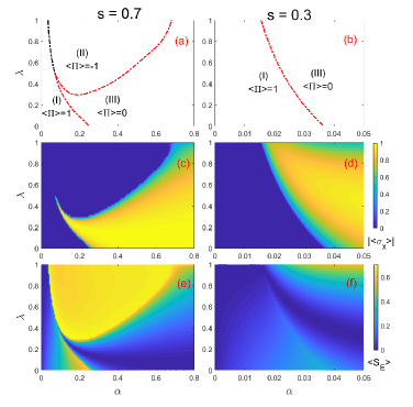
Figure 1: (Color online) (upper panel) Phase diagram in the $\alpha-\lambda$ plane for the ASBM drawn from the Parity $\left\langle\Pi\right\rangle$: delocalized phases with even (I) and odd parity (II) with conserved $Z_{2}$ symmetry, and the localized phase (III) with broken $Z_{2}$ symmetry. (middle panel) Order parameter $\left|\left\langle\sigma_{x}\right\rangle\right|$. (lower panel) Entanglement entropy $\left\langle S_{E}\right\rangle$. The power of the spectral function is (left) $s=0.7$ and (right) $0.3$. $\Delta=0.1$, $\omega_{c}=1$. The parameters used in the VMPS approach are $\Lambda=2$, $L=50$, $d_{opt}=12$, and $D=20,40$ for $s=0.3,0.7$, respectively.

Generally, the isotropic subohmic SBM exhibits the mean-field critical behavior for small $s$, and the nonclassical one for large $s$, so we focus on two typical powers of the spectral function $s=0.7$ and $0.3$ in this paper. The main results for the ASBM based on VMPS approaches are presented in Fig. 1 at $s=0.7$ (left) and $0.3$ (right). The different phases in the ASBM can be precisely characterized by the parity, which allows for composing the ground-state phase diagrams in the anisotropy $\lambda$ and the coupling strength $\alpha$ plane in the upper panel. We call phases I and II the two delocalized ones with $\left\langle\Pi\right\rangle=\pm 1$, respectively, and phase III as the localized phase with $\left\langle\Pi\right\rangle=0$. The boundary between the phase I and II is marked with the black dashed line, and the boundary of the phase III and any delocalized phases is indicated with the red dashed line. Clearly for $s=0.7$, we do observe three phases full with the phase diagram and a QuTP is the intersecting point of the three critical lines.

Color plots for the order parameter $\left|\left\langle\sigma_{x}\right\rangle\right|$ and the entanglement entropy $S_{E}$ between the two-level system and the environment bath are displayed in the middle and lower panels of Fig. 1, respectively. It is remarkable to see that the skeleton of the phase diagram can be directly obtained from the color plot of the entropy. In the small $\alpha$ region, the entropy increases quickly but still continuously within the phase I area, and no phase transition takes place. The order parameter share the common shape with the phase boundary marked by the red dashed line.

For small power of the spectral function, as shown in Fig. 1 (b) for $s=0.3$ that the phase diagram only consists of two phases (I and III). It follows that only a single 2nd-order QPT from the delocalized to localized phase is observed in this case, similar to the isotropic SBM. This phase diagram can be replotted in a similar way as Fig. 2 in Ref.  ciute for the anisotropic Dicke model, if using $\Omega_{E}\propto\sqrt{\alpha},\Omega_{M}\propto\lambda\sqrt{\alpha}$.

Surprisingly, for large power $s=0.7$, a new delocalized phase with odd parity (phase II) can grow at the phase III region and have a common border with phase I, as exhibited in Fig. 1 (a). It intervenes between phases I and III in an unusually way. The QPT between the two delocalized phases is of 1st-order due to the level crossing caused by the different wavefunctions with opposite parities, whereas the QPTs from any delocalized phase to localized phase are definitely of the 2nd-order due to the symmetry breaking.

For the highly anisotropic case, both the 1st- and 2nd-order QPTs take place successively from phases I to II, then to phase III, similar to the SBM in the RWA. Note however that the total excitation in the ASBM is not conserved, unlike the SBM in the RWA. Especially in the moderate anisotropic model, with increasing coupling strength, the system would undergo the 2nd-order QPTs for three times: ${I}\rightarrow III$, ${III}\rightarrow II$, and $I{I}\rightarrow III$. This unusual reentrance to the same localized phase has never been reported previously in the light-matter interacting systems. For the low anisotropic case, since the rotating-wave terms and the counterrotating terms are comparable, it is not essentially different from the isotropic SBM, and thus exhibits the similar critical phenomenon.

To be more complete, we have performed extensive calculation based on VMPS for many different values of $s$, and found that phase II only emerges for $s>0.38$ in the ASBM. We also extend the anisotropic constant regime to $\lambda>1$. In this case, we can absorb $\lambda$ into $g_{k}$, and have $g_{k}^{\prime}=\lambda g_{k}$. The coupling strength in Eq. (2) becomes $\alpha^{\prime}=\lambda^{2}\alpha$. Set $\lambda^{\prime}=1/\lambda$. The transformed Hamiltonian is the same as Hamiltonian (1) if interchanging the coefficients of the last two terms and removing primes in $\lambda^{\prime}$ and $\alpha^{\prime}$. Regarding $\left|\left\langle\sigma_{y}\right\rangle\right|$ as the order parameter, the phase diagram can be also obtained in the $\alpha^{\prime}-\lambda^{\prime}$ plane for $0<\lambda^{\prime}<1$, which is exactly the same as Fig. 1 for the same $s$. The results for $\lambda>1$ are qualitatively the same as those for the anisotropic parameter $1/\lambda$ at the same power $s$, because only the phase boundaries are scaled by $1/\lambda^{2}$ .

To study the QPTs deeply, we will discuss the order parameter and the entanglement entropy in detail in the next subsections. For more clarity, we extract the data of the parity, magnetization, and the entropy as a function of coupling strength $\alpha$ at $\lambda=0.3$ and $0.9$ in Fig. 1, and re-plot them in Fig. 2 for $s=0.7$ and Fig. 3 for $s=0.3$, respectively.

III.2 Order parameter

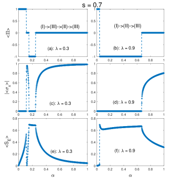
Figure 2: (Color online) Parity $\left\langle\Pi\right\rangle$ (upper panels), magnetization $\left|\left\langle\sigma_{x}\right\rangle\right|$ (middle panels), and entanglement entropy $\left\langle S_{E}\right\rangle$ (lower panels) as a function of $\alpha$ in the ground state for $\lambda=0.3$ (left) and $\lambda=0.9$ (right) by VMPS approach. $\Delta=0.1$, $\omega_{c}=1$, $\epsilon=0$, $\Lambda=2$, $L=50$, $d_{opt}=12$, and $D=40$ for $s=0.7$.

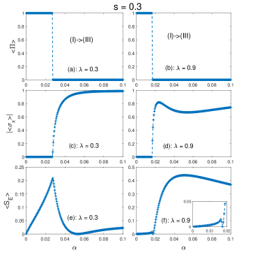
Figure 3: (Color online) Parity $\left\langle\Pi\right\rangle$ (upper panels), magnetization $\left|\left\langle\sigma_{x}\right\rangle\right|$ (middle panels), and entanglement entropy $\left\langle S_{E}\right\rangle$ (lower panels) as a function of $\alpha$ in the ground state for $\lambda=0.3$ (left) and $\lambda=0.9$ (right) by VMPS approach. $\Delta=0.1$, $\omega_{c}=1$, $\epsilon=0$, $\Lambda=2$, $L=50$, $d_{opt}=12$, and $D=20$ for $s=0.3$.

Generally, in the delocalized phase, spin has equal probability in the two states, spin-up and spin-down (both in $x$-axis here), while in localized phase, spin prefers to stay in one of the two states. Because phases I and II are delocalized ones with opposite parities ($\pm 1$), the order parameter must be zero due to the conserved symmetry. So we cannot distinguish phase II from phase I by the order parameter, which is shown in the blue regime of Fig. 1 (c). Nonzero order parameter is only found in the localized phase due to symmetry breaking. Thus, $\left|\left\langle\sigma_{x}\right\rangle\right|$, the order parameter, can only be used to determine the boundary of the continuous QPTs. The parity always jumps to different plateaus when crossing any phase boundaries. These characteristics are clearly shown in the upper panels of Figs. 2 and 3, which can be used to compose the phase diagram precisely.

One can indeed see that the order parameter remains zero in phases I and II and only becomes nonzero in the phase III in the middle panels of Figs. 2 and 3. The remarkable peak of the order parameter in Fig. 2 (c) for $s=0.7,\lambda=0.3$ is originated from the narrow localized phase III.

For small power of the spectral function,  say $s=0.3$, there only exist two phases: delocalized phase with even parity I and localized phase III. Although the phase II does not show up in the phase diagram in this case, it still plays some roles. The magnetization for different anisotropy shows different behaviors after the critical point in the middle panel of Fig. 3 for $\lambda=0.3$ and $\ 0.9$. For $\lambda=0.3$, the order parameter increases monotonously to the global maximum, while for $\lambda=0.9$, it displays a nonmountainous behavior with $\alpha$. One can find in the phase diagram that the high anisotropy $\lambda$ and large $s$ favor for the emergence of phase II. Even for small $s$, phase II finally disappears due to the failure in the competition with phase III, but its effect would not disappear completely without a trace. According to the different symmetry, it is to note that phase III enhances but phase II suppresses the magnetization, which cooperate to result in the local minimum of the magnetization in this region. Of course, if phase II somehow truly appears in this region, the magnetization must be zero, no local minimum can be seen.

III.3 Entanglement Entropy

The entanglement entropy $S_{E}$ is presented in the lower panel of Fig. 1 for $s=0.7$ and $0.3$. From the low panels of Figs. 2 and 3, we can observe that the entropy changes drastically when crossing all 1st- and 2nd-order critical lines. As shown in Ref. gu2004 in the fermionic systems, the entanglement can be used to identify QPTs.  So, the implications between the entanglement and the quantum phase in the present ASBM should also be nontrivial.

To shed some insights, we first consider the 1st-order QPT in the SBM in the RWA ($\lambda=1$) wangyz . In this case, the total excitation $\hat{N}=\sum_{k}a_{k}^{{\dagger}}a_{k}+\sigma_{+}\sigma_{-}$ is the conserved number. At the weak coupling, $\left\langle N\right\rangle=0$, corresponding to even parity $\left\langle\Pi\right\rangle=1$, the ground state wave-function is $\left|\psi_{0}\right\rangle=\left|0\right\rangle\left|\downarrow\right\rangle$ with energy $E_{0}=-\frac{\Delta}{2}$, then we can obtain the reduced density matrix for the spin

$$\rho_{spin}=\left|\downarrow\right\rangle\left\langle\downarrow\right|,$$

and one can easily obtained entropy $S_{E}=0$ from Eq. (9).

When exceeding the 1st QPT point, $\left\langle N\right\rangle$ jumps to $1$ corresponding to odd parity $\left\langle\Pi\right\rangle=-1$, the ground state wave-function for the single excitation is

$$\left|\psi_{1}\right\rangle=c\left|0\right\rangle\left|\uparrow\right\rangle+\sum_{k}d_{k}{a_{k}}^{{\dagger}}\left|0\right\rangle\left|\downarrow\right\rangle,$$ (10)

where $c$ and $d_{k}$ are the coefficients for the bosonic vacuum and single boson number states. On can easily obtain $c^{2}=\left(1+\left\langle\sigma_{z}\right\rangle\right)/2$. The reduced density matrix for the spin is

$$\rho_{spin}=c^{2}\left|\uparrow\right\rangle\left\langle\uparrow\right|+\left(1-c^{2}\right)\left|\downarrow\right\rangle\left\langle\downarrow\right|.$$ (11)

If $\left\langle\sigma_{z}\right\rangle=0$, we obtain the maximum entropy $S_{E}^{\max}=\log 2=0.693$ from Eq. (9). In this case, the probabilities of spin-up and spin-down are equal, corresponding to the largest entanglement between spin and bath. In the single excitation state $\left\langle\sigma_{z}\right\rangle$ is usually small. e.g. it is found in Fig. 2(b) of our previous work wangyz that  $\left\langle\sigma_{z}\right\rangle$ suddenly switches to a small value around $0.3\pm 0.1$ when crossing the 1st-order QPT point. The entropy in the single excitation state can be larger than $0.6$.

In the presence of the counter rotating wave terms in the ASBM, the total excitation $\hat{N}$ is no longer conserved. The state with the even parity at the weak coupling is not $\left|\psi_{0}\right\rangle=\left|0\right\rangle\left|\downarrow\right\rangle$ any more, the components with the even number $\hat{N}$ excitations in the states would be involved gradually with the increase of the coupling strength, so the entropy increases within phase I, consistent with the numerical calculations shown in the lower panels of Figs. 2 and 3.

Because phase II is of odd parity, as long as $\lambda\neq 1$, its state is different from but close to the state (10) with a single excitation. So the entropy is also high in phase II. We indeed find that the entropy in all phase II regime is high, indicating it is a highly entangled phase. As shown in Fig. 1 (e), a highly entanglement regime appears in the phase II area. In the 1st-order QPT boundary from phases I and II, the entropy jumps suddenly to a value close to  $S_{E}^{\max}$ in phase II, as is just shown in Fig. 2 (f) at $s=0.7,\lambda=0.9$.

In the localized phase of the isotropic SBM, Chin et al. found a monotonic decrease of entanglement above the transition by means of the nonadiabatic modes Chin analytically, consistent with the numerical calculations lehur . In the present ASBM, this behavior may be modified due to the competition between the localized phase III and the hidden phase II, the latter is lacking in the isotropic SBM but still possibly present in the ASBM under some condition. In the phase III region of the lower panel of Fig. 3 for $s=0.3$, at $\lambda=0.3$ and $0.9$, we note that the entropy decreases first, reaches a local minimum, and surprisingly rises again when the coupling strength increases further, in contrast to the isotropic SBM. As discussed in the last subsection, the phase III competes with phase II in this area and wins finally. In general, phase III exhibits a finite value of order parameter but weak entanglement between spin and bosonic bath, while phase II displays high entanglement but suppresses the order parameter completely. Although phase II cannot appear finally, it could still be hidden there and enhance the entanglement. The observed local minimum is just caused by the cooperated effect of the competition of phases II and III beyond the weak coupling. We have confirmed that, in the strong coupling limit, the entropy in all cases must vanish (not shown here).

III.4 Evidence for 1st-order QPT between the phases with opposite parities by MCS variational studies

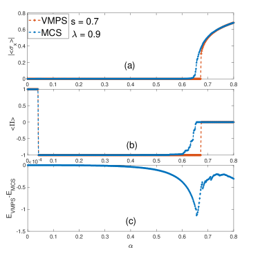
Figure 4: (Color online) (a) The order parameter $\left|\left\langle\sigma_{x}\right\rangle\right|$, (b) the parity $\left\langle\Pi\right\rangle$ as a function of the coupling strength within VMPS and MCS variational approaches. (c) The difference between the VMPS ground-state energy and that by MCS. $s=0.7$, $\lambda=0.9$, $\Delta=0.1$, $\omega_{c}=1$, $\epsilon=0$, $\Lambda=2$, $L=20$, $d_{opt}=12$, $D=20$, $N_{c}=9$.

The most interesting observation in the ASBM is that a new phase II with odd parity intervenes between the conventional phase I and III, which is absent in the isotropic SBM.  To provide more evidence of this new quantum phase, we also employ the MCS approach here.  By VMPS, for $s=0.7$ and $\lambda=0.9$, we have observed that a large region of phase II appears between phases I and III. Since all the three phases can be described well in the trial wave function (7), we in principle can detect these phases in the MCS framework. In Fig. 4, we list results for the parity, the magnetization, and the ground-state energy by both MCS and VMPS approaches for $s=0.7$ and $\lambda=0.9$. Notice that only $L=20$ bosonic modes are taken for both approaches here due to the computational difficulties in the MCS approach. However, it does not influence the essential results at all. The results in the large part of the phase II regime by both approaches are almost the same, convincingly demonstrating the existence of the phase II according to its characteristics. The wavefunction in the MCS reproduces the phase II with the odd parity explicitly by noting $A_{n}=-{B_{n}}$. The deviation of the results in the transition regime between phases II and III is indeed visible, but it does not influence the existence of phase II. We should point out that the MCS approach is used here to provide another piece of evidence for the existence of phase II qualitatively, not for the precise location of the critical points.

III.5 The critical exponent for the order parameters

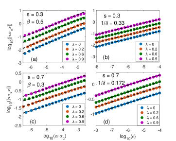
Figure 5: (Color online) The log-log plot of the magnetization $\left|\left\langle\sigma_{x}\right\rangle\right|$ as a function of $\alpha-\alpha_{c}$ (left) at $\epsilon=0$ and bias $\epsilon$ (right) at $\alpha=\alpha_{c}$ of the ASBM for $s=0.3$ (upper panel) and $s=0.7$ (lower panel). The numerical results by VMPS are denoted by blue, orange, green, purple circles for $\lambda=0,0.2,0.6,0.9$ respectively, and the power-law fitting curves are denoted by the black dashed lines, which shows $\beta=0.5,0.3$ and $1/\delta=0.33,0.172$ for $s=0.3,0.7$ respectively. For visibility, the curves for different $\lambda$ have been shifted to distinguish them. $\Delta=0.1$,$\omega_{c}=1$, $\Lambda=2$, $L=50$, $d_{opt}=12$, and $D=20,40$ for $s=0.3,0.7$ respectively.

The critical behavior of the 2nd-order QPT from phase I to III and from phases II to III are discussed in this subsection.  We present the log-log plot of the order parameter $\left|\left\langle\sigma_{x}\right\rangle\right|$ as a function of $\alpha-\alpha_{c}$ at $\epsilon=0$ and as a function of the bias $\epsilon$ at $\alpha=\alpha_{c}$ for $s=0.3$ and $s=0.7$ with different anisotropic parameters $\lambda=0,0.2,0.6,0.9$ in the critical regime in Fig. 5. The order parameter critical exponents $\beta$ and $\delta$ can be determined by fitting power-law behavior, $\left|{\left\langle{\sigma_{x}}\right\rangle}\right|\propto{\left({\alpha-{\alpha_{c}}}\right)^{\beta}}$ with the bias $\epsilon=0$ and $\left|{\left\langle{\sigma_{x}}\right\rangle}\right|\propto\epsilon^{1/\delta}$ at $\alpha=\alpha_{c}$. All the critical exponents of the anisotropic model show the same rules as the isotropic SBM. It takes the mean-field value $\beta=1/2,1/\delta=1/3$ for $s<1/2$ and the hyperscaling $\beta<1/2,1/\delta=\left(1-s\right)/\left(1+s\right)$ for $s>1/2$.

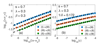
Figure 6: (Color online) The log-log plot of the magnetization $\left|\left\langle\sigma_{x}\right\rangle\right|$ as a function of $\left|\alpha-\alpha_{c}\right|$ (left) at $\epsilon=0$ and bias $\epsilon$ (right) at $\alpha=\alpha_{c}$ of the ASBM for $s=0.7,\lambda=0.3$. The numerical results by VMPS are denoted by blue, orange, green, circles for the critical processes (I) to (III), (III) to (II) and (II) to (III) respectively, and the power-law fitting curves are denoted by the black dashed lines, which shows $\beta=0.3$ (left) and $1/\delta=0.172$ (right) for $0.7$ respectively. For visibility, the curves for different $\lambda$ have been shifted to distinguish them. $\Delta=0.1$,$\omega_{c}=1$, $\Lambda=2$, $L=50$, $d_{opt}=12$, and $D=40$ for $s=0.7$ respectively.

In the present subohmic ASBM, there is at least one 2nd-order QPT from the conserved parity phase to the phase III. For large $s$ and the moderate anisotropy, the model even experiences several 2nd-order QPTs with the increase of the coupling strength. We also evaluate the critical exponents for these multiple 2nd-order QPTs for $s=0.7,\lambda=0.3$ in Fig. 6. Very surprisingly, the same critical exponents $\beta$ and $\delta$ are obtained, indicating that they belong to the same universality class. Based on these observations, we can say that, counterrotating terms would almost have no effect on critical exponents even when several 2nd-order QPTs are present successively at a few critical points for fixed anisotropy in the ASBM.

The universality in the QuTP in the ASBM is a very challenging issue. According to the Landau theory, it should be different from those in other critical points. The numerical calculations cannot be used to isolate the QuTP from other critical points, and much less distinguish the universality. The analytical treatment is, however, lacking in any SBMs except in the ohmic bath, unlike the Dicke models Dicke ; ciute ; puhan . A field theory formulated from the Feynman path-integral representation of the partition function for the SBM Leggett ; map ; berry ; Kirchner might be extended to the ASBM. Then analytical arguments based on the quantum-to-classical mapping would be helpful to clarify this issue.

IV Conclusion

We have found rich quantum phases in the ASBM with the subohmic bath by the VMPS approach. The phase diagram has been composed in the coupling strength and anisotropy space.  For large powers of the spectral function, two 2nd-order QPT critical lines meet the 1st-order QPT line at the same point, which is just a QuTP. At any 2nd-order QPT lines, the critical exponent of the order parameter and its field related critical exponents are the same, which only depend on the power of the spectral function. All phase boundaries can be precisely determined by the parity and the entanglement entropy, besides, the 2nd-order QPTs can also be detected by the magnetization. The 1st-order QPTs between opposite parity symmetry have been corroborated by the MCS approach where we can directly observe opposite parity in the ground-state wavefunction. For low powers of the spectral function, the system only experiences the 2nd-order QPT from the delocalized to localized phases, similar to the isotropic SBM.

The newly found symmetric quantum phase with odd parity emerges for large power of the spectra function at the highly anisotropic case and borders to the conventional symmetric phase with even parity, which enriches the critical phenomena in the spin and boson coupling systems. Although this phase shares the same odd parity with the phase in the single excitation in the SBM under the RWA, the total excitation number is not conserved. The QPT to the localized phase from a delocalized one with odd parity has never been found before in the spin and boson coupling systems. The ASBM might be realized in the superconducting circuit QED system where the anisotropic parameters can be manipulated artificially. We believe that the ASBM would serve as a new important lab to study the rich quantum criticality.

ACKNOWLEDGEMENTS This work is supported by the National Science Foundation of China (Nos. 11834005, 11674285), the National Key Research and Development Program of China (No. 2017YFA0303002),

^∗ Email:qhchen@zju.edu.cn

References

- (1) S. Sachdev, Quantum Phase Transitions, 2nd ed. (Cambridge University Press, Cambridge, England, 2011).
- (2) V. J. Emery in Highly Conducting One-Dimensional Solids edited by J. T. Devreese, R. P. Evrard and V. E. van Doren (Plenum, New York, 1979), pp. 247 C303; H.-Q. Lin, E. R. Gagliano, D. K. Campbell, E. H. Fradkin and J. F. Gubernatis, in The Hubbard Model: Its Physics and Mathematical Physics edited by D. Baeriswyl, D. K. Campbell, J. M. P. Carmelo, F. Guinea and E. Louis (Springer, New York, 1995), pp. 315 C327.
- (3) M. Greiner, O. Mandel, T. Esslinger, T. W. HaEnsch, and I. Bloch, Nature(London) 415, 39 (2002).
- (4) E. Fradkin and J. E. Hirsch, Phys. Rev. B 27, 1680 (1983); W.-Q. Ning, H. Zhao, C.-Q. Wu, and H.-Q. Lin, Phys. Rev. Lett. 96, 156402 (2006); E. A. Nowadnick, S. Johnston, B. Moritz, R. T. Scalettar, and T. P. Devereaux, Phys. Rev. Lett. 109, 246404 (2012).
- (5) A. J. Leggett, S. Chakravarty, A. T. Dorsey, M. P. A. Fisher, A. Garg, and W. Zwerger, Rev. Mod. Phys. 59, 1(1987).
- (6) M.-J. Hwang, R. Puebla, and M. B. Plenio, Phys. Rev. Lett.115, 180404 (2015); M. X. Liu, S. Chesi, Z.-J. Ying, X. S. Chen, H.-G. Luo, H.-Q. Lin, Phys. Rev. Lett. 119, 220601 (2017).
- (7) R. H. Dicke, Phys. Rev. 93, 99 (1954); C. Emary and T. Brandes, Phys. Rev. E 67, 066203 (2003) ; Phys. Rev. Lett. 90, 044101 (2003); Q.-H. Chen, Y.-Y. Zhang, T. Liu, and K.-L. Wang, Phys. Rev. A 78, 051801 R (2008); T. Liu, Y.-Y. Zhang, Q.-H. Chen, and K.-L. Wang, Phys. Rev. A 80, 023810(2009).
- (8) R. Bulla, N. Tong, and M. Vojta, Phys. Rev. Lett. 91, 170601 (2003); M. Vojta, N. Tong, and R. Bulla, Phys. Rev. Lett. 94, 070604 (2005); R. Bulla, Phys. Rev. Lett.102, 249904(E) (2009).
- (9) Q. Si, S. Rabello, K. Ingersent, and J. L. Smith, Nature (London) 413, 804 (2001) and Phys. Rev. B 68, 115103 (2003).
- (10) J. Ye and C. L. Zhang, Phys. Rev. A 84, 023840 (2011).
- (11) A. Baksic and C. Ciuti, Phys. Rev. Lett. 112, 173601 (2014).
- (12) Z. Q. Zhang, C. H. Lee, R. Kumar, K. J. Arnold, S. J. Masson, A. L. Grimsmo, A. S. Parkins, and M. D. Barrett, Phys. Rev. A 97 043858 (2018).
- (13) Y. Xu and H. Pu, Phys. Rev. Lett. 122, 193201 (2019).
- (14) R. B. Griffiths, Phys. Rev. Lett. 24, 715 (1970).
- (15) M. O. Scully and M. S. Zubairy, Quantum Optics (Cambridge University Press, Cambridge, 1997).
- (16) H. P. Breuer and F. Petruccione, The Theory of Open Quantum Systems (Oxford University Press, New York, 2002).
- (17) U. Weiss, Quantum Dissipative Systems (World Scientific, Singapore, 2008).
- (18) T. Niemczyk et al., Nature Physics 6, 772 (2010).
- (19) F. Yoshihara, T. Fuse, S. Ashhab, K. Kakuyanagi, S. Saito, and K. Semba, Nat. Phys. 13, 44 (2017).
- (20) F. Dimer, B. Estienne, A. S. Parkins, and H. J. Carmichael, Phys. Rev. A 75, 013804 (2007); K. Baumann, C. Guerlin, F. Brennecke, and T. Esslinger, Nature (London) 464, 1301 (2010).
- (21) J. I. Cirac, A. S. Parkins, R. Blatt, and P. Zoller, Phys. Rev. Lett. 70, 556 (1993).
- (22) P. Forn-Díaz, J. J. García-Ripoll, B. Peropadre, J.-L. Orgiazzi, M. A. Yurtalan, R. Belyansky, C. M. Wilson, and A. Lupascu, Nat. Phys. 13, 39 (2017).
- (23) J. Keeling, M. J. Bhaseen, and B. D. Simons, Phys. Rev. Lett. 105, 043001 (2010).
- (24) Q. T. Xie, S. Cui, J. P. Cao, L. Amico, and H. Fan, Phys. Rev. X 4, 021046 (2014).
- (25) A. L. Grimsmo and S. Parkins, Phys. Rev. A 87 033814 (2013).
- (26) A. Winter, H. Rieger, M. Vojta, and R. Bulla, Phys. Rev. Lett. 102, 030601 (2009).
- (27) A. Alvermann and H. Fehske, Phys. Rev. Lett. 102, 150601 (2009).
- (28) M. Vojta, R. Bulla, F. Güttge, and F. Anders, Phys. Rev. B 81, 075122 (2010).
- (29) Y.-Y. Zhang, Q.-H. Chen, and K.-L. Wang, Phys. Rev. B 81, 121105(R)(2010).
- (30) A. W. Chin, J. Prior, S. F. Huelga and M. B. Plenio, Phys. Rev. Lett. 107, 160601 (2011).
- (31) C. Guo, A. Weichselbaum, J. von Delft, and M. Vojta, Phys. Rev. Lett. 108, 160401 (2012).
- (32) M. F. Frenzel and M. B. Plenio, New Journal of Physics 15, 073046(2013).
- (33) C. R. Duan, Z. F. Tang, J. S. Cao, and J. L. Wu, Phys. Rev. B 95, 214308 (2017).
- (34) S. He, Li. W. Duan, and Q. -H. Chen, Phys. Rev. B 97, 115157 (2018).
- (35) Y.-Z. Wang, S He, L.-W. Duan, Q.-H. Chen. Phys. Rev. B 100, 115106 (2019).
- (36) A. W. Chin, A. Rivas, S. F. Huelga, and M. B. Plenio, Journal of Mathematical Physics 51, 092109 (2010).
- (37) F. A. Y. N. Schrder, A. W. Chin, Phys. Rev. B 93, 075105 (2016).
- (38) A. Weichselbaum, F. Verstraete, U. Schollwck, J. I. Cirac, and J. von Delft, Phys. Rev. B 80, 165117 (2009).
- (39) H. Saberi, A. Weichselbaum, and J. von Delft, Phys. Rev. B 78, 035124 (2008).
- (40) Q. B. Ren and Q. H. Chen, Chin. Phys. Lett. 22, 2914 (2005).
- (41) S. Bera, S. Florens, H. U. Baranger, N. Roch, A. Nazir, A. W. Chin, Phys. Rev. B 89, 121108(R) (2014); S. Bera, A. Nazir, A. W. Chin, H. U. Baranger, S. Florens, Phys. Rev. B 90, 075110 (2014).
- (42) L. Duan, S. He, Q.-H. Chen, arXiv:1412.6343.
- (43) Z. Blunden-Codd, S. Bera, B. Bruognolo, N.-O. Linden, A. W. Chin, J. von Delft, A. Nazir, and S. Florens, Phys. Rev. B 95, 085104 (2017).
- (44) S. -J. Gu, S. -S. Deng, Y. -Q. Li, and H. -Q. Lin, Phys. Rev. Lett. 93, 086402 (2004).
- (45) K. Le Hur, P. Doucet-Beaupre and W. Hofstetter, Phys. Rev. Lett. 99, 126801 (2007).
- (46) M. Vojta, Phys. Rev. B 85, 115113 (2012)
- (47) S. Kirchner, J. Low Temp. Phys. 161, 282 (2010).
- (48) S. Kirchner, Q. Si, and K. Ingersent, Phys. Rev. Lett. 102, 166405 (2009); S. Kirchner, K. Ingersent, and Q. Si, Phys. Rev. B. 85, 075113(2012).