Correlating nonlinear time series and spectral properties of IGR J17091-3624: Is it similar to GRS 1915+105?

Abstract

We explore the nonlinear properties of IGR J17091-3624 in the line of the underlying behaviour for GRS 1915+105, following correlation integral method. We find that while the latter is known to reveal the combination of fractal (or even chaotic) and stochastic behaviours depending on its temporal class, the former mostly shows stochastic behaviour. Therefore, although several observations argue IGR J17091-3624 to be similar to GRS 1915+105 with common temporal classes between them, underlying nonlinear time series analyses offer differently. Nevertheless, the Poisson noise to $rms$ variation value for IGR J17091-3624 turns out to be high, arguing them to be Poisson noise dominated and hence may plausibly lead to suppression of the nonlinear character, if any. Indeed, it is a very faint source compared to GRS 1915+105. However, by increasing time bin some of the temporal classes of IGR J17091-3624 show deviation from stochasticity, indicating plausibility of higher fractal dimension. Along with spectral analysis, overall IGR J17091-3624 argues to reveal three different accretion classes: slim, Keplerian and advective accretion discs.

1 Introduction

On timescales of seconds to minutes, the three sources, GRS 1915+105, IGR J17091-3624 and MXB 1730-335, have been shown to exhibit a variety of peculiar variability properties in their lightcurves not normally seen in other low mass X-ray binaries (LMXBs). In the black hole X-ray binaries (BHXBs) GRS 1915+105 and IGR J17091-3624, these properties are categorized into variability classes. While most LMXBs transit between quiescence and outbursts (including IGR J17091-3624), GRS 1915+105 has been in outburst since it was discovered in 1992 (Castro-Tirado et al., 1992).

IGR J17091-3624, on the other hand, is an LMXB discovered during an outburst by INTEGRAL in 2003 (Kuulkers et al., 2003). It again went into outburst in 2011 (Krimm & Kennea, 2011) and was observed by RXTE, Swift, XMM-Newton, Chandra and Suzaku and most recently in 2016 (Miller et al. 2016; Grinberg et al. 2016). During the long duration of the $2011$ outburst, analyses of the lightcurves show GRS 1915+105 like properties in several of the individual observations (Altamirano et al., 2011; Altamirano & Belloni, 2012; Pahari et al., 2014; Court et al., 2017). While GRS 1915+105 reveals 12 distinct temporal classes (Belloni et al., 2000), IGR J17091-3624 is also found to exhibit 9 temporal classes (Altamirano et al., 2011; Court et al., 2017). Nevertheless, at $2-25\,\mathrm{keV}$, IGR J17091-3624 is about a factor of 20 fainter than GRS 1915+105 implying plausibly that IGR J17091-3624 is at a larger distance, and/or hosts a smaller black hole or has a lower accretion rate $\dot{m}$ than GRS 1915+105.

The time series of GRS 1915+105 was repeatedly found to exhibit, sometimes fractal (or even chaotic) and sometimes stochastic behaviours (Misra et al., 2004; Mukhopadhyay, 2004; Misra et al., 2006) based on the correlation integral (CI) calculation, depending on its temporal class (Belloni et al., 2000). In an attempt to understanding the bursting behaviour seen in GRS 1915+105, Massaro et al. (2014) and Ardito et al. (2017) considered a simple mathematical framework composed of nonlinear differential equations. They concluded from their modelling that the complex behaviour seen in the source may be regulated mainly by a single nonlinear oscillator that is driven by a unique parameter – plausibly the outer mass accretion rate – whose changes may be responsible for the variability classes. Recently, based on correlating temporal (time series) and spectral properties, the source has been argued to exhibit different accretion classes: advection dominated accretion (Narayan & Yi, 1994), general advective accretion (Rajesh & Mukhopadhyay, 2010), Keplerian accretion disc (Shakura & Sunyaev, 1973), and slim disc (Abramowicz et al., 1988) flows, switching from one to another with time (Adegoke et al., 2018). As IGR J17091-3624 has already been found to have similarities in several observations with GRS 1915+105, naturally the question arises if it also exhibits the combination of fractal/chaotic and stochastic natures in classes and also similar temporal and spectral correlations arguing for 4 accretion classes, as found in GRS 1915+105? This we plan to explore here.

The plan of the paper is the following. In the next section, we give an overview of the CI method. We discuss the observed data under consideration from three satellites in §3. Subsequently, we explain various results by analyzing data in §4. Significance of observed stochasticity in order to conclude from such analyses is discussed in §5. Finally we end with a conclusion along with discussions in §6.

2 Correlation Integral method

The delay embedding technique of Grassberger & Procaccia (1983) is one of the standard methods used to reconstruct the dynamics of a nonlinear system from a time series. The detailed technique in the astrophysical context was already discussed earlier (Karak et al. 2010), here we briefly recall them for completeness. It requires constructing a CI defined as the probability that two points in phase space are closer together than a distance $r$. It is normally required that the dynamics be constructed for different embedding dimensions $M$, since the number of equations or variables describing the system is not known a priori. In using this method, vectors of length $M$ are created from the time series $y(t_{i})$ using a delay time $\tau$ such that

$$X(t_{i})=(y(t_{i}),y(t_{i}+\tau),y(t_{i}+2\tau),...,y(t_{i}+(M-1)\tau))$$ (1)

for the $i$-th vector.

As a condition, the times $t_{i}$ should be evenly spaced and should be chosen such that the number of data points is sufficiently large. More so, the choice of $\tau$ should be such that any two components of vectors are not correlated.

The quantity $D_{2}$ known as correlation dimension provides a quantitative picture of this technique. Computationally, it involves choosing a large number of points in the reconstructed dynamics as centres and then computing CI $C_{M}(r)$, which is the number of points that are within a distance $r$ from the centre averaged over all the centres, written as

$$C_{M}(r)=\frac{1}{N({N_{c}-1})}\mathop{\sum^{N}\sum^{N_{c}}}_{i=1\ j\neq i\ j=1}{H(r-|{x_{i}-x_{j}}|)},$$ (2)

where $N$ and $N_{c}$ are the number of points and the number of centres respectively, $x_{i}$ and $x_{j}$ are the reconstructed vectors and $H$ is the Heaviside step function.

The correlation dimension $D_{2}$ being just a scaling index of the variation of $C_{M}(r)$ with $r$ is expressed as

$$D_{2}=\mathop{\lim}\limits_{r\to 0}\left(\frac{d\rm{log}C_{M}(r)}{d\rm{logr}}\right).$$ (3)

The effective number of differential equations governing the dynamics of the system can be inferred from the value of $D_{2}$ in principle. The linear part of the plot of $\rm{log}[C_{M}(r)]$ against $\rm{log}[r]$ can be used to estimate $D_{2}$. The nonlinear dynamical properties of the system is revealed from the variation of $D_{2}$ with $M$. If for all $M$, $D_{2}\approx M$ then the system is stochastic. On the other hand, the system is deterministic if initially $D_{2}$ increases linearly with $M$ until it reaches a certain value and saturates. This saturated value of $D_{2}$ is then taken to be the fractal/correlation dimension of the system, plausibly a signature of chaos (subject to the confirmation by other methods). While the saturated $D_{2}$ (i.e. $D_{2}^{sat}$) gives a quantitative measure of the dynamics, the corresponding critical dimension $M_{cr}$ is a measure of the number of equations required to describe the behaviour of the system.

Table 1: IGR J17091-3624: Basic flow classes

ObsID	class	GRS 1915-like class	behaviour	diskbb	PL	GA	SI	$\chi^{2}/dof$	state	diskbb $T_{in}$	$F\,\times 10^{-10}$
96420-01-01-00	I	$\chi$	S	$10.0$	$89.1$	$0.9$	$2.26^{+0.02}_{-0.02}$	$1.12\,(48/43)$	PD	$1.11\pm{0.05}$	$11.949$
96420-01-11-00	II	$\phi$	S	$18.5$	$81.5$	$-$	$2.33^{+0.04}_{-0.04}$	$1.04\,(47/45)$	PD	$1.13\pm{0.02}$	$6.238$
96420-01-04-01	III	$\nu$	S	$38.0$	$62.0$	$-$	$2.25^{+0.07}_{-0.07}$	$0.82\,(37/45)$	PD	$1.20\pm{0.01}$	$9.730$
96420-01-05-00	IV	$\rho$	S	$41.6$	$58.0$	$0.4$	$2.34^{+0.05}_{-0.05}$	$1.06\,(45/43)$	PD	$1.20\pm{0.01}$	$9.676$
96420-01-06-03	V	$\mu$	S/NS	$54.4$	$45.6$	$-$	$2.55^{+0.07}_{-0.07}$	$1.28\,(58/45)$	D-P	$1.43\pm{0.01}$	$9.313$
96420-01-09-00	VI	$\lambda$	S	$65.8$	$34.2$	$-$	$2.55^{+0.09}_{-0.09}$	$1.37\,(61/45)$	DD	$1.85\pm{0.03}$	$10.099$
96420-01-18-05	VII	$none$	S	$63.4$	$36.6$	$-$	$2.61^{+0.15}_{-0.15}$	$0.65\,(29/45)$	DD	$1.50\pm{0.03}$	$8.603$
96420-01-19-03	VIII	$none$	S/NS	$73.4$	$26.4$	$0.2$	$2.29^{+0.12}_{-0.12}$	$1.30\,(56/43)$	DD	$1.78\pm{0.02}$	$10.596$
96420-01-35-02	IX	$\gamma$	S	$68.2$	$31.8$	$-$	$2.52^{+0.08}_{-0.08}$	$1.58\,(71/45)$	DD	$2.07\pm{0.03}$	$11.409$

Columns:- 1: RXTE observational identification number (ObsID). 2: Temporal class. 3: GRS 1915+105-like temporal class. 4: The behaviour of the system (F: low correlation/fractal dimension; S: Poisson noise like stochastic). 5: $\%$ of multi-colour blackbody component. 6: $\%$ of powerlaw component. 7: $\%$ Gaussian line component (XSPEC model gauss). 8: Powerlaw photon spectral index. 9: Reduced $\chi^{2}$. 10: Spectral state (DD: disc dominated; D-P: disc-powerlaw contributed; PD: powerlaw dominated). 11: diskbb temperature in units of $keV$. 12: Total flux in the $3-25$ keV in units of $erg\,cm^{-2}\,s^{-1}$

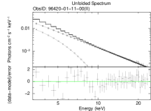
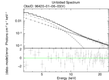
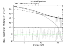
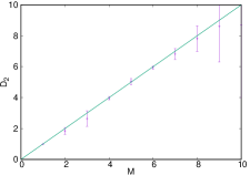
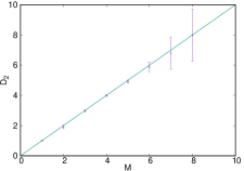
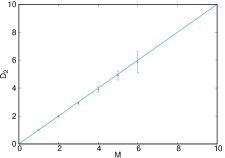
Figure 1: Top panels (left to right): Unfolded spectra for RXTE ObsIDs $96420-01-11-00$ (Class II), $96420-01-06-03$ (Class V) and $96420-01-18-05$ (Class VII) of IGR J17091-3624. The curves with square and circle symbols represent respectively diskbb and powerlaw contributions and the topmost solid curve in each panel represents the overall spectrum. Bottom panels (left to right): Variation of correlation dimension as a function of embedding dimension with errors for RXTE ObsIDs $96420-01-11-00$ (Class II), $96420-01-06-03$ (Class V) and $96420-01-18-05$ (Class VII) of IGR J17091-3624. The solid diagonal line in each panel represents the ideal stochastic curve. See Tables 1 and 4 for other details.

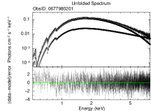
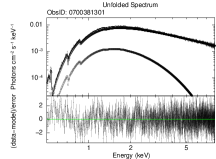
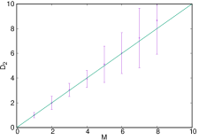
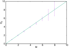
Figure 2: Top panels: Unfolded spectra for XMM-Newton ObsIDs 0677980201 (top-left) and 0700381301 (top-right) of IGR J17091-3624. The curves with square and circle symbols represent respectively diskbb and powerlaw contributions and the topmost solid curve in each panel represents the overall spectrum. Bottom panels: Variation of correlation dimension as a function of embedding dimension with errors for XMM-Newton ObsIDs 0677980201 (bottom-left) and 0700381301 (bottom-right) of IGR J17091-3624. The solid diagonal line in each panel represents the ideal stochastic curve.

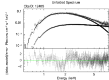
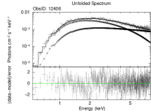
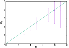
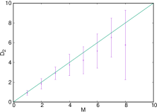
Figure 3: Top panels: Unfolded spectra for Chandra ObsIDs 12405 (top-left) and 12406 (top-right) of IGR J17091-3624. The curves with square and circle symbols represent respectively diskbb and powerlaw contributions and the topmost solid curve in each panel represents the overall spectrum. Bottom panels: Variation of correlation dimension as a function of embedding dimension with errors for Chandra ObsIDs 12405 (bottom-left) and 12406 (bottom-right) of IGR J17091-3624. The solid diagonal line in each panel represents the ideal stochastic curve.

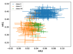
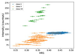
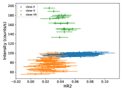
Figure 4: Left panel: Colour-Colour diagrams for classes II, V and VII of IGR J17091-3624 from RXTE, given in Table 1. Middle and Right panels: Hardness-Intensity diagrams for the same classes. See text for details.

Table 2: XMM-Newton observations

ObsID	IGR J17091 class	behaviour	diskbb	PL	GA	SI	$\chi^{2}/dof$	state	diskbb $T_{in}$	$F\,\times 10^{-10}$
0677980201	IV	S	$72.1$	$27.9$	$-$	$1.41^{+0.18}_{-0.18}$	$1.04$	DD	$1.16\pm{0.01}$	$17.562$
0700381301	After RXTE	S	$39.4$	$60.6$	$-$	$1.31^{+0.02}_{-0.02}$	$1.09$	PD	$0.73\pm{+0.04}$	$0.938$

Columns:- 1: Observational identification number. 2: IGR J17091-3624 temporal class. 3: The behaviour of the system (F: low correlation/fractal dimension. S: Poisson noise like stochastic). 4: $\%$ of multi-colour disc blackbody component. 5: $\%$ of powerlaw component. 6: $\%$ of Gaussian line component (XSPEC model gauss). 7. Powerlaw photon spectral index. 8: Reduced $\chi^{2}$. 9: Spectral state (DD: disc dominated; PD: powerlaw dominated). 10: diskbb temperature in units of $keV$. 11: Total flux in the $0.5-8$ keV in units of $erg\,cm^{-2}\,s^{-1}$.

Table 3: Chandra observations

ObsID	IGR J17091 class	behaviour	diskbb	PL	GA	SI	$\chi^{2}/dof$	state	diskbb $T_{in}$	$F\,\times 10^{-10}$
12405	VII	S	$63.8$	$31.7$	$-$	$0.51^{+0.95}_{-0.95}$	$1.318$	DD	$1.19^{+0.08}_{-0.08}$	$12.760$
12406	IX	S	$50.5$	$49.5$	$-$	$0.58^{+0.80}_{-0.80}$	$1.016$	PD	$1.53^{+0.15}_{-0.15}$	$1.220$

Columns:- 1: Observational identification number. 2: IGR J17091-3624 temporal class. 3: The behaviour of the system (F: low correlation/fractal dimension; S: Poisson noise like stochastic). 4: $\%$ of multi-colour disc blackbody component. 5: $\%$ of powerlaw component. 6: $\%$ of Gaussian line component (XSPEC model gauss). 7: Powerlaw photon spectral index. 8: Reduced $\chi^{2}$. 9: Spectral state (DD: disc dominated; PD: powerlaw dominated). 10: diskbb temperature in units of $keV$. 11: Total flux in the $0.5-8$ keV in units of $erg\,cm^{-2}\,s^{-1}$.

3 Observation and data reduction

The data we use in our analysis were obtained during the $2011-2013$ outburst of IGR J17091-3624 from RXTE, XMM-Newton and Chandra. To allow for easy and efficient cross verification, we use the same data reported by Court et al. (2017). In all cases, we use single orbit data for each observation ID (ObsID). This is to avoid the need to interpolate over data gaps that may result from merging observations across orbits, as this may adversely affect results from the CI method.

3.1 RXTE

We analyse data from the proportional counter array (PCA; Jahoda et al., 1996). We create background subtracted spectra and lightcurves following standard procedure on standard 2 and the science event data (Good Xenon). In Table 1, we show the list of ObsIDs that we use. We choose the energy range $3-25\,\mathrm{keV}$ for our RXTE spectral analysis. For our timing analysis, we bin the science event lightcurves to $0.125\,\mathrm{s}$, unless stated otherwise, and the standard 2 lightcurves to $32\,\mathrm{s}$. In order to probe the hardness variability using a model independent approach over the duration of the outburst, we further consider three energy bands: A($2-6\,\mathrm{keV}$), B($6-16\,\mathrm{keV}$) and C($16-60\,\mathrm{keV}$), using the $32\,\mathrm{s}$ binned standard 2 lightcurves.

3.2 XMM-Newton

We use two XMM-Newton observations of IGR J17091-3624 with ObsIDs $0677980201$ and $0700381301$ (given in Table 2) in our analysis. For both observations, we use EPIC-pn data obtained in timing mode and we generate lightcurves with a time bin of $5\,\mathrm{s}$. We employ the XMM-Newton Science Analysis System (SAS v.16.1.0) package for data reduction with updated Current Calibration Files (CCFs). We generate spectra and lightcurves from the product of the meta-task XMMEXTRACTOR.

3.3 Chandra

We use two Chandra observations with ObsIDs 12405 and 12406 (given in Table 3) out of seven observations of IGR J17091-3624 made during the period $2011-2013$. We choose the observations to coincide with the period when the source was being monitored by RXTE. We employ CIAO version 4.8 (Fruscione et al. 2006) in our analysis of the data. While ObsID 12405 was observed in the Continuous Clocking mode, 12406 was observed in Time Exposure mode. The lightcurves are generated with time bin of $2\,\mathrm{s}$.

Table 4: IGR J17091-3624: Poisson noise to $rms$ variation using time bin of $0.125\,\mathrm{s}$

ObsID	class	GRS 1915-like class	$\langle S\rangle$	$rms$	$\langle PN\rangle$	$\langle PN\rangle/rms$	Behaviour
96420-01-01-00	I	$\chi$	$13.78$	$4.69$	$3.71$	$0.79$	S
96420-01-11-00	II	$\phi$	$15.95$	$5.29$	$3.99$	$0.75$	S
96420-01-04-01	III	$\nu$	$22.75$	$6.51$	$4.77$	$0.73$	S
96420-01-05-00	IV	$\rho$	$29.50$	$9.47$	$5.43$	$0.57$	S
96420-01-06-03	V	$\mu$	$12.38$	$7.55$	$3.52$	$0.47$	S
96420-01-09-00	VI	$\lambda$	$30.84$	$9.79$	$5.55$	$0.57$	S
96420-01-18-05	VII	$none$	$26.78$	$16.33$	$5.17$	$0.32$	S
96420-01-19-03	VIII	$none$	$30.83$	$16.55$	$5.55$	$0.33$	S
96420-01-35-02	IX	$\gamma$	$28.28$	$9.61$	$5.31$	$0.55$	S

Columns:- 1: RXTE ObsID from which the data has been taken. 2: Temporal class based on the classification by Court et al. (2017). 3: Corresponding GRS 1915+105-like classification. 4: Average counts in the lightcurves $\langle S\rangle$. 5: The $rms$ variation in the lightcurve counts. 6: The expected Poisson noise variation, $\langle{PN}\rangle=\langle{S}\rangle^{1/2}$. 7: The ratio of the expected Poisson noise to the actual $rms$ variation. 8: The behaviour of the system.

4 Results from analyses

In our probe of the properties of IGR J17091-3624 during its 2011-2013 outburst, we follow closely the classification described in Court et al. (2017) based on data from RXTE, XMM-Newton and Chandra.

4.1 RXTE

The details of the RXTE observations that we use in our analysis are provided in Tables 1, 4 and 5. In Fig. 1, we show the spectral fit for three of the typical observations, exhibiting powerlaw dominated (PD), similar contributions to diskbb and powerlaw (D-P) and diskbb dominated (DD) spectra in the upper panels and their respective correlation dimensions in the lower panels. The detailed procedure of the computation of correlation dimension $D_{2}$ and nomenclature for spectral behaviour were reported in the previous literature (e.g. Karak et al. 2010; Adegoke et al. 2017), part of which are only briefly reported in §2. Interestingly, the time series of all the classes primarily show stochastic behaviour with unsaturated correlation dimension, as given by Table 1. This is somewhat counter intuitive, when IGR J17091-3624 is generally believed to be similar to GRS 1915+105 with several common temporal classes to each other, whereas GRS 1915+105 exhibits some classes to be fractal (or may be chaotic) and some other to be stochastic. Note also that class I exhibits high state emitting hard photons. As flux decreases in class II, it still remains in hard state leading the flow to in low-hard state.

We note however that by increasing time bin above $0.125\,\mathrm{s}$, classes V and VIII seem to deviate from pure stochasticity and hence may exhibit higher dimensional fractal/chaotic signatures, which we term as NS, following previous work (Misra et al. 2004), as also indicated in Tables 1 and 5 (see Section 5). On the other hand, increasing time bin decreases the number of lightcurve data points concurrently, hence the result is to be taken with caution (the approach is best if the number of points in a lightcurve is of the order of a few tens of thousand).

4.2 XMM-Newton

In Fig. 2 we show the fitted spectra (upper panels) from the two XMM-Newton observations and the respective correlation dimensions are shown in the lower panels. We consider the energy range $0.5-8.0\,\mathrm{keV}$ for spectral analysis. ObsID 0677980201 has been categorised Class IV variability properties by Court et al. (2017). The second observation (ObsID: 070038130) was carried out after decommissioning RXTE and, hence, cannot be compared with RXTE data. Like RXTE data, all of them show stochastic behaviour. However, the spectra for ObsID 0677980201 appears to be DD, which is on the other hand equivalent to Class IV of RXTE (ObsID 96420-01-05-00) exhibiting PD. This discrepancy is due to the different ranges of energy of respective satellites. If we analyse the ObsID 0677980201 of XMM-Newton for the energy range $3-8$ keV, then it indeed shows also PD spectra like RXTE, with however a very high PL contribution. This may be due to the satellite’s higher spectral resolution than RXTE, also indicating most of the thermal photons to be arising from lower energy regime. In fact, in $3-8$ keV the corresponding ObsID 96420-01-05-00 of RXTE show D-P, with however indecent reduced $\chi^{2}$ ($\sim 3$). This again argues against spectral resolving power of RXTE particularly in the lower energy regime.

4.3 Chandra

The spectral fits and correlation dimensions of two Chandra data considered in our analysis are shown in Fig. 3. We consider the energy range $0.5-8.0\,\mathrm{keV}$ for spectral analysis. According to Court et al. (2017), ObsID 12405 resembles a Class VII lightcurve. ObsID 12406 on the other hand is considered to show properties similar to those seen in Class IX. Both the underlying time series exhibit stochasticity, conforming with RXTE and XMM-Newton findings as well as equivalent GRS 1915+105 Class $\rho$. The ObsID 12405 with Class VII also shows DD spectra, similar to its RXTE counter-part. However, ObsID 12406 with Class IX exhibits D-P, where its RXTE counter-part shows DD as shown in Table 1. This may be due to higher spectral resolution of Chandra. Indeed, the corresponding reduced $\chi^{2}$ for ObsID 12406 is much better than that of ObsID 96420-01-35-02.

4.4 Model independent analysis

In order to understand non-subjective properties, we study the colour-colour diagram (CD) and hardness-intensity diagram (HID) of each class using RXTE PCU standard $2$ data. The hard colour is defined as HR2=C/A and the soft colour as HR1=B/A. In Fig. 4 we show the CDs and corresponding HIDs for all nine RXTE classes. The colour values provide a straight-forward and non-subjective way to track spectral evolution.

Court et al. 2017 probed loop directions in the HID of IGR J17091-3624. The CD in the left panel of Fig. 4 confirms that indeed class II contains much harder photon flux compared to classes V and VII as seen in the model spectra in Table 1. This is also evident in the middle and right panels of Fig. 4 which also show that class VII has the highest photon count rate. Their analyses reveal evolution of two branches in the CD as the source transits from one class to another during the duration of the outburst.

5 Significance of Observed Stochasticity

As stated already, IGR J17091-3624 is about a factor of $20$ fainter than GRS 1915+105 in the $2-25\,\mathrm{keV}$ energy range and, as such, the effect of noise in the observed data should not be underestimated. To quantify this plausible effect, we compute the Poisson noise level in our data and subsequently generate surrogate data to determine the significance on our results for IGR J17091-3624.

5.1 Poisson Noise Effect

Poisson noise is associated with photon counting devices – which follow Poisson distribution – due basically to the quantised nature of light particles and the independence of photon detections. It grows relatively weaker for higher photon counts.

Misra et al. (2004), in their nonlinear time series analysis of GRS 1915+105, estimated the ratios of expected Poisson noise $\langle PN\rangle$ to the $rms$ variation of counts for each of the representative ObsIDs reported by Belloni et al. (2000). The Poisson noise is defined as $\langle PN\rangle\equiv\langle S\rangle^{1/2}$, where $\langle S\rangle$ is the average photon counts in each observation. They found that classes which show chaotic behaviour have the smallest ratios $\langle PN\rangle/rms\lesssim 0.05$, while classes showing stochasticity have higher ratios $\langle PN\rangle/rms\gtrsim 0.2$. They therefore posit that low-dimensional chaotic signatures in the temporal behaviours of black holes may be detectable only when Poisson fluctuations are much smaller than the variability. They however did not rule out the possibility that there indeed may be a stochastic component to the variability that dominates for some temporal classes of GRS 1915+105, seen for most BHXBs (e.g. Cyg X-1). Interestingly, in an attempt to investigate the mechanism generating the bursts in GRS 1915+105, IGR J17091-3624 and MXB 1730-335, Maselli et al. (2018) noted that although the signal to noise ratio for the RXTE data of IGR J17091-3624 is low due to low source counts, the observed variability is intrinsic to the source. Further, they found only marginal similarities between the burst properties observed in GRS 1915+105 and IGR J17091-3624. Therefore, our found dissimilarities in nonlinear time series properties between GRS 1915+105 and IGR J17091-3624 may be in order.

Nevertheless, to quantify the plausible significance of Poisson fluctuations in the RXTE data of IGR J17091-3624, we also compute the ratios of the expected Poisson noise $\langle PN\rangle$ to the actual $rms$ variations of counts for each ObsID, shown in Tables 4 and 5. All cases show $\langle PN\rangle/rms\gtrsim 0.2$. This implies plausibly that Poisson noise effects may not be unconnected with the stochasticity seen in all temporal classes of IGR J17091-3624. This effect however may be pronounced due to the much lower brightness of IGR J17091-3624 compared to GRS 1915+105.

Table 5: IGR J17091-3624: Poisson noise to $rms$ variation using time bin of $0.5\,\mathrm{s}$

ObsID	class	GRS 1915-like class	$\langle S\rangle$	$rms$	$\langle PN\rangle$	$\langle PN\rangle/rms$	Behaviour	$nmsd$
96420-01-01-00	I	$\chi$	$55.12$	$9.68$	$7.42$	$0.77$	S	0.15
96420-01-11-00	II	$\phi$	$63.82$	$10.79$	$7.99$	$0.74$	S	1.00
96420-01-04-01	III	$\nu$	$90.96$	$16.58$	$9.54$	$0.57$	S	0.59
96420-01-05-00	IV	$\rho$	$117.98$	$30.87$	$10.86$	$0.35$	S	2.18
96420-01-06-03	V	$\mu$	$49.53$	$26.18$	$7.04$	$0.27$	S/NS	0.61
96420-01-09-00	VI	$\lambda$	$123.34$	$31.92$	$11.11$	$0.35$	S	0.95
96420-01-18-05	VII	$none$	$107.12$	$60.60$	$10.35$	$0.17$	S	0.51
96420-01-19-03	VIII	$none$	$123.34$	$59.97$	$11.10$	$0.18$	S/NS	0.77
96420-01-35-02	IX	$\gamma$	$113.11$	$30.65$	$10.63$	$0.35$	S	0.39

Columns:- 1: RXTE ObsID from which the data has been taken. 2: Temporal class based on the classification by Court et al. (2017). 3: Corresponding GRS 1915+105-like classification. 4: Average counts in the lightcurves $\langle S\rangle$. 5: The $rms$ variation in the lightcurve counts. 6: The expected Poisson noise variation, $\langle{PN}\rangle=\langle{S}\rangle^{1/2}$. 7: The ratio of the expected Poisson noise to the actual $rms$ variation. 8: The behaviour of the system. 9: Normalised mean sigma deviation, $nmsd$.

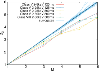
Figure 5: Variation of correlation dimension $D_{2}$ as a function of embedding dimension $M$ for classes V (ObsID 96420-01-06-03) and VIII (ObsID 96420-01-19-03). The different sets of energy bins in keV and the time bins in ms are indicated by various symbols. The lines without points are from surrogate data (see §5.2) and the straight diagonal black line represents the behaviour of an ideal stochastic system.

To mitigate against this possible effect, we further optimise both the energy band and the time bins. We carry out the analyses with increasing time bins from $0.125\,\mathrm{s}$ up to $1.0\,\mathrm{s}$ and energy bins of $2-8\,\mathrm{keV}$, $2-25\,\mathrm{keV}$, $2-60\,\mathrm{keV}$ and $8-25\,\mathrm{keV}$. The ratio $\langle PN\rangle/rms$ decreases by a few factors with increasing time bin, however the effect of reducing energy bin is only marginal. Figure 5 indicates that with increasing time bin, $D_{2}$ deviates from pure stochastic nature in classes V and VIII especially. This deviation is highlighted as nonstochasticity (NS) in Table 5. $\langle PN\rangle/rms$ values for time bin of $0.5\,\mathrm{s}$ in $2-60\,\mathrm{keV}$ are also shown in Table 5, which decrease with respect to those for $0.125\,\mathrm{s}$ reported in Table 4.

5.2 Surrogate data analysis

To place a greater level of confidence on any detected non-trivial structures in a time series, surrogate data analysis is normally applied. This has proven to be a very powerful method for differentiating signatures indicative of intrinsic fractal nature from coloured noise in time series, as shown in Fig. 5. The basic idea is to formulate a null hypothesis that the data has been generated by a stationary linear stochastic process and then by comparing results for the data with appropriate realisations of surrogate data, one attempts to reject this hypothesis. Surrogate data sets are normally generated such that they have the same distribution and power spectrum as the original data. One of the standard methods used for generating surrogates is the Iterative Amplitude Adjusted Fourier Transform (IAAFT) method (Schreiber & Schmitz, 1996, 2000), which is an improvement over the Amplitude Adjusted Fourier Transform (AAFT) technique (Theiler et al., 1992). We apply the scheme in this paper using the TISEAN package (Hegger et al., 1999). More detailed description of this method can be found in Misra et al. (2006) among others.

We use the normalised mean sigma deviation ($nmsd$), proposed by Harikrishnan et al. (2006), to quantify the differences in the discriminating measure between the data and the surrogates. This quantity is defined by

$$nmsd^{2}=\frac{1}{M_{max}-1}\mathop{\sum^{M_{max}}}_{M=M_{min}}{\left(\dfrac{D_{2}(M)-\langle D_{2}^{surr}(M)\rangle}{\sigma_{SD}^{surr}(M)}\right)},$$ (4)

where $M_{min}$ and $M_{max}$ are the minimum and maximum embedding dimensions respectively for which the analysis is carried out, $D_{2}^{surr}(M)$ is the $D_{2}$ value for surrogates at a given $M$, $\langle D_{2}^{surr}(M)\rangle$ is the average of $D_{2}^{surr}(M)$ and $\sigma_{SD}^{surr}(M)$ is the standard deviation of $D_{2}^{surr}(M)$. Harikrishnan et al. (2006) showed that a value of $nmsd<3.0$ indicates either white noise or coloured noise domination in the data and the null hypothesis cannot be rejected in such a case. On the other hand, when $nmsd>3$, the data may be considered distinguishable from its surrogates.

For better statistics, in our computation of $nmsd$, we use the lightcurves of bin size $0.5\,\mathrm{s}$ and generate $19$ surrogates for each of the ObsIDs representing the nine temporal classes of IGR J17091-3624. This is because, as shown by Schreiber & Schmitz (2000), $19$ surrogate time series are required for one-sided tests for a minimal significance requirement of $95\%$. In all cases, we fix $M_{min}=4$ in the estimation of $nmsd$ to exclude possible artefacts in the data at lower values of $M$. This is more justified since deterministic/fractal properties are designated based on $D_{2}$ at increasing $M$ and are preserved at higher values of $M$. The last column of Table 5 shows $nmsd$ values obtained for all $9$ temporal classes of IGR J17091-3624.

As discussed in §5.1, a few of the classes tend to show signatures of plausible higher dimensional chaos with higher time bins. Typical cases are classes V and VIII, shown in Fig. 5 as they can be seen to deviate from pure stochasticity at higher values of $M$. The behaviour of these two classes are referred to S/NS in Table 5. However, corresponding $nmsd$ values indicate that these deviations may not be significant. Longer, continuous observations with more modern X-ray telescopes providing more data points will be crucial to probe this better.

6 Discussions and conclusion

An accretion flow around a compact object is a nonlinear general relativistic system involving magnetohydrodynamics. Earlier, at least some of the accretion flows were argued to be similar to a Lorenz system (Misra et al., 2004; Mukhopadhyay, 2004; Misra et al., 2006; Karak et al., 2010), but contaminated by Poisson noise.

The large variability seen in GRS 1915+105 was interpreted by Belloni et al. (1997) to be the result of rapid removal and replenishment of matter in the hot accretion flow, which is driven by thermal-viscous instability in the disc. Since IGR J17091-3624 has been shown to mimic the variability properties seen in GRS 1915+105, it is natural to expect that the unique variability seen in both sources may be driven by the same physics (see, e.g., Capitanio et al., 2012).

Adegoke et al. (2018), in their study of the connection between observed spectra and nonlinear properties of GRS 1915+105, interpreted the accretion modes of the source in terms of four accretion classes, namely, Keplerian disc, slim disc, advection dominated accretion flow and general advective accretion flow. They also argued that accretion rate must play an important role in transition from one accretion mode to others. We therefore attempt to interpret our analysis results for IGR J17091-3624 in the line with this picture.

6.1 General features obtained in time series

For each of the $9$ temporal classifications of IGR J17091-3624, we probe their underlying nonlinear time series properties through correlation integral method – a method that has been established over the years as an efficient technique for understanding low-dimensional chaotic properties in time series. This can be typically quantified by the variation of correlation dimension $D_{2}$ against the embedding dimension $M$. In this way, the value of $D_{2}$ determines the effective number of differential equations describing the dynamics of the system and the variation of $D_{2}$ with $M$ reveals the nonlinear dynamical properties of the system. The system is considered deterministic if initially $D_{2}$ increases linearly with $M$ until it reaches a certain value and saturates. On the other hand, the system is stochastic if for all $M$, $D_{2}\approx M$ (see e.g., Misra et al., 2004; Mukhopadhyay, 2004; Adegoke et al., 2017).

Unlike in GRS 1915+105, where some of the temporal classes show signatures of low-dimensional fractal (or F) while others show signatures consistent with stochasticity (or S), for IGR J17091-3624 we find all $9$ classes to be stochastic in their time series behaviour as shown in Table 1. Equally all the lightcurves obtained with XMM-Newton and chandra show signatures consistent with stochasticity.

6.2 General features obtained in spectral analysis

We fit the energy spectra for all observations using XSPEC version $12.9.1$. Errors are quoted at the one sigma confidence level for all parameters. The two main components are the multi-colour disc blackbody model or diskbb (see, e.g., Mitsuda et al., 1984; Makishima et al., 1986) and a powerlaw model or PL. The multiplicative model tbabs is used to account for X-ray absorption by the inter-stellar medium (ISM), with the equivalent hydrogen column density $n_{H}$ fixed at $6.28\times 10^{21}\,\mathrm{{cm}^{-2}}$ (Kalberla et al., 2005). For Chandra and XMM-Newton data, $n_{H}$ was allowed to vary from $6.28\times 10^{21}\,\mathrm{{cm}^{-2}}$ to about a factor of 2 higher for acceptable fit parameters. The quantity ${\chi}^{2}/dof$ for classes I, IV and VIII gets improved considerably, from $70/45$, $59/45$ and $59/45$ to $48/43$, $45/43$ and $56/43$ respectively, with the inclusion of Gaussian line features fixed at $6.4\,\mathrm{keV}$ (representing Fe-$\textrm{K}_{\alpha}$ lines). The fit to the RXTE data of class IX gets worsened with the inclusion of Gaussian line at $6.4\,\mathrm{keV}$ with ${\chi}^{2}/dof$ changing from $71/45$ to $75/43$. All the other classes give acceptable spectral fits and do not require the inclusion of Gaussian line features. As evident in Table 1, four of the nine classes (VI, VII, VIII, IX) exhibit diskbb dominated spectrum (DD), four (I, II, III, IV) show PL dominated spectrum (PD), while one reveals almost equal contributions from diskbb and PL. We define a state to be PD if the ratio of contributions from PL to diskbb is $\gtrsim 4/3$, and DD if the ratio of contributions from diskbb to PL is $\gtrsim 4/3$. In terms of spectral properties, classes I, III, IV and IX are similar to those of their GRS 1915-like counterparts discussed in Adegoke et al. (2018). While class II represents a typical low-hard state with the lowest flux, class I may depict the hard intermediate state, being powerlaw dominated with a high flux (Belloni & Motta, 2016).

Of the four extreme combinations of accretion flows described by Adegoke et al. (2018) (namely: F & HS; S & HS; F & LH and S & LH), primarily two (S & HS and S & LH) can be defined for IGR J17091-3624. In the line with this classification, high-soft (HS) state showing S in a time series implies quasi-spherical but radiation trapped, optically thick flow revealing incoherent flux in time, otherwise known as slim disc and is usually associated with highest accretion rates (e.g. Abramowicz et al., 1988). On the other hand, low-hard (LH) state showing S in a time series is consistent with a flow that is optically thin, puffed-up and quasi-spherical, where random cooling processes result in incoherent flux making it stochastic and possessing strong radial advection and is typically associated with significantly low accretion rates, called general advective accretion flow (GAAF: Rajesh & Mukhopadhyay 2010). We posit that in IGR J17091-3624, depending on accretion rate, the flow switches from one accretion regime to another. At the high accretion rate (or the regime of highest accretion rate among four possible above mentioned cases, corresponding to “S & HS"), the flow mimics a slim disc which is radiation dominated and geometrically thicker than a Keplerian disc, which is seen in the temporal classes VI, VII, VIII and IX. At significantly low accretion rate (but not at the regime of lowest accretion rate, which corresponds to “F & LH", see Adegoke et al. 2018), the flow becomes hot, radiatively inefficient, optically thin and with significant advection, namely GAAF, as seen in the temporal classes I, II, III and IV. Indeed, Table 1 shows that on average the former four classes exhibit higher luminosity than latter ones, with the exception in class I, which has been explained above. This favours our apparently heuristic argument. However, the flow must pass through in between the Keplerian regime with intermediate accretion rates. This seems to be revealed in classes V and VIII at higher time bins with reduced Poisson noise, based on the analysis discussed in §5.1. Emergence of non-stochasticity in time series with DD spectral (HS) state indicates the flow to be between slim disc and Keplerian disc regimes (pure fractal nature would argue for a pure Keplerian flow). On the other hand, emergence of non-stochasticity along with D-P state favours the idea of the flow to be between Keplerian and GAAF regimes. Note that a DD state corresponds to higher accretion rate than a D-P state, which is indeed revealed from the respective flux reported in Table 1. Nevertheless, as discussed in §5.2, all the classes including V and VIII exhibit $nmsd<3$, arguing against any deterministic feature. Hence, longer time series data (which is not available for data sets under consideration at $1\,\mathrm{s}$ bin) are required to confirm this hypothesis. The future X-ray missions that can observe continuously for much longer duration may provide such required lightcurves and hence time series. Note that classes identified as slim discs should in principle be fitted with diskpbb rather than diskbb model in XSPEC. Hence, we have subsequently cross-verified that the underlying spectral fits indeed are consistent with diskpbb model and they are indeed consistent with slim discs.

Therefore, while the presence of plausibly significant level of Poisson noise in our data poses problem for comparison of the nonlinear timing properties of IGR J17091-3624 vis-a-vis GRS 1915+105, they seem to be following similar track, at least partially. This is because underlying low-dimensional fractal signature may have been suppressed, as the presence of noise can significantly affect $D_{2}-M$ relation and suppress any signatures of low dimensional chaos in a system (see, e.g., Misra et al., 2004, 2006). However, the stochastic nature may indeed be inherent in the lightcurves of IGR J17091-3624. If this is so, it implies that although IGR J17091-3624 and GRS 1915+105 show remarkable similarity in their exotic variability patterns, the underlying physics responsible for this may not be very same.

References

- Abramowicz et al. (1988) Abramowicz M. A., Czerny B., Lasota J. P., Szuszkiewicz E., 1988, ApJ, 332, 646
- Adegoke et al. (2017) Adegoke O., Rakshit S., Mukhopadhyay B., 2017, MNRAS, 466, 3951
- Adegoke et al. (2018) Adegoke O., Dhang P., Mukhopadhyay B., Ramadevi M. C., Bhattacharya D., 2018, MNRAS, 476, 1581
- Altamirano & Belloni (2012) Altamirano D., Belloni T., 2012, ApJ, 747, L4
- Altamirano et al. (2011) Altamirano D., et al., 2011, ApJ, 742, L17
- Ardito et al. (2017) Ardito A., Ricciardi P., Massaro E., Mineo T., Massa F., 2017, International Journal of Non Linear Mechanics, 88, 142
- Belloni & Motta (2016) Belloni T. M., Motta S. E., 2016, in Bambi C., ed., Astrophysics and Space Science Library Vol. 440, Astrophysics of Black Holes: From Fundamental Aspects to Latest Developments. p. 61 (arXiv:1603.07872), doi:10.1007/978-3-662-52859-4_2
- Belloni et al. (1997) Belloni T., Méndez M., King A. R., van der Klis M., van Paradijs J., 1997, ApJ, 479, L145
- Belloni et al. (2000) Belloni T., Klein-Wolt M., Méndez M., van der Klis M., van Paradijs J., 2000, A&A, 355, 271
- Capitanio et al. (2012) Capitanio F., Del Santo M., Bozzo E., Ferrigno C., De Cesare G., Paizis A., 2012, MNRAS, 422, 3130
- Castro-Tirado et al. (1992) Castro-Tirado A. J., Brandt S., Lund N., 1992, IAU Circ., 5590
- Court et al. (2017) Court J. M. C., Altamirano D., Pereyra M., Boon C. M., Yamaoka K., Belloni T., Wijnands R., Pahari M., 2017, MNRAS, 468, 4748
- Grassberger & Procaccia (1983) Grassberger P., Procaccia I., 1983, Phys. Rev. A, 28, 2591
- Grinberg et al. (2016) Grinberg V., et al., 2016, The Astronomer’s Telegram, 8761
- Harikrishnan et al. (2006) Harikrishnan K., Misra R., Ambika G., Kembhavi A., 2006, Physica D: Nonlinear Phenomena, 215, 137
- Hegger et al. (1999) Hegger R., Kantz H., Schreiber T., 1999, Chaos: An Interdisciplinary Journal of Nonlinear Science, 9, 413
- Jahoda et al. (1996) Jahoda K., Swank J. H., Giles A. B., Stark M. J., Strohmayer T., Zhang W., Morgan E. H., 1996, in Siegmund O. H., Gummin M. A., eds, Proc. SPIEVol. 2808, EUV, X-Ray, and Gamma-Ray Instrumentation for Astronomy VII. pp 59–70, doi:10.1117/12.256034
- Kalberla et al. (2005) Kalberla P. M. W., Burton W. B., Hartmann D., Arnal E. M., Bajaja E., Morras R., Pöppel W. G. L., 2005, A&A, 440, 775
- Karak et al. (2010) Karak B. B., Dutta J., Mukhopadhyay B., 2010, ApJ, 708, 862
- Krimm & Kennea (2011) Krimm H. A., Kennea J. A., 2011, The Astronomer’s Telegram, 3148
- Kuulkers et al. (2003) Kuulkers E., Lutovinov A., Parmar A., Capitanio F., Mowlavi N., Hermsen W., 2003, The Astronomer’s Telegram, 149
- Makishima et al. (1986) Makishima K., Maejima Y., Mitsuda K., Bradt H. V., Remillard R. A., Tuohy I. R., Hoshi R., Nakagawa M., 1986, ApJ, 308, 635
- Maselli et al. (2018) Maselli A., Capitanio F., Feroci M., Massa F., Massaro E., Mineo T., 2018, A&A, 612, A33
- Massaro et al. (2014) Massaro E., Ardito A., Ricciardi P., Massa F., Mineo T., D’Aì A., 2014, Ap&SS, 352, 699
- Miller et al. (2016) Miller J. M., Reynolds M., Kennea J., King A. L., Tomsick J., 2016, The Astronomer’s Telegram, 8742
- Misra et al. (2004) Misra R., Harikrishnan K. P., Mukhopadhyay B., Ambika G., Kembhavi A. K., 2004, ApJ, 609, 313
- Misra et al. (2006) Misra R., Harikrishnan K. P., Ambika G., Kembhavi A. K., 2006, ApJ, 643, 1114
- Mitsuda et al. (1984) Mitsuda K., et al., 1984, PASJ, 36, 741
- Mukhopadhyay (2004) Mukhopadhyay B., 2004, in Kaaret P., Lamb F. K., Swank J. H., eds, American Institute of Physics Conference Series Vol. 714, X-ray Timing 2003: Rossi and Beyond. pp 48–51 (arXiv:astro-ph/0402222), doi:10.1063/1.1780998
- Narayan & Yi (1994) Narayan R., Yi I., 1994, ApJ, 428, L13
- Pahari et al. (2014) Pahari M., Yadav J. S., Bhattacharyya S., 2014, ApJ, 783, 141
- Rajesh & Mukhopadhyay (2010) Rajesh S. R., Mukhopadhyay B., 2010, MNRAS, 402, 961
- Schreiber & Schmitz (1996) Schreiber T., Schmitz A., 1996, Phys. Rev. Lett., 77, 635
- Schreiber & Schmitz (2000) Schreiber T., Schmitz A., 2000, Physica D: Nonlinear Phenomena, 142, 346
- Shakura & Sunyaev (1973) Shakura N. I., Sunyaev R. A., 1973, A&A, 24, 337
- Theiler et al. (1992) Theiler J., Eubank S., Longtin A., Galdrikian B., Farmer J. D., 1992, Physica D: Nonlinear Phenomena, 58, 77