Exploring families of
energy-dissipation landscapes via tilting
— three types of EDP convergence

Abstract

We introduce two new concepts of convergence of gradient systems $({\mathbf{Q}},{\mathcal{E}}_{\varepsilon},{\mathcal{R}}_{\varepsilon})$ to a limiting gradient system $({\mathbf{Q}},{\mathcal{E}}_{0},{\mathcal{R}}_{0})$. These new concepts are called ‘EDP convergence with tilting’ and ‘contact–EDP convergence with tilting’. Both are based on the Energy-Dissipation-Principle (EDP) formulation of solutions of gradient systems, and can be seen as refinements of the Gamma-convergence for gradient flows first introduced by Sandier and Serfaty.

The two new concepts are constructed in order to avoid the ‘unnatural’ limiting gradient structures that sometimes arise as limits in EDP-convergence. EDP-convergence with tilting is a strengthening of EDP-convergence by requiring EDP-convergence for a full family of ‘tilted’ copies of $({\mathbf{Q}},{\mathcal{E}}_{\varepsilon},{\mathcal{R}}_{\varepsilon})$. It avoids unnatural limiting gradient structures, but many interesting systems are non-convergent according to this concept. Contact–EDP convergence with tilting is a relaxation of EDP convergence with tilting, and still avoids unnatural limits but applies to a broader class of sequences $({\mathbf{Q}},{\mathcal{E}}_{\varepsilon},{\mathcal{R}}_{\varepsilon})$.

In this paper we define these concepts, study their properties, and connect them with classical EDP convergence. We illustrate the different concepts on a number of test problems.

1 Introduction to gradient systems, gradient flows, and kinetic relations

1.1 Gradient systems

A gradient system is a triple $({\mathbf{Q}},{\mathcal{E}},{\mathcal{R}})$ of a state space ${\mathbf{Q}}$, a functional ${\mathcal{E}}$ on ${\mathbf{Q}}$, and a dissipation potential ${\mathcal{R}}$. This triple defines in a unique way a differential equation for the evolution $t\mapsto q(t)$ of the states, the so-called gradient-flow equation:

$$0={\mathrm{D}}_{\dot{q}}{\mathcal{R}}(q(t),\dot{q}(t))+{\mathrm{D}}{\mathcal{E}}(q(t)),$$ (1.1)

which can be seen as a balance of thermodynamical forces, namely the potential restoring force $-{\mathrm{D}}{\mathcal{E}}(q)$ and the viscous force $\xi={\mathrm{D}}_{\dot{q}}{\mathcal{R}}(q,\dot{q})$ induced by the rate $\dot{q}$. Indeed, any functional dependence $\xi=K(q,\dot{q})$ or $\dot{q}=G(q,\xi)$ between the rate $\dot{q}$ and the dual (viscous) friction force $\xi$ is often called a kinetic relation. Gradient-flow equations are distinguished by two facts:

• the kinetic relation $K$ is given as a (sub)differential of a dissipation potential,
  i.e. $K(q,\dot{q})={\mathrm{D}}_{\dot{q}}{\mathcal{R}}(q,\dot{q})$, and

• the viscous force $\xi$ is counterbalanced by a potential restoring force, i.e. $\xi=-{\mathrm{D}}{\mathcal{E}}(q)$.

These two conditions allow for a variational characterization for the gradient-flow equation (1.1), the so-called energy-dissipation principle, which is the basis of this work; see Section 2 for this and a more detailed description to gradient systems.

Using the Fenchel-Legendre transform one can define a dual dissipation potential ${\mathcal{R}}^{*}(q,\xi)$ such that the kinetic relation can be written through any of the three equivalent conditions

$$\xi=K(q,v)={\mathrm{D}}_{v}{\mathcal{R}}(q,v),$$ (1.2)

$$v=G(q,\xi)={\mathrm{D}}_{\xi}{\mathcal{R}}^{*}(q,\xi),\qquad\text{or}$$

$${\mathcal{R}}(q,v)+{\mathcal{R}}^{*}(q,\xi)=\langle\xi,v\rangle.$$

While, for a given gradient system $({\mathbf{Q}},{\mathcal{E}},{\mathcal{R}})$, the gradient-flow equation (1.1) is uniquely given and may be rewritten in the form

$$\dot{q}={\mathbf{V}}(q)\coloneqq{\mathrm{D}}_{\xi}{\mathcal{R}}^{*}(q,{-}{\mathrm{D}}{\mathcal{E}}(q))=G(q,{-}{\mathrm{D}}{\mathcal{E}}(q)),$$ (1.3)

the opposite direction, however, shows a strong non-uniqueness for a given vector field ${\mathbf{V}}$ and a given energy ${\mathcal{E}}$ there may be many kinetic relations $G$, and even many dual dissipation potentials ${\mathcal{R}}^{*}$, such that ${\mathbf{V}}$ is generated as in (1.3).

We say that that the differential equation $\dot{q}={\mathbf{V}}(q)$ has the gradient structure $({\mathbf{Q}},{\mathcal{E}},{\mathcal{R}})$ if ${\mathbf{V}}(q)={\mathrm{D}}_{\xi}{\mathcal{R}}^{*}(q,{-}{\mathrm{D}}{\mathcal{E}}(q))$. Adding such a gradient structure to a differential equation means to identify additional thermodynamical information that is no longer visible in the induced gradient-flow equation $\dot{q}={\mathbf{V}}(q)$.

1.2 First example: a simple spring-damper system

$q$ [t] at 54 1 $k$ [b] at 36 23 $\mu$ [b] at 76 27

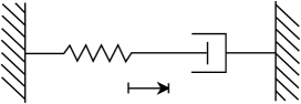
Figure 1.1: A spring-damper system. The spring has spring constant $k$, and the damper has the viscosity constant $\mu$.

We first illustrate the concept of a gradient system with an example, in which a spring relaxes by moving a damper (a shock absorber), see Figure 1.1. The state of the system is the spring displacement $q\in{\mathbb{R}}$, the energy contained in the spring is ${\mathcal{E}}_{1}(q)\coloneqq kq^{2}/2$, and the spring exerts a force $\xi$ equal to the negative derivative $-{\mathrm{D}}{\mathcal{E}}_{1}(q)=-kq$ of the energy. The damper is defined by the property that its rate $v$ of displacement is related to the force $\xi$ on the damper by $\mu v=\xi$, for some coefficient $\mu>0$. By combining these two relations we find the evolution equation for the state $q$,

$$\mu\dot{q}=-kq.$$ (1.4)

We identify equation (1.4) as the gradient-flow equation for $({\mathbb{R}},{\mathcal{E}}_{1},{\mathcal{R}}_{1})$, when we observe that the damper relation $\mu v=\xi$ can also be written in terms of a dissipation potential ${\mathcal{R}}_{1}(v)\coloneqq\mu v^{2}/2$ and its Legendre dual ${\mathcal{R}}_{1}^{*}(\xi)\coloneqq\xi^{2}/(2\mu)$. The dissipation potential ${\mathcal{R}}_{1}$ defines the kinetic relation $\mu v=\xi$.

In this example, one readily recognizes a ‘classical’ spring energy in ${\mathcal{E}}_{1}(q)=kq^{2}/2$, and the quadratic form of ${\mathcal{R}}_{1}(v)=\mu v^{2}/2$ is a natural choice for a damper (see e.g. [Pel14, Ch. 5]). However, other gradient-flow formulations for the same evolution equation (1.4) exist, if ${\mathcal{R}}={\mathcal{R}}(q,v)$ may depend not only on the rate $v=\dot{q}$ but also on the state $q$:

$${\mathcal{E}}_{2} \coloneqq{\mathcal{E}}_{1}, \qquad{\mathcal{E}}_{3} \coloneqq{\mathcal{E}}_{1},$$

$${\mathcal{R}}_{2}(q,v) \coloneqq\frac{\mu}{1{+}\alpha k^{2}q^{2}/\mu^{2}}\Bigl{(}\frac{1}{2}v^{2}+\frac{\alpha}{4}v^{4}\Bigr{)}, \qquad{\mathcal{R}}_{3}(q,v) \coloneqq\frac{kq}{1{-}{\mathrm{e}}^{-kq/\mu}}\bigl{(}{\mathrm{e}}^{v}{-}v{-}1\bigr{)}.$$

All the systems $({\mathbb{R}},{\mathcal{E}}_{i},{\mathcal{R}}_{i})$ generates the same equation (1.4) via ${\mathrm{D}}_{v}{\mathcal{R}}_{i}(q,\dot{q})=-{\mathrm{D}}{\mathcal{E}}_{i}(q)$.

In fact, even in this simple scalar example, one can generate a wide variety of gradient systems for the same equation (1.4): take any smooth and convex $\psi\colon{\mathbb{R}}\to{\mathbb{R}}$ with $\min\psi=\psi(0)=0$, define $\varphi(q)=-kq/\psi^{\prime}(-kq/\mu)$ and ${\mathcal{R}}_{\psi}(q,v)\coloneqq\varphi(q)\psi(v)$, and then the gradient system $({\mathbb{R}},{\mathcal{E}}_{1},{\mathcal{R}}_{\psi})$ will generate equation (1.4). The two examples ${\mathcal{R}}_{2}$ and ${\mathcal{R}}_{3}$ above are both of this type.

These dissipation potentials might well be considered less ‘natural’ than ${\mathcal{R}}_{1}$. To start with, it is not obvious which modeling arguments would lead to the kinetic relations of ${\mathcal{R}}_{2}$ and ${\mathcal{R}}_{3}$, which are

$$\mu\bigl{(}v{+}\alpha v^{3}\bigr{)}=\Bigl{(}1{+}\alpha\frac{k^{2}q^{2}}{\mu^{2}}\Bigr{)}\,\xi\quad\text{(for ${\mathcal{R}}_{2}$)},\qquad\text{and}\quad{\mathrm{e}}^{v}-1=\frac{1-{\mathrm{e}}^{-kq/\mu}}{kq}\,\xi\quad\text{(for ${\mathcal{R}}_{3}$).}$$

In addition, a definition like that of ${\mathcal{R}}_{3}$ is dimensionally inconsistent, since arguments of the exponential function should be dimensionless. Both these problems are related to a deeper and more troubling problem: the dissipation potentials depend not only on $\mu$ but also on $k$, implying that the kinetic relation generated by ${\mathcal{R}}_{2}$ or ${\mathcal{R}}_{3}$, which is supposed to characterize the damper, depends on the strength $k$ of the spring. This is an unsatisfactory situation: we consider the spring and the damper to be two independent objects, and their mathematical characterizations should therefore also be independent.

This example points towards the problem that we aim to solve in this paper. This problem arises especially when taking limits of gradient systems in some parameter $\varepsilon\to 0$; in such limits it is unavoidable that the limiting dissipation potential depends on the state $q$ as well as the rate of change $v$. As a result, the limiting evolution equation will have many gradient-flow structures, as in the example above. It turns out that one of the most common concepts used to define limits of gradient systems, which we call ‘simple EDP convergence’ in this paper and which we explain below, often selects limit dissipation potentials that are ‘unhealthy’ in the same way as ${\mathcal{R}}_{2}$ and ${\mathcal{R}}_{3}$ are ‘unhealthy’: they depend on aspects of the energy in an unsatisfactory way.

The aim of this paper is to construct alternative convergence concepts that lead to limiting gradient systems that are more ‘natural’ or ‘healthy’. What we mean by these terms will become clear below, but first we consider an example to further illustrate the problem.

1.3 Second example: wiggly dissipation

In Section 3 we study the following example in detail. Consider a family of gradient systems $({\mathbb{R}},{\mathcal{E}},{\mathcal{R}}_{\varepsilon})$, indexed by $\varepsilon>0$, where ${\mathcal{E}}$ is some smooth $\varepsilon$-independent function, and

$${\mathcal{R}}_{\varepsilon}(q,v)\coloneqq\frac{1}{2}\mu\Bigl{(}q,\frac{q}{\varepsilon}\Bigr{)}\,v^{2}.$$

Here $\mu\in{\mathrm{C}}^{0}({\mathbb{R}}^{2})$ is positive and $1$-periodic in the second variable. For this ‘wiggly dissipation’ system the gradient-flow equation takes the form

$$\mu\Bigl{(}q,\frac{q}{\varepsilon}\Bigr{)}\,\dot{q}=-{\mathrm{D}}{\mathcal{E}}(q).$$ (1.5)

An example of a solution is given in Figure 1.2.

Figure 1.2: A simulation of the solution $q_{\varepsilon}$ (blue) and the limit solution $q_{0}(t)={\mathrm{e}}^{-t}$ (violet) for the system $(1{+}0.8\cos(2\pi\,q/\varepsilon))\,\dot{q}=-q$ with $q(0)=1$ and $\varepsilon=0.2$. The solution has regions of slow and of fast decay depending on the size of $1{+}0.8\cos(2\pi\,q/\varepsilon)\in[0.2,1.8]$.

We show in Section 3 that for $\varepsilon\to 0$, the solutions $q_{\varepsilon}$ of (1.5) converge to limit functions $q_{0}$ that solve the limiting equation

$$\macc@depth\char 1\relax\frozen@everymath{\macc@group}\macc@set@skewchar\macc@nested@a 111{}(q)\,\dot{q}=-{\mathrm{D}}{\mathcal{E}}(q)\qquad\text{with}\quad\macc@depth\char 1\relax\frozen@everymath{\macc@group}\macc@set@skewchar\macc@nested@a 111{}(q)=\int_{0}^{1}\mu(q,y)\;\!\mathrm{d}y.$$ (1.6)

In fact, $({\mathbb{R}},{\mathcal{E}},{\mathcal{R}}_{\varepsilon})$ converges in the simple EDP sense (defined in Section 2.3) to a limiting system $({\mathbb{R}},{\mathcal{E}},\widetilde{\mathcal{R}}_{0})$, where

$$\widetilde{\mathcal{R}}_{0}(q,v)\coloneqq{\mathcal{M}}_{0}(q,v,-{\mathrm{D}}{\mathcal{E}}(q))-{\mathcal{M}}_{0}(q,0,-{\mathrm{D}}{\mathcal{E}}(q)),$$ (1.7a)

and $${\mathcal{M}}_{0}$$ is defined via

$${\mathcal{M}}_{0}(q,v,\xi)=\inf\Big{\{}\int_{s=0}^{1}\!\!\Big{(}\frac{\mu(q,z(s))\big{(}vz^{\prime}(s)\big{)}^{2}}{2}+\frac{\xi^{2}}{2\mu(q,z(s))}\Big{)}\;\!\mathrm{d}s\;\Big{|}$$ (1.7b)

$$z\colon[0,1]\to{\mathbb{R}},\ z(1)=z(0)+\mathop{\mathrm{sign}}(v) \Big{\}},$$

We verify explicitly in Section 3 that the system $({\mathbb{R}},{\mathcal{E}},\widetilde{\mathcal{R}}_{0})$ indeed generates equation (1.6), i.e. that

$$\macc@depth\char 1\relax\frozen@everymath{\macc@group}\macc@set@skewchar\macc@nested@a 111{}(q)\,\dot{q}=-{\mathrm{D}}{\mathcal{E}}(q)\qquad\Longleftrightarrow\qquad{\mathrm{D}}_{v}\widetilde{\mathcal{R}}_{0}(q,\dot{q})=-{\mathrm{D}}{\mathcal{E}}(q).$$

However, this limiting dissipation potential $\widetilde{\mathcal{R}}_{0}$ suffers from the same problem as ${\mathcal{R}}_{2}$ and ${\mathcal{R}}_{3}$ above: it depends explicitly on the energy function ${\mathcal{E}}$, as is clear from (1.7a). If one repeats the simple EDP convergence theorem for a perturbed energy ${\mathcal{E}}+{\mathcal{F}}$ with an arbitrary tilting function ${\mathcal{F}}$, then ${\mathcal{F}}$ propagates into the formula (1.7a) for $\widetilde{\mathcal{R}}_{0}$; changing the energy thus leads to a different dissipation potential $\widetilde{\mathcal{R}}_{0}$. As above, we consider this unsatisfactory, since the energy driving the system is conceptually separate from the mechanism for dissipating that energy.

In contrast, if we disregard the fact that equation (1.6) arises as a limit, and consider it as an isolated system, then we might conjecture a gradient structure with the effective dissipation potential ${\mathcal{R}}_{\mathrm{eff}}(q,v)\coloneqq\macc@depth\char 1\relax\frozen@everymath{\macc@group}\macc@set@skewchar\macc@nested@a 111{}(q)\,v^{2}/2$ instead. Indeed, combined with the energy ${\mathcal{E}}$ this potential ${\mathcal{R}}_{\mathrm{eff}}$ also generates equation (1.6); it is much simpler to interpret than $\widetilde{\mathcal{R}}_{0}$, and most importantly, it does not depend on ${\mathcal{E}}$.

1.4 Towards a better convergence concept

These examples show that we have on one hand an unsatisfactory convergence result, in which $({\mathbb{R}},{\mathcal{E}},\widetilde{\mathcal{R}}_{0})$ is proven to arise as the unique limit of the family $({\mathbb{R}},{\mathcal{E}},{\mathcal{R}}_{\varepsilon})$ in the simple EDP sense, but this limit is unsatisfactory as a description of a gradient system.

On the other hand, the alternative dissipation potential ${\mathcal{R}}_{\mathrm{eff}}$ generates the same limit equation and does not suffer from the philosophical problems associated with $\widetilde{\mathcal{R}}_{0}$. Its only drawback is that the system $({\mathbb{R}},{\mathcal{E}},{\mathcal{R}}_{\mathrm{eff}})$ is not the limit of the family $({\mathbb{R}},{\mathcal{E}},{\mathcal{R}}_{\varepsilon})$ in the simple EDP sense.

As mentioned above, these observations strongly suggest seeking alternative convergence concepts for gradient systems, which should generate limiting potentials that do not depend on the limiting energy. Specifically, we will seek convergence concepts—let us indicate them with ‘$\square$’—that have the following property: if

$$({\mathbf{Q}},{\mathcal{E}}_{\varepsilon},{\mathcal{R}}_{\varepsilon})\overset{\square}{\longrightarrow}({\mathbf{Q}},{\mathcal{E}}_{0},{\mathcal{R}}_{0}),$$ (1.8)

then for all ${\mathcal{F}}\in{\mathrm{C}}^{1}({\mathbf{Q}})$ we also have

$$({\mathbf{Q}},\,{\mathcal{E}}_{\varepsilon}{+}{\mathcal{F}},\,{\mathcal{R}}_{\varepsilon})\overset{\square}{\longrightarrow}({\mathbf{Q}},\,{\mathcal{E}}_{0}{+}{\mathcal{F}},\,{\mathcal{R}}_{0}),$$ (1.9)

where the dissipation potential ${\mathcal{R}}_{0}$ in (1.9) is the same as in (1.8), and therefore does not depend on the tilt function ${\mathcal{F}}$.

Indeed, the two new concepts that we introduce in Section 2.6 both have this property, and we show in Section 3 that, by applying one of these convergence concepts, we indeed find the more natural dissipation potential ${\mathcal{R}}_{\mathrm{eff}}$ rather than $\widetilde{\mathcal{R}}_{0}$.

1.5 The larger picture: effective kinetic relations

Our aim of deriving ‘healthy’ limiting gradient systems could also be formulated as the challenge of deriving effective kinetic relations. We already introduced a kinetic relation as a relation between a force $\xi$ and a rate $v=\dot{q}$. An important class of such kinetic relations arises naturally in gradient systems, since dissipation potentials ${\mathcal{R}}$ define kinetic relations via the three equivalent relations (1.2).

In view of the Young-Fenchel inequality ${\mathcal{R}}(q,v)+{\mathcal{R}}^{*}(q,\xi)\geq\langle\xi,v\rangle\color[rgb]{0,0,0}$, which holds generally for Legendre conjugate pairs $({\mathcal{R}},{\mathcal{R}}^{*})$, and the third formulation in (1.2), we define the contact set as the set of pairs $(v,\xi)$:

$${\mathcal{C}}={\mathcal{C}}_{{\mathcal{R}}\oplus{\mathcal{R}}^{*}}(q) \coloneqq\Big{\{}\>\!(v,\xi)\in{\mathbf{Q}}\times{\mathbf{Q}}^{*}\;\Big{|}\;{\mathcal{R}}(q,v)+{\mathcal{R}}^{*}(q,\xi)=\langle\xi,v\rangle\color[rgb]{0,0,0}\>\!\Big{\}}$$

$$=\mathop{\mathrm{graph}}\bigl{(}{\mathrm{D}}_{v}{\mathcal{R}}(q,\cdot)\bigr{)}.$$

This set ${\mathcal{C}}$ characterizes the pairs of rates $v$ and forces $\xi$ that are admissible to the system, and thus determine the kinetic relation. As was already mentioned, the equation generated by the gradient system can be viewed as the result of applying the kinetic relation $(v,\xi)\in{\mathcal{C}}_{{\mathcal{R}}\oplus{\mathcal{R}}^{*}}(q)$ to a context where the force $\xi$ is generated by the potential ${\mathcal{E}}$:

$$\xi=-{\mathrm{D}}{\mathcal{E}}(q)\qquad\text{and}\qquad(\dot{q},\xi)\in{\mathcal{C}}_{{\mathcal{R}}\oplus{\mathcal{R}}^{*}}(q).$$ (1.10)

Kinetic relations appear throughout physics and mechanics. Well-known examples are Stokes’ law $\xi=6\pi\eta R\,v$ for the drag force $\xi$ on a sphere dragged through a viscous fluid (where $\eta$ is the dynamic viscosity and $R$ the radius of the sphere), power-law viscous relationships of the form $\xi=c\lvert v\rvert^{p-1}v$, and Coulomb friction $\xi\in c\operatorname{Sign}(v)$, where $\operatorname{Sign}$ is the subdifferential of the absolute value. These examples show that the relationship may be linear or nonlinear, and single- or multi-valued. A priori, there is no reason why a kinetic relation should be the graph of the derivative of a dissipation potential, but here we are interested in the ones that do have that property. The reasoning for the restriction of kinetic relations in form of subdifferentials, i.e. $\xi={\mathrm{D}}_{v}{\mathcal{R}}(q,v)$, is twofold. First, they define gradient systems and thus lead to variational characterizations for the gradient flow (see Section 2.2). Secondly, dissipation potentials arise naturally from thermodynamic principles derived from microscopic stochastic models via large-deviation principles; see Section 6 and [AD^∗11, MPR14, PRV14, MP^∗17]. Moreover, Onsager’s fundamental symmetry relation ${\mathbb{G}}={\mathbb{G}}^{*}$ for the linear kinetic relation $\xi={\mathbb{G}}v$ (see [Ons31]) is equivalent to the existence of a (quadratic) dissipation potential ${\mathcal{R}}(v)=\frac{1}{2}\langle{\mathbb{G}}v,v\rangle$.

We now turn to the challenge of deriving effective kinetic relations. We are given a family of kinetic relations parametrized by $\varepsilon$. The interpretation of $\varepsilon$ as a small parameter, or a small scale, often implies that there are natural ‘macroscopic,’ ‘averaged,’ or ‘effective’ forces and rates, which reflect the behavior of the true forces and rates in the system at scales that are large with respect to $\varepsilon$, while smoothing out the behavior at smaller scales. To derive an effective kinetic relation means to find a new relation between the limits of such macroscopic forces and rates as $\varepsilon\to 0$, leading to a characterization of the kinetic relation for ‘the limiting system’.

Again, these effective kinetic relations are very common; for instance, Stokes’ law, Fourier’s law, Fick’s law, and many similar laws actually are effective kinetic relations, derived from more microscopic systems, often consisting of particles. Throughout science, such effective kinetic relations are the starting point for the modeling of dissipative systems at an effective scale [Ött05, Ber07, Mie11, Pel14]. A detailed understanding of the properties and assumptions that lie at the basis of such effective kinetic relations is therefore essential.

We now return to the question of what we mean by a ‘healthy’ and an ‘unhealthy’ kinetic relation. The limiting dissipation potential $\widetilde{\mathcal{R}}_{0}$ in the second example above depends on the energy ${\mathcal{E}}$, i.e. $\widetilde{\mathcal{R}}_{0}(q,v)=\macc@depth\char 1\relax\frozen@everymath{\macc@group}\macc@set@skewchar\macc@nested@a 111{}_{-{\mathrm{D}}{\mathcal{E}}(q)}(q,v)$. It follows that the contact set ${\mathcal{C}}_{\macc@depth\char 1\relax\frozen@everymath{\macc@group}\macc@set@skewchar\macc@nested@a 111{}_{-{\mathrm{D}}{\mathcal{E}}}\oplus\macc@depth\char 1\relax\frozen@everymath{\macc@group}\macc@set@skewchar\macc@nested@a 111{}_{-{\mathrm{D}}{\mathcal{E}}}^{*}}$ also depends on ${\mathrm{D}}{\mathcal{E}}$. The gradient-flow equation (1.10) then takes the self-referential form

$$(\dot{q},-{\mathrm{D}}{\mathcal{E}}(q))\in{\mathcal{C}}_{\macc@depth\char 1\relax\frozen@everymath{\macc@group}\macc@set@skewchar\macc@nested@a 111{}_{-{\mathrm{D}}{\mathcal{E}}}\oplus\macc@depth\char 1\relax\frozen@everymath{\macc@group}\macc@set@skewchar\macc@nested@a 111{}_{-{\mathrm{D}}{\mathcal{E}}}^{*}}.$$

The induced evolution equation is correct, since the different occurrences of ${\mathrm{D}}{\mathcal{E}}(q)$ interact nicely. However, the set ${\mathcal{C}}_{{\mathcal{R}}_{-{\mathrm{D}}{\mathcal{E}}}\oplus{\mathcal{R}}_{-{\mathrm{D}}{\mathcal{E}}}^{*}}$ does not make sense as an independent kinetic relation, because ${\mathcal{C}}_{{\mathcal{R}}_{-{\mathrm{D}}{\mathcal{E}}}\oplus{\mathcal{R}}_{-{\mathrm{D}}{\mathcal{E}}}^{*}}$ does not provide us with valid information about admissible pairs $(v,\xi)$ other than for the case $\xi=-{\mathrm{D}}{\mathcal{E}}(q)$. In order to find the rate $\dot{q}$ for a force $\widehat{\xi}\neq-{\mathrm{D}}{\mathcal{E}}(q)$, we would need to construct a different energy $\widehat{\mathcal{E}}(q)$ such that $\widehat{\xi}=-{\mathrm{D}}\widehat{\mathcal{E}}(q)$, repeat the convergence process for this energy $\widehat{\mathcal{E}}$, obtain a different limiting dissipation potential $\widehat{\mathcal{R}}_{-{\mathrm{D}}\widehat{\mathcal{E}}}$, and read off the admissible rate $\dot{q}$ from the resulting contact set ${\mathcal{C}}_{\widehat{\mathcal{R}}_{-{\mathrm{D}}\widehat{\mathcal{E}}}\oplus\widehat{\mathcal{R}}_{-{\mathrm{D}}\widehat{\mathcal{E}}}^{*}}$. Since this latter set is generically different from ${\mathcal{C}}_{\macc@depth\char 1\relax\frozen@everymath{\macc@group}\macc@set@skewchar\macc@nested@a 111{}_{-{\mathrm{D}}{\mathcal{E}}}\oplus\macc@depth\char 1\relax\frozen@everymath{\macc@group}\macc@set@skewchar\macc@nested@a 111{}_{-{\mathrm{D}}{\mathcal{E}}}^{*}}$, this shows how a single contact set ${\mathcal{C}}_{\macc@depth\char 1\relax\frozen@everymath{\macc@group}\macc@set@skewchar\macc@nested@a 111{}_{-{\mathrm{D}}{\mathcal{E}}}\oplus\macc@depth\char 1\relax\frozen@everymath{\macc@group}\macc@set@skewchar\macc@nested@a 111{}_{-{\mathrm{D}}{\mathcal{E}}}^{*}}$ cannot be considered as a kinetic relation.

Instead, we seek a limiting kinetic relation that is defined as one single set ${\mathcal{C}}$ of pairs $(v,\xi)$ that provides us with all admissible combinations. The convergence concepts that we construct below are constructed with this aim in mind.

1.6 Third example: wiggly energy

In the example of Section 1.3 the ‘correct’ effective dissipation potential ${\mathcal{R}}_{\mathrm{eff}}(q,v)=\macc@depth\char 1\relax\frozen@everymath{\macc@group}\macc@set@skewchar\macc@nested@a 111{}(q)v^{2}/2$ is obtained solely from information encoded in ${\mathcal{R}}_{\varepsilon}$. When considering a family of $\Gamma$-converging energies ${\mathcal{E}}_{\varepsilon}\xrightarrow{\Gamma}{\mathcal{E}}_{0}$, however, the ‘correct’ limiting dissipation potential may also contain information from ${\mathcal{E}}_{\varepsilon}$. This may seem to contradict our claim from above that the dependence of the effective dissipation on the energy is ‘unhealthy’. As we shall see below, however, ‘correct’ or ‘healthy’ will mean that the effective dissipation potential ${\mathcal{R}}_{\mathrm{eff}}$ can depend on ‘microscopic details’ of ${\mathcal{E}}_{\varepsilon}$ but not on its ‘macroscopic limit’ ${\mathcal{E}}_{0}$. This expectation is stimulated by the idea of deriving a proper decomposition of ‘energy storage’ and ‘dissipation mechanisms’ in the macroscopic level.

To illustrate this we revisit the classical example of a gradient flow in a ‘wiggly’ energy landscape [Pra28, Jam96, ACJ96, DFM19]. Again we take as state space ${\mathbf{Q}}={\mathbb{R}}$, but now the energy ${\mathcal{E}}_{\varepsilon}$ is $\varepsilon$-dependent while the dissipation potential ${\mathcal{R}}_{\varepsilon}={\mathcal{R}}$ does not depend on $\varepsilon$:

$${\mathcal{E}}_{\varepsilon}(q)\coloneqq{\mathcal{E}}_{0}(q)+\varepsilon A(q)\cos\big{(}\tfrac{1}{\varepsilon}q\big{)},\qquad{\mathcal{R}}(v)\coloneqq\frac{\varrho(q)}{2}\,v^{2},$$ (1.11)

where ${\mathcal{E}}_{0}\colon{\mathbb{R}}\to{\mathbb{R}}$ is smooth and $\varrho\colon{\mathbb{R}}\to{\mathbb{R}}$ and $A\colon{\mathbb{R}}\to{\mathbb{R}}$ are smooth and positive. The induced gradient-flow evolution equation is

$$\varrho(q)\color[rgb]{0,0,0}\,\dot{q}=-{\mathrm{D}}{\mathcal{E}}_{0}(q)-\varepsilon A^{\prime}(q)\cos\big{(}\tfrac{1}{\varepsilon}q\big{)}+A(q)\sin\big{(}\tfrac{1}{\varepsilon}q\big{)}.$$

In Section 4 we summarize the results of [DFM19] and place them in the context of this paper. We find that the system $({\mathbb{R}},{\mathcal{E}}_{\varepsilon},{\mathcal{R}})$ converges in the simple EDP sense to a limiting system $({\mathbb{R}},{\mathcal{E}}_{0},\widetilde{\mathcal{R}}_{0})$, where ${\mathcal{E}}_{0}$ is the $\varepsilon$-independent part of ${\mathcal{E}}_{\varepsilon}$ as in (1.11), and $\widetilde{\mathcal{R}}_{0}$ is given by

$$\widetilde{\mathcal{R}}_{0}(q,v)={\mathcal{M}}_{0}(q,v,-{\mathrm{D}}{\mathcal{E}}_{0}(q))-{\mathcal{M}}_{0}(q,0,-{\mathrm{D}}{\mathcal{E}}_{0}(q)),$$

where this time the function ${\mathcal{M}}_{0}$ is given by

$${\mathcal{M}}_{0}(q,v,\xi)=\inf\Big{\{}\>\int_{0}^{1}\Bigl{[}\frac{\varrho(q)}{2}\,v^{2}\dot{z}^{2}(s) +\frac{\bigl{(}\xi{+}A\sin(z(s))\bigr{)}^{2}}{2\varrho(q)}\Bigr{]}\;\!\mathrm{d}s\>\;\Big{|}$$ (1.12)

$$z\colon[0,1]\to{\mathbb{R}},\ z(1)=z(0)+\mathop{\mathrm{sign}}(v)\;\Big{\}}.$$

As in the previous example, $\widetilde{\mathcal{R}}_{0}$ again depends on ${\mathrm{D}}{\mathcal{E}}_{0}(q)$. In Section 4 we also show that in the sense of one of the two new convergence concepts, namely contact EDP convergence with tilting, the family $({\mathbb{R}},{\mathcal{E}}_{\varepsilon},{\mathcal{R}})$ converges to a limiting system $({\mathbb{R}},{\mathcal{E}}_{0},{\mathcal{R}}_{\mathrm{eff}})$. Now, the effective dissipation potential ${\mathcal{R}}_{\mathrm{eff}}$ can be characterized explicitly via

$${\mathcal{R}}_{\mathrm{eff}}(q,v)=\int_{0}^{\lvert v\rvert}\sqrt{A(q)^{2}{+}(\varrho(q)w)^{2}}\,\;\!\mathrm{d}w.$$

We see that ${\mathcal{R}}_{\mathrm{eff}}$ is independent of ${\mathcal{E}}_{0}$ but it depends on $A$, which is microscopic information contained in the family ${\mathcal{E}}_{\varepsilon}$. Moreover, the quadratic structure of $v\mapsto{\mathcal{R}}(q,v)=\varrho(q)v^{2}/2$ is lost, because ${\mathcal{R}}_{\mathrm{eff}}(q,v)=\lvert A(q)v\rvert+O(\lvert v\rvert^{3})$ for $v\to 0$.

1.7 Tilt-EDP and contact-EDP convergence

The reason why gradient-flow convergence does not necessarily lead to a ‘healthy’ kinetic relation is relaxation: for a given macroscopic rate $v$ and force $\xi$, the limiting dissipation potential is found by a minimization over microscopic degrees of freedom constrained to the macroscopic imposed rate. This can be recognized in the definitions of ${\mathcal{M}}_{0}$ in (1.7b) and (1.12), and is very similar to the cell problems that arise in homogenization [Hor97, CiD99, Bra02]. In the cases of this paper, the solutions of these cell problems may not be of gradient-flow type, leading to a situation where the limit problem does not describe a gradient-flow structure. We analyze this in more detail in Section 5.

To correct this, we introduce two novel aspects. The first is to consider not a single family $({\mathbf{Q}},{\mathcal{E}}_{\varepsilon},{\mathcal{R}}_{\varepsilon})$ of gradient systems, but a full class of perturbed versions of this family. We perturb the given energies ${\mathcal{E}}_{\varepsilon}$ by arbitrary functions ${\mathcal{F}}\in{\mathrm{C}}^{1}({\mathbf{Q}})$:

$${\mathcal{E}}_{\varepsilon}^{\mathcal{F}}\coloneqq{\mathcal{E}}_{\varepsilon}+{\mathcal{F}}.$$

We call such a perturbation a ‘tilt’, and will then require convergence of all tilted systems simultaneously. The freedom to choose arbitrary tilts ${\mathcal{F}}$ allows us to probe the whole space of rates $v$ and forces $\xi$ for each $q$.

This setup leads to a first new convergence concept, which we call EDP convergence with tilting, or shortly tilt-EDP convergence. Unfortunately, it may suffer from the same problems of relaxation, and therefore it is a rather restrictive concept that is too strong to cover the simple cases of wiggly dissipation and wiggly energy discussed above.

The second new aspect is to weaken the definition of tilt-EDP convergence to require only a reduced connection between the relaxed problem and the limiting dissipation potential—a connection that only holds ‘at the contact set ${\mathcal{C}}$’. This leads to the concept of contact-EDP convergence with tilting, or shortly contact-EDP convergence. We show in the examples later in this paper that the concept of contact-EDP convergence for gradient systems yields kinetic relations that do not suffer from the force dependence that we observed above for simple EDP convergence.

1.8 Setup of the paper

In Section 2 we define gradient systems and gradient flows, recall the existing concept of simple EDP convergence, and introduce the two novel convergence concepts tilt-EDP convergence and contact-EDP convergence. These notions were already introduced in [DFM19], but called ‘strict EDP convergence’ and ‘relaxed EDP convergence’, respectively. In Section 3 and 4 we study in detail the examples of a wiggly dissipation potential and a wiggly energy, respectively, that were briefly mentioned above. In Section 5 we discuss in depth the reasons why the concept of contact-EDP convergence is an improvement over the classical concept of EDP convergence, and why it corrects the ‘incorrect’ kinetic relationship that we mentioned above.

In Section 6 we connect the tilting of energies as described above with tilting of random variables in large-deviation principles, and show how the independence of the dissipation potential from the force arises naturally in that context.

In Section 7 we present a result on tilt-EDP convergence that was formally derived in [LM^∗17] and is rigorously treated in [FrM19]. It concerns diffusion through a membrane in the limit of vanishing thickness and shows that even in the case of tilt-EDP convergence we can start with quadratic dissipation potentials ${\mathcal{R}}_{\varepsilon}(q,\cdot)$, i.e. linear kinetic relations, and end up with a non-quadratic effective dissipation potential, i.e. a nonlinear effective kinetic relation.

2 Gradient systems and convergence

While the introduction was written in a informal style, from now on we aim for rigor.

2.1 Basic definitions

The context for this paper is a smooth finite-dimensional Riemannian manifold ${\mathbf{Q}}$, which may be compact or not. A common choice is ${\mathbf{Q}}={\mathbb{R}}^{n}$. We write $\lvert\cdot\rvert$ for the local norms on the tangent and cotangent spaces ${\mathrm{T}}{\mathbf{Q}}$ and ${\mathrm{T}}^{*}{\mathbf{Q}}$, and ${\mathrm{T}}{\mathbf{Q}}\oplus{\mathrm{T}}^{*}{\mathbf{Q}}$ for their direct (Whitney) sum

$${\mathrm{T}}{\mathbf{Q}}\oplus{\mathrm{T}}^{*}{\mathbf{Q}}\color[rgb]{0,0,0}\coloneqq\big{\{}\>\!(q,v,\xi)\>\big{|}\>q\in{\mathbf{Q}},\ v\in{\mathrm{T}}_{q}{\mathbf{Q}},\ \xi\in{\mathrm{T}}_{q}^{*}{\mathbf{Q}}\>\!\big{\}}.$$

Definition 2.1 (Gradient systems and dissipation potentials).

In this paper a gradient system is a triple $({\mathbf{Q}},{\mathcal{E}},{\mathcal{R}})$:

• ${\mathbf{Q}}$ is a smooth finite-dimensional Riemannian manifold.

• ${\mathcal{E}}:{\mathbf{Q}}\to{\mathbb{R}}$ is a continuously differentiable functional, often called the ‘energy’.

• ${\mathcal{R}}\colon{\mathrm{T}}{\mathbf{Q}}\to[0,\infty]\color[rgb]{0,0,0}$ is a dissipation potential, which means that for each $q\in{\mathbf{Q}}$,

  • ${\mathcal{R}}(q,\cdot)\colon{\mathrm{T}}_{q}{\mathbf{Q}}\to[0,\infty]$ is convex and lower semicontinuous,

  • ${\mathcal{R}}(q,0)=\min_{v\in{\mathrm{T}}_{q}{\mathbf{Q}}}{\mathcal{R}}(q,v)=0$.

The dissipation potential has a natural Legendre-Fenchel dual ${\mathcal{R}}^{*}\colon{\mathrm{T}}^{*}{\mathbf{Q}}\to[0,\infty]\color[rgb]{0,0,0}$,

$${\mathcal{R}}^{*}(q,\xi)\coloneqq\sup_{v\in{\mathrm{T}}_{q}{\mathbf{Q}}}\langle\xi,v\rangle-{\mathcal{R}}(q,v).$$ (2.1)

By our assumptions on ${\mathcal{R}}$, the dual potential ${\mathcal{R}}^{*}$ is also convex, lower semicontinuous, non-negative, and satisfies ${\mathcal{R}}^{*}(q,0)=0$. We denote the (convex) subdifferentials of ${\mathcal{R}}$ and ${\mathcal{R}}^{*}$ with respect to their second arguments as $\partial_{v}{\mathcal{R}}$ and $\partial_{\xi}{\mathcal{R}}^{*}$.

The following lemma gives a well-known connection between growth and subdifferentials:

Lemma 2.2.

Let ${\mathcal{R}}\colon{\mathrm{T}}{\mathbf{Q}}\to[0,\infty]$ be a dissipation potential with dual dissipation potential ${\mathcal{R}}^{*}$. For each $q\in{\mathbf{Q}}$, the following are equivalent:

1. The map $v\mapsto{\mathcal{R}}(q,v)$ is superlinear, i.e. $\lim_{\lvert v\rvert\to\infty}\lvert v\rvert^{-1}{\mathcal{R}}(q,v)=+\infty$;

2. For each $\xi\in{\mathrm{T}}_{q}^{*}{\mathbf{Q}}$, the subdifferential $\partial_{\xi}{\mathcal{R}}^{*}(q,\xi)$ is non-empty.

Proof.

To show the forward implication, note that the superlinearity implies that for every $\xi$ the supremum in (2.1) is achieved, and therefore the subdifferential is not empty. For the opposite implication, note that for all $\xi$, ${\mathcal{R}}^{*}(q,\xi)$ is finite, and therefore the right-hand side in the inequality ${\mathcal{R}}(q,v)\geq\langle\xi,v\rangle\color[rgb]{0,0,0}-{\mathcal{R}}^{*}(q,\xi)$ grows linearly at infinity with rate $\xi$. By arguing by contradiction one finds that ${\mathcal{R}}(q,\cdot)$ is superlinear. ∎

Remark 2.3.

The finite-dimensionality and smoothness assumptions that we make are of course stronger than necessary for the definition of gradient systems [AGS05]. We make these assumptions nonetheless to prevent technical issues from distracting from the structure of the development. We expect, however, that many of these assumptions can be relaxed while preserving the philosophy of the paper.

2.2 The gradient-flow equation defined by a gradient system

The gradient-flow equation induced by the gradient system is, in three equivalent forms,

$$\dot{q}\in\partial_{\xi}\mathcal{R}^{*}(q,-\mathrm{D}\mathcal{E}(q)),$$ (2.2a)

$$0\in\partial_{v}\mathcal{R}(q,\dot{q})+\mathrm{D}\mathcal{E}(q),$$ (2.2b)

$$\mathcal{R}(q,\dot{q})+\mathcal{R}^{*}(q,-\mathrm{D}\mathcal{E}(q))=\langle-\mathrm{D}\mathcal{E}(q),\dot{q}\rangle.$$ (2.2c)

The final line can be used to generate an additional formulation. For absolutely continuous curves $q\colon[0,T]\to{\mathbf{Q}}$, in short $q\in\mathrm{AC}([0,T],{\mathbf{Q}})$, define the dissipation functional as

$$\mathfrak{D}^{T}(q)\coloneqq\int_{0}^{T}\big{(}{\mathcal{R}}(q,\dot{q})+{\mathcal{R}}^{*}(q,{-}{\mathrm{D}}{\mathcal{E}}(q)\big{)}\;\!\mathrm{d}t.$$ (2.3)

By integrating the Young-Fenchel inequality

$${\mathcal{R}}(q,\dot{q})+{\mathcal{R}}^{*}(q,\xi)\geq\langle\xi,\dot{q}\rangle$$ (2.4)

with $\xi=-{\mathrm{D}}{\mathcal{E}}(q)$ and using the chain rule we find

Lemma 2.4 (Upper energy estimate).

Under the assumptions of this section,

$${\mathcal{E}}(q(T))+\mathfrak{D}^{T}(q)\geq{\mathcal{E}}(q(0))\qquad\text{for any $q\in\mathrm{AC}([0,T],{\mathbf{Q}})$. }$$ (2.5)

On the other hand, by integrating (2.2c) in time we find that solutions $q$ of (2.2) achieve equality in (2.5). This leads to a further characterization of solutions; see [AGS05] or [MiS19, Thm. 3.1]:

Theorem 2.5 (Energy-Dissipation Principle).

Let $q\in\mathrm{AC}([0,T];{\mathbf{Q}})$. The following are equivalent:

1. For almost all $t\in[0,T]$, $q$ satisfies any of the three characterizations (2.2);

2. The curve $q$ satisfies

   $${\mathcal{E}}(q(T))+\mathfrak{D}^{T}(q)\leq{\mathcal{E}}(q(0)).$$ (2.6)

Remark 2.6.

The assumption that $v\mapsto{\mathcal{R}}(q,v)$ is minimized at $v=0$ and equals $0$ there defines the intrinsic properties of ‘dissipation’. To understand this, note that, by formulation (2.2b), the dissipation of energy at rate $\dot{q}$ is given by $\langle\partial_{v}{\mathcal{R}}(q,\dot{q}),\dot{q}\rangle$.

Clearly, ‘not moving implies that there is no dissipation of energy’, but even further there is no dissipative force, i.e. $\dot{q}=0\Longrightarrow 0=\partial_{v}{\mathcal{R}}(q,0)$ in the differentiable case (or $0\in\partial_{v}{\mathcal{R}}(q,0)$ in the general case). When, additionally, $v=0$ is the unique minimizer, we also have that ‘moving requires dissipation’, i.e. $\dot{q}\neq 0$ implies $\langle\partial_{v}{\mathcal{R}}(q,\dot{q}),\dot{q}\rangle\geq{\mathcal{R}}(q,\dot{q})>0$, where we used convexity of ${\mathcal{R}}(q,\cdot)$ for the last “$\geq$”.

As mentioned in the Introduction, a gradient system $({\mathbf{Q}},{\mathcal{E}},{\mathcal{R}})$ can be considered to define a kinetic relation, at each $q\in{\mathbf{Q}}$, through the contact set

$${\mathcal{C}}_{{\mathcal{R}}\oplus{\mathcal{R}}^{*}}(q)\coloneqq\Bigl{\{}(v,\xi)\in{\mathrm{T}}_{q}{\mathbf{Q}}\times{\mathrm{T}}_{q}{\mathbf{Q}}^{*}:{\mathcal{R}}(q,v)+{\mathcal{R}}^{*}(q,\xi)=\langle\xi,v\rangle\color[rgb]{0,0,0}\Bigr{\}}.$$

The same ‘nature’ of a gradient flow can be recognized as the property that the kinetic relation is dissipative, i.e. that $\langle\xi,v\rangle\color[rgb]{0,0,0}\geq 0$ for all $(v,\xi)\in{\mathcal{C}}_{{\mathcal{R}}\oplus{\mathcal{R}}^{*}}(q)$. This follows immediately from the property that both ${\mathcal{R}}$ and ${\mathcal{R}}^{*}$ are non-negative, which itself is a consequence of the minimality of $v=0$.

2.3 Simple EDP convergence

The Energy-Dissipation Principle formulation (2.6) of a gradient flow leads to a natural concept of gradient-system convergence. A first version of this concept was formulated by Sandier and Serfaty [SaS04] and generalizations have been used in a large number of proofs (see e.g. [Ser11, Mie12, AM^∗12, MPR14, Mie16a, Mie16b, LM^∗17]).

Definition 2.7 (Simple EDP convergence).

A family of gradient systems $({\mathbf{Q}},{\mathcal{E}}_{\varepsilon},{\mathcal{R}}_{\varepsilon})$ converges in the simple EDP sense to a gradient system $({\mathbf{Q}},{\mathcal{E}}_{0},\widetilde{\mathcal{R}}_{0})$, shortly $({\mathbf{Q}},{\mathcal{E}}_{\varepsilon},{\mathcal{R}}_{\varepsilon})\overset{\mathrm{EDP}}{\longrightarrow}({\mathbf{Q}},{\mathcal{E}}_{0},\widetilde{\mathcal{R}}_{0})$, if the following two conditions hold:

1. ${\mathcal{E}}_{\varepsilon}\stackrel{{\scriptstyle\Gamma}}{{\longrightarrow}}{\mathcal{E}}_{0}$ in ${\mathbf{Q}}$;

2. For each $T>0$ the functional $\mathfrak{D}_{\varepsilon}^{T}$ $\Gamma$-converges in ${\mathrm{C}}([0,T];{\mathbf{Q}})$ to the limit functional

   $$\mathfrak{D}_{0}^{T}\colon\>q\>\mapsto\>\int_{0}^{T}\bigl{[}\widetilde{\mathcal{R}}_{0}(q,\dot{q})+\widetilde{\mathcal{R}}_{0}^{*}(q,-{\mathrm{D}}{\mathcal{E}}_{0}(q))\bigr{]}\;\!\mathrm{d}t.$$ (2.7)

The two parts of Definition 2.7 naturally combine to enable passing to the limit in the integrated formulation (2.6), as illustrated by the proof of the following lemma.

Lemma 2.8 (Simple EDP convergence implies convergence of solutions).

Assume that
$({\mathbf{Q}},{\mathcal{E}}_{\varepsilon},{\mathcal{R}}_{\varepsilon})\overset{\mathrm{EDP}}{\longrightarrow}({\mathbf{Q}},{\mathcal{E}}_{0},\widetilde{\mathcal{R}}_{0})$. Let $q_{\varepsilon}\in\mathrm{AC}([0,T],{\mathbf{Q}})$ be solutions of $({\mathbf{Q}},{\mathcal{E}}_{\varepsilon},{\mathcal{R}}_{\varepsilon})$, and assume the convergences

$$q_{\varepsilon}\to q_{0}\text{ in }{\mathrm{C}}([0,T],{\mathbf{Q}})\qquad\text{and}\qquad{\mathcal{E}}_{\varepsilon}(q_{\varepsilon}(0))\to{\mathcal{E}}_{0}(q_{0}(0)).$$

Then $q_{0}$ is a solution of $({\mathbf{Q}},{\mathcal{E}}_{0},\widetilde{\mathcal{R}}_{0})$.

Proof.

From parts 1 and 2 of Definition 2.7 we find that

$${\mathcal{E}}_{0}(q_{0}(T))+\mathfrak{D}_{0}^{T}(q_{0})-{\mathcal{E}}_{0}(q_{0}(0))\leq\liminf_{\varepsilon\to 0}{\mathcal{E}}_{\varepsilon}(q_{\varepsilon}(T))+\mathfrak{D}_{\varepsilon}^{T}(q_{\varepsilon})-{\mathcal{E}}_{\varepsilon}(q_{\varepsilon}(0))=0.$$

By Theorem 2.5 it follows that the limit $q_{0}$ is a solution of $({\mathbf{Q}},{\mathcal{E}}_{0},\widetilde{\mathcal{R}}_{0})$. ∎

In the definition of simple EDP convergence, as well as in the two versions of EDP convergence with tilting, we ask for the full $\Gamma$-convergences ${\mathcal{E}}_{\varepsilon}\stackrel{{\scriptstyle\Gamma}}{{\longrightarrow}}{\mathcal{E}}_{0}$ and $\mathfrak{D}^{T}_{\varepsilon}\stackrel{{\scriptstyle\Gamma}}{{\longrightarrow}}\mathfrak{D}^{T}_{0}$. This is needed to define the limits ${\mathcal{E}}_{0}$ and $\widetilde{\mathcal{R}}_{0}$ in a unique way. For studying the limiting solutions $q_{0}$ as in Lemma 2.8 the two liminf estimates are enough; however, our aim is to recover effective kinetic relations or effective dissipation potentials, which is additional information not contained in the limit equation.

Also in the fundamental work [SaS04, Ser11] on evolutionary $\Gamma$-convergence for gradient flows only the liminf estimates are imposed, because there the main focus is on the characterization of the limit solutions.

2.4 Tilting the gradient systems

As we explained in the Introduction, simple EDP convergence may lead to ‘unhealthy’ limiting dissipation potentials, which violate the requirement (1.8)–(1.9). As a central step towards improving the situation, we embed the single sequence $({\mathbf{Q}},{\mathcal{E}}_{\varepsilon},{\mathcal{R}}_{\varepsilon})$ in a family of sequences $({\mathbf{Q}},{\mathcal{E}}_{\varepsilon}{+}{\mathcal{F}},{\mathcal{R}}_{\varepsilon})$, parameterized by functionals ${\mathcal{F}}\in{\mathrm{C}}^{1}({\mathbf{Q}};{\mathbb{R}})$, thereby ‘tilting’ the functionals ${\mathcal{E}}_{\varepsilon}$. Tilting ${\mathcal{E}}_{\varepsilon}$ does not change the $\Gamma$-convergence properties: we have

$${\mathcal{E}}_{\varepsilon}\stackrel{{\scriptstyle\Gamma}}{{\longrightarrow}}{\mathcal{E}}_{0}\quad\Longleftrightarrow\quad{\mathcal{E}}_{\varepsilon}+{\mathcal{F}}\stackrel{{\scriptstyle\Gamma}}{{\longrightarrow}}{\mathcal{E}}_{0}+{\mathcal{F}}\quad\text{for all }{\mathcal{F}}\in{\mathrm{C}}^{1}({\mathbf{Q}};{\mathbb{R}}).$$

However, for the dissipation functional $\mathfrak{D}_{\varepsilon}^{T}$ we obtain new and nontrivial information by considering the dissipation functional for the tilted energy:

$$\mathfrak{D}_{\varepsilon}^{T}(q,{\mathcal{F}})\coloneqq\int_{0}^{T}{\mathcal{M}}_{\varepsilon}(q,\dot{q},-{\mathrm{D}}{\mathcal{E}}_{\varepsilon}(q){-}{\mathrm{D}}{\mathcal{F}}(q))\;\!\mathrm{d}t\quad\text{with }{\mathcal{M}}_{\varepsilon}(q,v,\xi)\coloneqq{\mathcal{R}}_{\varepsilon}(q,v)+{\mathcal{R}}^{*}_{\varepsilon}(q,\xi).\color[rgb]{0,0,0}$$

We now assume that the $\Gamma$-limits of $\mathfrak{D}_{\varepsilon}(\cdot,{\mathcal{F}})$ exist, i.e.

$$\mathfrak{D}_{\varepsilon}^{T}(\cdot,{\mathcal{F}})\stackrel{{\scriptstyle\Gamma}}{{\longrightarrow}}\mathfrak{D}_{0}^{T}(\cdot,{\mathcal{F}})\colon q\mapsto\int_{0}^{T}{\mathcal{N}}_{0}(q,\dot{q},-{\mathrm{D}}{\mathcal{F}}(q))\;\!\mathrm{d}t\qquad\text{for all }{\mathcal{F}}\in{\mathrm{C}}^{1}({\mathbf{Q}};{\mathbb{R}}).$$ (2.8)

To recover the original structure of integrals $\mathfrak{D}_{\varepsilon}^{T}$ in terms of ${\mathcal{M}}_{\varepsilon}$, we define

$${\mathcal{M}}_{0}(q,v,\xi)\coloneqq{\mathcal{N}}_{0}\big{(}q,v,\xi{+}{\mathrm{D}}{\mathcal{E}}_{0}(q)\big{)},$$

such that $\mathfrak{D}_{0}^{T}$ has the desired form

$$\mathfrak{D}_{0}^{T}(q,{\mathcal{F}})=\int_{0}^{T}{\mathcal{M}}_{0}\big{(}q,\dot{q},-{\mathrm{D}}{\mathcal{E}}_{0}(q){-}{\mathrm{D}}{\mathcal{F}}(q)\big{)}\;\!\mathrm{d}t.$$

We capture this discussion in a definition that provides the basis for the later convergence concepts.

Assumption 2.9 (Basic assumptions).

Assume that the family $({\mathbf{Q}},{\mathcal{E}}_{\varepsilon},{\mathcal{R}}_{\varepsilon})$ satisfies

1. ${\mathcal{E}}_{\varepsilon}\stackrel{{\scriptstyle\Gamma}}{{\longrightarrow}}{\mathcal{E}}_{0}$ in ${\mathbf{Q}}$;

2. For all $T>0$, there exists a functional $\mathfrak{D}_{0}^{T}\colon\mathrm{AC}([0,T];{\mathbf{Q}})\times{\mathrm{C}}^{1}({\mathbf{Q}};{\mathbb{R}})\to[0,\infty]$ such that, for each ${\mathcal{F}}\in{\mathrm{C}}^{1}({\mathbf{Q}};{\mathbb{R}})$, the sequence $\mathfrak{D}_{\varepsilon}^{T}(\cdot,{\mathcal{F}})$ $\Gamma$-converges to $\mathfrak{D}_{0}^{T}(\cdot,{\mathcal{F}})$ in the topology of ${\mathrm{C}}([0,T];{\mathbf{Q}})$.

3. There exists a function ${\mathcal{N}}_{0}\colon{\mathrm{T}}{\mathbf{Q}}\oplus\color[rgb]{0,0,0}{\mathrm{T}}^{*}{\mathbf{Q}}\to[0,\infty]$, independent of $T$, such that

   $$\forall\,{\mathcal{F}}\in{\mathrm{C}}^{1}({\mathbf{Q}};{\mathbb{R}}):\qquad\mathfrak{D}_{0}^{T}(q,{\mathcal{F}})=\int_{0}^{T}{\mathcal{N}}_{0}(q(t),\dot{q}(t),-{\mathrm{D}}{\mathcal{F}}(q))\,\;\!\mathrm{d}t.$$

   For all $(q,\eta)\in{\mathrm{T}}^{*}{\mathbf{Q}}$, the map $v\mapsto{\mathcal{N}}_{0}(q,v,\eta)$ is convex and lower semicontinuous.

Define ${\mathcal{M}}_{0}\colon{\mathrm{T}}{\mathbf{Q}}\oplus\color[rgb]{0,0,0}{\mathrm{T}}^{*}{\mathbf{Q}}\to{\mathbb{R}}$ by

$${\mathcal{M}}_{0}(q,v,\xi)\coloneqq{\mathcal{N}}_{0}(q,v,\xi{+}{\mathrm{D}}{\mathcal{E}}_{0}(q)).$$ (2.9)

1. ${\mathcal{M}}_{0}(q,v,\xi)\geq\langle\xi,v\rangle\color[rgb]{0,0,0}$ for all $(q,v,\xi)\in{\mathrm{T}}{\mathbf{Q}}\oplus\color[rgb]{0,0,0}{\mathrm{T}}^{*}{\mathbf{Q}}$.

2. ${\mathcal{M}}_{0}(q,v,\xi)\geq{\mathcal{M}}_{0}(q,0,\xi)$ for all $(q,v,\xi)\in{\mathrm{T}}{\mathbf{Q}}\oplus\color[rgb]{0,0,0}{\mathrm{T}}^{*}{\mathbf{Q}}$.

We briefly comment on these. Assumptions 1–3 make the prior discussion precise. Note that ${\mathcal{N}}_{0}$ is assumed to be independent of the time horizon $T$. This is a common feature of convergence results of this type; see e.g. [Bra02, Ch. 3], or the examples later in this paper, and note that this independence also is implicitly present in condition (2.7) for simple EDP convergence.

Assumption 4 is the expected consequence of the Fenchel-Young inequality (2.4) giving ${\mathcal{M}}_{\varepsilon}(q,v,\xi)\geq\langle\xi,v\rangle$ for all $\varepsilon>0$. This assumption is needed to obtain the upper energy estimate (2.5) for the limit functionals ${\mathcal{E}}_{0}$ and $\mathfrak{D}^{T}_{0}$ as well, namely

$${\mathcal{E}}_{0}(q(T))+\mathfrak{D}_{0}^{T}(q)\geq{\mathcal{E}}_{0}(q(0))\qquad\text{for all $q\in\mathrm{AC}([0,T],{\mathbf{Q}})$. }$$

Assumption 5 is satisfied at positive $\varepsilon$, since by the conditions on dissipation potentials we have ${\mathcal{R}}_{\varepsilon}(q,v)\geq{\mathcal{R}}_{\varepsilon}(q,0)=0\color[rgb]{0,0,0}$ for all $q$ and $v$, so that

$${\mathcal{M}}_{\varepsilon}(q,v,\xi)={\mathcal{R}}_{\varepsilon}(q,v)+{\mathcal{R}}_{\varepsilon}^{*}(q,\xi)\color[rgb]{0,0,0}\geq{\mathcal{R}}_{\varepsilon}(q,0)+{\mathcal{R}}_{\varepsilon}^{*}(q,\xi)\color[rgb]{0,0,0}={\mathcal{M}}_{\varepsilon}(q,0,\xi).$$

Since the property ${\mathcal{R}}_{\varepsilon}(q,v)\geq{\mathcal{R}}_{\varepsilon}(q,0)=0\color[rgb]{0,0,0}$ is an intrinsic property of gradient systems (see Remark 2.6), Assumption 5 formulates that the limiting structure ${\mathcal{M}}_{0}$ preserves this aspect of the gradient-flow nature. If we impose a continuity requirement on ${\mathcal{N}}_{0}$, then Assumption 5 can also be derived through the $\Gamma$-convergence limit—we show this in the next lemma. In the next section both Assumptions 4 and 5 will be essential in recovering a dissipation-potential formulation of ${\mathcal{M}}_{0}$.

Lemma 2.10.

Assume all of Assumption 2.9 except part 5; instead, assume that ${\mathcal{N}}_{0}$ is continuous. Then, for all $(q,v,\xi)\in{\mathrm{T}}{\mathbf{Q}}\oplus\color[rgb]{0,0,0}{\mathrm{T}}^{*}{\mathbf{Q}}$ we have

$${\mathcal{N}}_{0}(q,v,\xi)\geq{\mathcal{N}}_{0}(q,0,\xi)\quad\text{and}\quad{\mathcal{M}}_{0}(q,v,\xi)\geq{\mathcal{M}}_{0}(q,0,\xi).$$ (2.10)

Proof.

Fix $q^{0}\in{\mathbf{Q}}$. By working in local coordinates and taking sufficiently small $T$, we can choose a curve $q_{0}\colon[0,T]\to{\mathbf{Q}}$ to satisfy $q_{0}(t)=q^{0}+tv$, for any $v\in{\mathrm{T}}_{q^{0}}{\mathbf{Q}}$. Similarly, for sufficiently small $T$ we can choose ${\mathcal{F}}$ such that $-{\mathrm{D}}{\mathcal{F}}$ is a constant $\xi\in{\mathrm{T}}^{*}_{q^{0}}{\mathbf{Q}}$ on the affine curve $q_{0}$.

By the continuity of ${\mathcal{N}}_{0}$, we obtain that $\mathfrak{D}_{0}^{T}(q_{0},{\mathcal{F}})$ is finite; therefore we can find a recovery sequence $q_{\varepsilon}\to q_{0}$ for $\mathfrak{D}_{\varepsilon}^{T}(\cdot,{\mathcal{F}})$. We define the time-rescaled curves $r_{\varepsilon}(s)\coloneqq q_{\varepsilon}(s/\lambda)$ for $s\in[0,\lambda T]$, which converge in $\mathrm{AC}([0,\lambda T],{\mathbf{Q}})$ to the limit $r_{0}(s)=q_{0}(s/\lambda)$. For every $(q,v)\in{\mathrm{T}}{\mathbf{Q}}$ and $\lambda\geq 1$, we have

$${\mathcal{R}}_{\varepsilon}(q,\lambda v)\geq\lambda{\mathcal{R}}_{\varepsilon}(q,v)\geq{\mathcal{R}}_{\varepsilon}(q,v).$$

The first inequality follows from ${\mathcal{R}}_{\varepsilon}(q,0)=0$ and the convexity of ${\mathcal{R}}_{\varepsilon}(q,\cdot)$, whence ${\mathcal{R}}_{\varepsilon}(q,tv)\leq t{\mathcal{R}}_{\varepsilon}(q,v)$ for $t\in[0,1]$. Then we replace $t$ by $1/\lambda$ and perform the substitution $x/\lambda\mapsto x$. Defining ${\mathcal{N}}_{\varepsilon}(q,v,\eta)\coloneqq{\mathcal{M}}_{\varepsilon}(q,v,\eta{-}{\mathrm{D}}{\mathcal{E}}_{\varepsilon}(q))$ we obtain ${\mathcal{N}}_{\varepsilon}(q,\lambda v,\eta)\geq{\mathcal{N}}_{\varepsilon}(q,v,\eta)\color[rgb]{0,0,0}$, and then calculate

$$\int_{0}^{T}\!\!{\mathcal{N}}_{0}\bigl{(}q_{0}(t),\dot{q}_{0}(t),-{\mathrm{D}}{\mathcal{F}}(q_{0}(t))\bigr{)}\;\!\mathrm{d}t\ =\ \lim_{\varepsilon\to 0}\int_{0}^{T}\!\!{\mathcal{N}}_{\varepsilon}\bigl{(}\color[rgb]{0,0,0}q_{\varepsilon}(t),\dot{q}_{\varepsilon}(t),-{\mathrm{D}}{\mathcal{F}}(q_{\varepsilon}(t))\bigr{)}\;\!\mathrm{d}t$$

$$=\lim_{\varepsilon\to 0}\frac{1}{\lambda}\int_{0}^{\lambda T}\!\!{\mathcal{N}}_{\varepsilon}\bigl{(}\color[rgb]{0,0,0}r_{\varepsilon}(s),\lambda\dot{r}_{\varepsilon}(s),-{\mathrm{D}}{\mathcal{F}}(r_{\varepsilon}(s))\bigr{)}\;\!\mathrm{d}s$$

$$\geq\liminf_{\varepsilon\to 0}\frac{1}{\lambda}\int_{0}^{\lambda T}\!\!{\mathcal{N}}_{\varepsilon}\bigl{(}\color[rgb]{0,0,0}r_{\varepsilon}(s),\dot{r}_{\varepsilon}(s),-{\mathrm{D}}{\mathcal{F}}(r_{\varepsilon}(s))\bigr{)}\;\!\mathrm{d}s$$

$$\geq\frac{1}{\lambda}\int_{0}^{\lambda T}\!\!{\mathcal{N}}_{0}\bigl{(}r_{0}(s),\dot{r}_{0}(s),-{\mathrm{D}}{\mathcal{F}}(r_{0}(s))\bigr{)}\;\!\mathrm{d}s\,=\,\int_{0}^{T}\!\!{\mathcal{N}}_{0}\bigl{(}q_{0}(t),\dot{q}_{0}(t)/\lambda,-{\mathrm{D}}{\mathcal{F}}(q_{0}(t))\bigr{)}\;\!\mathrm{d}t.$$

Letting $\lambda\to\infty$ and using the continuity of ${\mathcal{N}}_{0}$ we find

$$\frac{1}{T}\int_{0}^{T}{\mathcal{N}}_{0}\bigl{(}q^{0}{+}tv,v,\xi\bigr{)}\;\!\mathrm{d}t\geq\frac{1}{T}\int_{0}^{T}{\mathcal{N}}_{0}\bigl{(}q^{0}{+}tv,0,\xi\bigr{)}\;\!\mathrm{d}t.$$

Finally, the limit $T\to 0$ yields the first inequality in (2.10). Since this inequality is valid for every $(x,v,\xi)\in{\mathrm{T}}{\mathbf{Q}}\oplus{\mathrm{T}}^{*}{\mathbf{Q}}$, the second one follows by the definition of ${\mathcal{M}}_{0}$ in (2.9). ∎

Remark 2.11.

For the results of this paper it would also be sufficient to require the $\Gamma$-convergence of $\mathfrak{D}_{\varepsilon}^{T}$ only on sequences of curves with uniformly bounded energy ${\mathcal{E}}_{\varepsilon}$. Such a restriction is particularly useful when dealing with partial differential equations; see [FrL19, FrM19].

2.5 Primal-dual maps

For fixed $q\in{\mathbf{Q}}$, the map $(v,\xi)\mapsto{\mathcal{M}}_{0}(q,v,\xi)$ constructed in the previous section may have various different properties, and we study them next.

Let $X$ be a real reflexive Banach space; we will apply the results below to the case $X={\mathrm{T}}_{q}{\mathbf{Q}}$ and $X^{*}={\mathrm{T}}_{q}^{*}{\mathbf{Q}}$, for a fixed $q\in{\mathbf{Q}}$, but the development below holds more generally. Recall that any functional ${\mathcal{R}}\colon X\to[0,\infty]$ is a dissipation potential if it is convex, lower semicontinuous, non-negative, and satisfies ${\mathcal{R}}(0)=0$.

Definition 2.12.

Let $M\colon X\times X^{*}\to{\mathbb{R}}\cup\{\infty\}$ satisfy $M(v,\xi)\geq\langle\xi,v\rangle\color[rgb]{0,0,0}$.

1. We say that $M$ is a dual dissipation sum if there exists a dissipation potential $\widehat{\mathcal{R}}$ such that

   $$M(v,\xi)=\widehat{\mathcal{R}}(v)+\widehat{\mathcal{R}}^{*}(\xi).$$

   We then shortly write $M=\widehat{\mathcal{R}}{\oplus}\widehat{\mathcal{R}}^{*}$.

2. We say that $M$ has a contact-equivalent dissipation potential if there exists a dissipation potential ${\mathcal{R}}$ such that the contact set ${\mathcal{C}}_{M}$ satisfies

   $${\mathcal{C}}_{M}\coloneqq\{(v,\xi):M(v,\xi)=\langle\xi,v\rangle\color[rgb]{0,0,0}\}=\mathop{\mathrm{graph}}(\partial{\mathcal{R}}).$$ (2.11)

3. We say that $M$ has a force-dependent dissipation potential if, for every $\xi\in X^{*}$, there exists a dissipation potential $\macc@depth\char 1\relax\frozen@everymath{\macc@group}\macc@set@skewchar\macc@nested@a 111{}_{\xi}$ such that

   $$M(v,\xi)=\macc@depth\char 1\relax\frozen@everymath{\macc@group}\macc@set@skewchar\macc@nested@a 111{}_{\xi}(v)+(\macc@depth\char 1\relax\frozen@everymath{\macc@group}\macc@set@skewchar\macc@nested@a 111{}_{\xi})^{*}(\xi).$$

Lemma 2.13.

Let $M\colon X\times X^{*}\to{\mathbb{R}}\cup\{\infty\}$ satisfy $M(v,\xi)\geq\langle\xi,v\rangle\color[rgb]{0,0,0}$.

1. In each of the three cases above the dissipation potentials are uniquely characterized by $M$.

2. If $M$ is a dual dissipation sum $\widehat{\mathcal{R}}{\oplus}\widehat{\mathcal{R}}^{*}$, then $\widehat{\mathcal{R}}$ also is a contact-equivalent dissipation potential for $M$ (i.e. $\ref{def:primal-dual-maps:dual-dissipation-sum}\Longrightarrow\ref{def:primal-dual-maps:cont-eq-dual-dissipation-sum}$). The potential $\widehat{\mathcal{R}}$ also satisfies the conditions of being a force-dependent dissipation potential ($\ref{def:primal-dual-maps:dual-dissipation-sum}\Longrightarrow\ref{def:primal-dual-maps:force-dep-dual-dissipation-sum}$), even though $\widehat{\mathcal{R}}$ does not actually depend on $\xi$.

3. Assume that $M$ satisfies

   $$\forall\xi\in X^{*}:\quad M(\cdot,\xi)\text{ is lower semi-continuous and convex},$$ (2.12a)

   $$M(v,\xi)\geq M(0,\xi)\text{ for all }v\in X,$$ (2.12b)

   and has a contact-equivalent dissipation potential ${\mathcal{R}}$. If ${\mathcal{R}}$ is superlinear, then $M$ also has a force-dependent dissipation potential $\macc@depth\char 1\relax\frozen@everymath{\macc@group}\macc@set@skewchar\macc@nested@a 111{}_{\xi}$ (i.e. $\ref{def:primal-dual-maps:cont-eq-dual-dissipation-sum}\Longrightarrow\ref{def:primal-dual-maps:force-dep-dual-dissipation-sum}$).
   It is possible that $\macc@depth\char 1\relax\frozen@everymath{\macc@group}\macc@set@skewchar\macc@nested@a 111{}_{\xi}(q,v)\neq{\mathcal{R}}(q,v)$.

Proof.

To prove the uniqueness of the potentials, first consider case (a). If $\widehat{\mathcal{R}}_{1}$ and $\widehat{\mathcal{R}}_{2}$ are two dissipation potentials, then

$$\widehat{\mathcal{R}}_{1}(v)-\widehat{\mathcal{R}}_{2}(v)=\widehat{\mathcal{R}}^{*}_{2}(\xi)-\widehat{\mathcal{R}}^{*}_{1}(\xi)\qquad\text{for all }(v,\xi)\in X\times X^{*}.$$

It follows that both sides are constant, and by the normalization condition $\widehat{\mathcal{R}}_{i}(0)=0$ the potentials coincide. The proof of case (c) is identical. Finally, in case (b), if two dissipation potentials represent $M$, then they have the same subdifferential; again they are equal up to a constant, and this constant vanishes for the same reason.

Part 2 of the lemma follows from the definition. To prove part 3, first note that by the superlinearity and Lemma 2.2, for each $\xi\in X^{*}$ there exists $v_{\xi}\in\partial{\mathcal{R}}(\xi)$; since ${\mathcal{C}}_{M}=\mathrm{graph}(\partial{\mathcal{R}})$, this implies that $M(v_{\xi},\xi)=\langle\xi,v_{\xi}\rangle\color[rgb]{0,0,0}$. Define for each $\xi\in X^{*}$ the function $\macc@depth\char 1\relax\frozen@everymath{\macc@group}\macc@set@skewchar\macc@nested@a 111{}_{\xi}\colon X\to[0,\infty]$ by

$$\macc@depth\char 1\relax\frozen@everymath{\macc@group}\macc@set@skewchar\macc@nested@a 111{}_{\xi}(v)\coloneqq M(v,\xi)-M(0,\xi).$$

Using (2.12b) we have $M(0,\xi)\leq M(v_{\xi},\xi)=\langle\xi,v_{\xi}\rangle\color[rgb]{0,0,0}<\infty$, hence the difference above is well-defined. By (2.12a) and (2.12b), the function $\macc@depth\char 1\relax\frozen@everymath{\macc@group}\macc@set@skewchar\macc@nested@a 111{}_{\xi}$ is convex and lower semicontinuous, and satisfies $\macc@depth\char 1\relax\frozen@everymath{\macc@group}\macc@set@skewchar\macc@nested@a 111{}_{\xi}(0)=0=\min_{v}\macc@depth\char 1\relax\frozen@everymath{\macc@group}\macc@set@skewchar\macc@nested@a 111{}_{\xi}(v)$. To calculate the dual $\macc@depth\char 1\relax\frozen@everymath{\macc@group}\macc@set@skewchar\macc@nested@a 111{}_{\xi}^{*}(\xi)$, note that $v_{\xi}$ minimizes the convex function $v\mapsto M(v,\xi)-\langle\xi,v\rangle\color[rgb]{0,0,0}$, with value $0$, so that

$$\macc@depth\char 1\relax\frozen@everymath{\macc@group}\macc@set@skewchar\macc@nested@a 111{}_{\xi}^{*}(\xi)=\sup_{v\in X}\;\langle\xi,v\rangle\color[rgb]{0,0,0}-\macc@depth\char 1\relax\frozen@everymath{\macc@group}\macc@set@skewchar\macc@nested@a 111{}_{\xi}(v)=\sup_{v\in X}\;[\langle\xi,v\rangle\color[rgb]{0,0,0}-M(v,\xi)]+M(0,\xi)=M(0,\xi).\\$$

It follows that $M(v,\xi)=\macc@depth\char 1\relax\frozen@everymath{\macc@group}\macc@set@skewchar\macc@nested@a 111{}_{\xi}(v)+\macc@depth\char 1\relax\frozen@everymath{\macc@group}\macc@set@skewchar\macc@nested@a 111{}_{\xi}^{*}(\xi)$. The fact that ${\mathcal{R}}$ and $\macc@depth\char 1\relax\frozen@everymath{\macc@group}\macc@set@skewchar\macc@nested@a 111{}_{\xi}$ may be different is illustrated by the examples in Sections 3 and 4. ∎

2.6 Tilt- and contact-EDP convergence 

We now define two new convergence concepts, EDP convergence with tilting and contact EDP convergence with tilting.

Definition 2.14.

Let the family $({\mathbf{Q}},{\mathcal{E}}_{\varepsilon},{\mathcal{R}}_{\varepsilon})$ of gradient systems satisfy Assumption 2.9, and recall that the limiting function ${\mathcal{M}}_{0}$ is given by (2.9). The family $({\mathbf{Q}},{\mathcal{E}}_{\varepsilon},{\mathcal{R}}_{\varepsilon})$ converges

1. in the sense of EDP convergence with tilting, or shortly tilt-EDP convergence, to a limit $({\mathbf{Q}},{\mathcal{E}}_{0},\widehat{\mathcal{R}}_{0})$ if, for all $q\in{\mathbf{Q}}$, the integrand ${\mathcal{M}}_{0}(q,\cdot,\cdot)$ is a dual dissipation sum with potential $\widehat{\mathcal{R}}_{0}(q,\cdot)$.

2. in the sense of contact EDP convergence with tilting, or shortly contact-EDP convergence, to a limit $({\mathbf{Q}},{\mathcal{E}}_{0},{\mathcal{R}}_{\mathrm{eff}})$ if, for all $q\in{\mathbf{Q}}$, the integrand ${\mathcal{M}}_{0}(q,\cdot,\cdot)$ has a contact-equivalent dissipation potential ${\mathcal{R}}_{\mathrm{eff}}(q,\cdot)$.

The two convergences are also written as

$$({\mathbf{Q}},{\mathcal{E}}_{\varepsilon},{\mathcal{R}}_{\varepsilon})\xrightarrow{\mathrm{tiEDP}}({\mathbf{Q}},{\mathcal{E}}_{0},\widehat{\mathcal{R}}_{0})\quad\text{ and }\quad({\mathbf{Q}},{\mathcal{E}}_{\varepsilon},{\mathcal{R}}_{\varepsilon})\xrightarrow{\mathrm{coEDP}}({\mathbf{Q}},{\mathcal{E}}_{0},{\mathcal{R}}_{\mathrm{eff}}).$$

We add a statement on simple EDP convergence for completeness and comparison:

Lemma 2.15.

Let the family $({\mathbf{Q}},{\mathcal{E}}_{\varepsilon},{\mathcal{R}}_{\varepsilon})$ of gradient systems satisfy Assumption 2.9. If, for all $q\in{\mathbf{Q}}$, the function ${\mathcal{M}}_{0}(q,\cdot,\cdot)$ has a force-dependent dissipation potential, then the family $({\mathbf{Q}},{\mathcal{E}}_{\varepsilon},{\mathcal{R}}_{\varepsilon})$ converges in the simple EDP sense of Definition 2.7.

Remark 2.16.

The opposite implication does not hold: if the family converges in the simple EDP sense, then it follows that there exists a dissipation potential $\widetilde{\mathcal{R}}_{0}$ such that ${\mathcal{M}}_{0}(q,v,-{\mathrm{D}}{\mathcal{E}}_{0}(q))=\widetilde{\mathcal{R}}_{0}(q,v)+\widetilde{\mathcal{R}}_{0}^{*}(q,-{\mathrm{D}}{\mathcal{E}}_{0}(q))$. In order to have a force-dependent dissipation potential, however, we need information about ${\mathcal{M}}_{0}(q,v,\xi)$ for all values of $\xi$, not just $\xi=-{\mathrm{D}}{\mathcal{E}}_{0}(q)$.

Proof of Lemma 2.15.

Assume that $({\mathbf{Q}},{\mathcal{E}}_{\varepsilon},{\mathcal{R}}_{\varepsilon})$ satisfies Assumption 2.9, and that the limit function ${\mathcal{M}}_{0}$ has a force-dependent dissipation potential $\macc@depth\char 1\relax\frozen@everymath{\macc@group}\macc@set@skewchar\macc@nested@a 111{}_{\xi}$. Under Assumption 2.9, part 1 of Definition 2.7 is automatically satisfied. By taking ${\mathcal{F}}=0$ in the $\Gamma$-convergence statement of $\mathfrak{D}_{\varepsilon}^{T}$ in Assumption 2.9, we recover the $\Gamma$-convergence in part 2 of Definition 2.7. The fact that $\macc@depth\char 1\relax\frozen@everymath{\macc@group}\macc@set@skewchar\macc@nested@a 111{}_{\xi}$ is a force-dependent dissipation potential implies that

$${\mathcal{N}}_{0}(q,v,0)={\mathcal{M}}_{0}(q,v,-{\mathrm{D}}{\mathcal{E}}_{0}(q))=\macc@depth\char 1\relax\frozen@everymath{\macc@group}\macc@set@skewchar\macc@nested@a 111{}_{-{\mathrm{D}}{\mathcal{E}}_{0}(q)}(q,v)+\macc@depth\char 1\relax\frozen@everymath{\macc@group}\macc@set@skewchar\macc@nested@a 111{}_{-{\mathrm{D}}{\mathcal{E}}_{0}(q)}^{*}(q,-{\mathrm{D}}{\mathcal{E}}_{0}(q)).$$

Therefore the limit $\mathfrak{D}_{0}^{T}$ is given as a sum $\macc@depth\char 1\relax\frozen@everymath{\macc@group}\macc@set@skewchar\macc@nested@a 111{}_{-{\mathrm{D}}{\mathcal{E}}_{0}}\oplus\macc@depth\char 1\relax\frozen@everymath{\macc@group}\macc@set@skewchar\macc@nested@a 111{}_{-{\mathrm{D}}{\mathcal{E}}_{0}}^{*}$, thus fulfilling (2.7). ∎

In each of the three cases, the convergence uniquely fixes a limiting dissipation potential $\widehat{\mathcal{R}}_{0}(q,\cdot)$, ${\mathcal{R}}_{\mathrm{eff}}(q,\cdot)$, or $\widetilde{\mathcal{R}}_{0}(q,\cdot)$ for tilt-EDP, contact-EDP, or simple EDP convergence.

2.7 Properties of tilt- EDP and contact-EDP convergence

In Section 1.4 we described how we want the new convergence concepts to be such that tilting the energies does not change the effective dissipation potentials. The definitions above have been constructed with this aim in mind, and we now check that indeed the two tilted convergence concepts have this property.

Lemma 2.17 (Independence of tilt in tilt-EDP and contact-EDP convergence).

Let $\square$ signify either tilt-EDP or contact-EDP convergence. If

$$({\mathbf{Q}},{\mathcal{E}}_{\varepsilon},{\mathcal{R}}_{\varepsilon})\overset{\square}{\longrightarrow}({\mathbf{Q}},{\mathcal{E}}_{0},\color[rgb]{0,0,0}{\mathcal{R}}_{0}),$$

then for all $\widetilde{\mathcal{F}}\in{\mathrm{C}}^{1}({\mathbf{Q}})$ we have

$$({\mathbf{Q}},\,{\mathcal{E}}_{\varepsilon}{+}\widetilde{\mathcal{F}},\,{\mathcal{R}}_{\varepsilon})\overset{\square}{\longrightarrow}({\mathbf{Q}},\,{\mathcal{E}}_{0}\color[rgb]{0,0,0}\widetilde{\mathcal{F}},\,{\mathcal{R}}_{0}).$$

Note that the limiting dissipation potential ${\mathcal{R}}_{0}$ is the same for all $\widetilde{\mathcal{F}}$.

Proof.

Because of the convergence $({\mathbf{Q}},{\mathcal{E}}_{\varepsilon},{\mathcal{R}}_{\varepsilon})\overset{\square}{\longrightarrow}({\mathbf{Q}},{\mathcal{E}}_{0},\color[rgb]{0,0,0}{\mathcal{R}}_{0})$, Assumption 2.9 is satisfied for the family $({\mathbf{Q}},{\mathcal{E}}_{\varepsilon},{\mathcal{R}}_{\varepsilon})$. For both tilt-EDP and contact-EDP convergence, we first check that the perturbed family $({\mathbf{Q}},{\mathcal{E}}_{\varepsilon}{+}\widetilde{\mathcal{F}},{\mathcal{R}}_{\varepsilon})$ also satisfies Assumption 2.9.

The $\Gamma$-convergence requirement ${\mathcal{E}}_{\varepsilon}{+}\widetilde{\mathcal{F}}\xrightarrow{\Gamma}{\mathcal{E}}_{0}\color[rgb]{0,0,0}\widetilde{\mathcal{F}}$, part 1 of Assumption 2.9, follows directly from the properties of $\Gamma$-convergence and the continuity of $\widetilde{\mathcal{F}}$.

For parts 2 and 3 we have to tilt the energy ${\mathcal{E}}_{0}\color[rgb]{0,0,0}\widetilde{\mathcal{F}}$ by an arbitrary tilt ${\mathcal{F}}\in{\mathrm{C}}^{1}({\mathbf{Q}})$ and observe that

$$\widetilde{\mathfrak{D}}_{\varepsilon}^{T}(q,{\mathcal{F}})\coloneqq\int_{0}^{T}\Bigl{[}{\mathcal{R}}_{\varepsilon}(q,\dot{q})+{\mathcal{R}}_{\varepsilon}^{*}\big{(}q,-{\mathrm{D}}({\mathcal{E}}_{\varepsilon}{+}\widetilde{\mathcal{F}})(q){-}{\mathrm{D}}{\mathcal{F}}(q)\big{)}\Bigr{]}\;\!\mathrm{d}t=\mathfrak{D}_{\varepsilon}^{T}(q,{\mathcal{F}}{+}\widetilde{\mathcal{F}}).$$

Therefore $\widetilde{\mathfrak{D}}_{\varepsilon}^{T}(\cdot,{\mathcal{F}})$ $\Gamma$-converges to $\mathfrak{D}_{0}^{T}(\cdot,{\mathcal{F}}{+}\widetilde{\mathcal{F}})$, and we have

$$\mathfrak{D}_{0}^{T}(q,{\mathcal{F}}{+}\widetilde{\mathcal{F}})=\widetilde{\mathfrak{D}}_{0}^{T}(q,{\mathcal{F}})\coloneqq\int_{0}^{T}\widetilde{\mathcal{N}}_{0}(q,\dot{q},-{\mathrm{D}}{\mathcal{F}}(q))\;\!\mathrm{d}t$$

with $\widetilde{\mathcal{N}}_{0}(q,v,\eta)\coloneqq{\mathcal{N}}_{0}(q,v,\eta-{\mathrm{D}}\widetilde{\mathcal{F}}(q))$. Therefore $\widetilde{\mathfrak{D}}_{\varepsilon}^{T}$, $\widetilde{\mathfrak{D}}_{0}^{T}$, and $\widetilde{\mathcal{N}}_{0}$ satisfy parts 2 and 3.

Defining $\widetilde{\mathcal{M}}_{0}(q,v,\xi)\coloneqq\widetilde{\mathcal{N}}_{0}\big{(}q,v,\xi{+}{\mathrm{D}}{\mathcal{E}}_{0}(q){+}{\mathrm{D}}\widetilde{\mathcal{F}}(q)\color[rgb]{0,0,0}\big{)}$, we find

$$\widetilde{\mathcal{M}}_{0}(q,v,\xi)={\mathcal{N}}_{0}(q,v,\xi{+}{\mathrm{D}}{\mathcal{E}}_{0}(q)\color[rgb]{0,0,0})={\mathcal{M}}_{0}(q,v,\xi).$$ (2.13)

This identity establishes parts 4 and 5, and therefore the family $({\mathbf{Q}},{\mathcal{E}}_{\varepsilon}{+}{\mathcal{F}},{\mathcal{R}}_{\varepsilon})$ satisfies Assumption 2.9.

The identity $\widetilde{\mathcal{M}}_{0}={\mathcal{M}}_{0}$ in (2.13) also implies that the family $({\mathbf{Q}},{\mathcal{E}}_{\varepsilon}{+}{\mathcal{F}},{\mathcal{R}}_{\varepsilon})$ satisfies the same convergence as the untilted family $({\mathbf{Q}},{\mathcal{E}}_{\varepsilon},{\mathcal{R}}_{\varepsilon})$. ∎

Next, we consider relations between the three convergence concepts. Up to a technical requirement, the three concepts are ordered:

Lemma 2.18.

We have

$$\text{tilt-EDP convergence with }\widehat{\mathcal{R}}_{0}\ \Longrightarrow\ \text{contact-EDP convergence\ with }{\mathcal{R}}_{\mathrm{eff}}=\widehat{\mathcal{R}}_{0}$$

and

$$\left.\begin{array}[]{r}\text{contact-EDP convergence}\\ {\mathcal{R}}_{\mathrm{eff}}(q,\cdot)\text{ superlinear for all $q$}\end{array}\right\}\ \Longrightarrow\ \text{simple EDP convergence}.$$

In addition, if tilt-EDP convergence holds, then all three convergences hold and the dissipation potentials coincide: $\widehat{\mathcal{R}}_{0}={\mathcal{R}}_{\mathrm{eff}}=\widetilde{\mathcal{R}}_{0}$.

Proof.

Both arrows follow directly from Lemma 2.13. Part 2 of Lemma 2.13 implies that in the case of tilt-EDP convergence all three convergences hold, and the potentials coincide. ∎

Lemma 2.19 (Alternative characterization of tilt-EDP convergence).

Consider a family
$({\mathbf{Q}},{\mathcal{E}}_{\varepsilon},{\mathcal{R}}_{\varepsilon})$ of gradient systems, and a fixed gradient system $({\mathbf{Q}},{\mathcal{E}}_{0},{\mathcal{R}}_{0})$. Then the following statements are equivalent:

1. $({\mathbf{Q}},{\mathcal{E}}_{\varepsilon},{\mathcal{R}}_{\varepsilon})\xrightarrow{\mathrm{tiEDP}}({\mathbf{Q}},{\mathcal{E}}_{0},{\mathcal{R}}_{0})$;

2. For each ${\mathcal{F}}\in{\mathrm{C}}^{1}({\mathbf{Q}})$ we have $({\mathbf{Q}},{\mathcal{E}}_{\varepsilon}{+}{\mathcal{F}},{\mathcal{R}}_{\varepsilon})\overset{\mathrm{EDP}}{\longrightarrow}({\mathbf{Q}},{\mathcal{E}}_{0}{+}{\mathcal{F}},{\mathcal{R}}_{0})$.

The proof directly follows by reshuffling the definitions.

The important thing to note here is that the problems with simple EDP convergence, in having force-dependent dissipation potentials, can not be solved simply by requiring simple EDP convergence for all tilted versions of the systems with a single dissipation potential. By Lemma 2.19 this requirement is equivalent to tilt-EDP convergence, and therefore is too strong: in the two examples of Sections 3 and 4 tilt-EDP convergence does not hold.

The benefit of the intermediate concept of contact-EDP convergence lies in the combination of tilting, which allows the convergence to roam over all of $(v,\xi)$-space, with restriction to the contact set, which allows the connection between ${\mathcal{M}}_{0}$ and ${\mathcal{R}}_{0}$ to focus on the case of contact, i.e. the kinetic relation. We comment more on this in Section 5.

Remark 2.20 (Comparison to [SaS04, Ser11]).

These fundamental works on the evolutionary $\Gamma$-convergence can be understood in our setting as a special case of tilt-EDP convergence. Writing the dissipation functional $\mathfrak{D}_{\varepsilon}^{T}$ as a sum of the velocity and a slope part, viz.

$$\mathfrak{D}_{\varepsilon}^{T}=\mathfrak{D}_{\varepsilon}^{\text{vel}}+\mathfrak{D}_{\varepsilon}^{\text{slp}}\text{ with }\mathfrak{D}_{\varepsilon}^{\text{vel}}(q)=\int_{0}^{T}\!\!{\mathcal{R}}_{\varepsilon}(q,\dot{q})\;\!\mathrm{d}t\text{ and }\mathfrak{D}_{\varepsilon}^{\text{slp}}(q)=\int_{0}^{T}\!\!{\mathcal{R}}^{*}_{\varepsilon}(q,{-}{\mathrm{D}}{\mathcal{E}}_{\varepsilon}(q))\;\!\mathrm{d}t,$$

the conditions in [SaS04, Ser11] are the well-preparedness of initial conditions ${\mathcal{E}}_{\varepsilon}(q_{\varepsilon}(0))\to{\mathcal{E}}_{0}(q_{0}(0))$ and the liminf relations

$$\widetilde{q}_{\varepsilon}\to\widetilde{q}_{0}\text{ in }{\mathbf{Q}}\ \Longrightarrow\ \liminf_{\varepsilon\to 0}{\mathcal{E}}_{\varepsilon}(\widetilde{q}_{\varepsilon})\geq{\mathcal{E}}_{0}(\widetilde{q}_{0}),$$

$$\liminf_{\varepsilon\to 0}\mathfrak{D}_{\varepsilon}^{\text{vel}}(q_{\varepsilon}(\cdot))\geq\mathfrak{D}_{0}^{\text{vel}}(q_{0}(\cdot))=\int_{0}^{T}\!\!{\mathcal{R}}_{\mathrm{eff}}(q_{0},\dot{q}_{0})\;\!\mathrm{d}t$$

$$\liminf_{\varepsilon\to 0}\mathfrak{D}_{\varepsilon}^{\text{slp}}(q_{\varepsilon}(\cdot))\geq\mathfrak{D}_{0}^{\text{slp}}(q_{0}(\cdot))=\int_{0}^{T}\!\!{\mathcal{R}}^{*}_{\mathrm{eff}}\big{(}q_{0},{-}{\mathrm{D}}{\mathcal{E}}_{0}(\dot{q}_{0})\big{)}\;\!\mathrm{d}t.$$

In [SaS04, Ser11], the last two relations are imposed only for solutions $q_{\varepsilon}$ of the gradient-flow equation satisfying $q_{\varepsilon}(\cdot)\to q_{0}(\cdot)$. The separate limits of the two terms impose the structure of $\mathfrak{D}^{T}_{0}=\mathfrak{D}_{0}^{\text{vel}}+\mathfrak{D}_{0}^{\text{slp}}$ in terms of an integral over a dual sum ${\mathcal{R}}_{\mathrm{eff}}{\oplus}{\mathcal{R}}_{\mathrm{eff}}^{*}$, thus leading to tilt-EDP convergence.

Our notion of tilt-EDP convergence is more general, since we only ask convergence of the sum. As can be easily seen in the examples in Sections 4 and 7, there is a nontrivial interaction of the two terms, as a result of which the individual liminf estimates do not hold.

Remark 2.21 (Comparison to [DL^∗17, HP^∗20, Sch20]).

A related line of evolutionary convergence in variational systems centers around convergence of the functional $q\mapsto\mathfrak{J}_{\varepsilon}(q):={\mathcal{E}}_{\varepsilon}(q(T))-{\mathcal{E}}_{\varepsilon}(q(0))+\mathfrak{D}_{\varepsilon}(q)$. In [DL^∗17, HP^∗20] the authors use a duality formulation for $\mathfrak{J}_{\varepsilon}$ to combine a coarse-graining map and the limit $\varepsilon\to 0$ into a single method.

In the context of this paper, $\Gamma$-convergence of $\mathfrak{D}_{\varepsilon}$ and $\Gamma$-convergence of $\mathfrak{J}_{\varepsilon}$ are very similar properties: when ${\mathcal{E}}_{\varepsilon}$ converges in the $\Gamma$-sense and convergence of initial energies is assumed, then $\Gamma$-convergence of $\mathfrak{D}_{\varepsilon}$ implies $\Gamma$-convergence of $\mathfrak{J}_{\varepsilon}$. Under additional conditions on the system one can also prove the converse.

In other cases, however, the energies ${\mathcal{E}}_{\varepsilon}$ do not $\Gamma$-converge. In [Sch20, Ch. 7] a reversible chemical reaction, modeled by a gradient structure, is scaled such that the limit $\varepsilon=0$ is a one-way reaction. In this situation neither ${\mathcal{E}}_{\varepsilon}$ nor $\mathfrak{D}_{\varepsilon}$ converges, and none of the results of this paper apply. The extended functional $\mathfrak{J}_{\varepsilon}$ does converge, however, illustrating how a method based on $\mathfrak{J}_{\varepsilon}$ allows us to deal with the loss of the gradient structure while preserving the structure of a variational evolution.

3 Contact-EDP convergence for a model with a wiggly dissipation

3.1 Model and convergence results

We study a family $({\mathbb{R}},{\mathcal{E}},{\mathcal{R}}_{\varepsilon})$, $\varepsilon>0$, of gradient systems, where the energy is independent of $\varepsilon$ while the dissipation strongly oscillates in the state variable $q$, namely

$${\mathcal{R}}_{\varepsilon}(q,v)=\frac{\mu(q,q/\varepsilon)}{2}v^{2},$$

where $\mu\in{\mathrm{C}}^{0}({\mathbb{R}}^{2})$ is 1-periodic in the second variable, i.e. $\mu(q,y{+}1)=\mu(q,y)$, and has positive lower and upper bound $0<\underline{m}\leq\mu(q,y)\leq\macc@depth\char 1\relax\frozen@everymath{\macc@group}\macc@set@skewchar\macc@nested@a 111{m}<\infty$. We set

$${\mathcal{R}}_{\mathrm{eff}}(q,v)=\frac{\macc@depth\char 1\relax\frozen@everymath{\macc@group}\macc@set@skewchar\macc@nested@a 111{}(q)}{2}v^{2}\quad\text{with }\macc@depth\char 1\relax\frozen@everymath{\macc@group}\macc@set@skewchar\macc@nested@a 111{}(q)\coloneqq\int_{0}^{1}\mu(q,y)\;\!\mathrm{d}y.$$

Combining the following Theorem 3.1 and Lemma 2.8, we obtain the following convergence result for the gradient-flow equations. The solutions $q^{\varepsilon}$ of

$$0=\mu(q^{\varepsilon},q^{\varepsilon}/\varepsilon)\,\dot{q}^{\varepsilon}+{\mathrm{D}}{\mathcal{E}}(q^{\varepsilon})$$

converge to the solution $q$ of the gradient flow

$$0=\macc@depth\char 1\relax\frozen@everymath{\macc@group}\macc@set@skewchar\macc@nested@a 111{}(q)\,\dot{q}+{\mathrm{D}}{\mathcal{E}}(q).$$ (3.1)

Theorem 3.1 (contact-EDP convergence).

We have $({\mathbb{R}},{\mathcal{E}},{\mathcal{R}}_{\varepsilon})\xrightarrow{\mathrm{coEDP}}({\mathbb{R}},{\mathcal{E}},{\mathcal{R}}_{\mathrm{eff}})$, where ${\mathcal{R}}_{\mathrm{eff}}(q,\cdot)$ is quadratic and is independent of ${\mathcal{E}}$.

If $\mu(q,\cdot)$ is not constant, we have simple EDP convergence for a non-quadratic $\widetilde{\mathcal{R}}_{0}(q,\cdot)$ that depends on ${\mathcal{E}}$, and there is no tilt-EDP convergence.

We emphasize that the gradient-flow equation obtained from simple EDP convergence is indeed the same as the equation obtained from contact-EDP convergence:

$$0=\partial_{v}\widetilde{\mathcal{R}}_{0}(q,\dot{q})+{\mathrm{D}}{\mathcal{E}}(q)=\partial_{v}{\mathcal{M}}_{0}(q,\dot{q},{-}{\mathrm{D}}{\mathcal{E}}(q))+{\mathrm{D}}{\mathcal{E}}(q).$$ (3.2)

This form can be more explicit by using the fact that ${\mathcal{M}}_{0}(q,\cdot,\cdot)$ only depends on $v^{2}$ and $\xi^{2}$ and is homogeneous of degree one in these variables, viz.

$${\mathcal{M}}_{0}(q,v,\xi)=\big{(}\xi^{2}{+}\macc@depth\char 1\relax\frozen@everymath{\macc@group}\macc@set@skewchar\macc@nested@a 111{}(q)^{2}v^{2})\>\Phi\Big{(}q,\frac{\xi^{2}}{\xi^{2}{+}\macc@depth\char 1\relax\frozen@everymath{\macc@group}\macc@set@skewchar\macc@nested@a 111{}(q)^{2}v^{2}}\Big{)}.$$

This follows from the explicit representation of ${\mathcal{M}}_{0}$ given in (3.3c). The function $\Phi\colon{\mathbb{R}}\times[0,1]\to{\mathbb{R}}$ is continuous and satisfies

$$\Phi(q,0)=\frac{\mu_{1/2}(q)}{2\macc@depth\char 1\relax\frozen@everymath{\macc@group}\macc@set@skewchar\macc@nested@a 111{}(q)^{2}},\ \ \Phi(q,1/2)=\frac{1}{2\macc@depth\char 1\relax\frozen@everymath{\macc@group}\macc@set@skewchar\macc@nested@a 111{}(q)},\ \ \Phi(q,1)=\frac{1}{2\mu_{\mathrm{max}}(q)},\ \ \Phi(q,s)\geq\frac{\sqrt{s(1{-}s)}}{\macc@depth\char 1\relax\frozen@everymath{\macc@group}\macc@set@skewchar\macc@nested@a 111{}(q)},$$

where the last relation follows from ${\mathcal{M}}_{0}(q,v,\xi)\geq\xi v$. With this, we find the force-dependent dissipation potential

$$\macc@depth\char 1\relax\frozen@everymath{\macc@group}\macc@set@skewchar\macc@nested@a 111{}_{\xi}(q,v)=\big{(}\xi^{2}{+}\macc@depth\char 1\relax\frozen@everymath{\macc@group}\macc@set@skewchar\macc@nested@a 111{}(q)^{2}v^{2})\>\Phi\Big{(}q,\frac{\xi^{2}}{\xi^{2}{+}\macc@depth\char 1\relax\frozen@everymath{\macc@group}\macc@set@skewchar\macc@nested@a 111{}(q)^{2}v^{2}}\Big{)}-\xi^{2}\Phi(q,1),$$

and with $\widetilde{\mathcal{R}}_{0}(q,v)=\macc@depth\char 1\relax\frozen@everymath{\macc@group}\macc@set@skewchar\macc@nested@a 111{}_{-{\mathrm{D}}{\mathcal{E}}(q)}(q,v)$ the gradient-flow equation (3.2) takes the form

$$0=2\macc@depth\char 1\relax\frozen@everymath{\macc@group}\macc@set@skewchar\macc@nested@a 111{}(q)^{2}\dot{q}\,\Psi\Big{(}q,\frac{{\mathrm{D}}{\mathcal{E}}(q)^{2}}{{\mathrm{D}}{\mathcal{E}}(q)^{2}{+}\macc@depth\char 1\relax\frozen@everymath{\macc@group}\macc@set@skewchar\macc@nested@a 111{}(q)^{2}\dot{q}{}^{2}}\Big{)}+{\mathrm{D}}{\mathcal{E}}(q),\text{ where }\Psi(q,s)=\Phi(q,s)-s\partial_{s}\Phi(q,s).$$

Using $\partial_{s}\Phi(q,1/2)=0$, we have $\Psi(q,1/2)=\Phi(q,1/2)=1/(2\macc@depth\char 1\relax\frozen@everymath{\macc@group}\macc@set@skewchar\macc@nested@a 111{}(q))$, and conclude that (3.2) is indeed equivalent to (3.1).

Certainly this form of the equation involving the nonlinear kinetic relation

$$v\mapsto\xi=\partial_{v}{\mathcal{M}}_{0}(q,v,{-}{\mathrm{D}}{\mathcal{E}}(q))=2\macc@depth\char 1\relax\frozen@everymath{\macc@group}\macc@set@skewchar\macc@nested@a 111{}(q)^{2}v\,\Psi\Big{(}\frac{{\mathrm{D}}{\mathcal{E}}(q)^{2}}{{\mathrm{D}}{\mathcal{E}}(q)^{2}{+}\macc@depth\char 1\relax\frozen@everymath{\macc@group}\macc@set@skewchar\macc@nested@a 111{}(q)^{2}v^{2}}\Big{)}$$

is ‘unhealthy’ in the sense discussed above; in particular, it is “less natural” than the effective equation (3.1) featuring the simple linear kinetic relation $v\mapsto\xi=\macc@depth\char 1\relax\frozen@everymath{\macc@group}\macc@set@skewchar\macc@nested@a 111{}(q)v$.

3.2 Proof of simple and contact-EDP convergence

Here we prove the EDP convergences stated above.

Proof of Theorem 3.1..

The tilted dissipation functional has the form

$$\mathfrak{D}^{T}_{\varepsilon}(q,{\mathcal{F}})\color[rgb]{0,0,0}=\int_{0}^{T}{\mathcal{N}}_{\varepsilon}(q,\dot{q},-{\mathrm{D}}{\mathcal{F}}(q))\;\!\mathrm{d}t\quad\text{with}\quad{\mathcal{N}}_{\varepsilon}(q,v,\eta)={\mathcal{R}}_{\varepsilon}(q,v)+{\mathcal{R}}^{*}_{\varepsilon}(q,\eta{-}{\mathrm{D}}{\mathcal{E}}(q)).$$

Hence, we obtain the special form

$${\mathcal{N}}_{\varepsilon}(q,v,\eta)=\widehat{\mathcal{N}}(q,q/\varepsilon,v,\eta{-}{\mathrm{D}}{\mathcal{E}}(q))\quad\text{with}\quad\widehat{\mathcal{N}}(q,y,v,\xi)=\frac{\mu(q,y)}{2}v^{2}+\frac{\xi^{2}}{2\mu(q,y)}.$$

The $\Gamma$-limit $\mathfrak{D}^{T}_{0}(\cdot,{\mathcal{F}})$ of $\mathfrak{D}^{T}_{\varepsilon}(\cdot,{\mathcal{F}})$ was calculated in [DFM19, Thm. 2.4] by slightly generalizing the results in [Bra02]. Indeed, our integrand $\widehat{\mathcal{N}}$ satisfies exactly the same assumptions as $N$ in [DFM19, Eqn. (3,3)]; thus the approach there (see Prop. 3.6 and 3.7) can be used on our situation again. We arrive at

$$\mathfrak{D}^{T}_{0}(q,{\mathcal{F}})\color[rgb]{0,0,0}=\int_{0}^{T}\!{\mathcal{N}}_{0}(q,\dot{q},\eta)\;\!\mathrm{d}t\quad\text{with}\quad{\mathcal{N}}_{0}(q,v,\eta)={\mathcal{M}}_{0}(q,\dot{q},\eta{-}{\mathrm{D}}{\mathcal{E}}(q)),$$

where the effective dissipation structure ${\mathcal{M}}_{0}$ is given by homogenization, namely

$${\mathcal{M}}_{0}(q,v,\xi) =\inf\Big{\{}\>\!\int_{s=0}^{1}\widehat{\mathcal{N}}(q,z(s),vz^{\prime}(s),\xi)\;\!\mathrm{d}s\;\Big{|}\;z\in{\mathbf{H}}^{1}_{v}\>\!\Big{\}}$$ (3.3a)

$$=\inf\Big{\{}\>\!\int_{s=0}^{1}\!\!\Big{(}\frac{\mu(q,z(s)\big{(}vz^{\prime}(s)\big{)}^{2}}{2}+\frac{\xi^{2}}{2\mu(q,z(s))}\Big{)}\;\!\mathrm{d}s\;\Big{|}\;z\in{\mathbf{H}}^{1}_{v}\>\!\Big{\}}$$ (3.3b)

$$=\inf\Big{\{}\>\!\int_{y=0}^{1}\!\!\Big{(}\frac{\mu(q,y)v^{2}}{2b(y)}+\frac{b(y)\xi^{2}}{2\mu(q,y)}\Big{)}\;\!\mathrm{d}y\;\Big{|}\;b(y)>0,\ \int_{0}^{1}b(y)\;\!\mathrm{d}y=1\>\!\Big{\}},$$ (3.3c)

where ${\mathbf{H}}^{1}_{v}\coloneqq\{\>\!z\in{\mathrm{H}}^{1}({]0,1[})\>|\>z(1)=z(0)+\mathop{\mathrm{sign}}(v)\>\!\}$. As in [DFM19], this result strongly depends on the 1-periodicity of $\mu(q,\cdot)$ and on the fact that $y=q/\varepsilon$ is a scalar variable.

The first observation is that ${\mathcal{M}}_{0}$ is not given by a dual pair ${\mathcal{R}}_{\mathrm{eff}}{\oplus}{\mathcal{R}}_{\mathrm{eff}}^{*}$. For this, we use that ${\mathcal{M}}_{0}(q,\cdot,\cdot)$ can be evaluated explicitly on the two axes, namely

$${\mathcal{M}}_{0}(q,0,\xi) =\frac{1}{\mu_{\mathrm{max}}(q)}\xi^{2}\quad\text{with}\quad\mu_{\mathrm{max}}(q)\coloneqq\max\{\>\!\mu(q,y)\>|\>y\in[0,1]\>\!\},$$ (3.4a)

$${\mathcal{M}}_{0}(q,v,0) =\frac{\mu_{1/2}(q)}{2}v^{2}\quad\text{with}\quad\mu_{1/2}(q)\coloneqq\Big{(}\int_{0}^{1}\sqrt{\mu(q,y)}\;\!\mathrm{d}y\Big{)}^{2}.$$ (3.4b)

The first result is seen via (3.3c) by concentrating $b$ near maximizers of $\mu(q,\cdot)$. The second follows from (3.3b) by minimizing $\int_{0}^{1}\mu(z)z^{\prime}{}^{2}\;\!\mathrm{d}y$ subject to $z(1)=z(0){+}1$, which leads to $\mu_{1/2}(q)$ as given above.

If $\mu(q,\cdot)$ is not constant we have $\mu_{1/2}(q)<\mu_{\mathrm{max}}(q)$, so that there is no tilt-EDP convergence.

Clearly, we have the lower bound ${\mathcal{M}}_{0}(q,v,\xi)\geq\xi v$, which follows from the lower bound

$$\frac{\mu(q,z(s))\big{(}vz^{\prime}(s)\big{)}^{2}}{2}+\frac{\xi^{2}}{2\mu(q,z(s))}\geq\lvert v\rvert z^{\prime}(s)\xi$$ (3.5)

for the integrand in (3.3b) (where equality holds if and only if $\mu(q,z(s))\lvert v\rvert z^{\prime}(s)=\xi$) and integration over $s\in[0,1]$ using the boundary condition for $z$.

The contact set $\mathsf{C}_{{\mathcal{M}}_{0}}(q)$, defined similarly to (2.11),

$${\mathcal{C}}_{{\mathcal{M}}_{0}}(q)\coloneqq\bigl{\{}(v,\xi):{\mathcal{M}}_{0}(q,v,\xi)=\langle\xi,v\rangle\color[rgb]{0,0,0}\bigr{\}},$$

can be constructed as follows. For $v=0$ we have to solve ${\mathcal{M}}_{0}(q,0,\xi)=\xi\,0=0$, which gives $\xi=0$. For $v\neq 0$ we can use (3.3b), where now by coercivity a minimizer $Z\in{\mathbf{H}}^{1}_{v}$ exists. On account of the contact condition

$${\mathcal{M}}_{0}(q,v,\xi)=\int_{0}^{1}\Big{(}\frac{\mu(q,Z(s))\big{(}vZ^{\prime}(s)\big{)}^{2}}{2}+\frac{\xi^{2}}{2\mu(q,Z(s))}\Big{)}\;\!\mathrm{d}s=\xi v=\int_{0}^{1}\lvert v\rvert Z^{\prime}(s)\xi\;\!\mathrm{d}s,$$

and by the lower estimate (3.5), we conclude that $Z$ must satisfy $\mu(q,Z(s))\lvert v\rvert Z^{\prime}(s)=\xi$ for a.a. $s\in[0,1]$. Integrating over $s$, we find $v\,\macc@depth\char 1\relax\frozen@everymath{\macc@group}\macc@set@skewchar\macc@nested@a 111{}(q)=\xi$, and the contact set reads

$$\mathsf{C}_{{\mathcal{M}}_{0}}(q)=\{\>\!(v,\xi)\in{\mathbb{R}}^{2}\>|\>{\mathcal{M}}_{0}(q,v,\xi)=\xi v\>\!\}=\{\>\!(v,\macc@depth\char 1\relax\frozen@everymath{\macc@group}\macc@set@skewchar\macc@nested@a 111{}(q)v)\>|\>v\in{\mathbb{R}}\>\!\},$$

This gives the desired linear kinetic relation and the quadratic effective dissipation potential ${\mathcal{R}}_{\mathrm{eff}}(q,v)=\frac{\macc@depth\char 1\relax\frozen@everymath{\macc@group}\macc@set@skewchar\macc@nested@a 111{}(q)}{2}v^{2}$.

By the abstract result in Lemma 2.18 we have also simple EDP convergence with the dissipation potential $\widetilde{\mathcal{R}}_{0}(q,v)\coloneqq{\mathcal{M}}_{0}(q,v,{-}{\mathrm{D}}{\mathcal{E}}(q))-{\mathcal{M}}_{0}(q,0,{-}{\mathrm{D}}{\mathcal{E}}(q)).$ Because we have shown that ${\mathcal{M}}_{0}$ is not of the form $\Phi(q,v)+\Psi(q,\xi)$, we conclude that $\widetilde{\mathcal{R}}_{0}(q,\cdot)$ depends on ${\mathcal{E}}$. Moreover, $v\mapsto\widetilde{\mathcal{R}}_{0}(q,v)$ is not quadratic. ∎

3.3 Comments

We discuss a few specific points for this model that complement the results in [DFM19] for the wiggly-energy model to be discussed in the following section.

Remark 3.2 (Validity of the conjecture ${\mathcal{M}}_{0}\leq{\mathcal{R}}_{\mathrm{eff}}{\oplus}{\mathcal{R}}_{\mathrm{eff}}^{*}$, see [DFM19, Sec. 5.4]).

In our present example, we can easily show that the sum of the dual pair ${\mathcal{R}}_{\mathrm{eff}}{\oplus}{\mathcal{R}}_{\mathrm{eff}}^{*}$ is always bigger than ${\mathcal{M}}_{0}$. To see this, we insert a special competitor into the characterization (3.3c). The choice $\widehat{b}\colon y\mapsto\mu(q,y)/\macc@depth\char 1\relax\frozen@everymath{\macc@group}\macc@set@skewchar\macc@nested@a 111{}(q)$ is admissible, and we find

$${\mathcal{M}}_{0}(q,v,\xi)\leq\int_{0}^{1}\!\!\Big{(}\frac{\mu(q,y)v^{2}}{2\widehat{b}(y)}+\frac{\widehat{b}(y)\xi^{2}}{2\mu(q,y)}\Big{)}\;\!\mathrm{d}y=\frac{\macc@depth\char 1\relax\frozen@everymath{\macc@group}\macc@set@skewchar\macc@nested@a 111{}(q)v^{2}}{2}+\frac{\xi^{2}}{2\macc@depth\char 1\relax\frozen@everymath{\macc@group}\macc@set@skewchar\macc@nested@a 111{}(q)}={\mathcal{R}}_{\mathrm{eff}}(q,v)+{\mathcal{R}}_{\mathrm{eff}}^{*}(q,\xi).$$

The missing energy ${\mathcal{R}}_{\mathrm{eff}}(q,v)+{\mathcal{R}}_{\mathrm{eff}}^{*}(q,\xi)-{\mathcal{M}}_{0}(q,v,\xi)\geq 0$ can be understood thermodynamically by the relaxation discussed in Section 5.

Remark 3.3 (Bipotential and non-convexity).

Clearly, ${\mathcal{M}}_{0}(q,\cdot,\xi)$ is convex. Following the ideas in [DFM19] it is possible to show that ${\mathcal{M}}_{0}(q,v,\cdot)$ is convex as well. Indeed, neglecting the dependence on $q$, assuming $v>0$, we define ${\mathcal{W}}(\xi,h)=\int_{0}^{1}\sqrt{\xi^{2}{+}2h\mu(y)}\;\!\mathrm{d}y$ and find

$${\mathcal{M}}_{0}(v,\xi)=v{\mathcal{W}}(\xi,H(v,\xi))-H(v,\xi),\text{ where }1=v\,{\mathrm{D}}_{h}{\mathcal{W}}(\xi,H(v,\xi)),$$

i.e. $h=H(v,\xi)$ is implicitly defined by the last relation. Using the implicit function theorem one finds ${\mathrm{D}}_{\xi}^{2}{\mathcal{M}}_{0}(v,\xi)=v\big{(}{\mathrm{D}}_{\xi}^{2}{\mathcal{W}}-({\mathrm{D}}_{\xi}{\mathrm{D}}_{h}{\mathcal{W}})^{2}/{\mathrm{D}}_{h}^{2}{\mathcal{W}}\big{)}\rvert_{h=H(v,\xi)}$ (cf. [DFM19, Lem. 4.13(D)], which is non-negative because ${\mathcal{W}}$ is convex in $\xi$ and concave in $h$.

However, in general ${\mathcal{M}}_{0}$ is not jointly convex in $v$ and $\xi$. This can be seen by evaluating ${\mathcal{M}}_{0}$ at three points:

$${\mathcal{M}}_{0}(v_{0},0)=\frac{\mu_{1/2}\,v_{0}^{2}}{2},\quad{\mathcal{M}}_{0}(0,\macc@depth\char 1\relax\frozen@everymath{\macc@group}\macc@set@skewchar\macc@nested@a 111{}v_{0})=\frac{(\macc@depth\char 1\relax\frozen@everymath{\macc@group}\macc@set@skewchar\macc@nested@a 111{}v_{0})^{2}}{2\mu_{\mathrm{max}}},\quad{\mathcal{M}}_{0}(\tfrac{1}{2}v_{0},\tfrac{1}{2}\macc@depth\char 1\relax\frozen@everymath{\macc@group}\macc@set@skewchar\macc@nested@a 111{}v_{0})=\frac{\macc@depth\char 1\relax\frozen@everymath{\macc@group}\macc@set@skewchar\macc@nested@a 111{}v_{0}^{2}}{4},$$

where the last relation uses that the point lies on the contact set. As this point also lies in the middle of the first two, convexity can only hold if we have

$$\frac{\macc@depth\char 1\relax\frozen@everymath{\macc@group}\macc@set@skewchar\macc@nested@a 111{}\,v_{0}^{2}}{4}\leq\frac{1}{2}\Big{(}\frac{\mu_{1/2}\,v_{0}^{2}}{2}+\frac{(\macc@depth\char 1\relax\frozen@everymath{\macc@group}\macc@set@skewchar\macc@nested@a 111{}\,v_{0})^{2}}{2\mu_{\mathrm{max}}}\Big{)}\quad\Longleftrightarrow\quad\macc@depth\char 1\relax\frozen@everymath{\macc@group}\macc@set@skewchar\macc@nested@a 111{}\leq\mu_{1/2}+(\macc@depth\char 1\relax\frozen@everymath{\macc@group}\macc@set@skewchar\macc@nested@a 111{})^{2}/\mu_{\mathrm{max}}.$$

Choosing $\mu(y)=\alpha+\lvert 2y{-}1\rvert^{\gamma}$ for $y\in[0,1]$, where $\alpha$ is sufficiently small and $\gamma$ sufficiently big (e.g. $\gamma\geq 3$), we find a contradiction to convexity.

Remark 3.4 (Convergence of Riemannian distance).

It is interesting to note that we may look at the gradient system $({\mathbb{R}},{\mathcal{E}},{\mathcal{R}}_{\varepsilon})$ also as a metric gradient system $({\mathbb{R}},{\mathcal{E}},{\mathcal{D}}_{\varepsilon})$, where the associated distances ${\mathcal{D}}_{\varepsilon}\colon{\mathbb{R}}\times{\mathbb{R}}\to{[0,\infty[}$ are defined via

$${\mathcal{D}}_{\varepsilon}(q_{0},q_{1})^{2} \coloneqq\inf\Big{\{}\>\!\int_{0}^{1}2{\mathcal{R}}_{\varepsilon}(q,\dot{q})\;\!\mathrm{d}s\;\Big{|}\;q(0)=q_{0},\;q(1)=q_{1},\;q\in{\mathrm{H}}^{1}({]0,1[})\>\!\Big{\}}$$

$$=\Big{\lvert}\int_{q_{0}}^{q_{1}}\sqrt{\mu(q,q/\varepsilon)}\>\;\!\mathrm{d}q\Big{\rvert}^{2}.$$

Obviously, the distances ${\mathcal{D}}_{\varepsilon}$ converge to the limit distance ${\mathcal{D}}_{0}$ given by

$${\mathcal{D}}_{0}(q_{0},q_{1})^{2}=\Big{\lvert}\int_{q_{0}}^{q_{1}}\int_{0}^{1}\sqrt{\mu(q,y)}\,\;\!\mathrm{d}y\;\!\mathrm{d}q\Big{\rvert}^{2}=\Big{\lvert}\int_{q_{0}}^{q_{1}}\sqrt{\mu_{1/2}(q)}\,\;\!\mathrm{d}q\Big{\rvert}^{2}$$

with $\mu_{1/2}(q)$ from (3.4b). ($({\mathbb{R}},{\mathcal{D}}_{\varepsilon})$ converges to $({\mathbb{R}},{\mathcal{D}}_{0})$ in the Gromov-Hausdorff sense.)

For non-constant $\mu(q,\cdot)$ we have $\mu_{1/2}(q)<\macc@depth\char 1\relax\frozen@everymath{\macc@group}\macc@set@skewchar\macc@nested@a 111{}(q)$, and conclude that the limit ${\mathcal{D}}_{0}$ of the distances ${\mathcal{D}}_{\varepsilon}$ is different from the effective distance ${\mathcal{D}}_{\mathrm{eff}}$ obtained from ${\mathcal{R}}_{\mathrm{eff}}$, namely

$${\mathcal{D}}_{\mathrm{eff}}(q_{0},q_{1})^{2}=\Big{\lvert}\int_{q_{0}}^{q_{1}}\sqrt{\macc@depth\char 1\relax\frozen@everymath{\macc@group}\macc@set@skewchar\macc@nested@a 111{}(q)}\;\!\mathrm{d}q\Big{\rvert}^{2}=\Big{\lvert}\int_{q_{0}}^{q_{1}}\Big{(}\int_{0}^{1}\mu(q,y)\;\!\mathrm{d}y\Big{)}^{1/2}\;\!\mathrm{d}q\Big{\rvert}^{2}.$$

Hence, predictions using ${\mathcal{D}}_{0}$ instead of ${\mathcal{D}}_{\mathrm{eff}}$ would give too little dissipation. In particular, the general theory from [Sav11] does not apply, because ${\mathcal{E}}$ is not uniformly geodesically $\lambda$-convex for all ${\mathcal{D}}_{\varepsilon}$.

4 The wiggly-energy example from [DFM19]

In [DFM19] a wiggly-energy model was considered, where the energy of the gradient system $({\mathbb{R}},{\mathcal{E}}_{\varepsilon},{\mathcal{R}})$ has the form

$${\mathcal{E}}_{\varepsilon}(t,q)={\mathcal{U}}(q)+\varepsilon{\mathcal{W}}(q,q/\varepsilon)-\ell(t)q.$$ (4.1)

It was shown that the systems converge, in the sense of contact-EDP convergence, to a limit system $({\mathbb{R}},{\mathcal{E}}_{0},{\mathcal{R}}_{\mathrm{eff}})$, where ${\mathcal{E}}_{0}(t,q)={\mathcal{U}}(q)-\ell(t)q$ and the effective dissipation potential strongly depends on the wiggly part ${\mathcal{W}}$.

The following theorem summarizes the results in [DFM19] that show that $({\mathbb{R}},{\mathcal{E}}_{\varepsilon},{\mathcal{R}})$ converges in the sense of contact-EDP convergence, but not in the stronger sense of tilt-EDP convergence. Here the loading $\ell$ acts in a natural way as a time-dependent tilt. Indeed, the notion of tilt-EDP convergence was developed in [DFM19] while studying this model.

To obtain an explicit result, we restrict ourselves to a special case of the much more general result in [DFM19] and assume the following explicit expressions:

$${\mathcal{W}}(q,y)=A(q)\cos y\quad\text{and}\quad{\mathcal{R}}(q,v)=\frac{\varrho(q)}{2}v^{2}\quad\text{with }A(q),\varrho(q)>0,$$ (4.2)

where $A,\varrho\in{\mathrm{C}}^{0}({\mathbb{R}})$ have a positive lower and upper bound.

Theorem 4.1.

Consider the family $({\mathbb{R}},{\mathcal{E}}_{\varepsilon},{\mathcal{R}})$ of gradient systems given through (4.1) and (4.2). Then, the following statements hold:

(A) The dissipation functionals $\mathfrak{D}_{\varepsilon}^{T}$ defined via (2.3) weakly $\Gamma$-converge in ${\mathrm{H}}^{1}([0,T])$ to $\mathfrak{D}_{0}^{T}\colon q\mapsto\int_{0}^{T}{\mathcal{M}}_{0}(q,\dot{q},,\ell(t){-}{\mathrm{D}}{\mathcal{U}}(q))\;\!\mathrm{d}t$ with

$${\mathcal{M}}_{0}(q,v,\xi)=\inf\Big{\{}\>\!\int_{0}^{1}\Big{(}\frac{\varrho(q)}{2}\big{(}vz^{\prime}(s)\big{)}^{2}+\frac{\big{(}\xi{+}A(q)\sin z(s)\big{)}^{2}}{2\varrho(q)}\Big{)}\;\!\mathrm{d}s\;\Big{|}\;z\in H^{1}_{v}\>\!\Big{\}},$$ (4.3)

where $H^{1}_{v}=\{\>\!z\in{\mathrm{H}}^{1}([0,1])\>|\>z(1)=z(0)+\mathop{\mathrm{sign}}(v)\>\!\}$.

(B) ${\mathcal{M}}_{0}$ satisfies ${\mathcal{M}}_{0}(q,v,\xi)\geq v\xi$ for all $q,v,\xi\in{\mathbb{R}}$, and

$${\mathcal{M}}_{0}(q,v,\xi)=v\xi\quad\Longleftrightarrow\quad\varrho(q)v=\mathop{\mathrm{sign}}(\xi)\sqrt{\max\{\xi^{2}{-}A(q)^{2},0\}}.$$

(C) We have the contact-EDP convergence  $({\mathbb{R}},{\mathcal{E}}_{\varepsilon},{\mathcal{R}})\xrightarrow{\mathrm{coEDP}}({\mathbb{R}},{\mathcal{E}}_{0},{\mathcal{R}}_{\mathrm{eff}})$ with

$${\mathcal{E}}_{0}(t,q)={\mathcal{U}}(q)-\ell(t)q\quad\text{and}\quad{\mathcal{R}}_{\mathrm{eff}}(v)=\int_{0}^{\lvert v\rvert}\sqrt{A(q)^{2}{+}(\varrho(q)w)^{2}}\>\;\!\mathrm{d}w.$$

(D) Tilt-EDP convergence does not hold.

The above theorem can be derived as for the wiggly-dissipation model $({\mathbb{R}},{\mathcal{E}}^{\text{(\ref{se:WigglyDiss})}},{\mathcal{R}}^{\text{(\ref{se:WigglyDiss})}}_{\varepsilon})$ discussed before, where “${}^{\text{(\ref{se:WigglyDiss})}}$” indicates the previous section. However, there is a major difference in the two results.

In both cases we start with a quadratic dissipation potential ${\mathcal{R}}_{\varepsilon}^{\text{(\ref{se:WigglyDiss})}}(q,v)=\mu(q,q/\varepsilon)v^{2}/2$ and ${\mathcal{R}}(v)=\varrho(q)v^{2}/2$. In the previous section the effective dissipation potential ${\mathcal{R}}^{\text{(\ref{se:WigglyDiss})}}_{\mathrm{eff}}$ reads $v\mapsto\macc@depth\char 1\relax\frozen@everymath{\macc@group}\macc@set@skewchar\macc@nested@a 111{}(q)v^{2}/2$ and, hence, is still quadratic and solely depends on the family ${\mathcal{R}}^{\text{(\ref{se:WigglyDiss})}}_{\varepsilon}$. In contrast, in the present case ${\mathcal{R}}_{\mathrm{eff}}$ is no longer quadratic, and explicitly depends on the amplitude $A(q)$, which is a microscopic information stemming from the family $({\mathcal{E}}_{\varepsilon})_{\varepsilon>0}$. Thus, we see that EDP convergence really involves the pair $({\mathcal{E}}_{\varepsilon},{\mathcal{R}}_{\varepsilon})$ and cannot be characterized by the convergence of the family $({\mathcal{R}}_{\varepsilon})_{\varepsilon>0}$ alone.

5 Understanding the two new convergence concepts

The new convergence concepts of tilt- and contact-EDP convergence  are based upon simultaneous convergence of all tilted versions of the gradient system. In this section we explain why this choice is successful in deriving effective kinetic relations, without falling prey to the same problem as simple EDP convergence. This will also allow us to explain in a different manner why tilt-convergence is not sufficient, and why the contact version can be considered ‘more natural’. The discussion in this section is necessarily formal.

Two observations are central:

Observation 1: Gradient-flow solutions solve a Hamiltonian system. Solutions of the gradient-flow system $({\mathbf{Q}},{\mathcal{E}},{\mathcal{R}})$ can be obtained as solutions of the global minimization problem

$$\inf\big{\{}\>\!{\mathcal{E}}(q(T))-{\mathcal{E}}(q(0)+\mathfrak{D}(q)\>\big{|}\>q(0)=q^{0}\>\!\big{\}},\qquad q(0)=q^{0}\text{ given},$$

and the minimal value is $0$.

At the same time, stationary points of the functional above are solutions of a Hamiltonian system. In the simple case ${\mathbf{Q}}={\mathbb{R}}^{m}$ and ${\mathcal{R}}(q,v)=\frac{1}{2}\langle{\mathbb{G}}v,v\rangle$, for instance, the stationary points satisfy the Euler-Lagrange equation

$${\mathbb{G}}\ddot{q}={\mathrm{D}}^{2}{\mathcal{E}}(q){\mathbb{G}}^{-1}{\mathrm{D}}{\mathcal{E}}(q).$$ (5.1)

It may seem paradoxical that gradient-flow solutions are also solutions of a Hamiltonian system. In this example it is easy to recognize that solutions of the gradient flow ${\mathbb{G}}\dot{q}=-{\mathrm{D}}{\mathcal{E}}(q)$ also solve (5.1), by calculating

$${\mathbb{G}}\ddot{q}=-\frac{d}{dt}{\mathrm{D}}{\mathcal{E}}(q)=-{\mathrm{D}}^{2}{\mathcal{E}}(q)\dot{q}={\mathrm{D}}^{2}{\mathcal{E}}(q){\mathbb{G}}^{-1}{\mathrm{D}}{\mathcal{E}}(q).$$

In general, the gradient-flow solutions form a strict subset of all solutions of the Hamiltonian system; this subset is automatically reached when the functional is minimized without constraint on the end point $q(T)$. For minimization with different conditions on the end point, however, minimizers will still be solutions of the Hamiltonian system, but no longer gradient-flow solutions.

Observation 2: The limit ${\mathcal{M}}_{0}$ is obtained by relaxation. In the limit $\varepsilon\to 0$ in the example in the previous section, the limiting functional ${\mathcal{M}}_{0}(q,v,\xi)$ is obtained through relaxation. This is best recognized in the formulas (3.3), specifically (3.3b): ${\mathcal{M}}_{0}$ is defined through a minimization of rescaled versions of ${\mathcal{R}}_{\varepsilon}$ and ${\mathcal{R}}_{\varepsilon}^{*}$, for a given value of $\xi$, and under a constraint on the curves $z$. Because of this constraint, the final value $z(1)$ is not free, and consequently the minimization need not result in a gradient-flow solution $z$. The non-gradient-flow nature of $z$ therefore is a consequence of the multi-scale construction of ${\mathcal{M}}_{0}$, in which we impose a fixed macroscopic rate $v$, and minimize over microscopic degrees of freedom under that constraint.

However, when $v$ and $\xi$ are such that ${\mathcal{M}}_{0}(q,v,\xi)=\langle\xi,v\rangle\color[rgb]{0,0,0}$, solutions of the minimization problem are gradient-flow solutions (see the discussion following (3.5)). We therefore have the following situation:

1. For general $v$ and $\xi$ the value of ${\mathcal{M}}_{0}$ and the corresponding optimizer $z$ may not be relevant as representations of the limit $\varepsilon\to 0$ of gradient-flow solutions $q_{\varepsilon}$.

2. For those $v$ and $\xi$ satisfying contact, i.e. ${\mathcal{M}}_{0}(q,v,\xi)=\langle\xi,v\rangle\color[rgb]{0,0,0}$, optimizers $z$ are of gradient-flow type, and may represent the behavior of solutions $q_{\varepsilon}$.

This explains why contact-EDP convergence  is a natural choice: it connects the relaxation ${\mathcal{M}}_{0}$ with a dissipation potential ${\mathcal{R}}_{\mathrm{eff}}$ exactly at those values of $v$ and $\xi$ where the microscopic optimizers defining ${\mathcal{M}}_{0}$ are of the gradient-flow type. In fact, Lemma 2.18 implies that if simple EDP convergence yields a limiting dissipation potential that does depend on the force—this is exactly the case of a problematic kinetic relation—then tilt-EDP convergence cannot hold.

6 Tilting in Markov processes

Many gradient flows arise from the large deviations of Markov processes, and the tilting of the previous sections has a natural counterpart in this context. In this section we explore this connection.

6.1 Gradient flows and large deviations of Markov processes

In [MPR14] we showed the following general result: Suppose that $Q^{n}$ is a sequence of continuous-time Markov processes in ${\mathbf{Q}}$ that are reversible with respect to their stationary measures $\mu^{n}\in\mathcal{P}({\mathbf{Q}})$. Assume that the following two large-deviation principles hold:

1. The invariant measures $\mu^{n}$ satisfy a large-deviation principle with rate function $S\colon{\mathbf{Q}}\to[0,\infty]$, i.e.

   $$\mu^{n}\sim\exp\bigl{(}-nS\bigr{)},\qquad\text{as }n\to\infty;$$

2. The time courses of $Q^{n}$ satisfy a large-deviation principle in ${\mathrm{C}}([0,T];{\mathbf{Q}})$ with rate function $I\colon{\mathrm{C}}([0,T];{\mathbf{Q}})\to[0,\infty]$, i.e.

   $$\operatorname{Prob}\bigl{(}Q^{n}\approx q\,\big{|}\,Q^{n}_{0}\approx q(0)\bigr{)}\sim\exp\bigl{(}-nI(q)\bigr{)},\qquad\text{as }n\to\infty.$$ (6.1)

Then $I$ can be written as

$$I(q)=\tfrac{1}{2}S(q(T))-\tfrac{1}{2}S(q(0))+\int_{0}^{T}\bigl{[}{\mathcal{R}}(q,\dot{q})+{\mathcal{R}}^{*}\bigl{(}q,-\tfrac{1}{2}{\mathrm{D}}S(q)\bigr{)}\bigr{]}\,dt,$$ (6.2)

for some symmetric dissipation potential ${\mathcal{R}}$. This result can be interpreted as follows.

• The functional $I$ is non-negative, and with probability one a sequence of realizations $Q^{n}$ of the stochastic process converges (along subsequences) to a curve $q$ satisfying $I(q)=0$. The property $I(q)=0$ therefore identifies the limiting behavior of the stochastic process $Q^{n}$.

• As discussed in Section 5, curves $q$ satisfying $I(q)=0$ are solutions of the gradient-flow equation $\dot{q}={\mathrm{D}}_{\xi}{\mathcal{R}}^{*}(q,-\tfrac{1}{2}{\mathrm{D}}S(q))$; therefore there is a one-to-one mapping between the functional $I$ and the gradient system $({\mathbf{Q}},\tfrac{1}{2}S,{\mathcal{R}})$.

Over the last few years, a number of well-known gradient systems has been recognized as arising in this way. For instance, the ‘diffusion’ or ‘heat’ equation $\partial_{t}\rho=\Delta\rho$ arises as the limit of independent (‘diffusing’) Brownian particles [AD^∗11, AD^∗13], with the well-known entropic Otto-Wasserstein gradient structure (cf. [Ott01] and our Section 7); as the limit of the simple symmetric exclusion process describing particles hopping on a lattice [AD^∗13], with a gradient structure of a mixing entropy and a modified Wasserstein distance; and as the limit of oscillators that exchange energy (‘heat’) [PRV14], with a gradient structure consisting of an alternative logarithmic entropy and again a modified Wasserstein distance. Rate-independent systems arise from taking further limits [BoP16], and extensions to GENERIC have also been recognized [DPZ13].

In the next two sections we study how tilting enters this structure.

6.2 The static case

We first consider a non-dynamic case: $X^{n}$ is a random variable in ${\mathbf{Q}}$, with law $\mu^{n}\in\mathcal{P}({\mathbf{Q}})$. One example of this arises in the stochastic-process example above: if the initial state $Q_{0}^{n}$ is drawn from the invariant measure $\mu^{n}$ of the process, then $Q^{n}_{t}$ also has law $\mu^{n}$ for all time $t\geq 0$, and $X^{n}\coloneqq Q^{n}_{t}$ for fixed $t$ therefore is an example of the situation we are considering.

In previous sections we have implicitly used a property that is well known in the context of energetic modeling: Energies are additive. More precisely, when combining energies that arise from different phenomena, the energy of the total system is simply the sum of the individual energies. In this way, given an energy ${\mathcal{E}}$, the perturbed energy ${\mathcal{E}}+{\mathcal{F}}$ arises naturally as the sum of the original energy ${\mathcal{E}}$ and the external potential ${\mathcal{F}}$.

We now connect this additivity property with tilting of random variables. In the stochastic context, tilting a sequence of random variables $X^{n}$ means considering a new sequence $X^{{\mathcal{F}},n}$ with law

$$\mu^{{\mathcal{F}},n}(A)\coloneqq\frac{1}{Z_{n}}\int_{A}{\mathrm{e}}^{-n{\mathcal{F}}(q)}\,\mu^{n}(dq)\quad\text{with }Z_{n}\coloneqq\int_{\mathbf{Q}}{\mathrm{e}}^{-n{\mathcal{F}}(q)}\,\mu^{n}(dq).$$ (6.3)

This has the effect of giving higher probability to $q\in{\mathbf{Q}}$ for which ${\mathcal{F}}(q)$ is smaller: it ‘tilts’ the distribution in the direction of lower values of ${\mathcal{F}}$.

If $\mu^{n}$ satisfies a large-deviation principle with rate function $S$, as in the case of the stochastic process above, and satisfies a tail condition, then Varadhan’s and Bryc’s Lemmas (see e.g. [Ell85, Th. II.7.2]) imply that $\mu^{{\mathcal{F}},n}$ also satisfies a large-deviation principle, with ‘tilted’ rate function $S^{\mathcal{F}}$:

$$\mu^{{\mathcal{F}},n}\sim\exp\bigl{(}-nS^{\mathcal{F}}\bigr{)},\qquad S^{\mathcal{F}}(q)\coloneqq S(q)+{\mathcal{F}}(q)+\text{constant},$$

where the constant is chosen such that $\inf S^{\mathcal{F}}=0$. This result can be understood by remarking that from $\mu^{n}\sim{\mathrm{e}}^{-nS}$ we find

$${\mathrm{e}}^{-n{\mathcal{F}}}\mu^{n}\sim{\mathrm{e}}^{-n{\mathcal{F}}-nS},$$

which leads to the first two terms in $S^{{\mathcal{F}}}$; the constant in $S^{\mathcal{F}}$ arises from the normalization constant in (6.3).

The additivity property for energies thus has a counterpart for random variables in the form of the tilting of (6.3); the two concepts, addition of energies and tilting of random variables, coincide in the large-deviation limit $n\to\infty$.

6.3 The dynamic case

In the setup in the previous sections, not only are energies assumed to be additive, but also the dissipation function ${\mathcal{R}}$ is assumed to be independent of the tilting: the addition of ${\mathcal{F}}$ changes the energy but not the dissipation. This assumption has its origin in the modeling background of mechanical gradient flows, in which the dissipation functional ${\mathcal{R}}$ defines the force-to-rate relationship ${\mathrm{D}}_{\xi}{\mathcal{R}}^{*}(q,\cdot)$, which is assumed to be independent of the driving energy.

We now show that the same independence occurs naturally for gradient systems that arise in the context of Markov processes. As in Section 6.1, we consider a Markov process $Q^{n}$ in ${\mathbf{Q}}$ with generator $L^{n}$. (For instance, if $Q^{n}$ solves the stochastic differential equation in ${\mathbb{R}}^{d}$,

$${\mathrm{d}}Q^{n}_{t}=b^{n}(Q^{n}_{t})\,{\mathrm{d}}t+\sigma^{n}(Q^{n}_{t})\,{\mathrm{d}}W_{t},$$

then

$$(L^{n}f)(q)=b^{n}(q)\nabla f(q)+\frac{1}{2}\sigma^{n}(q)\sigma^{n}(q)^{T}\Delta f(q).\qquad)$$

In the dynamic context, tilting can be written in terms of the generator through the Fleming-Sheu logarithmic transform [Fle82, She85],

$$(L^{{\mathcal{F}},n}f)(q)\coloneqq{\mathrm{e}}^{n{\mathcal{F}}(q)}L^{n}({\mathrm{e}}^{-n{\mathcal{F}}}f)(q)-{\mathrm{e}}^{n{\mathcal{F}}(q)}f(q)(L^{n}{\mathrm{e}}^{-n{\mathcal{F}}})(q).$$

Let $Q^{{\mathcal{F}},n}$ be generated by $L^{{\mathcal{F}},n}$; if $Q^{n}$ has invariant measure $\mu^{n}$, then $Q^{{\mathcal{F}},n}$ has the invariant measure $\frac{1}{Z_{n}}\,{\mathrm{e}}^{-n{\mathcal{F}}}\mu^{n}$ with $Z_{n}\coloneqq\int_{\mathbf{Q}}{\mathrm{e}}^{-n{\mathcal{F}}}\;\!\mathrm{d}\mu^{n}$.

In the derivation of the characterization (6.2), ${\mathcal{R}}^{*}$ is found by taking the limit in a scaled version of $L^{n}$, as follows. Define the nonlinear generator

$$(H^{n}f)(q)\coloneqq\frac{1}{n}{\mathrm{e}}^{-nf(q)}(L^{n}{\mathrm{e}}^{nf})(q),$$

and its limit, in a sense to be defined precisely (see [FeK06, Ch. 6, 7]),

$$(Hf)(q)\coloneqq\lim_{n\to\infty}H_{n}f(q).$$

In a successful large-deviation result, the operator $H$ operates on $f$ only through its derivative ${\mathrm{D}}f$, which allows us to identify

$$Hf(q)=\mathcal{H}(q,{\mathrm{D}}f(q)).$$

The dual dissipation function ${\mathcal{R}}^{*}$ is then defined by

$${\mathcal{R}}^{*}(q,\xi)\coloneqq\mathcal{H}\big{(}q,\xi+\tfrac{1}{2}{\mathrm{D}}S(q)\big{)}-\mathcal{H}\big{(}q,\tfrac{1}{2}{\mathrm{D}}S(q)\big{)}.$$

Given this structure, we can now show how tilting does not affect ${\mathcal{R}}^{*}$. If we replace $L^{n}$ by $L^{{\mathcal{F}},n}$ in this procedure, then

$$(H^{{\mathcal{F}},n}f)(q) \coloneqq\frac{1}{n}{\mathrm{e}}^{-nf(q)}(L^{{\mathcal{F}},n}{\mathrm{e}}^{nf})(q)$$

$$=\frac{1}{n}{\mathrm{e}}^{-nf(q)}{\mathrm{e}}^{n{\mathcal{F}}(q)}L^{n}({\mathrm{e}}^{-n{\mathcal{F}}}{\mathrm{e}}^{nf})(q)-\frac{1}{n}{\mathrm{e}}^{-nf(q)}{\mathrm{e}}^{n{\mathcal{F}}(q)}{\mathrm{e}}^{nf(q)}L^{n}{\mathrm{e}}^{-n{\mathcal{F}}}(q)$$

$$=H^{n}(f{-}{\mathcal{F}})(q)-H^{n}(-{\mathcal{F}})(q)$$

$$\to H(f{-}{\mathcal{F}})(q)-H(-{\mathcal{F}})(q)\qquad\text{as }n\to\infty$$

$$=\mathcal{H}(q,{\mathrm{D}}f(q){-}{\mathrm{D}}{\mathcal{F}}(q))-\mathcal{H}(q,-{\mathrm{D}}{\mathcal{F}}(q)).$$

The dissipation potential ${\mathcal{R}}^{{\mathcal{F}},*}$ associated with the large deviations of the tilted process $Q^{{\mathcal{F}},n}$, with tilted invariant-measure rate functional $S^{\mathcal{F}}=S+{\mathcal{F}}+\mathrm{constant}$, then satisfies

$${\mathcal{R}}^{{\mathcal{F}},*}(q,\xi) =\Bigl{[}\mathcal{H}\bigl{(}q,\xi{+}\tfrac{1}{2}{\mathrm{D}}S^{\mathcal{F}}(q){-}{\mathrm{D}}{\mathcal{F}}(q)\bigr{)}-\mathcal{H}(q,-{\mathrm{D}}{\mathcal{F}}(q))\Bigr{]}$$

$$\qquad\qquad-\Bigl{[}\mathcal{H}\bigl{(}q,+\tfrac{1}{2}{\mathrm{D}}S^{\mathcal{F}}(q){-}{\mathrm{D}}{\mathcal{F}}(q)\bigr{)}-\mathcal{H}(q,-{\mathrm{D}}{\mathcal{F}}(q))\Bigr{]}$$

$$=\mathcal{H}\bigl{(}q,\xi{+}\tfrac{1}{2}{\mathrm{D}}S(q)\bigr{)}-\mathcal{H}\big{(}q,+\tfrac{1}{2}{\mathrm{D}}S(q)\big{)}$$

$$={\mathcal{R}}^{*}(q,\xi).$$

In other words, tilting replaces the invariant-measure large-deviation functional $S$ by $S^{\mathcal{F}}=S+{\mathcal{F}}+\mathrm{constant}$, and leaves ${\mathcal{R}}$ untouched.

Summarizing, there is a strong analogy between the modification of energies by addition, and the modification of stochastic processes by tilting. In both cases the dissipation function is expected to be unaffected; in the mechanical context this is a modeling postulate, and in the stochastic context it is a consequence of the structure of the tilting.

Regardless of whether the gradient-flow structure arises directly from a modeling argument or indirectly through a large-deviation principle, the behavior under modification of the energy is therefore the same.

7 Membrane as limit of thin layers

In this section we want to show that the concept can also be successfully applied in partial differential equations. We present a result that was formally derived in [LM^∗17, Sec. 4] and rigorously proven in [FrM19]. We also refer to [FrL19] for a related result on a diffusion equation in a thin structure.

The underlying gradient-flow equation is the one-dimensional diffusion equation

$$\begin{aligned} &\dot{u}=\partial_{x}\Big{(}a_{\varepsilon}(x)\big{(}\partial_{x}u+u\,\partial_{x}V(x)\big{)}\Big{)}\quad\text{in }\Omega\coloneqq{]{-}1,1[},\\ &\partial_{x}u(t,x)+u(t,x)\,\partial_{x}V(x)=0\quad\quad\,\text{at }x=-1,1.\end{aligned}$$ (7.1)

Defining the equilibrium density

$$w_{\varepsilon}(x)=\frac{1}{Z_{\varepsilon}}{\mathrm{e}}^{-V_{\varepsilon}(x)}\quad\text{with }Z_{\varepsilon}=\int_{\Omega}{\mathrm{e}}^{-V_{\varepsilon}(x)}\;\!\mathrm{d}x,$$ (7.2)

we see that the diffusion equation is generated by the gradient system $({\mathcal{P}}(\Omega),{\mathcal{E}},{\mathcal{R}}^{*}_{\varepsilon})$ given by (with $\lambda_{\mathrm{B}}(z)=z\log z-z+1$)

$${\mathcal{E}}_{\varepsilon}(u)=\int_{\Omega}\lambda_{\mathrm{B}}\big{(}u(x)/w_{\varepsilon}(x)\big{)}w_{\varepsilon}(x)\;\!\mathrm{d}x\quad\text{and}\quad{\mathcal{R}}_{\varepsilon}^{*}(u,\xi)=\frac{1}{2}\int_{\Omega}a_{\varepsilon}(x)u(x)(\partial_{x}\xi(x))^{2}\;\!\mathrm{d}x,$$

which is the entropic Otto-Wasserstein gradient structure from [Ott01], but now with a spatially heterogeneous mobility coefficient $a_{\varepsilon}(x)$.

The interesting phenomenon happens in the thin layer given by the small interval $[0,\varepsilon]$. In particular, we allow $a_{\varepsilon}$ to depend non-trivially on $x$ but keep the tilting potential $V_{\varepsilon}$ independent of $\varepsilon$, i.e. $V_{\varepsilon}=V\in{\mathrm{C}}^{1}([-1,1])$, which leads to $w_{\varepsilon}=w_{0}$ and $Z_{\varepsilon}=Z_{0}$. The energy functional ${\mathcal{E}}={\mathcal{E}}_{\varepsilon}$ is defined as the relative Boltzmann entropy:

$${\mathcal{E}}(u)=\int_{\Omega}\lambda_{\mathrm{B}}(u/w_{0})w_{0}\;\!\mathrm{d}x=\int_{\Omega}\big{(}\lambda_{\mathrm{B}}(u)+u(V{+}\log Z_{0})-1\big{)}\;\!\mathrm{d}x.\color[rgb]{0,0,0}$$ (7.3)

For the diffusion coefficient $a_{\varepsilon}$ we assume that there are functions $a_{*},a_{+}\in{\mathrm{C}}^{1}([0,1])$ and $a_{-}\in{\mathrm{C}}^{1}([-1,0])$ such that $a_{*}(x),a_{+}(x),a_{-}(-x)\geq\underline{a}>0$ for all $x\in[0,1]$, and

$$a_{\varepsilon}(x)=\begin{dcases*}\ \ \;a_{-}(x)&for $x<0$,\\ \varepsilon\,a_{*}(x/\varepsilon)&for $x\in[0,\varepsilon]$,\\ \ \ \;a_{+}(x)&for $x>\varepsilon,$\end{dcases*}$$ (7.4)

i.e. the diffusion coefficient in the layer of width $\varepsilon$ is also of order $\varepsilon$. Note that $a_{\varepsilon}$ has jumps at $x=0$ and $x=\varepsilon$, while the potential $V$ is continuous on $\macc@depth\char 1\relax\frozen@everymath{\macc@group}\macc@set@skewchar\macc@nested@a 111{}=[-1,1]$.

The major effort goes into the derivation of the effective dissipation potential $\widehat{\mathcal{R}}_{0}$. We refer to [LM^∗17, Thm. 4.1] for a relatively short, but formal derivation and to [FrM19] for the rigorous proof of the following result.

Theorem 7.1.

We have $({\mathcal{P}}(\Omega),{\mathcal{E}},{\mathcal{R}}_{\varepsilon})\xrightarrow{\mathrm{tiEDP}}({\mathcal{P}}(\Omega),{\mathcal{E}},\widehat{\mathcal{R}}_{0})$, where $\widehat{\mathcal{R}}_{0}$ is given by its Legendre dual as follows:

$$\widehat{\mathcal{R}}^{*}_{0}(u,\xi) =\int_{-1}^{0}\frac{a_{-}}{2}(\partial_{x}\xi)^{2}u\,\;\!\mathrm{d}x+\int_{0}^{1}\frac{a_{+}}{2}(\partial_{x}\xi)^{2}u\,\;\!\mathrm{d}x+a_{\mathrm{eff}}\sqrt{u(0^{-})u(0^{+})}\>\mathsf{C}^{*}\big{(}\xi(0^{+}){-}\xi(0^{-})\big{)}$$

$$\text{where }\ \mathsf{C}^{*}(\zeta)=4\cosh(\zeta/2)-4\ \text{ and }\ \frac{1}{a_{\mathrm{eff}}}=\int_{0}^{1}\frac{1}{a_{*}(y)}\;\!\mathrm{d}y.$$ (7.5)

While for $x\in{]-1,0[}$ and $x\in{]0,1[}$ we still have the entropic Otto-Wasserstein diffusion as before, a new feature develops at the membrane at $x=0$. There, the chemical potential $\xi$ as well as the density $u$ may have have jumps which lead to transmission conditions, as we show below.

We see that $\widehat{\mathcal{R}}^{*}_{0}$ only depends on the function $a$ and not on the tilt potential $V$. Nevertheless, this is again a case where the effective dissipation potential $\widehat{\mathcal{R}}_{0}$ depends on the energy ${\mathcal{E}}$, but in a non-obvious way. As is discussed in [FrM19], the exponential form arising in the function $\mathsf{C}$ is generated through the Boltzmann entropy since $\lambda^{\prime}_{\mathrm{B}}(z)=\log z$. If $\lambda_{\mathrm{B}}$ is replaced by a function such that $\lambda^{\prime\prime}(z)=z^{q-2}$ with $q>1$, then $\mathsf{C}$ will be replaced by a function having growth like $\zeta^{1/(q-1)}$.

As shown in [LM^∗17, FrM19], one may consider the case where the tilting potentials depend on $\varepsilon$ such that $V_{\varepsilon}(x)=V_{*}(x/\varepsilon)$ for $x\in[0,\varepsilon]$ with a nontrivial microscopic profile $V_{*}\in{\mathrm{C}}^{1}([0,1])$ such that $V_{\varepsilon}\in{\mathrm{C}}^{0}([-1,1])$. In that case, simple EDP convergence still holds with an $\widetilde{\mathcal{R}}_{0}^{*}$ of the same form as $\widehat{\mathcal{R}}^{*}_{0}$ in (7.5), but now $a_{\mathrm{eff}}$ depends on $V_{*}$, namely

$$\frac{1}{a_{\mathrm{eff}}}={\mathrm{e}}^{-(V_{*}(0)+V_{*}(1))/2}\int_{0}^{1}\frac{{\mathrm{e}}^{V_{*}(y)}}{a_{*}(y)}\;\!\mathrm{d}y;$$

see [LM^∗17, Thm. 4.1].

Before closing this section, we want to highlight that the limiting gradient-flow equation equation obtained from the linear diffusion equation (7.1) is again a linear equation, but with transmission conditions at $x=0$. These transmission conditions do not give any hint concerning the relevant kinetic relation for such transmission conditions. Thus, $\widehat{\mathcal{R}}^{*}_{0}$ really contains thermodynamic information not present in the following limiting equations:

$$\dot{u}=\partial_{x}\Big{(}a_{-}(x)\big{(}\partial_{x}u+u\,\partial_{x}V_{0}(x)\big{)}\Big{)}\quad\text{in }\Omega\coloneqq{]{-}1,0[},$$ (7.6a)

$$\dot{u}=\partial_{x}\Big{(}a_{+}(x)\big{(}\partial_{x}u+u\,\partial_{x}V_{0}(x)\big{)}\Big{)}\quad\text{in }\Omega\coloneqq{]0,1[},$$ (7.6b)

$$0=a_{-}(0)\big{(}\partial_{x}u(0^{-})+u(0^{-})\,\partial_{x}V(0)\big{)}-a_{\mathrm{eff}}\big{(}u(0^{+})-u(0^{-})\big{)},$$ (7.6c)

$$0=a_{+}(0)\big{(}\partial_{x}u(0^{+})+u(0^{+})\,\partial_{x}V(0)\big{)}-a_{\mathrm{eff}}\big{(}u(0^{+})-u(0^{-})\big{)},$$ (7.6d)

$$0=\partial_{x}u(t,x)+u(t,x)\,\partial_{x}V_{0}(x)\qquad\;\,\text{at }x=-1,1.$$ (7.6e)

Indeed, the transmission conditions (7.6c) and (7.6d) can be derived by generalizing [GlM13] to the present non-quadratic relation. Using the kinetic relation in the weak form

$$\int_{-1}^{1}\partial_{t}u\,\psi\;\!\mathrm{d}x={\mathrm{D}}_{\xi}\widehat{\mathcal{R}}^{*}_{0}(u,\xi)[\psi]$$

$$=\int_{-1}^{0}\!a_{-}\partial_{x}\xi\,\partial_{x}\psi\,u\,\;\!\mathrm{d}x+\int_{0}^{1}\!a_{+}\partial_{x}\xi\,\partial_{x}\psi\,u\,\;\!\mathrm{d}x\,+$$

$$\qquad+a_{\mathrm{eff}}\sqrt{u(0^{-})u(0^{+})}\>(\mathsf{C}^{*})^{\prime}\big{(}\xi(0^{+}){-}\xi(0^{-})\big{)}\big{(}\psi(0^{+}){-}\psi(0^{-})\big{)}$$

$$=-\int_{-1}^{0}\!\!\partial_{x}\big{(}a_{-}u\,\partial_{x}\xi\big{)}\psi\;\!\mathrm{d}x-\int_{0}^{1}\!\!\partial_{x}\big{(}a_{+}u\,\partial_{x}\xi\big{)}\;\!\mathrm{d}x$$

$$\qquad+\Big{[}a_{\mathrm{eff}}\sqrt{u(0^{-})u(0^{+})}\>(\mathsf{C}^{*})^{\prime}\big{(}\xi(0^{+}){-}\xi(0^{-})\big{)}-a_{+}(0)u(0^{+})\partial_{x}\xi(0^{+})\Big{]}\psi(0^{+})$$

$$\qquad+\Big{[}{-}a_{\mathrm{eff}}\sqrt{u(0^{-})u(0^{+})}\>(\mathsf{C}^{*})^{\prime}\big{(}\xi(0^{+}){-}\xi(0^{-})\big{)}+a_{-}(0)u(0^{-})\partial_{x}\xi(0^{-})\Big{]}\psi(0^{-})$$

$$\qquad-a_{-}(-1)u(-1)\partial_{x}\xi(-1)\psi(-1)+a_{+}(1)u(1)\partial_{x}\xi(1)\psi(1)$$

and inserting $\xi=-{\mathrm{D}}{\mathcal{E}}(u)=-\log(u/w_{0})=-\log u-V$, we indeed obtain (7.6). In particular, using the identities

$$\sqrt{ab}\,(\mathsf{C}^{*})^{\prime}\left(\log a-\log b\right)=\sqrt{ab}\,2\sinh\!\left(\log(a/b)\right)=\sqrt{ab}\left({\mathrm{e}}^{\log(a/b)/2}{-}{\mathrm{e}}^{-\log(a/b)/2}\right)=a{-}b,$$

we recover the linear transmission conditions (7.6c) and (7.6d).

Remark 7.2.

The combination of the cosh-type function $\mathsf{C}^{*}$ in (7.5) with the entropy functional ${\mathcal{E}}$ in (7.3) is witnessed in many systems [MPR14, LM^∗17, MP^∗17]. When arising in a deterministic limit of a sequence of stochastic processes, as described in Section 6, this structure can be related to the averaging of many independent jump processes.

In [MiS19] the authors study a class of gradient systems for linear equations in ${\mathbb{R}}^{n}$. Remarkably, they show that, within a broad class of energy–dissipation combinations, only this entropy–cosh combination has the property that the dissipation potential is tilt-invariant. This implies that, within this class, only cosh-type dissipation functionals such as $\mathsf{C}^{*}$ may appear as limits of families converging in the tilt-EDP sense.

8 Conclusions

This paper has focused on the derivation of effective kinetic relations, which describe how a state of a system changes when the system is subject to a given force $\xi$. A thermodynamically motivated way to implement a kinetic relation is through a dissipation potential, so that the kinetic relation is then expressed in the derivative form $\xi=\partial_{\dot{q}}{\mathcal{R}}(q,\dot{q})$ for $q\in{\mathbf{Q}}$. Gradient systems are defined as triples of a state space ${\mathbf{Q}}$, an energy functional ${\mathcal{E}}$, and a dissipation potential ${\mathcal{R}}$, and the induced gradient-flow equation is found by the kinetic relation and the force given in the potential form $\xi=-{\mathrm{D}}{\mathcal{E}}$.

We have illuminated how different notions of convergence for families $({\mathbf{Q}},{\mathcal{E}}_{\varepsilon},{\mathcal{R}}_{\varepsilon})$ of gradient systems yield gradient structures $({\mathbf{Q}},{\mathcal{E}}_{0},{\mathcal{R}}_{0})$ with ${\mathcal{R}}_{0}\in\{\widetilde{\mathcal{R}}_{0},\widehat{\mathcal{R}}_{0},{\mathcal{R}}_{\mathrm{eff}}\}$ for the same limiting gradient-flow equation. In particular, we discussed why not all options are equally useful.

In particular, the notion of simple EDP convergence for gradient systems is quite general but presents a serious drawback: the limit dissipation potential often depends on the limit energy ${\mathcal{E}}_{0}$. This is an instance of a force-dependent dissipation potential; such a potential has limited use, since it can not be applied to different forcings than the one for which it was derived. Furthermore, simple EDP convergence leads to ‘unnatural’ kinetic relations: even in cases where we expect simple linear functional forms, the result may be a complicated nonlinear expression. We illustrated this phenomenon in Sections 3 and 4.

To remedy these problems, in Section 2.6 we introduced two new convergence notions for gradient systems, EDP convergence with tilting (tilt-EDP) and the weaker contact EDP convergence with tilting (contact EDP). By these concepts, tilting the sequence of microscopic energies with a macroscopic contribution ${\mathcal{F}}$ allows us to explore the whole force space ${\mathrm{T}}^{*}_{q}{\mathbf{Q}}$ at any given state $q\in{\mathbf{Q}}$. However, it turns out that tilt-EDP convergence is rather restrictive: when simple EDP convergence gives a dissipation potential that depends on the force, then tilt-EDP convergence does not hold (cf. Lemma 2.18). In such cases, contact-EDP is the correct choice, in that it gives a fully consistent kinetic relation for the limit system. We have interpreted these phenomena in general terms in Section 5.

One can interpret the introduction of the tilt function ${\mathcal{F}}$ into a given gradient system $({\mathbf{Q}},{\mathcal{E}}_{\varepsilon},{\mathcal{R}}_{\varepsilon})$ as the addition of a component to the system that generates an additional energy without changing the kinetic relation. This is a first step towards a further goal: generalize the convergence concepts of this paper to the case in which two independent gradient systems $({\mathbf{Q}}^{1,2},{\mathcal{E}}_{\varepsilon}^{1,2},{\mathcal{R}}_{\varepsilon}^{1,2})$ are connected by adding a shared energy component ${\mathcal{F}}_{\varepsilon}\colon{\mathbf{Q}}^{1}\times{\mathbf{Q}}^{2}\to{\mathbb{R}}\cup\{\infty\}$. The aim is to define a convergence concept for the individual systems that implies convergence of the joint system under reasonable conditions on the joint energy ${\mathcal{F}}_{\varepsilon}$. We leave this for future work.

References

• [ACJ96] R. Abeyaratne, C. Chu, and R. D. James. Kinetics of materials with wiggly energies: Theory and application to the evolution of twinning microstructures in a Cu-Al-Ni shape memory alloy. Philosophical Magazine A, 73(2), 457–497, 1996.
• [AD11] S. Adams, N. Dirr, M. A. Peletier, and J. Zimmer. From a large-deviations principle to the Wasserstein gradient flow: a new micro-macro passage. Comm. Math. Phys., 307(3), 791–815, 2011.
• [AD13] S. Adams, N. Dirr, M. A. Peletier, and J. Zimmer. Large deviations and gradient flows. Philosophical Transactions of the Royal Society A: Mathematical, Physical and Engineering Sciences, 371(2005), 20120341, 2013.
• [AGS05] L. Ambrosio, N. Gigli, and G. Savaré. Gradient flows in metric spaces and in the space of probability measures. Lectures in Mathematics ETH Zürich. Birkhäuser Verlag, Basel, 2005.
• [AM12] S. Arnrich, A. Mielke, M. A. Peletier, G. Savaré, and M. Veneroni. Passing to the limit in a Wasserstein gradient flow: From diffusion to reaction. Calculus of Variations and Partial Differential Equations, 44, 419–454, 2012.
• [Ber07] H. J. Berendsen. Simulating the physical world: hierarchical modeling from quantum mechanics to fluid dynamics. Cambridge University Press, 2007.
• [BoP16] G. A. Bonaschi and M. A. Peletier. Quadratic and rate-independent limits for a large-deviations functional. Continuum Mechanics and Thermodynamics, 28, 1191–1219, 2016.
• [Bra02] A. Braides. $\Gamma$-Convergence for Beginners. Oxford University Press, 2002.
• [CiD99] D. Cioranescu and P. Donato. An introduction to homogenization. Oxford lecture series in mathematics and its applications, 17, 1999.
• [DFM19] P. Dondl, T. Frenzel, and A. Mielke. A gradient system with a wiggly energy and relaxed EDP-convergence. ESAIM Control Optim. Calc. Var., 25(68), 45 pp, 2019.
• [DL17] M. H. Duong, A. Lamacz, M. A. Peletier, and U. Sharma. Variational approach to coarse-graining of generalized gradient flows. Calculus of Variations and Partial Differential Equations, 56(4), 100, 2017.
• [DPZ13] M. H. Duong, M. A. Peletier, and J. Zimmer. GENERIC formalism of a Vlasov-Fokker-Planck equation and connection to large-deviation principles. Nonlinearity, 26, 2951–2971, 2013.
• [Ell85] R. S. Ellis. Entropy, Large Deviations, and Statistical Mechanics. Springer Verlag, 1985.
• [FeK06] J. Feng and T. G. Kurtz. Large Deviations for Stochastic Processes, volume 131 of Mathematical Surveys and Monographs. American Mathematical Society, 2006.
• [Fle82] W. H. Fleming. Logarithmic transformations and stochastic control. In Advances in Filtering and Optimal Stochastic Control, pages 131–141. Springer, 1982.
• [FrL19] T. Frenzel and M. Liero. Effective diffusion in thin structures via generalized gradient systems and EDP-convergence. WIAS Preprint 2601, 2019.
• [FrM19] T. Frenzel and A. Mielke. Deriving the kinetic relation for the flux through a membrane via edp-convergence. In preparation, 2019.
• [GlM13] A. Glitzky and A. Mielke. A gradient structure for systems coupling reaction-diffusion effects in bulk and interfaces. Zeits. angew. Math. Physik, 64, 29–52, 2013.
• [Hor97] U. Hornung. Homogenization and Porous Media. Springer Verlag, 1997.
• [HP20] B. Hilder, M. A. Peletier, U. Sharma, and O. Tse. An inequality connecting entropy distance, Fisher information and large deviations. Stochastic Processes and their Applications, 130(5), 2596–2638, 2020.
• [Jam96] R. D. James. Hysteresis in phase transformations. In ICIAM 95 (Hamburg, 1995), volume 87 of Math. Res., pages 135–154. Akademie Verlag, Berlin, 1996.
• [LM17] M. Liero, A. Mielke, M. A. Peletier, and D. R. M. Renger. On microscopic origins of generalized gradient structures. Discr. Cont. Dynam. Systems Ser. S, 10(1), 1–35, 2017.
• [Mie11] A. Mielke. Formulation of thermoelastic dissipative material behavior using GENERIC. Continuum Mechanics and Thermodynamics, 23(3), 233–256, 2011.
• [Mie12] A. Mielke. Emergence of rate-independent dissipation from viscous systems with wiggly energies. Continuum Mechanics and Thermodynamics, 24(4-6), 591–606, 2012.
• [Mie16a] A. Mielke. Deriving effective models for multiscale systems via evolutionary $\Gamma$-convergence. In Control of Self-Organizing Nonlinear Systems, pages 235–251. Springer, 2016.
• [Mie16b] A. Mielke. On evolutionary $\Gamma$-convergence for gradient systems. In Macroscopic and Large Scale Phenomena: Coarse Graining, Mean Field Limits and Ergodicity, pages 187–249. Springer, 2016.
• [MiS19] A. Mielke and A. Stephan. Coarse graining via EDP-convergence for linear fast-slow reaction systems. Math. Models Meth. Appl. Sci. (M3AS), 2019. Submitted. WIAS preprint 2643.
• [MP17] A. Mielke, R. I. A. Patterson, M. A. Peletier, and D. R. M. Renger. Non-equilibrium thermodynamical principles for chemical reactions with mass-action kinetics. SIAM J. Appl. Math., 77(4), 1562–1585, 2017.
• [MPR14] A. Mielke, M. A. Peletier, and D. R. M. Renger. On the relation between gradient flows and the large-deviation principle, with applications to Markov chains and diffusion. Potential Analysis, 41(4), 1293–1327, 2014.
• [Ons31] L. Onsager. Reciprocal relations in irreversible processes, I+II. Physical Review, 37, 405–426, 1931. (part II, 38:2265–2279).
• [Ott01] F. Otto. The geometry of dissipative evolution equations: the porous medium equation. Comm. Partial Differential Equations, 26, 101–174, 2001.
• [Ött05] H. C. Öttinger. Beyond Equilibrium Thermodynamics. Wiley-Interscience, 2005.
• [Pel14] M. A. Peletier. Variational modelling: Energies, gradient flows, and large deviations. Arxiv preprint arXiv:1402:1990, 2014.
• [Pra28] L. Prandtl. Ein Gedankenmodell zur kinetischen Theorie der festen Körper. Zeitschrift für Angewandte Mathematik und Mechanik, 8(2), 85–106, 1928.
• [PRV14] M. A. Peletier, F. Redig, and K. Vafayi. Large deviations in stochastic heat-conduction processes provide a gradient-flow structure for heat conduction. J. Math. Physics, 55, 093301/19, 2014.
• [SaS04] E. Sandier and S. Serfaty. Gamma-convergence of gradient flows with applications to Ginzburg-Landau. Comm. Pure Appl. Math., LVII, 1627–1672, 2004.
• [Sav11] G. Savaré. Gradient flows and diffusion semigroups in metric spaces under lower curvature bounds. In preparation, 2011.
• [Sch20] M. C. Schlottke. Large Deviations of Irreversible Processes. PhD thesis, Eindhoven University of Technology, 2020.
• [Ser11] S. Serfaty. Gamma-convergence of gradient flows on Hilbert spaces and metric spaces and applications. Discr. Cont. Dynam. Systems Ser. A, 31(4), 1427–1451, 2011.
• [She85] S.-J. Sheu. Stochastic control and exit probabilities of jump processes. SIAM journal on control and optimization, 23(2), 306–328, 1985.