Conditional robustness of propagating bound states in the continuum
on biperiodic structures

Abstract

For a periodic structure sandwiched between two homogeneous media, a bound state in the continuum (BIC) is a guided Bloch mode with a frequency in the radiation continuum. Optical BICs have found many applications, mainly because they give rise to resonances with ultra-high quality factors. If the periodic structure has a relevant symmetry, a BIC may have a symmetry mismatch with incoming and outgoing propagating waves of the same frequency and compatible wavevectors, and is considered as protected by symmetry. Propagating BICs with nonzero Bloch wavevectors have been found on many highly symmetric periodic structures. They are not protected by symmetry in the usual sense (i.e., there is no symmetry mismatch), but some of them seem to depend on symmetry for their existence and robustness. In this paper, we show that the low-frequency propagating BICs (with only one radiation channel) on biperiodic structures with an inversion symmetry in the plane of periodicity and a reflection symmetry in the perpendicular direction are robust to symmetry-preserving structural perturbations. In other words, a propagating BIC continues its existence with a slightly different frequency and a slightly different Bloch wavevector, when the biperiodic structure is perturbed slightly preserving the inversion and reflection symmetries. Our study enhances theoretical understanding for BICs on periodic structures and provides useful guidelines for their applications.

I Introduction

Periodic structures sandwiched between two homogeneous media are widely used to study optical bound states in the continuum (BICs) [1, 2]. A BIC on a periodic structure is a special guided mode above the light line. It decays exponentially in the surrounding homogeneous media, even though its frequency and wavevector are compatible with plane waves propagating to or from infinity. For periodic structures with a relevant symmetry, symmetry-protected BICs may exist due to a symmetry mismatch [3, 4, 5, 6, 7, 8, 9, 10]. BICs unprotected by symmetry in the usual sense (i.e., there is no symmetry mismatch) can also exist on periodic structures [11, 12, 13, 14, 15, 16, 17, 18, 19, 20, 21, 22, 23, 24, 25]. Since a BIC can be regarded as a resonant mode with an infinite quality factor ($Q$ factor), a small perturbation in the wavevector or the structure gives rise to resonant modes with arbitrarily large $Q$ factors [26, 27, 28, 29]. Optical BICs have found applications in lasing [30], sensing [31, 32], filtering [33, 34], switching [35], nonlinear optics [36, 37, 38], etc.

Theoretical questions about the existence and robustness of BICs are important. The existence of symmetry-protected BICs can be established rigorously [3, 8]. These BICs are also robust against small structural perturbations that preserve the relevant symmetry. If the perturbed structure breaks the symmetry, a symmetry-protected BIC usually, but not always, turns to a resonant mode [29, 25]. The case for BICs without the usual symmetry protection is more complicated. Many of these BICs are found on highly symmetric structures for relatively low frequencies such that there is only one radiation channel [11, 12, 13, 16, 17, 20]. It is certainly possible for BICs to exist on structures without any symmetry and/or for higher frequencies with more than one radiation channels, but they are more difficult to find, and usually require the tuning of parameters [16, 25]. While the numerical results and experimental evidences for BICs unprotected by symmetry are very convincing, to the best of our knowledge, there is no rigorous proof for their existence. Numerical studies also reveal that those BICs on highly symmetric periodic structures are robust to changes in parameters, such as the radius of air holes or dielectric rods, dielectric constants of the components, and the thickness of the structure [11, 15]. It has been realized that although these BICs are not protected by symmetry in the usual sense, symmetry still plays a key role for their continual existence [13, 15]. The robustness of a BIC (protected or unprotected by symmetry) can also be studied by its topological properties. The topological charge of a BIC may be defined as the winding number of a projected polarization vector (the major axis for the polarization ellipse in general) of the surrounding resonant modes [15, 22]. This definition assumes the absence of circularly polarized resonant modes near the BIC, which appears to be related to the symmetry of the structure [40, 41, 42].

In an earlier work [21], we analyzed the robustness of BICs on 2D structures with reflection symmetries in both the periodic and perpendicular directions. It was proved rigorously that low-frequency BICs (unprotected by symmetry, with only one radiation channel) are robust to any symmetry-preserving perturbations. In this paper, we study BICs on lossless biperiodic structures sandwiched between two identical homogeneous media. Assuming the structure has an inversion symmetry in the plane of periodicity and a reflection symmetry in the perpendicular direction, we show that a typical low-frequency propagating BIC (with a nonzero Bloch wavevector and only one radiation channel) is robust against any lossless structural perturbations that preserve the inversion and reflection symmetries. In other words, if the amplitude of a symmetry-preserving perturbation is sufficiently small, the perturbed structure has a BIC with a slightly different frequency and a slightly different Bloch wavevector. Since the BICs are not robust against arbitrary perturbations that break the required symmetries, we call this a conditional robustness result.

The rest of this paper is organized as follows. In Sec. II, we describe the biperiodic structure and recall the basic equations. In Sec. III, we construct special diffraction solutions with desirable symmetry properties. In Sec. IV, we scale the BICs and reveal their symmetry properties. These regularized diffraction solutions and BICs are used in Sec. V to establish the conditional robustness result. In Sec. VI, we present some numerical examples. The paper is concluded with a brief discussion in Sec. VII.

II Structures and equations

We consider a three-dimensional (3D) isotropic and lossless structure that is periodic in the $x$ and $y$ directions with period $L$, has a finite size $2d$ in the $z$ direction, and is sandwiched between two identical homogeneous media of dielectric constant $\varepsilon_{0}$. The dielectric function $\varepsilon({\bf x})$, for ${\bf x}=(x,y,z)$, of the structure and the surrounding media, is real, satisfies $\varepsilon({\bf x})=\varepsilon_{0}$ for $|z|>d$ and

$$\varepsilon({\bf x})=\varepsilon(x+mL,y+nL,z)$$ (1)

for all integers $m$ and $n$. In addition to the periodicity, we assume the structure has a reflection symmetry in the $z$-direction and an inversion symmetry in the $xy$ plane, i.e.,

$$\varepsilon({\bf x})=\varepsilon(x,y,-z)=\varepsilon(-x,-y,z).$$ (2)

For isotropic, lossless and non-magnetic 3D structures, time-harmonic electromagnetic waves satisfy the following Maxwell’s equations

$$\nabla\times E = i\omega\mu_{0}H$$ (3)

$$\nabla\times H = -i\omega\epsilon_{0}\varepsilon E,$$ (4)

$$\nabla\cdot(\varepsilon E) = 0,$$ (5)

$$\nabla\cdot H = 0,$$ (6)

where $E$ and $H$ are the electric and magnetic fields respectively, $\omega$ is the angular frequency, $\mu_{0}$ is the permeability of vacuum, and $\epsilon_{0}$ is the permittivity of vacuum. The time dependence is assumed to be $e^{-i\omega t}$ and is already separated. Eliminating $H$, one obtains

$$\nabla\times\nabla\times E-k^{2}\varepsilon E=\nabla(\nabla\cdot E)-\nabla^{2}E-k^{2}\varepsilon E=0,$$ (7)

where $k=\omega/c$ is the freespace wavenumber and $c$ is the speed of light in vacuum. If the electric field is known, the magnetic field can be easily obtained from Eq. (3).

III Diffraction solutions

In this section, we consider diffraction problems with given incident plane waves. The main purpose is to construct diffraction solutions with some desirable symmetry properties. These solutions will be used in a perturbation process to prove the conditional robustness of propagating BICs. In the homogeneous media below ($z<-d$) and above ($z>d$) the structure, we specify plane incident waves

$${E}^{(in)}_{\pm}(\mathbf{x})=\mathbf{f}^{\pm}e^{i\mathbf{k}^{\pm}\cdot\mathbf{x}},\quad\mp z>d,$$ (8)

where $\mathbf{k}^{\pm}=(\alpha,\beta,\pm\gamma)$ are real wavevectors satisfying $\|\mathbf{k}^{\pm}\|^{2}=k^{2}\varepsilon_{0}$ and $\gamma>0$, and $\mathbf{f}^{\pm}=(f_{x},f_{y},\pm f_{z})$ are real vectors satisfying $||{\bf f}^{\pm}||=1$. In addition, Eq. (5) in the homogeneous media gives the orthogonality condition

$$\mathbf{f}^{\pm}\cdot\mathbf{k}^{\pm}=0.$$

We assume the frequency and the wavevector satisfy

$$\sqrt{\alpha^{2}+\beta^{2}}<k\sqrt{\varepsilon_{0}}<$$

$$\mbox{min}\left\{\sqrt{\alpha^{2}+\left(\frac{2\pi}{L}-|\beta|\right)^{2}},\sqrt{{\beta^{2}+}\left(\frac{2\pi}{L}-|\alpha|\right)^{2}}\right\}.$$ (9)

This implies that the $(0,0)$-th order diffraction channel is the only propagating channel. More precisely, let

$$\hat{\alpha}_{j} = \alpha+2j\pi/L,\quad\hat{\beta}_{m}=\beta+2m\pi/L,$$ (10)

$$\hat{\gamma}_{jm} = \sqrt{k^{2}\varepsilon_{0}-\hat{\alpha}_{j}^{2}-\hat{\beta}_{m}^{2}}$$ (11)

for all integers $j$ and $m$, where $\hat{\alpha}_{0}=\alpha$, $\hat{\beta}_{0}=\beta$ and $\hat{\gamma}_{00}=\gamma$, then only $\hat{\gamma}_{00}$ is real and all other $\hat{\gamma}_{jm}$ for $(j,m)\neq(0,0)$ are pure imaginary.

Let $\tilde{E}_{e}(\mathbf{x})=[\tilde{E}_{e,x}({\bf x}),\tilde{E}_{e,y}({\bf x}),\tilde{E}_{e,z}({\bf x})]$ be a solution of the diffraction problem with incident plane waves given in Eq. (8). Since the structure has a reflection symmetry in the $z$-direction, the vector field

$$\hat{E}_{e}(\mathbf{x})=\left[\tilde{E}_{e,x}(x,y,-z),\ \tilde{E}_{e,y}(x,y,-z),\ -\tilde{E}_{e,z}(x,y,-z)\right]$$

also satisfies Eqs. (7) and (5). In addition, the set of two incident plane waves given in Eq. (8) is unchanged if we map $z$ to $-z$ and multiply $-1$ to their $z$-components. Thus, $\hat{E}_{e}(\mathbf{x})$ solves the same diffraction problem. If this diffraction problem has a unique solution, then $\tilde{E}_{e}(\mathbf{x})=\hat{E}_{e}(\mathbf{x})$. If the diffraction problem does not have a unique solution, we can still assume $\tilde{E}_{e}(\mathbf{x})=\hat{E}_{e}(\mathbf{x})$, because otherwise we can replace $\tilde{E}_{e}(\mathbf{x})$ by $[\tilde{E}_{e}(\mathbf{x})+\hat{E}_{e}(\mathbf{x})]/2$ which solves the same diffraction problem. The condition $\tilde{E}_{e}(\mathbf{x})=\hat{E}_{e}(\mathbf{x})$ implies that the $x$ and $y$ components of $\tilde{E}_{e}$ are even in $z$ and the $z$ component of $\tilde{E}_{e}$ is odd in $z$, i.e.,

$$\tilde{E}_{e,x}({\bf x}) = \tilde{E}_{e,x}(x,y,-z),\quad\tilde{E}_{e,y}({\bf x})=\tilde{E}_{e,y}(x,y,-z),$$

$$\tilde{E}_{e,z}({\bf x}) = -\tilde{E}_{e,z}(x,y,-z).$$ (12)

Since the media for $|z|>d$ are homogeneous and the $(0,0)$-th order diffraction channel is the only propagating channel, $\tilde{E}_{e}(\mathbf{x})$ has the following asymptotic formula

$$\tilde{E}_{e}(\mathbf{x})\sim\mathbf{f}^{\mp}e^{i\mathbf{k}^{\mp}\cdot\mathbf{x}}+\mathbf{g}^{\pm}e^{i\mathbf{k}^{\pm}\cdot\mathbf{x}},\quad z\to\pm\infty.$$ (13)

where $\mathbf{g}^{\pm}$ are the constant vectors for the outgoing plane waves. Due to the symmetry given in condition (12), the $x$- and $y$-components of ${\bf g}^{\pm}$ are identical respectively, and their $z$-components have opposite signs. In addition, $\mathbf{g}^{\pm}$ must satisfy $\mathbf{g}^{\pm}\cdot\mathbf{k}^{\pm}=0$ due to Eq. (5), and $\|\mathbf{g}^{\pm}\|=1$ due to energy conservation.

Notice that $\overline{\tilde{E}}_{e}(-\mathbf{x})$, i.e. the complex conjugate of $\tilde{E}_{e}(-\mathbf{x})$, also satisfies Eqs. (7) and (5), and has the asymptotic formula

$$\overline{\tilde{E}}_{e}(-\mathbf{x})\sim\overline{\mathbf{g}}^{\mp}e^{i\mathbf{k}^{\mp}\cdot\mathbf{x}}+\overline{\mathbf{f}}^{\pm}e^{i\mathbf{k}^{\pm}\cdot\mathbf{x}},\quad z\to\pm\infty.$$

Therefore, $\overline{\tilde{E}}_{e}(-\mathbf{x})$ can be regarded as a solution of the diffraction problem with incident plane waves $\overline{\mathbf{g}}^{\mp}e^{i\mathbf{k}^{\mp}\cdot\mathbf{x}}$. If $\mathbf{f}^{-}+\overline{\mathbf{g}}^{-}\neq 0$, we let $E_{e}(\mathbf{x})=\tilde{E}_{e}(\mathbf{x})+\overline{\tilde{E}}_{e}(-\mathbf{x})$, then $E_{e}$ satisfies the parity-time ($\mathcal{PT}$) symmetry condition

$$E_{e}(\mathbf{x})=\overline{E}_{e}(-\mathbf{x}).$$ (14)

The asymptotic formula of $E_{e}(\mathbf{x})$ at infinity can be written as

$$E_{e}(\mathbf{x})\sim\left\{\begin{matrix}\mathbf{c}^{-}e^{i\mathbf{k}^{-}\cdot\mathbf{x}}+\overline{\mathbf{c}}^{+}e^{i\mathbf{k}^{+}\cdot\mathbf{x}},&z\to+\infty,\\ \mathbf{c}^{+}e^{i\mathbf{k}^{+}\cdot\mathbf{x}}+\overline{\mathbf{c}}^{-}e^{i\mathbf{k}^{-}\cdot\mathbf{x}},&z\to-\infty,\end{matrix}\right.$$ (15)

where $\mathbf{c}^{\pm}={\mathbf{f}^{\pm}+\overline{\mathbf{g}}^{\pm}}$. It is easy to verify that $\|\mathbf{c}^{-}\|=\|\mathbf{c}^{+}\|$, the $x$- and $y$-components of $\mathbf{c}^{\pm}$ are identical respectively, and the $z$-components have opposite signs. We can scale $E_{e}$ such that $\|\mathbf{c}^{\pm}\|=1.$ If $\mathbf{f}^{-}+\overline{\mathbf{g}}^{-}=0$, then $E_{e}=i\tilde{E}_{e}$ is a solution of a diffraction problem with incident plane waves $i\mathbf{f}^{\pm}e^{i\mathbf{k}^{\pm}\cdot\mathbf{x}}$. In that case, conditions (14) and (15) are still valid with $\mathbf{c}^{\pm}=i\mathbf{f}^{\pm}$. In summary, we have constructed a diffraction solution $E_{e}$ which satisfies conditions (12) and (14).

Similarly, for incident plane waves

$${E}^{(in)}_{-}(\mathbf{x}) = \frac{\mathbf{k}^{-}\times\mathbf{f^{-}}}{\|\mathbf{k}^{-}\times\mathbf{f}^{-}\|}e^{i\mathbf{k}^{-}\cdot\mathbf{x}},$$ (16)

$${E}^{(in)}_{+}(\mathbf{x}) = -\frac{\mathbf{k}^{+}\times\mathbf{f^{+}}}{\|\mathbf{k}^{+}\times\mathbf{f}^{+}\|}e^{i\mathbf{k}^{+}\cdot\mathbf{x}},$$ (17)

given in the media for $z>d$ and $z<-d$, respectively, we can construct a diffraction solution $E^{(2)}_{e}(\mathbf{x})$ by following the same procedure above. The solution $E^{(2)}_{e}(\mathbf{x})$ satisfies the symmetry conditions (12) and (14). The asymptotic formula of $E^{(2)}_{e}(\mathbf{x})$ at infinity is

$$E^{(2)}_{e}(\mathbf{x})\sim\left\{\begin{matrix}{\mathbf{v}}^{-}e^{i\mathbf{k}^{-}\cdot\mathbf{x}}+\overline{\mathbf{v}}^{+}e^{i\mathbf{k}^{+}\cdot\mathbf{x}},&z\to+\infty,\\ \mathbf{v}^{+}e^{i\mathbf{k}^{+}\cdot\mathbf{x}}+\overline{\mathbf{v}}^{-}e^{i\mathbf{k}^{-}\cdot\mathbf{x}},&z\to-\infty,\end{matrix}\right.$$ (18)

where $\mathbf{v}^{\pm}$ are defined by the same procedure as $\mathbf{c}^{\pm}$ and scaled such that $\|\mathbf{v}^{\pm}\|=1$. It is easy to show that $\mathbf{v}^{\pm}\cdot\mathbf{k}^{\pm}=0$ and $\mathbf{v}^{\pm}\cdot\mathbf{c}^{\pm}=0$. Therefore, the vectors $\mathbf{k}^{+},\mathbf{c}^{+},\mathbf{v}^{+}$ form an orthonormal basis in the 3D space.

If we replace $\mathbf{f}^{-}$ by $-\mathbf{f}^{-}$ and follow the same procedure above, we can construct diffraction solutions $E_{o}(\mathbf{x})$ and $E^{(2)}_{o}(\mathbf{x})$ that satisfy the same $\mathcal{PT}$-symmetry condition (14) and the following condition

$$E_{o,x}({\bf x}) = -E_{o,x}(x,y,-z),\quad E_{o,y}({\bf x})=-E_{o,y}(x,y,-z),$$

$$E_{o,z}({\bf x}) = E_{o,z}(x,y,-z).$$ (19)

In other words, the $x$- and $y$-components of $E_{o}$ (or $E_{o}^{(2)}$) are odd in $z$ and the $z$-component of $E_{o}$ (or $E_{o}^{(2)}$) is even in $z$.

Since the structure is periodic in $x$ and $y$ with period $L$, a diffraction solution can be written as a Bloch wave

$$E_{e}(\mathbf{x})=e^{i\mathbf{b}\cdot\mathbf{x}}\Psi_{e}(\mathbf{x})\quad\mbox{for}\quad\mathbf{b}=(\alpha,\beta,0),$$ (20)

where $\Psi_{e}(\mathbf{x})$ is periodic in $x$ and $y$ with period $L$ and satisfies the same symmetry conditions as $E_{e}(\mathbf{x})$, i.e. (12) and (14). In terms of $\Psi_{e}(\mathbf{x})$, the governing equations (7) and (5) become

$$\left(\nabla+i\mathbf{b}\right)\times\left(\nabla+i\mathbf{b}\right)\times\Psi_{e}-k^{2}\varepsilon\Psi_{e}=0,$$ (21)

$$\left(\nabla+i\mathbf{b}\right)\cdot\left(\varepsilon\Psi_{e}\right)=0.$$ (22)

Similarly, we can introduce functions $\Psi_{o}(\mathbf{x})$, $\Theta_{e}(\mathbf{x})$ and $\Theta_{o}(\mathbf{x})$ such that

$$E_{o}(\mathbf{x}) = e^{i\mathbf{b}\cdot\mathbf{x}}\Psi_{o}(\mathbf{x}),\quad E^{(2)}_{e}(\mathbf{x})=e^{i\mathbf{b}\cdot\mathbf{x}}\Theta_{e}(\mathbf{x}),$$

$$E^{(2)}_{o}(\mathbf{x}) = e^{i\mathbf{b}\cdot\mathbf{x}}\Theta_{o}(\mathbf{x}).$$ (23)

These functions are periodic in $x$ and $y$ with period $L$, satisfy Eqs. (21) and (22), and the same symmetry conditions as $E^{(2)}_{e}(\mathbf{x})$, $E_{o}(\mathbf{x})$ and $E^{(2)}_{o}(\mathbf{x})$, respectively.

IV Bound states in the continuum

A Bloch mode on a biperiodic structure sandwiched between two homogeneous media is a solution of Eqs. (7) and (5) given as

$$E(\mathbf{x})=e^{i(\alpha x+\beta y)}\Phi(x,y,z)=e^{i\mathbf{b}\cdot\mathbf{x}}\Phi(\mathbf{x}),$$ (24)

where $\Phi(\mathbf{x})$ is periodic in $x$ and $y$ with period $L$ and satisfies Eqs. (21) and (22), and ${\bf b}=(\alpha,\beta,0)$ is the Bloch wavevector. A Bloch mode is a guided (or localized) mode if $(\alpha,\beta)$ is a real pair and $\Phi\to 0$ as $|z|\to\infty$. Typically, guided modes that depend on $(\alpha,\beta)$ and $\omega$ continuously can be found below the light cone, i.e. for $k\sqrt{\varepsilon_{0}}<\sqrt{\alpha^{2}+\beta^{2}}$. Guided modes may also exist in the light cone, i.e. for $k\sqrt{\varepsilon_{0}}>\sqrt{\alpha^{2}+\beta^{2}}$. This is true especially when the structure has certain symmetry. Such a guided mode in the light cone is a bound states in the continuum (BIC).

Since the media for $|z|>d$ are homogeneous, a Bloch mode can be expanded as

$$E(\mathbf{x})=\sum\limits_{j,m=-\infty}^{+\infty}\mathbf{a}^{\pm}_{jm}e^{i\mathbf{k}_{jm}^{\pm}\cdot\mathbf{x}},\quad|z|>d,$$ (25)

where the “$+$” and “$-$” signs correspond to $z>d$ and $z<-d$, respectively, and

$$\mathbf{k}^{\pm}_{jm}=\left(\begin{matrix}\hat{\alpha}_{j},\ \hat{\beta}_{m},\ \pm\hat{\gamma}_{jm}\end{matrix}\right).$$ (26)

Equation (5) requires that $\mathbf{k}^{\pm}_{jm}\cdot\mathbf{a}^{\pm}_{jm}=0$ for all integers $j$ and $m$. If $\omega$ is real and $\alpha_{j}^{2}+\beta_{m}^{2}>k^{2}\varepsilon_{0}$, then $\hat{\gamma}_{j,m}$ is pure imaginary, and the corresponding plane wave is evanescent. For a BIC, all coefficients $\mathbf{a}^{\pm}_{jm}$ corresponding to real $\hat{\gamma}_{jm}$ must vanish, since the field must decay to zero as $|z|\to\infty$. If condition (III) is satisfied, only $\gamma=\hat{\gamma}_{00}$ is real and all other $\hat{\gamma}_{jm}$ for $(j,m)\neq(0,0)$ are pure imaginary. In that case, the Bloch mode is a BIC if and only if $\mathbf{a}^{\pm}_{00}=\mathbf{0}.$

On biperiodic structures with an inversion symmetry in the $xy$ plane, i.e. $\varepsilon({\bf x})=\varepsilon(-x,-y,z)$, there may exist symmetry-protected BICs with $\alpha=\beta=0$, and they satisfy

$$E_{x}({\bf x}) = -E_{x}(-x,-y,z),\quad E_{y}({\bf x})=-E_{y}(-x,-y,z),$$

$$E_{z}({\bf x}) = E_{z}(-x,-y,z).$$ (27)

The above condition forces the $x$- and $y$-components of $\mathbf{a}^{\pm}_{00}$ to vanish, but since $\mathbf{k}^{\pm}_{00}\cdot\mathbf{a}^{\pm}_{00}=0$, the $z$-components of $\mathbf{a}^{\pm}_{00}$ are zero. Therefore, if condition (III) is satisfied, a Bloch mode (with $\alpha=\beta=0$) satisfying condition (27) is always a BIC. Notice that the reflection symmetry in $z$ is not required for the existence of these symmetry-protected BICs.

For propagating BICs, we assume condition (2) is satisfied, i.e., the structure has an inversion symmetry in the $xy$ plane and a reflection symmetry in $z$. If $E(\mathbf{x})$ is a propagating BIC, then

$$\hat{E}(\mathbf{x})=\left[\begin{matrix}E_{x}(x,y,-z),\ E_{y}(x,y,-z),\ -E_{z}(x,y,-z)\end{matrix}\right]$$ (28)

is also a BIC with the same Bloch wavevector and the same frequency. We can assume the BIC satisfies either

$$E_{x}({\bf x}) = E_{x}(x,y,-z),\quad E_{y}({\bf x})=E_{y}(x,y,-z),$$

$$E_{z}({\bf x}) = -E_{z}(x,y,-z),$$ (29)

or

$$E_{x}({\bf x}) = -E_{x}(x,y,-z),\quad E_{y}({\bf x})=-E_{y}(x,y,-z),$$

$$E_{z}({\bf x}) = E_{z}(x,y,-z),$$ (30)

since otherwise, it can be replaced by from $[E(\mathbf{x})+\hat{E}(\mathbf{x})]/2$ or $[E(\mathbf{x})-\hat{E}(\mathbf{x})]/2$. Notice that the vector function $\Phi({\bf x})$ given in Eq. (24) also satisfies (29) or (30).

If $E({\bf x})$ is a BIC, it is easy to show that $\overline{{E}}(-\mathbf{x})$ is also a BIC with the same frequency and the same Bloch wavevector. Assuming the BIC is non-degenerate (i.e. single), then there must be a constant $\rho$ such that $E(\mathbf{x})=\rho\overline{E}(-\mathbf{x})$. Evaluating the energy of the BIC on one period of the structure, we conclude that $\rho$ must satisfy $|\rho|=1$. Let $\rho=e^{2i\theta}$, then $W({\bf x})=e^{-i\theta}E(\mathbf{x})$ is also a BIC and ${W}(\mathbf{x})=\overline{{W}}(-\mathbf{x})$. Therefore, without loss of generality, we can assume the propagating BIC satisfies

$${E}(\mathbf{x})=\overline{{E}}(-\mathbf{x}),$$ (31)

i.e., it is ${\cal PT}$-symmetric. In that case, the vector function $\Phi(\mathbf{x})$ given in Eq. (24) is also $\mathcal{PT}$-symmetric.

V Conditional robustness of propagating BICs

In this section, we establish a conditional robustness result for some propagating BICs. The robustness of a BIC refers to its continual existence under small structural perturbations. It should be emphasized that the robustness is only conditional, because there are conditions on the original biperiodic structure, the structural perturbation, and the BIC itself. More specifically, the biperiodic structure is required to satisfy the conditions specified in Sec. II. Importantly, it must have an inversion symmetry in the $xy$ plane and a reflection symmetry along the $z$ axis. The BIC must be non-degenerate, must have a Bloch wavevector ${\bf b}=(\alpha,\beta,0)\neq{\bf 0}$ and a frequency $\omega$ (or freespace wavenumber $k$) satisfying condition (III), and must satisfy $\det({\bf A})\neq 0$ for the matrix ${\bf A}$ given below. Without loss of generality, we assume the BIC satisfies symmetry condition (29), that is, its $x$ and $y$ components are even in $z$ and its $z$ component is odd in $z$. The dielectric function of a perturbed structure is given by

$$\tilde{\varepsilon}({\bf x})=\varepsilon({\bf x})+\delta s(\mathbf{x}),$$ (32)

where $\delta$ is a small real number, $s(\mathbf{x})$ is any $O(1)$ real function satisfying $s(\mathbf{x})=0$ for $|z|>d$, the periodic condition (1) and the symmetry condition (2). Under these conditions, we claim that for any sufficiently small $\delta$, the perturbed structure has a BIC with a frequency $\tilde{\omega}$ near $\omega$ and a Bloch wavevector $\tilde{\bf b}=(\tilde{\alpha},\tilde{\beta},0)$ near ${\bf b}$. Although the perturbation profile $s({\bf x})$ must preserve the periodicity and the inversion and reflection symmetries, it can still be quite arbitrary, therefore, our robustness result is a general result.

To establish the conditional robustness, we construct a BIC on the perturbed structure using a perturbation method. Let $E({\bf x})=e^{i(\alpha x+\beta y)}\Phi({\bf x})$ be a BIC on the original biperiodic structure, where $\Phi({\bf x})$ is periodic in $x$ and $y$ with period $L$ and tends to zero exponentially as $|z|\to\infty$, we look for a BIC $\tilde{E}(\mathbf{x})=e^{i(\tilde{\alpha}x+\tilde{\beta}y)}\tilde{\Phi}(\mathbf{x})$ on the perturbed structure by expanding $\tilde{\Phi}$, $\tilde{k}$, $\tilde{\alpha}$ and $\tilde{\beta}$ in power series of $\delta$

$$\tilde{\Phi}({\bf x}) = \Phi({\bf x})+\delta\Phi_{1}({\bf x})+\delta^{2}\Phi_{2}({\bf x})+\ldots,$$ (33)

$$\tilde{k} = k+\delta k_{1}+\delta^{2}k_{2}+\ldots,$$ (34)

$$\tilde{\alpha} = \alpha+\delta\alpha_{1}+\delta^{2}\alpha_{2}+\ldots,$$ (35)

$$\tilde{\beta} = \beta+\delta\beta_{1}+\delta^{2}\beta_{2}+\ldots.$$ (36)

The last two expansions above can be written as

$$\tilde{\mathbf{b}} = \mathbf{b}+\delta\mathbf{b}_{1}+\delta^{2}\mathbf{b}_{2}+\ldots$$ (37)

where ${\bf b}_{j}=(\alpha_{j},\beta_{j},0)$ for $j\geq 1$. In the following, we show that for each $j\geq 1$, $\Phi_{j}({\bf x})$ can be solved, it is periodic in $x$ and $y$ with period $L$ and decays to zero exponentially as $z\to\infty$, $k_{j}$, $\alpha_{j}$ and $\beta_{j}$ can be determined and they are all real numbers.

Substituting expansions (33), (34) and (37) into Eqs. (21) and (22), and comparing the coefficients of $\delta^{j}$ for $j\geq 1$, we obtain the following equations for $\Phi_{j}$:

$$\mathcal{L}\Phi_{j}=\alpha_{j}\mathcal{B}_{1}\Phi+\beta_{j}\mathcal{B}_{2}\Phi+2kk_{j}\varepsilon\Phi+F_{j},$$ (38)

$$\left(\nabla+i\mathbf{b}\right)\cdot\left(\varepsilon\Phi_{j}\right)=\alpha_{j}p_{1}+\beta_{j}p_{2}+g_{j},$$ (39)

where

$$\mathcal{L} = \left(\nabla+i\mathbf{b}\right)\times\left(\nabla+i\mathbf{b}\right)\times-k^{2}\varepsilon,$$ (40)

$$\mathcal{B}_{m} = -i\left[(\nabla+i\mathbf{b})\times\mathbf{e}_{m}\times+\mathbf{e}_{m}\times(\nabla+i\mathbf{b})\times\right],$$ (41)

$$p_{m} = -i\varepsilon\mathbf{e}_{m}\cdot\Phi$$ (42)

for $m=1$ and 2, $\mathbf{e}_{1}=(1,0,0)$ and $\mathbf{e}_{2}=(0,1,0)$ are unit vectors along the $x$ and $y$ axes, respectively, and

$$F_{1}=sk^{2}\Phi,\quad g_{1}=-\nabla\cdot\left(s\Phi\right),$$

and for $j>1$,

$$F_{j}=-i\sum\limits_{m=1}^{j-1}\left[\nabla\times\left(\mathbf{b}_{j-m}\times\Phi_{m}\right)+\mathbf{b}_{j-m}\times\left(\nabla\times\Phi_{m}\right)\right]$$

$$+\sum\limits_{m=1}^{j-1}\sum\limits_{n=0}^{j-m}\mathbf{b}_{j-m-n}\times\left(\mathbf{b}_{n}\times\Phi_{m}\right)+\sum\limits_{m=1}^{j-1}\mathbf{b}_{j-m}\times\left(\mathbf{b}_{m}\times\Phi\right)$$

$$+\sum\limits_{m=1}^{j-1}\left[\varepsilon\sum\limits_{n=0}^{j-m}k_{j-m-n}k_{n}+s\sum\limits_{n=0}^{j-m-1}k_{j-m-n-1}k_{n}\right]\Phi_{m}$$

$$+\varepsilon\sum\limits_{m=1}^{j-1}k_{j-m}k_{m}\Phi+s\sum\limits_{m=0}^{j-1}k_{j-m-1}k_{m}\Phi,$$

$$g_{j}=-\nabla\cdot\left(s\Phi_{j-1}\right)-is\mathbf{b}_{j-1}\cdot\Phi-i\sum\limits_{n=1}^{j-1}\left(\varepsilon\mathbf{b}_{j-n}+s\mathbf{b}_{j-n-1}\right)\cdot\Phi_{n}$$

In the above, $\alpha_{0}=\alpha$, $\beta_{0}=\beta$, $k_{0}=k$ and $\Phi_{0}=\Phi$. Notice that $\mathcal{L}$, $\mathcal{B}_{1}$ and $\mathcal{B}_{2}$ are operators, $p_{1}$ and $p_{2}$ are scalar functions, and all of them are independent of $j$. Moreover, $F_{j}$ is a vector function, $g_{j}$ is a scalar function, and they do not involve $\alpha_{j},\beta_{j},k_{j}$ and $\Phi_{j}$.

In the $j$-th step, we need to determine $\alpha_{j}$, $\beta_{j}$ and $k_{j}$, and a vector function $\Phi_{j}$ which is periodic in $x$ and $y$ and decays to zero exponentially as $|z|\to\infty$. First, we show that if Eqs. (38) and (39) have such a solution $\Phi_{j}$, then $\alpha_{j}$, $\beta_{j}$ and $k_{j}$ must satisfy the following linear system

$${\bf A}\left[\begin{matrix}\alpha_{j}\\ \beta_{j}\\ k_{j}\end{matrix}\right]=\left[\begin{matrix}a_{11}&a_{12}&a_{13}\\ a_{21}&a_{22}&a_{23}\\ a_{31}&a_{32}&a_{33}\end{matrix}\right]\left[\begin{matrix}\alpha_{j}\\ \beta_{j}\\ k_{j}\end{matrix}\right]=\left[\begin{matrix}b_{1j}\\ b_{2j}\\ b_{3j}\end{matrix}\right],$$ (43)

where

$$a_{1m}=\int_{\Omega}\overline{\Phi}\cdot\mathcal{B}_{m}\Phi d{\bf x},\quad a_{13}=2k\int_{\Omega}\varepsilon\overline{\Phi}\cdot\Phi d{\bf x},$$ (44)

$$a_{2m}=\int_{\Omega}\overline{\Psi}_{e}\cdot\mathcal{B}_{m}\Phi d{\bf x},\quad a_{23}=2k\int_{\Omega}\varepsilon\overline{\Psi}_{e}\cdot\Phi d{\bf x},$$ (45)

$$a_{3m}=\int_{\Omega}\overline{\Theta}_{e}\cdot\mathcal{B}_{m}\Phi d{\bf x},\quad a_{33}=2k\int_{\Omega}\varepsilon\overline{\Theta}_{e}\cdot\Phi d{\bf x},$$ (46)

for $m=1,2$, $\Psi_{e}$ and $\Theta_{e}$ are related to diffraction solutions $E_{e}$ and $E_{e}^{(2)}$ introduced in Sec. III,

$$b_{1j} = -\int_{\Omega}\overline{\Phi}\cdot F_{j}d{\bf x},\quad b_{2j}=-\int_{\Omega}\overline{\Psi}_{e}\cdot F_{j}d{\bf x},$$ (47)

$$b_{3j} = -\int_{\Omega}\overline{\Theta}_{e}\cdot F_{j}d{\bf x},$$ (48)

and $\Omega$ is the 3D domain given by $|x|<L/2$, $|y|<L/2$ and $|z|<+\infty$. This linear system is obtained by computing the dot products of Eq. (38) with $\overline{\Phi}$, $\overline{\Psi}_{e}$ and $\overline{\Theta}_{e}$, respectively, integrating the results on domain $\Omega$, and showing that left hand sides are all zero (as in Appendix A). Therefore, the three equations in system (43) are actually

$$\int_{\Omega}\overline{\Phi}\cdot\left(\alpha_{j}\mathcal{B}_{m}\Phi+\beta_{j}\mathcal{B}_{m}\Phi+2kk_{j}\varepsilon\Phi+F_{j}\right)=0,$$ (49)

$$\int_{\Omega}\overline{\Psi}_{e}\cdot\left(\alpha_{j}\mathcal{B}_{m}\Phi+\beta_{j}\mathcal{B}_{m}\Phi+2kk_{j}\varepsilon\Phi+F_{j}\right)=0,$$ (50)

$$\int_{\Omega}\overline{\Theta}_{e}\cdot\left(\alpha_{j}\mathcal{B}_{m}\Phi+\beta_{j}\mathcal{B}_{m}\Phi+2kk_{j}\varepsilon\Phi+F_{j}\right)=0.$$ (51)

Although $\alpha_{j}$, $\beta_{j}$ and $k_{j}$ can be solved from system (43) if $\det({\bf A})\neq 0$, it is still necessary to show that Eqs. (38) and (39) indeed have a solution $\Phi_{j}$. In the following, we show that if ${\bf A}$ is invertible, then $\alpha_{j}$, $\beta_{j}$ and $k_{j}$ are real, and Eqs. (38) and (39) have a solution $\Phi_{j}$ that is periodic in $x$ and $y$ with period $L$, decays exponentially as $|z|\to\infty$, is ${\cal PT}$-symmetric, and satisfies the same symmetry condition in $z$ [assumed to be (29)] as the BIC.

For the case $j=1$, since $\Phi$, $\Psi_{e}$, $\Theta_{e}$, $\mathcal{B}_{m}\Phi$ and $F_{1}=sk^{2}\Phi$ are all $\mathcal{PT}$-symmetric, the coefficient matrix ${\bf A}$ and the right hand side of linear system Eq. (43) are real. Therefore, if $\det({\bf A})\neq 0$, $\alpha_{1},\beta_{1}$ and $k_{1}$ can be uniquely solved from Eq. (43), and they are real. The BIC satisfies ${\cal L}\Phi=0$, thus the inhomogeneous equation (38) for $\Phi_{j}$ is singular. In general, such a singular inhomogeneous equation does not have a solution unless its right hand side is orthogonal with the nullspace of ${\cal L}$. We have assumed that the BIC is non-degenerate. Therefore, Eq. (38) has solutions if its right hand side is orthogonal with $\Phi$, that is, if condition (49) is satisfied. For the case $j=1$, it is clear that the right hand side decays to zero as $|z|\to\infty$. Therefore, it is natural to require $\Phi_{1}$ to satisfy outgoing radiation condition as $z\to\pm\infty$. Since there is only one opening diffraction channel, $\Phi_{1}$ has an asymptotic formula at infinity

$$\Phi_{1}({\bf x})\sim\mathbf{d}^{\pm}e^{\pm i\gamma z},\quad z\to\pm\infty,$$ (52)

where $\mathbf{d}^{\pm}$ are constant vectors. Since the BIC satisfies the symmetry condition (29), the right hand side of Eq. (38) for $j=1$ also satisfies (29), and thus we can assume $\Phi_{1}$ also satisfies that condition. Therefore, the $x$- and $y$-components of $\mathbf{d}^{\pm}$ are identical, respectively, and their $z$-components have opposite signs.

To show that $\Phi_{1}$ decays to zero exponentially as $|z|\to+\infty$, we only need to show $\mathbf{d}^{\pm}={\bf 0}$. We proceed by taking the dot product of $\overline{\Psi}_{e}$ with Eq. (38) and integrating the result on domain

$$\Omega_{h}=\left\{(x,y,z)\,:\,|x|<L/2,\,|y|<L/2,\,|z|<h\right\}$$

for $h>d$. Using the asymptotic formulae of $\Phi_{1}$ and $\Psi_{e}$ at infinity, we can establish the following result

$$\lim\limits_{h\to\infty}\int_{\Omega_{h}}\overline{\Psi}_{e}\cdot\mathcal{L}\Phi_{1}d{\bf x}=-4i\gamma L^{2}\mathbf{c}^{+}\cdot\mathbf{d}^{+}.$$ (53)

A detailed derivation of Eq. (53) is given in Appendix B. On the other hand, according to the second equation of system (43), or Eq. (50),

$$\lim\limits_{h\to\infty}\int_{\Omega_{h}}\overline{\Psi}_{e}\cdot\mathcal{L}\Phi_{1}d{\bf x}=0.$$ (54)

Therefore, we must have

$$\mathbf{c}^{+}\cdot\mathbf{d}^{+}=0.$$ (55)

Similarly, taking the dot product of $\overline{\Theta}_{e}$ with Eq. (38), integrating the result in domain $\Omega_{h}$, and letting $h\to\infty$, we obtain

$$\mathbf{v}^{+}\cdot\mathbf{d}^{+}=0.$$ (56)

In addition, in the homogeneous medium for $|z|>d$, Eq. (39) leads to $\mathbf{k}^{+}\cdot\mathbf{d}^{+}=0.$ From Sec III, we know that $\{\mathbf{k}^{+},\mathbf{c}^{+},\mathbf{v}^{+}\}$ is an orthonormal basis. Therefore, we must have $\mathbf{d}^{+}=\mathbf{d}^{-}=\mathbf{0}$, and thus $\Phi_{1}$ decays to zero exponentially as $|z|\to+\infty.$

Meanwhile, since $\alpha_{1}$, $\beta_{1}$ and $k_{1}$ are real, it is easy to verify that the right hand side of Eq. (38) for $j=1$ is $\mathcal{PT}$-symmetric. We can assume $\Phi_{1}$ is also $\mathcal{PT}$-symmetric, since otherwise we can replace it by $\left[\Phi_{1}(\mathbf{x})+\overline{\Phi}_{1}(-\mathbf{x})\right]/2$ which is also a solution of Eqs. (38) and (39).

The same reasoning is applicable to all perturbation steps for $j\geq 2$. More specifically, if ${\bf A}$ is invertible and the perturbation profile $s({\bf x})$ satisfies symmetry condition (2), and if for all $n<j$, $\alpha_{n}$, $\beta_{n}$ and $k_{n}$ are real, and $\Phi_{n}$ decays to zero exponentially as $|z|\to\infty$, satisfies symmetry condition (29), and is $\mathcal{PT}$-symmetric, then we can show that $\alpha_{j}$, $\beta_{j}$ and $k_{j}$ are real, and $\Phi_{j}$ decays to zero exponentially as $|z|\to\infty$, satisfies condition (29), and is $\mathcal{PT}$-symmetric.

If the perturbation profile $s({\bf x})$ does not satisfies condition Eq. (2), the above perturbation process is likely to fail. In the first step ($j=1$), in order to have a real $b_{21}$, we need to have a real $\int_{\Omega}s({\bf x})\overline{\Psi}_{e}\cdot\Phi d{\bf x}$. This implies that

$$\int_{\Omega}\left[s(\mathbf{x})-s(-\mathbf{x})\right]\overline{\Psi}_{e}\cdot\Phi\,d{\bf x}=0.$$ (57)

Similarly, $s(\mathbf{x})$ should satisfy

$$\int_{\Omega}\left[s(\mathbf{x})-s(-\mathbf{x})\right]\overline{\Theta}_{e}\cdot\Phi\,d{\bf x}=0.$$ (58)

Moreover, Eqs. (50) and (51) should still hold when $\Psi_{e}$ and $\Theta_{e}$ are replaced by $\Psi_{o}$ and $\Theta_{o}$. Therefore, we must also have $\int_{\Omega}s({\bf x})\overline{\Psi}_{o}\cdot\Phi\,d{\bf x}=0$ and $\int_{\Omega}s({\bf x})\overline{\Theta}_{o}\cdot\Phi\,d{\bf x}=0$, or

$$\int_{\Omega}\left[s({\bf x})-s(x,y,-z)\right]\overline{\Psi}_{o}\cdot\Phi\,d{\bf x}=0$$ (59)

and

$$\int_{\Omega}\left[s({\bf x})-s(x,y,-z)\right]\overline{\Theta}_{o}\cdot\Phi\,d{\bf x}=0.$$ (60)

If $s({\bf x})$ does not satisfy any one of Eqs. (57) - (60), then the perturbation process fails at the first step. If $s({\bf x})$ satisfies Eqs. (57) - (60), then $\alpha_{1}$, $\beta_{1}$ and $k_{1}$ are real, and $\Phi_{1}$ decays to zero exponentially as $|z|\to+\infty$. At the second step ($j=2$), in order to obtain real $\alpha_{2}$, $\beta_{2}$ and $k_{2}$, $s({\bf x})$ must satisfy extra conditions involving $\Phi_{1}$. To carry out the perturbation process successfully for all steps, $s({\bf x})$ must satisfy an infinite sequence of conditions. Therefore, if $s({\bf x})$ does not satisfy symmetry condition (2), it is unlikely for the the perturbed structure to have a BIC. In that case, the BIC of the original unperturbed structure is turned to a resonant mode with a finite $Q$-factor.

VI Numerical examples

To validate our theory, we consider a photonic crystal (PhC) slab with a square lattice of elliptic air holes, and demonstrate the continual existence of BICs as some structural parameters are varied. As shown in Fig. 1,

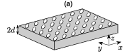
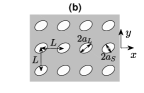
Figure 1: A PhC slab with a square lattice of elliptic air holes: (a) 3D view; (b) top view.

the structure is periodic in $x$ and $y$ with period $L$, the thickness of the slab is $2d=0.5L$, the semi-major and semi-minor axes of the elliptic air holes are $a_{L}$ and $a_{S}$, respectively, and the angle between the major axis and the $x$ axis is $\theta=\pi/6$. In addition, the dielectric constant of the PhC slab is $\varepsilon_{1}$ and the medium surrounding the PhC slab is air.

For $\varepsilon_{1}=4$, $a_{L}=0.3L$ and $a_{S}=0.2L$, the PhC slab has a few symmetry-protected BICs and a few propagating BICs. A particular TM-like propagating BIC, of which $E_{z}$ is odd in $z$ and $H_{z}$ is even in $z$, has a Bloch wavevector $(\alpha_{*},\beta_{*})=(-0.1515,0.2057)(2\pi/L)$ and a frequency $\omega_{*}=0.7017(2\pi c/L)$. In Figs. 2(a) and 2(b),

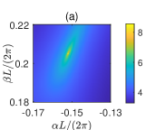
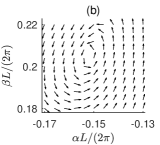
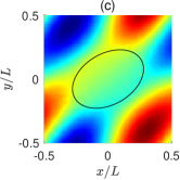
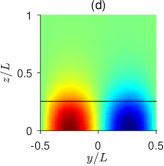
Figure 2: A BIC and its nearby resonant modes on a PhC slab with elliptic air holes ($\varepsilon_{1}=4$, $a_{L}=0.3L$, $a_{S}=0.2L$). (a) logrithmic value of the $Q$ factor, $\log_{10}Q$, of the resonant modes; (b) polarization direction of resonant modes; (c) and (d): the imaginary part of $H_{z}e^{-i(\alpha_{*}x+\beta_{*}y)}$ of the BIC on planes at $z=0$ and $x=0.5L$, respectively. Also shown in (c) and (d) are the boundary of the elliptic air hole and the horizontal slab-air interface.

we show the $Q$ factor and the polarization direction of the resonant modes near this BIC, i.e., for $(\alpha,\beta)$ near $(\alpha_{*},\beta_{*})$. The polarization direction of a resonant mode is the direction of the major axis of the polarization ellipse in the far field [22]. The BIC is the center of the polarization vortex in the $\alpha$-$\beta$ plane. As $(\alpha,\beta)$ traverses in the counterclockwise direction along a closed curve encircling $(\alpha_{*},\beta_{*})$, the continuously defined polarization direction accumulates a total angle of $2\pi$. Therefore, the topological charge of this BIC is $q=+1$ [22]. In Figs. 2(c) and 2(d), we show the imaginary part of $H_{z}e^{-i(\alpha_{*}x+\beta_{*}y)}$ on a horizontal plane at $z=0$ and a vertical plane at $x=0.5L$, respectively.

According to our theory, this propagating BIC is robust against structural perturbations satisfying the symmetry condition (2). Our numerical results confirm that the BIC exists as a continuous family when $\varepsilon_{1}$ and $a_{S}$ are varied. In Fig. 3,

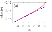
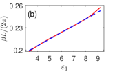
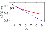
Figure 3: Bloch wavevector $(\alpha,\beta)$ and frequency $\omega$ of a propagating BIC for different values of $\varepsilon_{1}$. The red solid lines and the blue dashed lines are the direct numerical results and first order approximations, respectively.

we show $\alpha$, $\beta$ and $\omega$ of this BIC family as functions of $\varepsilon_{1}$ (solid red lines) for fixed $a_{L}=0.3L$ and $a_{S}=0.2L$. Useful approximations can be obtained by keeping only the first order terms in the perturbation theory. Assuming the unperturbed structure is the PhC slab with $\varepsilon_{1}=4$, then the perturbation of the dielectric function is $\delta s(\mathbf{x})$, where $\delta=\varepsilon_{1}-4$, $s(\mathbf{x})=1$ for $\mathbf{x}$ in the slab but outside the air holes and $s(\mathbf{x})=0$ otherwise. The first order perturbation terms can be calculated numerically, and they are $\alpha_{1}=0.0032(2\pi/L)$, $\beta_{1}=0.0091(2\pi/L)$, and $k_{1}=-0.0820(2\pi/L)$. In Fig. 3, the first order approximations, i.e., $\alpha\approx\alpha_{*}+\alpha_{1}(\varepsilon_{1}-4)$, $\beta\approx\beta_{*}+\beta_{1}(\varepsilon_{1}-4)$, and $k\approx k_{*}+k_{1}(\varepsilon_{1}-4)$, are shown as the blue dashed lines. The results are quite accurate for $\varepsilon_{1}$ near $4$. The propagating BIC also exists continuously with respect to $a_{L}$ and $a_{S}$. In Fig. 4,

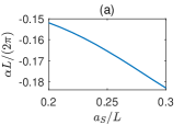
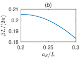
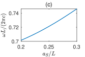
Figure 4: Bloch wavevector $(\alpha,\beta)$ and frequency $\omega$ of a propagating BIC for different values of $a_{S}$.

we show $\alpha$, $\beta$ and $\omega$ of this BIC family as continuous functions of $a_{S}$. These results are obtained for fixed $\varepsilon_{1}=4$ and $a_{L}=0.3L$.

VII Conclusion

For biperiodic structures with inversion and reflection symmetries, we showed that the low-frequency propagating BICs (with only one radiation channel) are robust against structural perturbations that preserve the same symmetries. The robustness is only conditional, since a BIC can be easily destroyed by a general perturbation. So far, we have assumed that both the original and the perturbed structure are lossless. It is not difficult to see that the result is still valid if the perturbation profile is symmetric in $z$ and $\mathcal{PT}$-symmetric in $x$ and $y$, i.e. $s(\mathbf{x})=s(x,y,-z)=\overline{s}(-x,-y,z)=\overline{s}(-\mathbf{x})$. A small material loss can also be considered as a perturbation. It is obvious that a lossy biperiodic structure cannot have a BIC with a real frequency and a real Bloch wavevector. It turns out that it usually cannot even have a bound state with a complex frequency and a real non-zero Bloch wavevector [24]. In other words, if the original lossless structure has a propagating BIC and the perturbation profile $s({\bf x})$ represents material loss and satisfies the symmetry condition (2), then a propagating BIC is usually destroyed by the perturbation.

The theory developed in this paper is applicable to symmetry-protected BICs, but the reflection symmetry in $z$ is not necessary. Assuming the biperiodic structure has only the inversion symmetry in the $xy$ plane, i.e. $\varepsilon({\bf x})=\varepsilon(-x,-y,z)$, a symmetry-protected BIC is a standing wave (with a zero Bloch wavevector) satisfying

$$E_{x}({\bf x}) = -E_{x}(-x,-y,z),\quad E_{y}({\bf x})=-E_{y}(-x,-y,z),$$

$$E_{z}({\bf x}) = E_{z}(-x,-y,z).$$

If we follow the scaling process of Sec. IV, then the electric field $E$ of the symmetry-protected BIC is pure imaginary. Meanwhile, we can construct two real diffraction solutions $U^{(1)}(\mathbf{x})$ and $U^{(2)}(\mathbf{x})$ for normal incident waves such that

$$U^{(l)}_{x}({\bf x}) = U^{(l)}_{x}(-x,-y,z),\quad U^{(l)}_{y}({\bf x})=U^{(l)}_{y}(-x,-y,z),$$

$$U^{(l)}_{z}({\bf x}) = -U^{(l)}_{z}(-x,-y,z)$$

for $l=1$ and 2. The perturbation process of Sec. V is still valid, provided that we replace $\Phi$, $\Psi_{e}$ and $\Theta_{e}$ by $E$, $U^{(1)}$ and $U^{(2)}$, respectively. In each step, we can show that $\alpha_{j}=\beta_{j}=0$, $k_{j}$ is real, and Eqs. (38) and (39) has a solution $\Phi_{j}$ that decays to zero exponentially as $|z|\to+\infty$ and satisfies the same symmetry condition as the BIC.

Finally, we point out that the justification for conditional robustness presented in this paper is still somewhat informal. It is desirable to develop a rigorous proof, including the convergence of the series (33) - (36), using a proper functional analysis framework.

Appendix A

To derive the first equation of the linear system (43), we take the dot product of $\overline{\Phi}$ with Eq. (38), integrate on domain $\Omega=\left\{(x,y,z)\,:\,|x|<L/2,\,|y|<L/2,\,|z|<+\infty\right\}$, and obtain

$$\int_{\Omega}\overline{\Phi}\cdot\mathcal{L}\Phi_{j}d{\bf x}=a_{11}\alpha_{j}+a_{12}\beta_{j}+a_{13}k_{j}-b_{1j}.$$ (61)

We need to show that the left hand side above is zero. Since $\mathcal{L}\Phi=0$, we have $\int_{\Omega}\Phi_{j}\cdot\overline{\mathcal{L}}\overline{\Phi}d{\bf x}=0$, and thus

$$\int_{\Omega}\overline{\Phi}\cdot\mathcal{L}\Phi_{j}d{\bf x}=\int_{\Omega}\overline{\Phi}\cdot\left(\nabla\times\nabla\times\Phi_{j}\right)d{\bf x}$$

$$+i\int_{\Omega}\overline{\Phi}\cdot\left[\nabla\times\left(\mathbf{b}\times\Phi_{j}\right)\right]d{\bf x}+i\int_{\Omega}\overline{\Phi}\cdot\left[\mathbf{b}\times\left(\nabla\times\Phi_{j}\right)\right]d{\bf x}$$

$$-\int_{\Omega}\overline{\Phi}\cdot\left[\mathbf{b}\times\left(\mathbf{b}\times\Phi_{j}\right)\right]d{\bf x}-\int_{\Omega}{\Phi_{j}}\cdot\left(\nabla\times\nabla\times\overline{\Phi}\right)d{\bf x}$$

$$+i\int_{\Omega}\Phi_{j}\cdot\left[\nabla\times\left(\mathbf{b}\times\overline{\Phi}\right)\right]d{\bf x}+i\int_{\Omega}\Phi_{j}\cdot\left[\mathbf{b}\times\left(\nabla\times\overline{\Phi}\right)\right]d{\bf x}$$

$$+\int_{\Omega}\Phi_{j}\cdot\left[\mathbf{b}\times\left(\mathbf{b}\times\overline{\Phi}\right)\right]d{\bf x}.$$ (62)

Using the vector identities

$$A\cdot\left(\nabla\times B\right)=B\cdot\left(\nabla\times A\right)+\nabla\cdot\left(B\times A\right),$$ (63)

$$A\cdot\left(B\times C\right)=B\cdot\left(C\times A\right)=C\cdot\left(A\times B\right)$$ (64)

in Eq. (Appendix A), we have

$$\int_{\Omega}\overline{\Phi}\cdot\mathcal{L}\Phi_{j}d{\bf x}=\int_{\Omega}\nabla\cdot\left[\left(\nabla\times\Phi_{j}\right)\times\overline{\Phi}\right]d{\bf x}$$

$$+i\int_{\Omega}\nabla\cdot\left[\left(\mathbf{b}\times\Phi_{j}\right)\times\overline{\Phi}\right]d{\bf x}-\int_{\Omega}\nabla\cdot\left[\left(\nabla\times\overline{\Phi}\right)\times\Phi_{j}\right]d{\bf x}$$

$$+i\int_{\Omega}\nabla\cdot\left[\left(\mathbf{b}\times\overline{\Phi}\right)\times\Phi_{j}\right]d{\bf x}.$$ (65)

Because of the Gauss’ Law, the above equation becomes

$$\int_{\Omega}\overline{\Phi}\cdot\mathcal{L}\Phi_{j}d{\bf x}=\int_{\partial\Omega}\left[\left(\nabla\times\Phi_{j}\right)\times\overline{\Phi}\right]\cdot d\mathbf{S}$$

$$+i\int_{\partial\Omega}\left[\left(\mathbf{b}\times\Phi_{j}\right)\times\overline{\Phi}\right]\cdot d\mathbf{S}-\int_{\partial\Omega}\left[\left(\nabla\times\overline{\Phi}\right)\times\Phi_{j}\right]\cdot d\mathbf{S}$$

$$+i\int_{\partial\Omega}\left[\left(\mathbf{b}\times\overline{\Phi}\right)\times\Phi_{j}\right]\cdot d\mathbf{S}.$$ (66)

Since $\Phi$ and $\Phi_{j}$ are periodic in the $x$ and $y$ directions, and $\Phi$ decays to zero exponentially as $|z|\to\infty$, the surface integrals above are zero. Therefore, $\int_{\Omega}\overline{\Phi}\cdot\mathcal{L}\Phi_{j}d{\bf x}=0$.

Since we assumed that $\Phi_{j}$ decays to zero exponentially as $|z|\to\infty$, $\overline{\Psi}_{e}\cdot{\cal L}\Phi_{j}$ and $\overline{\Theta}_{e}\cdot{\cal L}\Phi_{j}$ are also integrable on $\Omega$. Using the same steps above, it can be shown that their integrals are zero. This leads to the second and third equations in system (43).

Appendix B

Unlike the case considered in Appendix A, we only know $\Phi_{1}$ is outgoing as $z\to\pm\infty$. This implies that $\Phi_{1}$ is bounded at infinity, and we have to consider the integrals on a bounded domain $\Omega_{h}$ first. To derive Eq. (53), we note that $\mathcal{L}\Psi_{e}=0$. Therefore,

$$\int_{\Omega_{h}}\overline{\Psi}_{e}\cdot\mathcal{L}\Phi_{1}d{\bf x}=\int_{\Omega_{h}}\left(\overline{\Psi}_{e}\cdot\mathcal{L}\Phi_{1}-\Phi_{1}\cdot\overline{\mathcal{L}}\overline{\Psi}_{e}\right)d{\bf x}.$$

Using vector identities (63) and (64) and Gauss’ Law, we obtain

$$\int_{\Omega_{h}}\overline{\Psi}_{e}\cdot\mathcal{L}\Phi_{1}d{\bf x}$$

$$=\int_{\partial\Omega_{h}}\left[(\nabla\times\Phi_{1})\times\overline{\Psi}_{e}-(\nabla\times\overline{\Psi}_{e})\times\Phi_{1}\right]\cdot d\mathbf{S}$$

$$+\int_{\partial\Omega_{h}}i\left[(\mathbf{b}\times\Phi_{1})\times\overline{\Psi}_{e}+(\mathbf{b}\times\overline{\Psi}_{e})\times\Phi_{1}\right]\cdot d\mathbf{S}.$$

Since $\Phi_{1}$ and $\overline{\Psi}_{e}$ are periodic in the $x$ and $y$ directions, the integral on the surface parallel to the $z$-axis is zero. Thus

$$\int_{\Omega_{h}}\overline{\Psi}_{e}\cdot\mathcal{L}\Phi_{1}d{\bf x}=\int_{D_{xy}}\mathbf{e}_{3}\cdot\left[(\nabla\times\Phi_{1})\times\overline{\Psi}_{e}-(\nabla\times\overline{\Psi}_{e})\times\Phi_{1}\right]d{\rm r}$$

$$+i\int_{D_{xy}}\mathbf{e}_{3}\cdot\left[(\mathbf{b}\times\Phi_{1})\times\overline{\Psi}_{e}+(\mathbf{b}\times\overline{\Psi}_{e})\times\Phi_{1}\right]^{z=h}_{z=-h}d{\rm r},$$

where ${\rm r}=(x,y)$, $D_{xy}=\left\{(x,y)\,:\,|x|<L/2,\,|y|<L/2\right\}$, and $\mathbf{e}_{3}=(0,0,1)$ is the unit vector along the $z$ axis. Based in the asymptotic formulae (15) and (52), it is not difficult to show that

$$\lim\limits_{h\to+\infty}\int_{\Omega_{h}}\overline{\Psi}_{e}\cdot\mathcal{L}\Phi_{1}d{\bf x}=-2i\gamma L^{2}\left(\mathbf{c}^{+}\cdot\mathbf{d}^{+}+\mathbf{c}^{-}\cdot\mathbf{d}^{-}\right).$$

Noting that $\mathbf{c}^{-}\cdot\mathbf{d}^{-}=\mathbf{c}^{+}\cdot\mathbf{d}^{+}$, we obtain Eq. (53).

References

- [1] C. W. Hsu, B. Zhen, A. D. Stone, J. D. Joannopoulos, and M. Soljačić, “Bound states in the continuum,” Nat. Rev. Mater. 1, 16048 (2016).
- [2] K. Koshelev, G. Favraud, A. Bogdanov, Y. Kivshar, and A. Fratalocchi, “Nonradiating photonics with resonant dielectric nanostructures,” Nanophotonics 8, 725-745 (2019)
- [3] A.-S. Bonnet-Bendhia and F. Starling, “Guided waves by electromagnetic gratings and nonuniqueness examples for the diffraction problem,” Math. Methods Appl. Sci. 17, 305-338 (1994).
- [4] S. P. Shipman and S. Venakides, “Resonance and bound states in photonic crystal slabs,” SIAM J. Appl. Math. 64, 322-342 (2003).
- [5] P. Paddon and J. F. Young, “Two-dimensional vector-coupled-mode theory for textured planar waveguides,” Phys. Rev. B 61, 2090-2101 (2000).
- [6] T. Ochiai and K. Sakoda, “Dispersion relation and optical transmittance of a hexagonal photonic crystal slab,” Phys. Rev. B 63, 125107 (2001).
- [7] S. G. Tikhodeev, A. L. Yablonskii, E. A Muljarov, N. A. Gippius, and T. Ishihara, “Quasi-guided modes and optical properties of photonic crystal slabs,” Phys. Rev. B 66, 045102 (2002).
- [8] S. Shipman and D. Volkov, “Guided modes in periodic slabs: existence and nonexistence,” SIAM J. Appl. Math. 67, 687–713 (2007).
- [9] J. Lee, B. Zhen, S. L. Chua, W. Qiu, J. D. Joannopoulos, M. Soljačić, and O. Shapira, “Observation and differentiation of unique high-Q optical resonances near zero wave vector in macroscopic photonic crystal slabs,” Phys. Rev. Lett. 109, 067401 (2012).
- [10] Z. Hu and Y. Y. Lu, “Standing waves on two-dimensional periodic dielectric waveguides,” Journal of Optics 17, 065601 (2015).
- [11] R. Porter and D. Evans, “Embedded Rayleigh-Bloch surface waves along periodic rectangular arrays,” Wave Motion 43, 29-50 (2005).
- [12] D. C. Marinica, A. G. Borisov, and S. V. Shabanov, “Bound states in the continuum in photonics,” Phys. Rev. Lett. 100, 183902 (2008).
- [13] C. W. Hsu, B. Zhen, J. Lee, S.-L. Chua, S. G. Johnson, J. D. Joannopoulos, and M. Soljačić, “Observation of trapped light within the radiation continuum,” Nature 499, 188–191 (2013).
- [14] Y. Yang, C. Peng, Y. Liang, Z. Li, and S. Noda, “Analytical perspective for bound states in the continuum in photonic crystal slabs,” Phys. Rev. Lett. 113, 037401 (2014).
- [15] B. Zhen, C. W. Hsu, L. Lu, A. D. Stone, and M. Soljačič, “Topological nature of optical bound states in the continuum,” Phys. Rev. Lett. 113, 257401 (2014).
- [16] E. N. Bulgakov and A. F. Sadreev, “Bloch bound states in the radiation continuum in a periodic array of dielectric rods,” Phys. Rev. A 90, 053801 (2014).
- [17] R. Gansch, S. Kalchmair, P. Genevet, T. Zederbauer, H. Detz, A. M. Andrews, W. Schrenk, F. Capasso, M. Lončar, and G. Strasser, “Measurement of bound states in the continuum by a detector embedded in a photonic crystal,” Light: Science & Applications 5, e16147 (2016).
- [18] L. Li and H. Yin, “Bound states in the continuum in double layer structures,” Sci. Rep. 6, 26988 (2016).
- [19] L. Ni, Z. Wang, C. Peng, and Z. Li, “Tunable optical bound states in the continuum beyond in-plane symmetry protection,” Phys. Rev. B 94, 245148 (2016).
- [20] L. Yuan and Y. Y. Lu, “Propagating Bloch modes above the lightline on a periodic array of cylinders,” J. Phys. B: Atomic, Mol. and Opt. Phys. 50, 05LT01 (2017).
- [21] L. Yuan and Y. Y. Lu, “Bound states in the continuum on periodic structures: perturbation theory and robustness,” Optics Letters 42(21), 4490-4493 (2017).
- [22] E. N. Bulgakov and D. N. Makismov, “Bound states in the continuum and polarization singularities in periodic arrays of dielectric rods,” Phys. Rev. A 96, 063833 (2017).
- [23] J. Jin, X. Yin, L. Ni, M. Soljacic, B. Zhen, and C. Peng, “Topologically enabled unltrahigh- guided resonances robust to out-of-plane scattering,” Nature 574, 501-504 (2019).
- [24] Z. Hu, L. Yuan, and Y. Y. Lu, “Bound states with complex frequencies near the continuum on lossy periodic structures,” Phys. Rev. A 101, 013806 (2020).
- [25] L. Yuan and Y. Y. Lu, “Parametric dependence of bound states in the continuum on periodic structures,” Phys. Rev. A 102, 033513 (2020).
- [26] L. Yuan and Y. Y. Lu, “Bound states in the continuum on periodic structures surrounded by strong resonances,” Phys. Rev. A 97, 043828 (2018)
- [27] K. Koshelev, S. Lepeshov, M. Liu, A. Bogdanov, and Y. Kibshar, “Asymmetric metasurfaces with high- resonances governed by bound states in the contonuum,” Phys. Rev. Lett. 121, 193903 (2018)
- [28] Z. Hu and Y. Y. Lu, “Resonances and bound states in the continuum on periodic arrays of slightly noncircular cylinders,” J. Phys. B: At. Mol. Opt. Phys. 51, 035402 (2018).
- [29] L. Yuan and Y. Y. Lu, “Perturbation theories for symmetry-protected bound states in the continuum on two-dimensional periodic structures,” Phys. Rev. A 101, 043827 (2020).
- [30] A. Kodigala, T. Lepetit, Q. Gu, B. Bahari, Y. Fainman, and B. Kanté, “Lasing action from photonic bound states in continuum,” Nature 541, 196-199 (2017).
- [31] S. Romano, A. Lamberti, M. Masullo, E. Penzo, S. Cabrini, I. Rendina, and V. Mocella, “Optical biosensors based on photonic crystals supporting bound states in the continuum,” Materials 11, 526 (2018).
- [32] F. Yesilkoy, E. R. Arvelo, Y. Jahani, M. Liu, A. Tittl, V. Cevher, Y. Kivshar, and H. Altug, “Ultrasensitive hyperspectral imaging and biodetection enabled by dielectric metasurfaces,” Nature Photonics 13, 390-396 (2019).
- [33] J. M. Foley, S. M. Young, and J. D. Phillips, “Symmetry-protected mode coupling near normal incidence for narrow-band transmission filtering in a dielectric grating,” Phys. Rev. B 89, 165111 (2014).
- [34] X. Cui, H. Tian, Y. Du, G. Shi, and Z. Zhou, “Normal incidence filter using symmetry-protected modes in dielectric subwavelength gratings,” Sci. Rep. 6, 36066 (2016)
- [35] S. Han, L. Cong, Y. K. Srivastava, B. Qiang, M. V. Rybin, A. Kumar, R. Jain, W. X. Lim, V. G. Achanta, S. S. Prabhu, Q. J. Wang, Y. S. Kivshar, and R. Singh, “All-dielectric active terahertz photonics driven by bound states in the continuum,” Advanced Materials 31, 1901921 (2019).
- [36] L. Yuan and Y. Y. Lu, “Diffraction of plane waves by a periodic array of nonlinear circular cylinders,” Phys. Rev. A 94, 013852 (2016).
- [37] L. Yuan and Y. Y. Lu, “Strong resonances on periodic arrays of cylinders and optical bistability with weak incident waves,” Phys. Rev. A 95, 023834 (2017).
- [38] L. Yuan and Y. Y. Lu, “Excitation of bound states in the continuum via second harmonic generations,” SIAM J. Appl. Math. 80, 864-880 (2020).
- [39] K. Koshelev, S. Kruk, E. Melik-Gaykazyan J.-H. Choi, A. Bogdanov, H.-G. Park, Y. Kivshar, “Subwavelength dielectric resonators for nonlinear nanophotonics,” Science 367, 288-292 (2020).
- [40] W. Liu, B. Wang, Y. Zhang, J. Wang, M. Zhao, F. Guan, X. Liu, L. Shi, and J. Zi, “Circularly Polarized States Spawning from Bound States in the Continuum,” Phys. Rev. Lett. 123, 116104 (2019).
- [41] T. Yoda and M. Notomi, “Generation and Annihilation of Topologically Protected Bound States in the Continuum and Circularly Polarized States by Symmetry Breaking,” Phys. Rev. Lett. 125, 053902 (2020).
- [42] X. Yin, J. Jin, M. Soljačić, C. Peng, and B. Zhen, “Observation of topologically enabled unidirectional guided resonances,” Nature (London) 580, 467-471 (2020).