Reinforcement Learning via Parametric Cost Function Approximation for Multistage Stochastic Programming

Abstract: The most common approaches for solving stochastic resource allocation problems in the research literature is to either use value functions (“dynamic programming”) or scenario trees (“stochastic programming”) to approximate the impact of a decision now on the future. By contrast, common industry practice is to use a deterministic approximation of the future which is easier to understand and solve, but which is criticized for ignoring uncertainty. We show that a parameterized version of a deterministic lookahead can be an effective way of handling uncertainty, while enjoying the computational simplicity of a deterministic lookahead. We present the parameterized lookahead model as a form of policy for solving a stochastic base model, which is used as the basis for optimizing the parameterized policy. This approach can handle complex, high-dimensional state variables, and avoids the usual approximations associated with scenario trees. We formalize this approach and demonstrate its use in the context of a complex, nonstationary energy storage problem.

Keywords: Stochastic Optimization, Policy Search, Stochastic Programming, Simulation-based Optimization, Parametric Cost Function Approximation

1 Introduction

There has been a long history in industry of using deterministic optimization models to make decisions that are then implemented in a stochastic setting. Energy companies use deterministic forecasts of wind, solar and loads to plan energy generation (Wallace and Fleten (2003)); airlines use deterministic estimates of flight times to schedule aircraft and crews (Lan et al. (2006)); and retailers use deterministic estimates of demands and travel times to plan inventories (Harrison and Van Mieghem (1999)). These models have been widely criticized in the research community for not accounting for uncertainty, which often motivates the use of large-scale stochastic programming models which explicitly model uncertainty in future outcomes (Mulvey et al. (1995) and Birge and Louveaux (2011)). These large-scale stochastic programs, which use scenario trees to approximate future events, have been applied to unit commitment (Jin et al. (2011)), hydroelectric planning (Carpentier et al. (2015)), and transportation (Lium et al. (2009)). These models are computationally very demanding, yet still require a number of approximations and, as a result do not produce optimal policies.

We make the case that these previous approaches ignore the true problem that is being solved, which is always stochastic. The so-called “deterministic models” used in industry are almost always parametrically modified deterministic approximations, where the modifications are designed to handle uncertainty. Both the “deterministic models” and the “stochastic models” (formulated using the framework of stochastic programming) are examples of lookahead policies to solve a stochastic optimization problem with the goal of finding the best policy which is typically tested using a simulator, but which may be field tested in an online environment (the real world).

In this paper, we characterize these modified deterministic models as parametric cost function approximations (CFAs) which puts them into the same category as other parameterized policies that are well known in the research community working on policy search (Ng and Jordan (2000), Peshkin et al. (2000), Hu et al. (2007), Deisenroth et al. (2013), and Mannor et al. (2003)). A parallel community has evolved under the name simulation-optimization (see the recent edited volume Fu (2015)), where powerful tools have been developed based on the idea of taking derivatives of simulations (see the extensive literature on derivatives of simulations covered in Glasserman (1991), Ho (1992), Kushner and Yin (2003), Cao (2008)); a nice tutorial is given in Chau et al. (2014). Much of this literature focuses on derivatives of discrete event simulations with respect to static parameters such as a buffer stock. Our problem also exhibits static parameters, but in the form of parameterized modifications of constraints in a policy that involves solving a linear program.

Our use of modified linear programs is new to the policy search literature, where “policies” are typically parametric models such as linear models (“affine policies”), structured nonlinear models (such as (s,S) policies for inventories) or neural networks (Han and E (2016)). There are two dimensions to our approach: the design of the parameterized lookahead model, and the optimization of the parameters so that a particular parameterization performs as well as it can. The process of designing the modifications (in this paper, these modifications always appear in the constraints) requires the same art as the design of any statistical model or parametric policy, a process that requires exploiting the structure of the problem. This paper addresses the second dimension, which is the design of gradient-based search algorithms which are nontrivial in this setting.

This paper formalizes the idea, used for years in industry, that an effective way to solve complex stochastic optimization problems is to shift the modeling of uncertainty from a lookahead approximation, where even deterministic lookahead models can be hard to solve, to the stochastic base model, typically implemented as a simulator but which might also be the real world. Tuning a model in a stochastic simulator makes it possible to handle arbitrarily complex dynamics, avoiding the many approximations (such as two-stage models, scenario trees, exogenous information that is independent of decisions) that are standard in stochastic programming. In the process, we are expanding the range of problems considered by the simulation-optimization community to the entire class of vector-valued multistage stochastic optimization problems considered in the stochastic programming literature.

The CFAs make it possible to exploit structural properties. For example, it may be obvious that the way to handle uncertainty when planning energy generators in a unit commitment problem is to require extra reserves at all times of the day. A stochastic programming model encourages this behavior, but the requirement for a manageable number of scenarios will produce the required reserve only when one of the scenarios requires it. In addition, the almost universal use of two-stage approximations (where the future is modeled as a single stage, which means that decisions in the future are allowed to see into the future) underestimates the effect of uncertainty in the future. Imposing a reserve constraint (which is a kind of cost function approximation) allows us to impose the aforementioned requirement at all times of the day, and to tune it under very realistic conditions without any of the approximations required by stochastic programs.

Designing a parametric CFA closely parallels the design of any parametric statistical model, which is part art (creating the model) and part science (fitting the model). In fact, the design of the parameterization and the tuning of the parameters each represent important areas of research. Most important, the parametric CFA opens up a fundamentally new approach for providing practical tools for solving high-dimensional, stochastic programming problems. It provides an alternative to classical stochastic programming with its focus on optimizing a stochastic lookahead model which requires a variety of approximations to make it computationally tractable (and even then, it is typically computationally very demanding).

The parametric CFA makes it possible to incorporate problem structure for handling uncertainty. Some examples include: supply chains handle uncertainty by introducing buffer stocks; hospitals can handle uncertainty in blood donations and the demand for blood by maintaining supplies of O-minus blood, which can be used by anyone; and grid operators handle uncertainty in generator failures, as well as uncertainty in energy from wind and solar, by requiring generating reserves. Central to our approach is the ability to manage uncertainty by recognizing effective strategies for responding to unexpected events. We would argue that this structure is apparent in many settings, especially in complex resource allocation problems. At a minimum, we offer that our approach represents an interesting, and very practical, alternative to stochastic programming.

This paper makes the following contributions. First, we introduce and develop the idea of parameterized cost function approximation as a tool for solving important classes of multistage stochastic programming problems, shifting the focus from solving complex, stochastic lookahead models to optimizing a stochastic base model. This approach is computationally comparable to solving deterministic approximations, with the exception that the parametric modifications have to be optimized, typically in a simulator that avoids the many approximations made in stochastic lookahead models. To the best of our knowledge, this is the first fundamentally new approach for solving the aforementioned class of stochastic optimization problems which is as easy to compute as a deterministic lookahead.

Second, we provide some theoretical results about the structure of the objective function and the optimal policy of our optimization problem in the CFA approach. In particular, we show that while the objective function is generally nonconvex, it admits special structure under different types of parameterization policies.

Third, we propose a simulation-based optimization algorithm and establish its finite-time rate of covergence for performing the policy search in our nonconvex stochastic optimization problem. Since this algorithm only uses noisy objective values, it gives us more flexibility in choosing the parametric model for the CFA approach.

Finally, we specialize our CFA approach for a complex, nonstationary energy storage problem in the presence of rolling forecasts. Our numerical experiments demonstrate that while our optimization problem is nonconvex, our proposed algorithm, regardless of the quality of the starting point, can find a parameterization policy whose performance is significantly better than a base policy using unmodified rolling forecasts.

Our presentation is organized as follows. The modeling framework and an overview of the different classes of policies are given in Section 2. We then formally introduce the parametric CFA approach in Section 3. Algorithms for optimizing policy parameters together with their convergence properties and some theoretical results about structure of the optimization problem in the CFA approach are presented in Section 4. We then specialize the parametric CFA approach for an energy storage application and present some numerical experiments for solving this problem in Section 5. Finally, we conclude the paper in Section 6.

2 Canonical Model and Solution Strategies

Our main problem of interest in this paper is to find a policy $\pi$ that solves

$$\min_{\pi\in\Pi}\>\>\mathbb{E}^{\pi}\bigg{[}\sum^{T}_{t=0}C_{t}(S_{t},X^{\pi}_{t}(S_{t}))\>\bigg{|}\>S_{0}\bigg{]},$$ (1)

where $S_{t+1}=S^{M}(S_{t},X^{\pi}_{t}(S_{t}),W_{t+1})$. Here, $\Pi$ denotes the set of all possible policies, $S_{t}$ represents the sate variable, and $X^{\pi}_{t}(S_{t})$ denotes the decision function (policy) which determines decision variable $x_{t}\in\mathcal{X}_{t}\subseteq\mathbb{R}^{n}$. Furthermore, $W_{t+1}$ denotes exogenous information which describes the information that first becomes known at time $t+1$ which may depend on the state $S_{t}$ and/or the action $x_{t}$, and $S^{M}(\cdot)$ denotes the transition function which explicitly describes the relationship between the state of the model at time $t$ and $t+1$. We state this canonical model because it sets up our modeling framework, which is fundamentally different than the standard paradigm of stochastic programming (for multistage problems). However, it sets the foundation for searching over policies which is fundamental to our approach. We refer interested readers to Powell (2011) for more detailed explanation of these elements of sequential stochastic decision problems.

In the rest of this section, we describe the major classes of policies that we can draw from to solve problem (1). There are two fundamental strategies for designing policies. The first is policy search, where we search over different classes of functions $f\in{\cal F}$ and different parameters $\theta^{f}\in\Theta^{f}$ in each class. Policy search is written as

$$\min_{\pi=(f,\theta^{f})\in({\cal F},\Theta^{f})}{\mathbb{E}}\left\{\sum_{t=0}^{T}C_{t}(S_{t},X^{\pi}_{t}(S_{t}|\theta^{f}))\big{|}S_{0}\right\}.$$

Policies that can be identified using policy search come in two classes. The first one is policy function approximations (PFAs) including linear or nonlinear models, neural networks, and locally parametric functions. PFAs (using any of a wide range of approximation strategies) have been widely studied in the computer science literature under the umbrella of policy search (see e.g., Sutton et al. (1999), Bertsimas and Goyal (2012), Hadjiyiannis et al. (2011), Bertsimas et al. (2011), Lillicrap et al. (2015), Levine and Abbeel (2014). The second one is cost function approximations (CFAs). In this approach, we use parametrically modified costs and constraints that are then minimized. These are written as

$$X^{CFA}(S_{t}|\theta)={\rm argmin}_{x_{t}\in{\cal X}^{\pi}(\theta)}{\bar{C}}^{\pi}(S_{t},x_{t}|\theta),$$

where ${\bar{C}}^{\pi}(S_{t},x_{t}|\theta)$ and ${\cal X}^{\pi}(\theta)$ are parametrically modified cost function and set of constraints. CFAs are widely used in industry for complex problems such as scheduling energy generation or planning supply chains, but they have not been studied formally in the research literature.

The second strategy is to construct policies based on lookahead models, where we capture the value of the downstream impact of a decision $x_{t}$ made while in state $S_{t}$. An optimal policy can be written

$$X^{*}_{t}(S_{t})={\rm argmin}_{x_{t}\in{\cal X}_{t}}\left(C_{t}(S_{t},x_{t})+{\mathbb{E}}\left\{\min_{\pi\in\Pi}{\mathbb{E}}\left\{\sum_{t^{\prime}=t+1}^{T}C_{t^{\prime}}(S_{t^{\prime}},X^{\pi}_{t^{\prime}}(S_{t^{\prime}}))\big{|}S_{t+1}\right\}\big{|}S_{t},x_{t}\right\}\right).$$ (2)

Equation (2) is basically Bellman’s equation, but it is computable only for very special instances. Two core strategies for approximating the lookahead portion in (2) include value function approximations (see e.g., Powell (2011), Bertsekas (2011), Sutton and Barto (2018), Powell et al. (2004)) and direct lookahead approximations (see e.g., (Sethi and Sorger 1991, Camacho and Alba 2013, Birge and Louveaux 2011, Donohue and Birge 2006)). In the former, we approximate the lookahead portion using a value function. When the lookahead problem cannot be reasonably approximated by a value function, the latter can be used to replace the model with an approximation for the purpose of approximating the future.

Policy search, whether we are using PFAs or CFAs, requires tuning parameters in our base objective function (1). By contrast, policies based on lookahead approximations depend on developing the best approximation of the future that can be handled computationally, although these still need to be evaluated using (1).

An often overlooked challenge is the presence of forecasts. These inherently require some form of lookahead, but are universally ignored when using value function approximations (the forecast would be part of the state variable). However, stochastic lookahead approximations are typically computationally very demanding. In this paper, we are going to propose a hybrid comprised of a deterministic lookahead which is modified with parameters that have to be tuned using policy search. This idea has been widely used in industry in an ad-hoc fashion without formal tuning of the parameters. We develop this idea in the context of a multistage linear program using the context of a complex, time-dependent energy storage problem with time-varying forecasts.

3 The Parametric Cost Function Approximations

We extend the concept of policy search to include parameterized optimization problems. The CFA draws on the structural simplicity of deterministic lookahead models and myopic policies, but allows more flexibility by adding tunable parameters. This puts this methodology in the same class as parametric policy function approximations widely used in the policy search literature, with the only difference that our parameterized functions are inside an optimization problem, making them more useful for high dimensional problems.

3.1 Basic Idea

Since the idea of a parametric CFA is new, we begin by outlining the general strategy and then demonstrate how to apply it for our energy storage problem in Section 5. For our work, we only consider parameterizing the constraints which can be written as

$$X^{\pi}_{t}(S_{t}|\theta)={\rm argmin}_{x_{t}\in\mathcal{X}_{t}}\>\>C_{t}(S_{t},x_{t}),\qquad\text{s.t.}\qquad A_{t}x_{t}\leq b_{t}+D\theta^{b},$$ (3)

where $\theta^{b}$ is the vector of constraint parameters and $D$ is a scaling matrix. While the parametric terms can also be added to the cost function, we only consider parameterization of the constraints for our energy storage application in Section 5.

Whether the parameterizations are in the objective function, or in the constraints, the specification of a parametric CFA parallels the specification of any statistical model (or policy). The structure of the model is the “art” that draws on the knowledge and insights of the modeler. Finding the best CFA, which involves finding the best $\theta$, is the science which draws on the power of classical search algorithms. This paper focuses on designing algorithms for finding $\theta$ for a given parameterization.

3.2 A hybrid Lookahead-CFA policy

There are many problems that naturally lend themselves to a lookahead policy (for example, to incorporate a forecast or to produce a plan over time), but where there is interest in making the policy more robust than a pure deterministic lookahead using point forecasts. For this important class, we can create a hybrid policy where a deterministic lookahead has parametric modifications that have to be tuned using policy search. When parameters are applied to the constraints it is possible to incorporate easily recognizable problem structure. For example, a supply chain management problem can handle uncertainty through buffer stocks, while an airline scheduling model might handle stochastic delays using schedule slack. A grid operator planning energy generation in the future might schedule reserve capacity to account for uncertainty in forecasts of demand, as well as energy from wind and solar. As with all policy search procedures, there is no guarantee that the resulting policy will be optimal unless the parameterized space of policies includes the optimal policy. However, we can find the optimal policy within the parameterized class, which may reflect operational limitations. We note that while parametric CFAs are widely used in industry, optimizing within the parametric class is not done.

3.3 Structure of the cost function approximation

Assume that a lookahead policy is given as

$$X^{\text{D-LA}}_{t}(S_{t})={\rm argmin}_{x_{t},(\tilde{x}_{t,t^{\prime}},t^{\prime}=t+1,\ldots,\bar{T})}\>\>\left(c_{t}x_{t}+\>\sum^{\bar{T}}_{t^{\prime}=t+1}\tilde{c}_{t,t^{\prime}}\tilde{x}_{t,t^{\prime}}\right),$$ (4)

where $\bar{T}=\min(t+H,T)$, $\tilde{S}_{t,t^{\prime}+1}=\tilde{S}^{M}(\tilde{S}_{t,t^{\prime}},\tilde{x}_{t,t^{\prime}},\tilde{W}_{t,t^{\prime}+1})$, and $H$ is the size of the lookahead horizon. If the cost function, transition function, and constraints of $X^{\pi}(\cdot)$ are all linear, this policy can be expressed as the following linear program

$$X^{\text{D-LA}}_{t}(S_{t})={\rm argmin}_{x_{t},\tilde{x}_{t,t^{\prime}},t^{\prime}=t+1,\bar{T}}\left\{c_{t}x_{t}+\tilde{c}_{t}\tilde{x}_{t}:A_{t}x_{t}\leq b_{t},\>\tilde{A}_{t}\tilde{x}_{t}\leq\tilde{b}_{t},\>\>x_{t},\tilde{x}_{t}\geq 0\right\},$$

where $\tilde{a}_{t}=\{\tilde{a}_{t,t^{\prime}}\>:\>t^{\prime}=t+1,...,\bar{T}\}$ for any vector/matrix $\tilde{a}_{t,t^{\prime}}$. Parametric terms can be appended to the cost function and existing constraints, and new ones can also be added to the existing model. Often the problem setting will influence how the policy should be parameterized. In particular, there are different ways to parameterize the above-mentioned policy including parameterizing the cost vector, the A-matrix, and the right hand side vector. In particular, assuming that all the uncertainty is restricted to the right hand side constraints, we can parameterize the vector $b_{t}$ such that the parameterized policy becomes

$$X^{\text{LA-CFA}}_{t}(S_{t}|\theta)={\rm argmin}_{x_{t},\tilde{x}_{t,t^{\prime}},t^{\prime}=t+1,\bar{T}}\left\{c_{t}x_{t}+\tilde{c}_{t}\tilde{x}_{t}:A_{t}x_{t}\leq b_{t}(\theta),\>\tilde{A}_{t}\tilde{x}_{t}\leq\tilde{b}_{t}(\theta),\>\>x_{t},\tilde{x}_{t}\geq 0\right\},$$

where $\theta$ is a vector of tunable parameters. Parametric modifications can be designed specifically to capture the structure of a particular policy. For storage problems, the idea of using buffers and inventory constraints to manage storage is intuitive and easily incorporated into a deterministic lookahead. In particular, a lower buffer guarantees the decision maker will always have access to some stored quantities. Conversely, an upper threshold will make sure some storage space remains available for unexpected orders. Hence, representing the approximated future storage level at time $t^{\prime}$ given the information available at time $t$ by $R_{t,t^{\prime}}$, we can have $\theta^{L}\leq R_{t,t^{\prime}}\leq\theta^{U}\text{ for }t^{\prime}>t$. Although it can greatly increase the parameter space, the upper and lower bounds can also depend on $t^{\prime}-t$, as in

$$\theta^{L}_{t^{\prime}-t}\leq R_{t,t^{\prime}}\leq\theta^{U}_{t^{\prime}-t}\text{ for }t^{\prime}>t.$$ (5)

The resulting modified deterministic problem is no harder to solve than the original deterministic problem (where $\theta^{L}=0$ and $\theta^{U}=R^{max}$). We now have to use stochastic search techniques to solve the policy search problem to optimize $\theta$.

There are also different policies for parameterizing the right hand side adjustment. A simple form is a lookup table indexed by $t^{\prime}-t$ as in equation (5). Although it may be simple, a lookup table model for $\theta$ means that the dimensionality increases with the horizon which can complicate the policy search process. This type of parameterization is not limited to just modifying the point estimate of exogenous information. If the modeler has sufficient information such as the cumulative distribution function, one can even exchange the point estimate with the quantile function. The lookup table in time parameterization is best if the relationship between parameters in different periods is unknown.

Instead of having an adjustment $\theta_{\tau}=\theta_{t^{\prime}-t}$ for each time $t+\tau$ in the future, one can use instead a parametric function of $\tau$, which reduces the number of parameters that we have to estimate. For example, we might use the parametric adjustment given by

$$\theta_{1}^{L}\cdot e^{\tau\theta_{2}^{L}}\leq R_{t,t^{\prime}}\leq\theta_{1}^{U}\cdot e^{\tau\theta_{2}^{U}}\text{ for }t^{\prime}>t.$$

These parametric functions of time can also be used to directly modify the approximated future in the lookahead model.

We should point out that the parameterization scheme can be more general to better capture the underlying uncertainty in the model. In particular, one can also use the parameterized forms of $b(\theta(\sigma))$, $c(\theta(\sigma))$, $A(\theta(\sigma))$, where $\sigma$ represents an estimated variance of noise corresponding to the all sources of uncertainty. We let $\sigma=0$ correspond to the case of having perfect information about the future over the horizon, which is the same as assuming that the base model is deterministic. In this case, the parameterized model should satisfy $b_{t}(\theta(0))=b_{t}$, $c_{t}(\theta(0))=c_{t}$, $A_{t}(\theta(0))=A_{t}$. An important example of parameterization would be affine with the general form of $b_{t}(\theta)=\theta^{b}_{0}+\theta^{b}_{1}b_{t}$ (with similar modifications for the elements of the matrix A and the cost vector c). If $\sigma=0$, we would use $\theta^{b}_{0}=0$ and $\theta^{b}_{1}=1$. Finding the proper choice of parameterization is an art of modeling the problem which represents its own research challenges within the CFA approach and is beyond the scope of this paper.

4 Optimizing the parameters of the CFA model

To tune our parameterized policy in the CFA model, we need to solve

$$\min_{\theta\in\Theta}\>\left\{F(\theta):=\mathbb{E}_{\omega}\left[\bar{F}(\theta,\omega)\right]=\mathbb{E}\left[\sum_{t=0}^{T}C_{t}\bigg{(}S_{t}(\omega),X^{\pi}_{t}(S_{t}(\omega),\theta)\bigg{)}\bigg{|}S_{0}\right]\right\},$$ (6)

where $S_{t+1}(\omega)=S^{M}(S_{t}(\omega),X^{\pi}_{t}(S_{t}(\omega),\theta),W_{t+1}(\omega))$ for every $\omega\in\Omega$. If $F(\theta)$ is well-defined, finite-valued, convex, and continuous at every $\theta$ in the nonempty, closed, and convex set $\Theta\subset\mathbb{R}^{n}$, then an optimal $\theta^{*}\in\Theta$ exists and can be found by stochastic approximation (SA) algorithms. However, when $F(\theta)$ is possibly nonconvex, SA-type methods can be modified to find stationary points of the above problem. In Subsection 4.1, we propose the classical SA algorithm and discuss its convergence properties when a noisy gradient of the objective function in (6) is available. We then provide a randomized SA algorithm in Subsection 4.1 which only requires noisy observations of the objective function.

4.1 Stochastic Gradient method for optimizing the CFA model

Our goal in this subsection is to solve problem (6) under specific assumptions on $F(\theta)$. Stochastic approximation algorithms require computing stochastic (sub)gradients of the objective function iteratively. Due to the special structure of $F(\theta)$, its (sub)gradient can be computed recursively under certain conditions as shown in the next result.

Proposition 4.1

Assume $\bar{F}(\cdot,\omega)$ is convex/concave for every $\omega\in\Omega$, $\theta$ is an interior point of $\Theta$, and $F(\cdot)$ is finite valued in the neighborhood of $\theta$. If distribution of $\omega$ is independent of $\theta$, we have

$$\nabla_{\theta}F(\theta)=\mathbb{E}[\nabla_{\theta}\bar{F}(\theta,\omega)],$$

where

$$\nabla_{\theta}\bar{F}(\theta)=\bigg{(}\frac{\partial C_{0}}{\partial X^{\pi}_{0}}\cdot\frac{\partial X^{\pi}_{0}}{\partial\theta}\bigg{)}+\sum^{T}_{t=1}\bigg{[}\bigg{(}\frac{\partial C_{t}}{\partial S_{t}}\cdot\frac{\partial S_{t}}{\partial\theta}\bigg{)}+\bigg{(}\frac{\partial C_{t}}{\partial X^{\pi}_{t}}\cdot\bigg{(}\frac{\partial X^{\pi}_{t}}{\partial S_{t}}\cdot\frac{\partial S_{t}}{\partial\theta}+\frac{\partial X^{\pi}_{t}}{\partial\theta}\bigg{)}\bigg{)}\bigg{]},\\$$ (7)

$$\text{and}\qquad\frac{\partial S_{t}}{\partial\theta}=\frac{\partial S_{t}}{\partial S_{t-1}}\cdot\frac{\partial S_{t-1}}{\partial\theta}+\frac{\partial S_{t}}{\partial X^{\pi}_{t-1}}\cdot\bigg{[}\frac{\partial X^{\pi}_{t-1}}{\partial S_{t-1}}\cdot\frac{\partial S_{t-1}}{\partial\theta}+\frac{\partial X^{\pi}_{t-1}}{\partial\theta}\bigg{]},$$

in which the $\omega$ is dropped for simplicity.

Proof. If $\bar{F}(\cdot,\omega)$ is convex or concave for every $\omega\in\Omega$, $\theta$ is an interior point of $\Theta$, and $F(\cdot)$ is finite valued in the neighborhood of $\theta$, then we have $\nabla_{\theta}\left(\mathbb{E}\left[\bar{F}(\theta,\omega)\right]\right)=\mathbb{E}\left[\nabla_{\theta}\bar{F}(\theta,\omega)\right]$ by Strassen (1965). Applying the chain rule, we find

$$\begin{split}\nabla_{\theta}\bar{F}(\theta)&=\frac{d}{d\theta}\bigg{[}C_{0}(S_{0},X^{\pi}_{0})+\sum^{T}_{t=1}C(S_{t},X^{\pi}_{t})\bigg{]}=\bigg{(}\frac{\partial C_{0}}{dX^{\pi}_{0}}\cdot\frac{dX^{\pi}_{0}}{\partial\theta}\bigg{)}+\bigg{[}\sum^{T}_{t=1}\frac{d}{d\theta}\>C(S_{t},X^{\pi}_{t})\bigg{]}\\ &=\bigg{(}\frac{\partial C_{0}}{dX^{\pi}_{0}}\cdot\frac{dX^{\pi}_{0}}{\partial\theta}\bigg{)}+\sum^{T}_{t=1}\bigg{[}\bigg{(}\frac{\partial C_{t}}{\partial S_{t}}\cdot\frac{\partial S_{t}}{\partial\theta}\bigg{)}+\bigg{(}\frac{\partial C_{t}}{\partial X^{\pi}_{t}}\cdot\frac{dX^{\pi}_{t}}{d\theta}\bigg{)}\bigg{]}\\ &=\bigg{(}\frac{\partial C_{0}}{dX^{\pi}_{0}}\cdot\frac{dX^{\pi}_{0}}{\partial\theta}\bigg{)}+\sum^{T}_{t=1}\bigg{[}\bigg{(}\frac{\partial C_{t}}{\partial S_{t}}\cdot\frac{\partial S_{t}}{\partial\theta}\bigg{)}+\bigg{(}\frac{\partial C_{t}}{\partial X^{\pi}_{t}}\cdot\bigg{(}\frac{\partial X^{\pi}_{t}}{\partial S_{t}}\cdot\frac{\partial S_{t}}{\partial\theta}+\frac{\partial X^{\pi}_{t}}{\partial\theta}\bigg{)}\bigg{)}\bigg{]},\\ \end{split}$$

where $\tfrac{\partial S_{t}}{\partial\theta}=\tfrac{\partial S_{t}}{\partial S_{t-1}}\cdot\tfrac{\partial S_{t-1}}{\partial\theta}+\tfrac{\partial S_{t}}{\partial X^{\pi}_{t-1}}\big{[}\tfrac{\partial X^{\pi}_{t-1}}{\partial S_{t-1}}\cdot\tfrac{\partial S_{t-1}}{\partial\theta}+\tfrac{\partial X^{\pi}_{t-1}}{\partial\theta}\big{]}$.    

Note that if $\bar{F}(\theta)$ is not differentiable, then its subgradient can be still computed using (7). However, when $\bar{F}(\theta)$ is not convex (concave), its subgradient may not exist and the concept of generalized subgradient should be employed.

If $\nabla_{\theta}\bar{F}(\theta,\omega)$ exists for every $\omega\in\Omega$, the ability to calculate its unbiased estimator allows us to use stochastic approximation techniques to determine the optimal parameters, $\theta^{*}$, of the CFA policy model. Below is an iterative SA algorithm for optimizing the CFA model.

Algorithm 1 The stochastic gradient method for the CFA model (SG-CFA)

1:  Input: $\theta^{0}$, $N$.For $n=1,2,\ldots,N$:

2:  Generate a trajectory $\omega^{n}$ where

$$S^{n}_{t+1}(\omega^{n})=S^{M}(S^{n}_{t}(\omega^{n}),X_{t}^{\pi}(S^{n}_{t}(\omega^{n}),\theta^{n-1}),W_{t+1}(\omega^{n}))\qquad t=0,1,\ldots,T-1,$$

3:  Compute the gradient estimator using equation (7).

4:  Update policy parameters as

$$\theta^{n}=\theta^{n-1}-\alpha_{n-1}\nabla_{\theta}\bar{F}(\theta^{n-1},\omega^{n})|_{\theta=\theta^{n-1}}$$ (8)

End For

For the convergence of the above algorithm, we need to assume the following conditions (Robbins and Monro (1951)):

• The stochastic subgradient $g^{n}$ computed at the $n$-th iteration satisfies
  $\mathbb{E}\bigg{[}g^{n+1}({\theta}^{n}-\theta^{*})\bigg{|}\mathcal{F}^{n}\bigg{]}\leq 0$, and $\|g^{n}\|\leq B_{g}$ a.s.,

• For any $\theta$ where $|\theta-\theta^{*}|>\delta>0$, there exists $\epsilon>0$ such that $\|\mathbb{E}[g^{n+1}|\mathcal{F}^{n}]\|>\epsilon$.

Furthermore, we need to assume that stepsizes $\alpha_{n}$ satisfy

$$\alpha_{n}>0\>\>\text{a.s.},\qquad\qquad\sum^{\infty}_{n=0}\alpha_{n}=\infty\>\>\text{a.s.},\qquad\qquad{\mathbb{E}}\left[\sum^{\infty}_{n=0}\alpha^{2}_{n}\right]<\infty.$$ (9)

If the above conditions hold, $F(\cdot)$ is continuous and finite valued in the neighborhood of every $\theta$, in the nonempty, closed, bounded, and convex set $\Theta\subset\mathbb{R}^{d}$ such that $\bar{F}(\cdot,\omega)$ is convex for every $\omega\in\Omega$ where $\theta$ is an interior point of $\Theta$, then $\lim_{n\rightarrow\infty}\>\theta^{n}\longrightarrow\theta^{*}\>\>\text{a.s}$. Although any stepsize rule that satisfies the previous conditions will guarantee asymptotic convergence, we prefer parameterized rules that can be tuned for quicker convergence rates. Therefore, we limit our evaluation of the algorithm to how well it does within $N$ iterations. The CFA Algorithm can be described as a policy, $\theta^{\pi}(S^{n})$, with a state variable, $S^{n}=\theta^{n}$ plus any parameters needed to compute the stepsize policy, and where $\pi$ describes the structure of the stepsize rule. If $\theta^{\pi,n}$ is the estimate of $\theta$ using stepsize rule $\pi$ after $n$ iterations, then our goal is to find the rule that produces the best performance (in expectation) after we have exhausted our budget of $N$ iterations. Thus, we wish to solve $\min_{\pi}\mathbb{E}\left[\bar{F}(\theta^{\pi,N},\omega)\right]$ i.e., finding the best stepsize rule that minimizes the terminal cost within $N$ iterations. For our numerical experiments, we use two well-known stepsize policies, namely, the adaptive gradient algorithm (AdaGrad) Duchi et al. (2011) and the Root Mean Square Propagation (RMSProp) Tieleman and Hinton (2012), shown to perform well in practice. In particular, the AdaGrad modifies the individual stepsize for each coordinate of the updated parameter, $\theta$, based on previously observed stochastic gradients using

$$\alpha_{n,j}=\frac{\eta}{\sqrt{G_{n}(j,j)+\epsilon}},\ \ j=1,\ldots,d,$$

where $\eta>0$ is a scalar learning rate, $G_{n}\in\mathbb{R}^{d\times d}$ is a diagonal matrix where each diagonal element is the sum of the squares of the stochastic gradients with respect to $\theta$ up to the current iteration $n$, and $\epsilon>0$ avoids division by zero. On the other hand, the RMSProp uses a scaler stepsize based on a running average of previously observed stochastic gradients to scale the current stepsize as

$$\alpha_{n}=\frac{\eta}{\sqrt{\bar{g}^{n}}},\qquad\bar{g}_{n}=\beta\bar{g}^{n-1}+(1-\beta)\|g^{n}\|^{2},$$

where $\eta$ is the learning rate and $\beta\in(0,1)$ is the running weight.

Note that $F(\theta)$ can be generally nonsmooth and nonconvex and hence, its subgradient does not exist everywhere. While one can define generalized subgradients for this function, one can also define a smooth approximation of $F(\theta)$ and then try to apply a stochastic approximation algorithm to minimize this function. We pursue this idea in the next subsection.

4.2 Stochastic Gradient-free method for optimizing the CFA model

As mentioned in the previous subsection, the gradient of $F(\theta)$ in (7) is only computable under restricted conditions. However, noisy values of $F(\theta)$ can be obtained through simulation. This motivates using techniques from simulation-based optimization where even the shape of the function may not be known (see e.g., Fu (2015) and the references therein). In this subsection, we provide a zeroth-order SA algorithm and establish its finite-time convergence analysis to solve problem (6). For simplicity, we allow $\theta$ to take arbitrary values i.e, $\Theta=\mathbb{R}^{d}$ throughout this subsection.

A smooth approximation of the function $F(\theta)$ can be defined as the following convolution

$$F_{\eta}(\theta)=\frac{1}{(2\pi)^{\frac{d}{2}}}\int F(\theta+\eta v)e^{-\frac{1}{2}\|v\|^{2}}\,dv=\mathbb{E}_{v}[F(\theta+\eta v)].$$ (10)

where $\eta>0$ is the smoothing parameter and $v\in\mathbb{R}^{d}$ is a Gaussian random vector whose mean is zero and covariance is the identity matrix. Nesterov and Spokoiny (2017) provide the following result about the properties of $F_{\eta}(\cdot)$.

Lemma 4.1

The following hold for any Lipschitz continuous function $F$ with constant $L_{0}$.

• The function $F_{\eta}$ is differentiable and its gradient is given by

  $$\nabla F_{\eta}(\theta)=\frac{1}{(2\pi)^{\frac{d}{2}}}\int\tfrac{F(\theta+\eta v)-F(\theta)}{\eta}ve^{-\frac{1}{2}\|v\|^{2}}\,dv,$$ (11)

• The gradient of $F_{\eta}$ is Lipschitz continuous with constant $L_{\eta}=\frac{\sqrt{d}}{\eta}L_{0}$, and for any $\theta\in\mathbb{R}^{d}$, we have

  $$|F_{\eta}(\theta)-F(\theta)| \leq \eta L_{0}\sqrt{d},$$ (12)

  $$\ \mathbb{E}_{v}[\|[F(\theta+\eta v)-F(\theta)]v\|^{2}] \leq \eta^{2}L_{0}^{2}(d+4)^{2}.$$ (13)

We now present an SA-type algorithm only using noisy values of $F$ to solve problem (6).

Algorithm 2 The stochastic gradient-free method for the CFA model (SGF-CFA)

1:  Input: $\theta^{0}\in\mathbb{R}^{d}$, an iteration limit $N$, a positive sequence convergent to zero $\{\eta_{k}\}_{k\geq 1}$, and a probability mass function (PMF) $P_{R}(\cdot)$ supported on $\{1,\dots,N\}$ given by

$$P_{R}(R=k)=\frac{\alpha_{k}}{\sum_{k^{\prime}=1}^{N}\alpha_{k^{\prime}}}\qquad k=1,\ldots,N.$$ (14)

For $k=1,\ldots,N$:

2:  Generate a trajectory $\omega^{k}$ where $S^{k}_{t+1}(\omega^{k})=S^{M}(S^{k}_{t}(\omega^{k}),X_{t}^{\pi}(S^{k}_{t}(\omega^{k})|\theta^{k-1}),W_{t+1}(\omega^{k}))$, and a random Gaussian vector $v_{k}$ to compute the gradient estimator as

$$G_{\eta_{k}}(\theta^{k-1},\omega^{k})=\tfrac{\bar{F}(\theta^{k-1}+\eta_{k}v_{k},\omega^{k})-\bar{F}(\theta^{k-1},\omega^{k})}{\eta_{k}}v_{k}$$ (15)

3:  Update policy parameters

$$\theta^{k}=\theta^{k-1}-\alpha_{k}G_{\eta_{k}}(\theta^{k-1},\omega^{k}).$$ (16)

End For

4:  Generate a random index $R$ according to $P_{R}$ and output $\theta^{R}$.

Note that the quantity defined in (15) using only noisy evaluations of the original function $F(\theta)$ is an unbiased estimator for the gradient of the smooth approximation function $F_{\eta}$ i.e.,

$$\mathbb{E}_{v,\omega}[G_{\eta}(\theta,\omega)]=\mathbb{E}_{v}[\tfrac{F(\theta+\eta v)-F(\theta)}{\eta}v]=\nabla F_{\eta}(\theta)$$ (17)

due to (11) and the fact that $v$ and $\omega$ are independent. Therefore, one can use this quantity and deliberately apply SA algorithms to the function $F_{\eta}(\theta)$ and use Lemma 4.1 to establish rate of convergence of these algorithms for the original function $F(\theta)$. This is the basic idea of proposing Algorithm 2 for solving problem (6). It should be mentioned that the framework of this algorithm has been first proposed in Nesterov and Spokoiny (2017) and then widely used in the literature of stochastic optimization using zeroth-order information (see e.g., Ghadimi and Lan (2013)). However, our choice of stepsize policy and using adaptive smoothing parameter makes Algorithm 2 different from its existing variants.

The algorithm uses an idea first proposed by Ghadimi and Lan (2013) of randomly choosing from the generated trajectory $\{\theta^{1},\ldots,\theta^{k},\ldots,\theta^{N}\}$, instead of using the last iterate $\theta^{N}$. This step is essential to establish convergence results like (21) for SA-type algorithms when applied to nonconvex stochastic optimization problems. This kind of randomization scheme seems to be the only way for this purpose since $\min_{k=1,2,\ldots}\|\nabla F(\theta^{k})\|^{2}$ is not computable for this class of problems. Note that the PMF of the random index of the output solution depends on the choice of stepsize policy which will be discussed later in this subsection.

Since Algorithm 2 uses an adaptive smoothing parameter $\eta_{k}$, its convergence analysis is slightly different than the one presented in Nesterov and Spokoiny (2017) when $F$ is nonsmooth and nonconvex. Hence, we now provide its main convergence property.

Theorem 4.1

Let $\{\theta_{k}\}$ be generated by Algorithm 2 and $\bar{F}(\theta)$ be Lipschitz continuous with constant $L_{0}$. If $F(\theta)$ is bounded above by $F^{*}$, we have

$$\mathbb{E}[\|\nabla F_{\eta_{R}}(\theta^{R})\|^{2}]\leq\frac{F^{*}-F(\theta^{0})+L_{0}\sqrt{d}\left(\eta_{1}+\eta_{N}+\sum_{k=1}^{N-1}|\eta_{k}-\eta_{k+1}|+L_{0}^{2}(d+4)^{2}\sum_{k=1}^{N}\frac{\alpha_{k}^{2}}{2\eta_{k}}\right)}{\sum_{k=1}^{N}\alpha_{k}},$$ (18)

where the expectation is taken w.r.t the randomness arising from the nature of the problem $\omega$, and the ones imposed by the algorithm, namely, Gaussian random vector $v$ and random integer number $R$ whose probability distribution is given by (14).

Proof. First note that $F(\theta)$ is Lipschitz continuous with constant $L$ due to the same assumption on $\bar{F}(\theta)$. Hence, the gradient of $F_{\eta}(\theta)$ is Lipschitz continuous with constant $L_{\eta}$ due to Lemma 4.1.b which together with (16) imply that

$$F_{\eta_{k}}(\theta^{k}) \geq F_{\eta_{k}}(\theta^{k-1})+\langle\nabla F_{\eta_{k}}(\theta^{k}),\theta^{k}-\theta^{k-1}\rangle-\frac{L_{\eta_{k}}}{2}\|\theta^{k}-\theta^{k-1}\|^{2}$$

$$= F_{\eta_{k}}(\theta^{k-1})+\alpha_{k}\langle\nabla F_{\eta_{k}}(\theta^{k}),G_{\eta_{k}}(\theta^{k-1},\omega^{k})\rangle-\frac{L_{\eta_{k}}\alpha_{k}^{2}}{2}\|G_{\eta_{k}}(\theta^{k-1},\omega^{k})\|^{2}.$$

Taking expectations of both sides, noting (13), (15), and (17), we obtain

$$\mathbb{E}[F_{\eta_{k}}(\theta^{k})]\geq F_{\eta_{k}}(\theta^{k-1})+\alpha_{k}\|\nabla F_{\eta_{k}}(\theta^{k})\|^{2}-\frac{L_{0}^{3}\sqrt{d}(d+4)^{2}\alpha_{k}^{2}}{2\eta_{k}}.$$

Summing up both sides of the above inequality and re-arranging the terms, we have

$$\sum_{k=1}^{N}\alpha_{k}\mathbb{E}[\|\nabla F_{\eta_{k}}(\theta^{k})\|^{2}]\leq\Delta_{N}+L_{0}^{3}\sqrt{d}(d+4)^{2}\sum_{k=1}^{N}\frac{\alpha_{k}^{2}}{2\eta_{k}},$$ (19)

where $\Delta_{N}=F_{\eta_{N}}(\theta^{N})-F_{\eta_{1}}(\theta^{0})+\sum_{k=1}^{N-1}[F_{\eta_{k}}(\theta^{k})-F_{\eta_{k+1}}(\theta^{k})]$. Noting (12), the fact that $F(\theta)\leq F^{*}$ for any $\theta\in\mathbb{R}^{d}$, (10), and Lipschitz continuity of $F$, we have

$$F_{\eta_{N}}(\theta^{N})-F_{\eta_{1}}(\theta^{0}) \leq F^{*}-F(\theta^{0})+(\eta_{1}+\eta_{N})L_{0}\sqrt{d},$$

$$F_{\eta_{k}}(\theta^{k})-F_{\eta_{k+1}}(\theta^{k}) = \mathbb{E}_{v}[F(\theta^{k}+\eta_{k}v)-F(\theta^{k}+\eta_{k+1}v)]$$

$$\leq L_{0}|\eta_{k}-\eta_{k+1}|\mathbb{E}_{v}[\|v\|]\leq L_{0}\sqrt{d}|\eta_{k}-\eta_{k+1}|.$$

Combining (19) with the above two relations, (18) follows by noting that in the view of (14), we have $\mathbb{E}[\|\nabla F_{\eta_{R}}(\theta^{R})\|^{2}]=\frac{\sum_{k=1}^{N}\alpha_{k}\mathbb{E}[\|\nabla F_{\eta_{k}}(\theta^{k})\|^{2}]}{\sum_{k=1}^{N}\alpha_{k}}.$    

Corollary 4.1

Let the smoothing parameters and stepsizes of Algorithm 1 be given by

$$\eta_{k}=\frac{L_{0}(d+4)}{k^{\beta}},\qquad\alpha_{k}=\frac{1}{\sqrt{k}}\qquad k=1,\ldots,N,$$ (20)

for any $\beta\in(0,\tfrac{1}{2})$. Then we have

$$\mathbb{E}[\|\nabla F_{\eta_{R}}(\theta^{R})\|^{2}]\leq\frac{1}{2\sqrt{N}}\left[F^{*}-F(\theta^{0})+L_{0}^{2}\sqrt{d}(d+4)\left(2+\frac{(N+1)^{\beta}}{\beta}\right)\right],$$ (21)

where the probability distribution of $R$ is given in (14).

Proof. Note that by (20), we have

$$\sum_{k=1}^{N-1}|\eta_{k}-\eta_{k+1}|=\sum_{k=1}^{N-1}(\eta_{k}-\eta_{k+1})=\eta_{1}-\eta_{N},$$

$$\sum_{k=1}^{N}\alpha_{k}\geq 2\sqrt{N},\qquad\sum_{k=1}^{N}\frac{\alpha_{k}^{2}}{\eta_{k}}=\frac{1}{L_{0}(d+4)}\sum_{k=1}^{N}k^{\beta-1}\leq\frac{(N+1)^{\beta}}{\beta L_{0}(d+4)},$$

which, with (18), clearly imply (21).    

It should be mentioned that if a fixed smoothing parameter $\eta_{k}=\eta$ and a fixed stepsize $\alpha_{k}=\alpha$ are properly employed, then the upper bound would be on the order of $1/\sqrt{N}$. This rate has been obtained in Nesterov and Spokoiny (2017) for the weighted average of $\mathbb{E}[\|\nabla F_{\eta}(\theta^{k})\|^{2}]$ without introducing the random index $R$. However, to ensure convergence to the stationary point of the original problem, one should allow the smoothing parameter $\eta_{k}$ and stepsize $\alpha_{k}$ converge to $0$. Therefore, choosing these two quantities adaptively converging to $0$ would be more desirable in practice than setting them to fixed small numbers.

4.3 The linear CFA model

Our goal in this subsection is to specialize some results from the previous subsection and provide more properties for the linear CFA model. In particular, if the objective function in (6) is a linear function of the decisions, $x_{t}$, the parametric CFA policy, $X^{\pi}_{t}(S_{t}|\theta)$, which determines the decision, $x_{t}$, can be written as the following linear program

$$X^{\pi}_{t}(S_{t}|\theta)=x^{*}_{t},\qquad\tilde{x^{*}}_{t}=[x^{*}_{t},...,\tilde{x}^{*}_{t,\bar{T}}]={\rm argmin}_{x_{t},(\tilde{x}_{t,t^{\prime}}),t^{\prime}=t+1,\ldots,\bar{T}}\>\>c_{t}x_{t}+\sum_{t^{\prime}=t+1}^{\bar{T}}\tilde{c}_{t,t^{\prime}}\tilde{x}_{t,t^{\prime}},$$ (22)

where $\bar{T}=\min(t+H,T)$, $\tilde{A}_{t}\tilde{x}_{t}\leq\tilde{b}_{t}(\theta)$ for given $\tilde{A}_{t}$ and $\tilde{b}_{t}$. The state variable, $S_{t}$, includes the point estimates, $(\tilde{W}_{t,t^{\prime}})_{t^{\prime}=t+1,...,\bar{T}}$, that are used to approximate exogenous information. If this policy is written as a linear program where the state and approximated exogenous information is only in the right hand side constraints, $\tilde{b}_{t}(\theta)$, then Proposition 4.1 for computing a stochastic subgradient of $F(\theta)$ can be simplified as follows.

Proposition 4.2

Let $\bar{F}(\theta,\omega)$ be convex in $\theta$ for every $\omega\in\Omega$, $\theta$ be an interior point of $\Theta$, and the contribution cost function be a linear function of $x$, and the transition function $S_{t}=S^{M}(S_{t-1},x_{t-1},W_{t})$ be linear in $S_{t-1}$ and $x_{t-1}$. Moreover, assume that $F(\theta)$ is finite valued in the neighborhood of $\theta$, and the policy, $X^{\pi}_{t}(S_{t}|\theta)$ is given by (22) in which $B_{t}$ is the basis matrix corresponding to the basic variables for the optimal solution. Then

$$\nabla_{\theta}\bar{F}(\theta,\omega) = \sum^{T}_{t=1}\bigg{(}\nabla_{\theta}\tilde{b}_{t}(\theta)+\nabla_{S_{t}}\tilde{b}_{t}(\theta)\nabla_{\theta}S_{t}\bigg{)}^{T}\bigg{(}B^{-1}_{t}\bigg{)}^{T}c_{t},$$ (23)

$$\text{where}\ \ \nabla_{\theta}S_{t} = \nabla_{S_{t-1}}S^{M}(S_{t-1},x_{t-1},W_{t})\nabla_{\theta}S_{t-1}+\nabla_{x_{t-1}}S^{M}(S_{t-1},x_{t-1},W_{t})\nabla_{\theta}x_{t-1}.$$

Proof. Proof follows from the proof of Proposition 4.1 and the basic properties of the linear program. Hence, we skip the details.    

For the linear CFA model, we can also provide some properties of the objective function.

Lemma 4.2

Assume that problem (6) belongs to a class of linear programs such that

$$C_{t}\Big{(}S_{t}(\omega,\theta),X^{\pi}_{t}(S_{t},\theta)\Big{)}=c_{t}(\omega)X^{\pi}_{t}(S_{t},\theta),$$ (24)

where $X^{\pi}_{t}(S_{t},\theta)$ is set to (22). Further assume that the transition function $S_{t}=S^{M}(S_{t-1},x_{t-1},W_{t})$ is linear in $S_{t-1}$ and $x_{t-1}$, and $\tilde{b}_{t}$ is also linear in $\theta$ and $S_{t}$. Moreover, let $\Theta_{t}(\omega)$ be the largest convex subset of $\Theta_{t-1}(\omega)$ such that the optimal basis corresponding to $\tilde{x}^{*}_{t}$ remains the same for any $\theta$ belonging to this subset with the definition of $\Theta_{-1}(\omega):=\mathbb{R}^{d}$. Then $F(\theta)$, defined in (6), is linear in $\theta$ over $\bar{\Theta}:=\bigcap_{\omega\in\Omega}\Theta_{T}(\omega)$.

Proof. First note that by the definition of $\Theta_{t}(\omega)$, for a fixed $\omega\in\Omega$ we have $\Theta_{T}\subseteq\Theta_{T-1}\subseteq\cdots\Theta_{0}\subseteq\mathbb{R}^{d}$. Noting that $S_{0}$ does not depend on $\theta$ and $\tilde{b}_{0}(\theta,S_{0})$ is linear in $\theta$, we conclude that $x^{*}_{0}$ is linear in $\theta$ for any $\theta\in\Theta_{0}(\omega)$. This also implies that $S_{1}$ is linear in $\theta$. Hence, $\tilde{b}_{1}(\theta,S_{1})$ is also linear in $\theta$ for any $\theta\in\Theta_{0}(\omega)$ implying that $x^{*}_{0}$ is linear in $\theta$ for any $\bigcap_{t=0,1}\Theta_{t}(\omega)=\Theta_{1}(\omega)$. The same argument holds for any $t\geq 2$. Therefore, taking the intersection of $\bigcap_{t=0,\ldots,T}\Theta_{t}(\omega)=\Theta_{T}(\omega)$ over all $\omega\in\Omega$, we conclude that $F(\theta)$ is linear for all $\theta$ belonging to this intersection set.    

A more general form of the above Lemma can be stated as follows.

Lemma 4.3

Consider problem (6) together with (24) and (22) such that only one of the right hand side constraints (other than inventory ones), say the $i$-th constraint, is parameterized with a $\theta$ for all periods. Further assume that the transition function $S_{t}=S^{M}(S_{t-1},x_{t-1},\omega_{t})$ is linear in $S_{t-1}$ and $x_{t-1}$, and $\tilde{b}^{i}_{t}$ is also linear in $\theta$ and $S_{t}$. Assuming that an interval $[a^{l},a^{u}]\subset\mathbb{R}$ is given for the range of $\theta$, one can partition $[a^{l},a^{u}]$ into subintervals such that $F(\theta)$ is a piecewise linear convex function of $\theta$ on each of these subintervals.

Proof. Assume that the linear programs in (22) are solved for all $t=0,1,\ldots,T$ with the choice of $\theta=a^{u}$. Moreover, assume that $[a^{l,1}_{0},a^{u}]$ be the subinterval that the optimal basis for the linear program in (22) corresponding to $t=0$ does not change for any $\theta$ belonging to this subinterval. Hence, $X^{\pi}_{0}(S_{0},\theta)$ is a linear function of $\theta$ on this subinterval. This also implies that the inventory constraints for the linear program of $t=1$ are also linear functions of $\theta$ on the aforementioned subinterval. Hence, there exists $a^{l,1}_{1}\geq a^{l,1}_{0}$ such that the optimal basis for the linear program in (22) corresponding to $t=1$ does not change for any $\theta\in[a^{l,1}_{1},a^{u}]$. Moving forward with this argument we obtain the non-decreasing sequence $\{a^{l,1}_{t}\}_{t=0,1,\ldots,T-1}$ such that the solution of the $t$-th linear program is a linear function of $\theta$ on the subinterval $[a^{l,1}_{t},a^{u}]$. Consequently, the right hand side of the $T$-th linear program including the inventory constraint and the $i$-th constraint will be a linear function for all $\theta\in[a^{l,1}_{T-1},a^{u}]$. Hence, the optimal solution of this linear program is a piecewise linear convex function for any $\theta\in[a^{l,1}_{T-1},a^{u}]$ and so is $F(\theta)$. Repeating the above argument for the interval $[a^{l,1}_{0},a^{l,1}_{T-1}]$, we obtain a new subinterval over which $F(\theta)$ is a piecewise linear convex function of $\theta$. This process can be continued until the whole interval $[a^{l},a^{u}]$ is covered.    

Note that the above result can be extended when more than one constraint is linearly parameterized by $\theta$. In this case, instead of subintervals, we have subsets of the parameter space over which $F(\theta)$ is a piecewise linear convex function of $\theta$. The next result provides the optimal policy for the special case of having perfect information about the future.

Lemma 4.4

Assume that $H=T-1$ and we are given perfect information for all sources of uncertainty. Then the optimal policy is not to parameterize the model i.e., $\theta^{*}=\theta(0)$.

Proof. Given perfect forecasts for the case $H=T-1$ means that the forecast is no longer rolling over the horizon and is fixed. Hence the optimal solution of the linear program solved at $t=0$ is also optimal for all linear programs solved over the horizon.    

4.4 The Static CFA model

In this subsection, we propose an alternative approach for solving the base model. In particular, we consider a static variant of problem (6) given by

$$\min_{\theta\in\Theta} \>\left\{F^{S}(\theta):=\mathbb{E}\left[\bar{F}^{S}(\theta)=\sum_{t=0}^{T}C_{t}(X^{\pi}_{t}(\theta))\right]\right\},$$

where $$\qquad[X^{\pi}_{0}(\theta),X^{\pi}_{1}(\theta),\ldots,X^{\pi}_{T}(\theta)]^{\top}={\rm argmin}_{x_{0},x_{1},\ldots,x_{T}}\>\>\sum_{t=0}^{T}c_{t}x_{t},$$

subject to $$\qquad A_{t}x_{t}\leq b_{t}(\theta)\quad t=0,1,\ldots,T.$$ (26)

Indeed, to evaluate the objective function of the model for a given $\theta$, we only solve one linear program at time $t=0$. In this case to better capture forecast changes for all periods, we allow $b_{t}$ to be any convex function of $\theta$. We also allow each period to have its own parameterization independent of other periods. The next result provides conditions where problem (4.4) is a convex programming problem.

Lemma 4.5

Let $F^{S}(\theta)$ and $X^{\pi}$ be defined in (4.4) and (26), respectively. Also assume that inventory constraints are not parameterized by $\theta$ and $b_{t}(\theta)$ is convex in $\theta$ for any $t\in\{0,1,\ldots,T\}$. Then $F^{S}(\theta)$ is convex in $\theta$.

Proof. Note that if inventory constraints are not parameterized by $\theta$ and $b_{t}(\theta)$ is convex in $\theta$ for any $t\in\{0,1,\ldots,T\}$, the feasible set of problem (26) is clearly convex in $(x,\theta)$. Hence, since the objective function is only linear (convex) in $x$, the optimal value of (26), which is indeed $F^{S}(\bar{\theta},\omega)$, is also convex in $\theta$. Therefore, $F^{S}(\theta)=\mathbb{E}[F^{S}(\bar{\theta},\omega)]$ is convex.    

Note that in the above lemma, we only need the parameterization of constraints (except the inventory ones) to be convex. In this case, subgradients of $F^{S}(\theta)$ are available everywhere and one can use the standard stochastic approximation algorithms for convex programming such as Algorithm 1 to solve problem (4.4) with convergence guarantees. We should also point out that to easily compute subgradients of $\bar{F}^{S}(\theta)$, we also assume that $b_{t}(\theta)$ is differentiable in $\theta$. Moreover, under the aforementioned static setting, we can significantly simplify the subgradient computations since the right-hand-side of the constraints do not depend on the state variables. In particular, (23) is reduced to

$$\nabla_{\theta}\bar{F}^{S}(\theta,\omega)=\sum^{T}_{t=0}\nabla_{\theta}b_{t}(\theta)^{\top}\bigg{(}B^{-1}_{t}\bigg{)}^{\top}c_{t}.\\$$

5 An Energy Storage Application

In this section, we use the setting of an energy storage application to show how we can use a parametric CFA to produce robust policies using rolling forecasts of varying quality.

5.1 Problem description

A smart grid manager must satisfy a recurring power demand with a stochastic supply of renewable energy, unlimited supply of energy from the main power grid at a stochastic price, and access to local rechargeable storage devices. This system is illustrated in Figure 1.

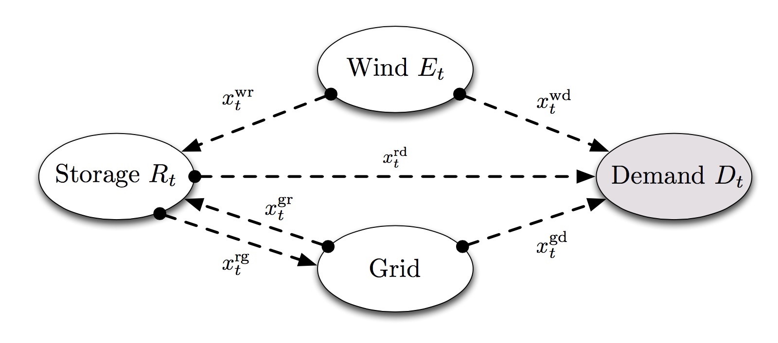
Figure 1: Energy system schematics

At the beginning of every period $t$ the manager must combine energy from different sources to satisfy the demand, $D_{t}$: energy currently in storage (represented by a decision $x_{t}^{rd}$); newly available wind energy (represented by a decision $x_{t}^{wd}$); energy from the grid (represented by a decision $x_{t}^{gd}$). Additionally, the manager must decide how much renewable energy to store, $x_{t}^{wr}$, how much energy, $x_{t}^{rg}$, to sell to the grid at price $P_{t}$, and how much energy to buy from the grid and store, $x_{t}^{gr}$. Hence, the manager’s decision variable at $t$ is defined as the vector $x_{t}=(x^{wd}_{t},x^{gd}_{t},x^{rd},x^{wr}_{t},x^{gr}_{t},x^{rg}_{t})^{T}\geq 0$, which should satisfy the following constraints:

$$x^{wd}_{t}+\beta^{d}x^{rd}_{t}+x^{gd}_{t} \leq D_{t},\qquad x^{wr}_{t}+x^{wd}_{t}\leq E_{t},\qquad x^{rd}_{t}+x^{rg}_{t}\leq R_{t},$$ (27)

$$x^{wr}_{t}+x^{gr}_{t}-x^{rd}_{t}-x^{rg}_{t} \leq R^{\max}-R_{t},\qquad x^{wr}_{t}+x^{gr}_{t}\leq\gamma^{c},\qquad x^{rd}_{t}+x^{rg}_{t}\leq\gamma^{d},$$ (28)

where $\gamma^{c}$ and $\gamma^{d}$ are the maximum amount of energy that can be charged or discharged from the storage device. Typically, $\gamma^{c}$ and $\gamma^{d}$ are the same.

The state variable at time $t$, $S_{t}$, includes the level of energy in storage, $R_{t}\in[0,R^{\max}]$ ($R^{\max}>0$ represents the storage capacity), the amount of energy available from wind and its forecast, $\{f^{E}_{t,t^{\prime}}\}_{t^{\prime}\geq t}(E_{t}=f^{E}_{t,t})$, the spot price of electricity from the grid and its forecast, $\{f^{P^{g}}_{t,t^{\prime}}\}_{t^{\prime}\geq t}(P^{g}_{t}=f^{P^{g}}_{t,t})$, the market price of electricity $P^{d}_{t}$, the demand $D_{t}$ and its forecast $\{f^{D}_{t,t^{\prime}}\}_{t^{\prime}\geq t}(D_{t}=f^{D}_{t,t})$, and the energy available from the grid $G_{t}$ at time $t$. Hence the state of the system can be represented by the vector $S_{t}=(R_{t},G_{t},f^{E}_{t,t^{\prime}},P^{m}_{t},f^{P^{g}}_{t,t^{\prime}},f^{D}_{t,t^{\prime}})\ \ \forall t^{\prime}\geq t$. In the Appendix, we describe how these forecasts can be generated.

The transition function, $S^{M}(\cdot)$ also explicitly describes the relationship between the state of the model at time $t$ and $t+1$ such that $S_{t+1}=S^{M}(S_{t},x_{t},W_{t+1})$, where $W_{t+1}=(E_{t+1},P_{t+1},D_{t+1})$ is the exogenous information revealed at $t+1$. In our numerical experiments, we assumed that $W_{t+1}$ is independent of $S_{t}$, but the CFA algorithm can work with any sample path provided by an exogenous source, which means it can handle an exogenous information process where $W_{t+1}$ may depend on $S_{t}$ and/or $x_{t}$. Indeed, the CFA method belongs to the class of data driven algorithms, where we do not need a model of the exogenous process. The relationship of storage levels between periods is defined as:

$$R_{t+1}=R_{t}-x^{rd}_{t}+\beta^{c}x^{wr}_{t}+\beta^{c}x^{gr}_{t}-x^{rg}_{t},$$ (29)

where $\beta^{c}\in(0,1)$ and $\beta^{d}\in(0,1)$, are the charge and discharge efficiencies. Denoting the penalty of not satisfying the demand by $C^{P}$, for given state $S_{t}$ and decision $x_{t}$, the profit realized at $t$ is given by

$$C_{t}(S_{t},x_{t})=C^{P}(D_{t}-x_{t}^{wd}-\beta^{d}x_{t}^{rd}-x_{t}^{gd})-P^{m}_{t}(x_{t}^{wd}+\beta^{d}x_{t}^{rd}+x_{t}^{gd})-P^{g}_{t}(\beta^{d}x^{rg}_{t}-x^{gr}_{t}-x^{gd}_{t}).$$ (30)

5.2 Policy Parameterizations

For our deterministic lookahead, by noting (30), we solve subproblem (4) subject to constraints (27) - (29) for $t^{\prime}\in[t+1,t+H]$. We call this deterministic lookahead policy the benchmark policy, and use it to estimate the degree to which the parameterized policies are able to improve the results in the presence of uncertainty. There are different ways of parameterizing the policy in this lookahead model. A few examples are as follows.

• Constant forecast parameterization - This parameterization uses a single scalar to modify the forecast amount of renewable energy for the entire horizon. Hence, the second constraint in (27) is changed to

  $$x^{wr}_{t,t^{\prime}}+x^{wd}_{t,t^{\prime}}\leq\theta\cdot f^{E}_{t,t^{\prime}}.$$ (31)

• Lookup table forecast parameterization - Overestimating or underestimating forecasts of renewable energy influences how aggressively a policy will store energy. We modify the forecast of renewable energy for each period of the lookahead model with a unique parameter $\theta_{\tau}$. This parameterization is a lookup table representation because there is a different $\theta$ for each lookahead period, $\tau=0,1,2,...$. This changes (31) to

  $$x^{wr}_{t,t^{\prime}}+x^{wd}_{t,t^{\prime}}\leq\theta_{t^{\prime}-t}\cdot f^{E}_{t,t^{\prime}}.$$ (32)

  where $t^{\prime}\in[t+1,t+H]$ and $\tau=t^{\prime}-t$. If $\theta_{\tau}<1$ the policy will be more conservative and decrease the risk of running out of energy. Conversely, if $\theta_{\tau}>1$ the policy will be more aggressive and less adamant about maintaining large energy reserves.

5.3 Numerical Experiments

In this subsection, we test the aforementioned parameterizations of the deterministic lookahead policy defined on variations of the energy storage problem by providing the same forecasts of exogenous information for the benchmark and parameterized policies. We say the parameterization $\theta$ outperforms the nonparametric benchmark policy if it has positive policy improvement $\Delta F^{\pi}(\theta)$, given by

$$\Delta F^{\pi}(\theta)=\frac{F^{\pi}(\theta)-F^{\text{D-LA}}}{|F^{\text{D-LA}}|},$$ (33)

where $F^{\pi}(\theta)$ is the average profit (negative cost defined in (30)) generated by $\theta$ and $F^{\text{D-LA}}$ is the average profit generated by the unparameterized deterministic lookahead policy described by equation (4). In all of our experiments, we compute these averaged profits over a testing data set including $1000$ random samples.

In our first set of experiments, we examine the performance of the lookup table parameterization policy with $H=23$ under perfect forecasts ($\sigma_{E}=0$) and noisy one ($\sigma^{2}_{E}=40$). In particular, we first set all values of $\theta$ to $1$ and then do a one-dimensional search over each coordinate of $\theta$. As it can be seen from Figure 2, under perfect forecasts, the optimal value for each coordinate of $\theta$ is $1$ while the others are set to $1$ as suggested by Lemma 4.4. However, when noisy forecasts are used, the optimal values for $\theta$ may be different than $1$.

Figure 2: Averaged performance of lookup parameterization policy under perfect forecasts (right) and noisy one ($\sigma^{2}_{E}=40$). Each curves represents performance of the lookup policy over changing one $\theta_{i}$ while $\theta_{j}=1\ \ \forall j\neq i$.

In the second set of experiments, we evaluate the performance of policies produced by our proposed stochastic approximation algorithms. In Algorithm 1, since the stochastic gradient given in (23) is not computable, we use numerical derivatives. Specifically, for each coordinate of the stochastic gradient, we use the finite-difference formula to estimate the corresponding partial derivatives by estimating the objective function at a given $\theta$ and its perturbations for each coordinate. We call this variant of Algorithm 1, the Stochastic Numerical Gradient method for the CFA model (SNG-CFA). Since our optimization problem is nonconvex, we implement our algorithms for several different starting points using $N=800$ iterations. We then evaluate the performance of the policy that is produced by averaging over a thousand simulations. We compare the performance of the optimized policies against the base policy using $\theta=1$ in Figures 3. We found that the RMSProp stepsize rule consistently outperformed AdaGrad, so RMSProp is used throughout. For the SGF-CFA method, we use a mini-batch of sample paths to compute stochastic gradients according to (15) and then use their average as an estimation for the gradient. To have a fair comparison, we use a mini-batch of size $12$ at each iteration of this algorithm so that its computational cost is similar to that of the SNG-CFA method. While the latter does not have theoretical finite-time convergence guarantees, we found that both algorithms have comparable practical performance.

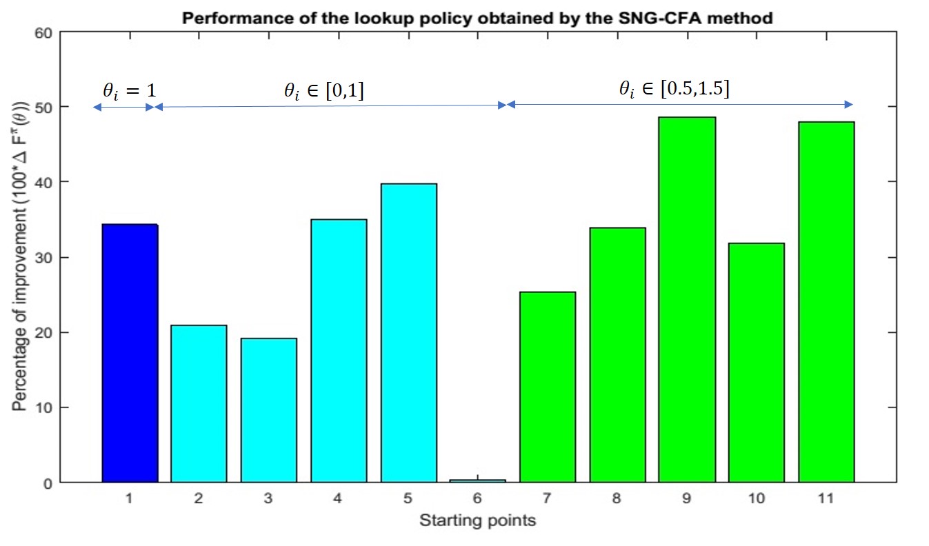
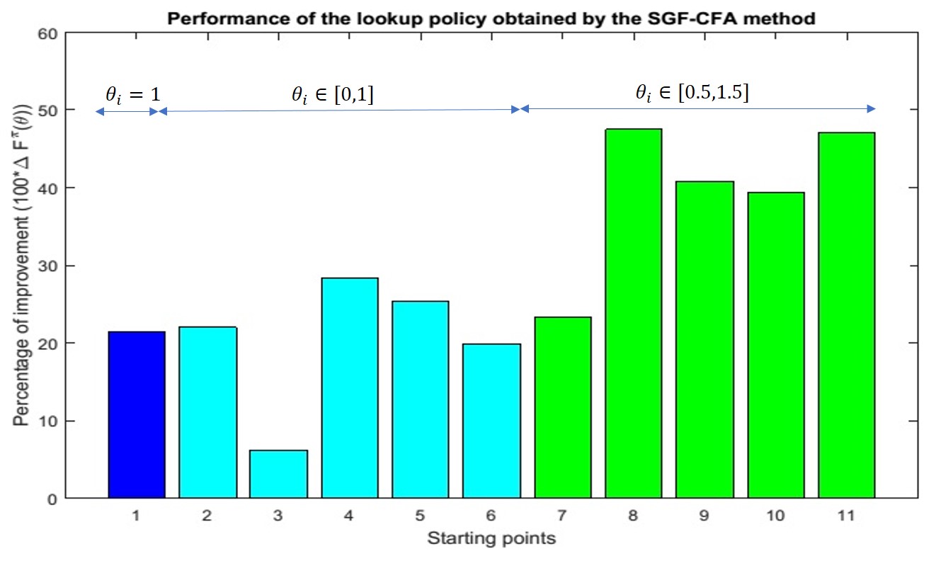
Figure 3: Left: Averaged performance of the output policy of the SNF-CFA method (left) and the SGF-CFA method with batch size of $12$ (right), using RMSProp stepsize for $\sigma^{2}_{E}=40$ over $1000$ simulations with different starting points.

In the next set of experiments, we explored the structure of the response surface in our optimization problem by doing a two-dimensional grid search for different pairs of coordinates of $\theta$ in the lookup table representation form, while keeping the other coordinates unchanged. We show the improvement in the objective function over the benchmark policy ($\theta=1$) in Figure 4 (more are shown in Appendix II). All graphs contain ridges on which changing the coordinates does not improve the policy. While the shape of the ridges can be quite different from one pair of coordinates to another one, most of them share some kind of unimodularity.

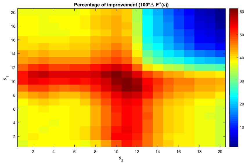
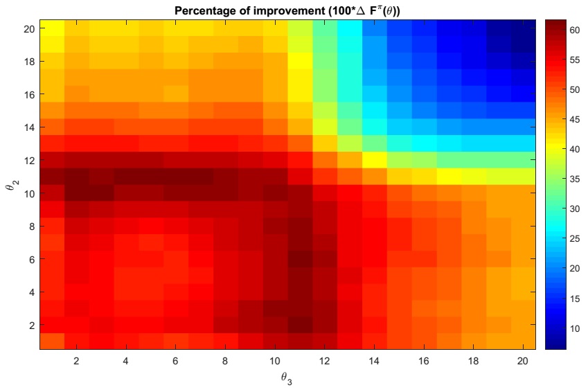
Figure 4: Averaged performance of lookup policies under noisy forecast. Each graph represents improvements over a two-dimensional grid surface of pairs of coordinates of $\theta$.

6 Conclusion

This work builds upon a long history of using deterministic optimization models to solve sequential stochastic problems. Unlike other deterministic methods, our class of methods, CFAs, parametrically modify deterministic approximations to account for problem uncertainty. Our particular use of modified linear programs within the framework of the CFA represents a fundamentally new approach for solving multistage stochastic programming problems. Our method allows us to exploit the structural properties of the problem while capturing the complex dynamics of the full base model, rather than accepting the approximations required in a stochastic lookahead model.

The parametric CFA approach indeed represents an alternative to stochastic lookahead models that represent the foundation of stochastic programming. It requires some intuition into how uncertainty might affect the optimal solution. We would argue that this requirement parallels the design of any parametric statistical model, and hence enjoys a long history. We believe there are many problems where practitioners have a good sense of how uncertainty affects the solution. This approach opens up entirely new lines of research.

Acknowledgments

This research has been supported in part by the National Science Foundation, grant CMMI-1537427.

Appendix I

$1$. Renewable energy and demand model

Our model is designed in part to create complex nonstationary behaviors to test the ability of our policy to exploit forecasts while managing uncertainty. We use a series of recursive equations to create a realistic model of the stochastic process describing the generation of renewable energy. In particular, letting $f^{E}_{t,t^{\prime}}$ be the forecast of the renewable energy at time $t$ for time $t^{\prime}$ and assuming that $\{f^{E}_{0,t^{\prime}}\}_{t^{\prime}=0,\ldots,\min(H,T)}$ is given, we define

$$f^{E}_{t+1,t^{\prime}}=f^{E}_{t,t^{\prime}}+\epsilon_{t+1,t^{\prime}}\qquad t=0,\ldots,T-1,\qquad t^{\prime}=t+1,\ldots,\min(t+H,T)$$ (34)

where $\epsilon_{t+1,t^{\prime}}$ represents the level of noise whose distribution depends on $f^{E}_{t,t^{\prime}}$. To create such noise, we first construct a symmetric matrix $\Sigma\in\mathbb{R}^{H\times H}$ such that $\Sigma(i,j)=\sigma_{E}^{2}e^{-\alpha|i-j|}\ \ \forall i,j$, where $\sigma_{E},\alpha>0$ are constant numbers. Indeed, we can manipulate the quality of the forecast by changing $\sigma_{E}$. By construction, $\Sigma$ acts as a covariance matrix representing less correlation between the $i$-th and $j$-th elements when they are far from each other. We then define a normal noise vector as

$$\bar{\epsilon}_{t}=L\cdot Z_{t},$$

where $L$ is the lower triangular Cholesky decomposition of $\Sigma$ and $Z_{t}\sim{\cal N}(0,I_{H\times H})$. Hence, each element of $\bar{\epsilon}_{t}$ has a normal distribution with zero mean and variance $\sigma_{E}^{2}$ due to the fact that $\Sigma=L\cdot L^{\top}$ and $\Sigma(i,i)=1$. However, these elements are correlated by construction. To avoid nonnegativity of the forecast, we set

$$[\epsilon_{t+1,t+1},\ldots,\epsilon_{t+1,\min(t+H,T)}]^{\top}=F_{EM}^{-1}(\phi(trc^{t}_{H}(\bar{\epsilon}_{t}))),$$

where the operator $trc^{t}_{H}(y)$ truncates the first $\min(H,T-t)$ elements of vector $y$, $\phi(\cdot)$ is standard normal density function, and $F_{EM}$ is an empirical cumulative distribution function obtained from historical data. The choice of $F_{EM}$ depends on ${f^{E}}_{t,t^{\prime}}$ for $t^{\prime}=t+1,\ldots,\min(t+H,T)$. Figure 5 shows five examples of empirical cumulative distribution functions for the change in wind speed, used in our experiments. It should be mentioned that if ${f^{E}}_{t,t^{\prime}}$ becomes negative (by low chance), we just map it to $0$. Finally, after generating all forecasts, we force the observed value of the renewable energy at time $t$ to be ${f^{E}}_{t,t}$.

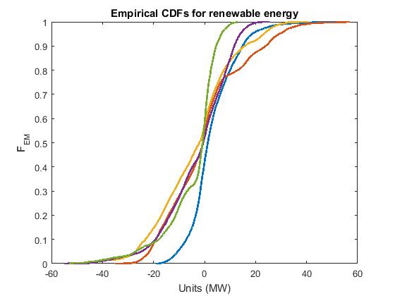
Figure 5: Empirical cumulative distribution functions from a real data set for the renewable energy.

A generated sample of observed renewable energy and its prospective forecast can be viewed in Figure 6. This is an example of a complex stochastic process that causes problems for stochastic lookahead models. For example, it is very common when using the stochastic dual dynamic programming (SDDP) to assume interstage independence, which means that $W_{t}$ and $W_{t+1}$ are independent, which is simply not the case in practice (Shapiro et al. (2013) and Dupačová and Sladkỳ (2002)). However, capturing this dynamic in a stochastic lookahead model is quite difficult. Our CFA methodology, however, can easily handle these more complex stochastic models since we only need to be able to simulate the process in the base model.

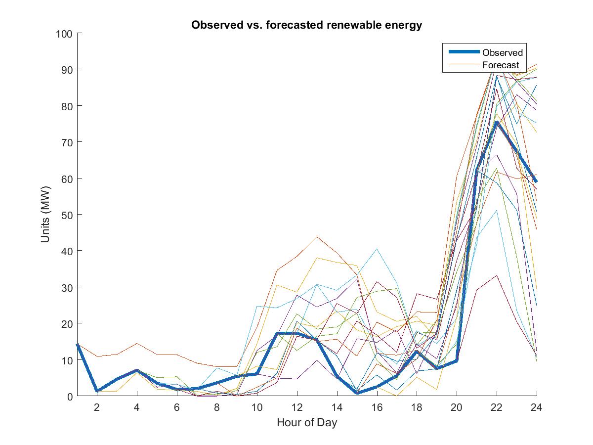
Figure 6: Generated sample of renewable energy ($E_{t}$)

We use the above approach in a backward format to generate demand forecasts. More specifically, assuming that $\{f^{D}_{t,t}\}_{t=0,\ldots,T}$ is given, we define

$$f^{D}_{t-1,t^{\prime}}=f^{D}_{t,t^{\prime}}+trc^{t-1}_{H}(\bar{\epsilon}_{t-1,t^{\prime}})\qquad t=T,\ldots,1,\qquad t^{\prime}=t,\ldots,\min(t+H,T).$$ (35)

Note that since the observed demands are set in advance, we can avoid the nonnegativity issue without using the aforementioned inverse CDF of a (uniform) random variable. Indeed, since the observed demands are usually cyclic, their values are specified with a sinusoidal stochastic function:

$$f^{D}_{t,t}=D_{t}=\lceil\max\{0,D-\hat{D}\sin\bigg{(}\frac{\bar{D}\pi t}{T}\bigg{)}+e_{t}\}\rceil\qquad t=0,1,\ldots,T,$$ (36)

where $\{e_{t}\}_{t\geq 0}$ are correlated standard normal random variables and $D>\hat{D},\bar{D}$ are positive constants. A generated sample of observed demand and its prospective forecast can be viewed in Figure 7.

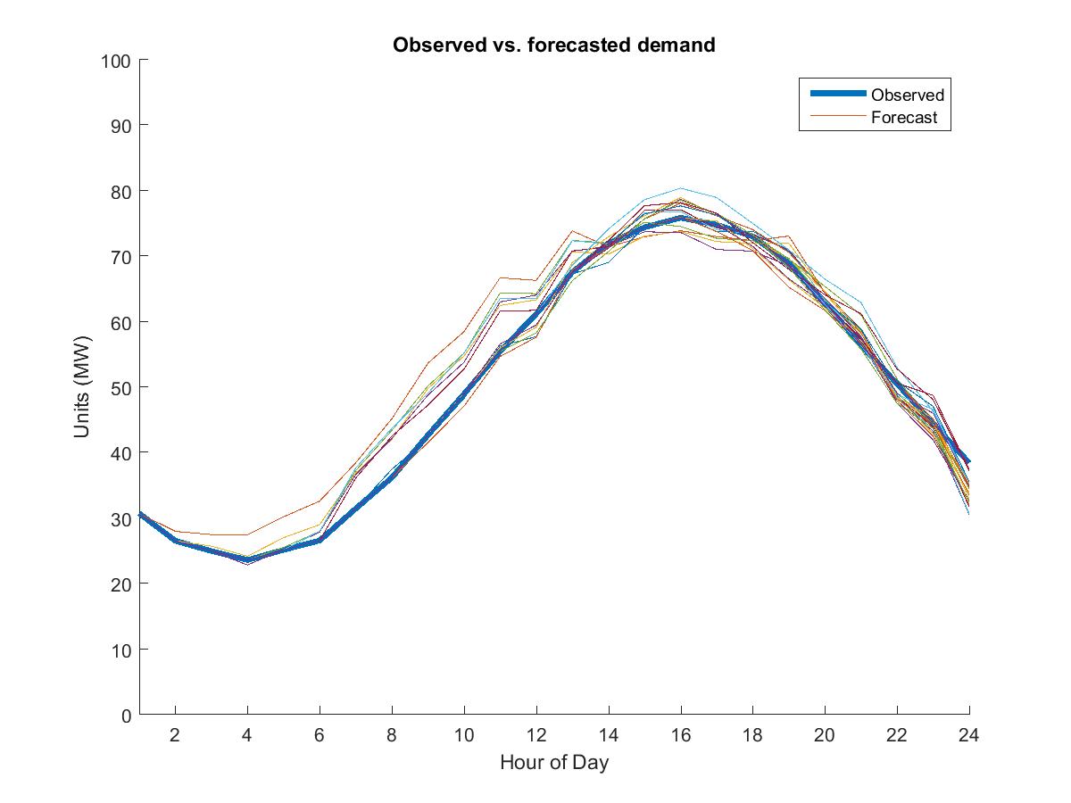
Figure 7: Generated sample of demand ($D_{t}$)

$2$. Spot price model

We assume that spot price of electricity from the grid has a positive correlation with the demand. In particular, we set

$$f^{P}_{t,t^{\prime}}=a+bf^{D}_{t,t^{\prime}}\qquad t=0,1,\ldots,T,\qquad t^{\prime}=t,t+1,\ldots,T,$$

where $b>0$ and $a\sim{\cal N}(\mu_{p},\sigma_{p})$ for some $\mu_{p},\sigma_{p}\geq 0$. Moreover, the observed and forecasted market prices are fixed and set to the average of all forecasted grid prices assuming a long-term contract with the customer.

Appendix II

Extended Numerical Experiments

In this Section, we provide more numerical experiments about the energy storage problem described in Section 5. In the first one, we evaluate the performance of the constant forecast parameterization for different levels of uncertainty in forecasting the supply from renewable energy. In this case, the optimization problem is one dimensional and hence, we use a grid search to find the optimal policy. As shown in Figure 8, performance of the constant parameterization policy is improved by increasing the value of $\theta$ to one point and then decreased. It is also worth noting that under perfect forecasts, $\theta=1$ is the optimal value as mentioned before.

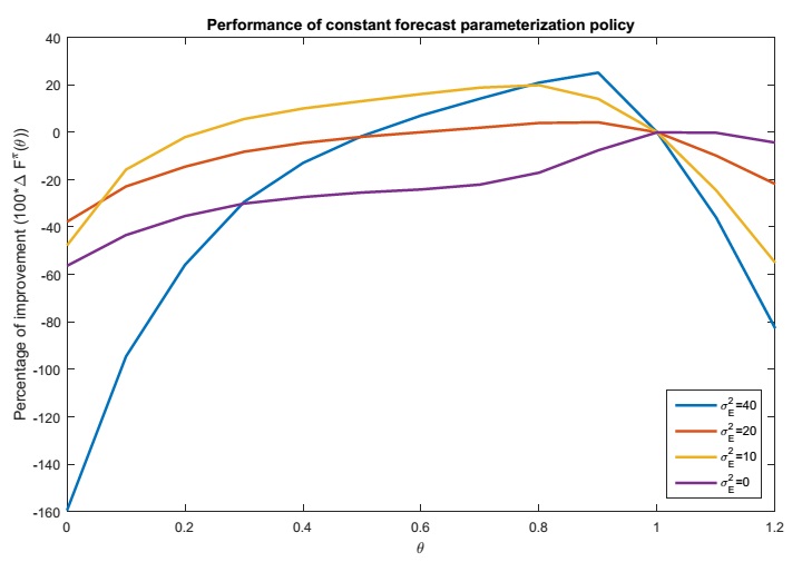
Figure 8: Averaged performance of constant parameterization policy over $1000$ simulation.

In the next set of experiments, we provide more graphs in Figure 4 about the behaviour of the objective function in terms of improvement over the benchmark policy for different pairs of coordinates of $\theta$ in the lookup up table representation form.

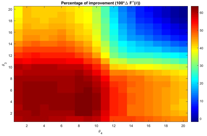
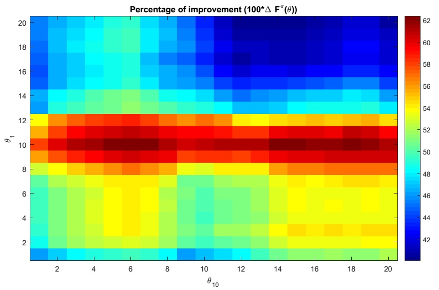
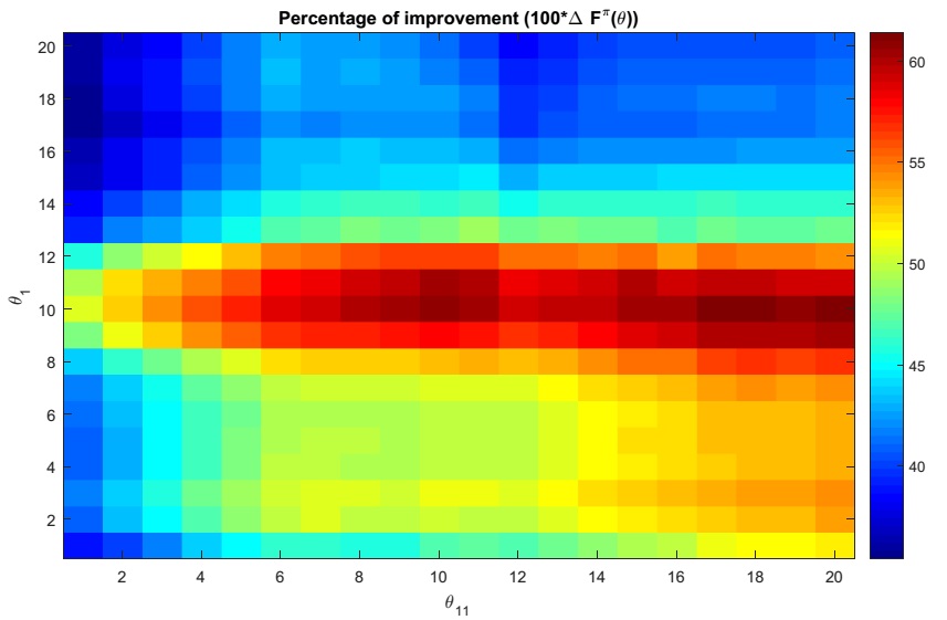
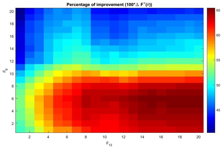
Figure 9: Averaged performance of lookup policies under noisy forecast. Each graph represents improvements over a two-dimensional grid surface of pairs of coordinates of $\theta$.

References

- (1)
- Bertsekas (2011) Bertsekas, D. P. (2011), ‘Dynamic programming and optimal control 3rd edition’, Vol. II, Belmont, MA: Athena Scientific .
- Bertsimas and Goyal (2012) Bertsimas, D. and Goyal, V. (2012), ‘On the power and limitations of affine policies in two-stage adaptive optimization’, Mathematical programming 134(2), 491–531.
- Bertsimas et al. (2011) Bertsimas, D., Iancu, D. A. and Parrilo, P. A. (2011), ‘A hierarchy of near-optimal policies for multistage adaptive optimization’, IEEE Transactions on Automatic Control 56(12), 2809–2824.
- Birge and Louveaux (2011) Birge, J. R. and Louveaux, F. (2011), Introduction to stochastic programming, Springer Science & Business Media.
- Camacho and Alba (2013) Camacho, E. F. and Alba, C. B. (2013), Model predictive control, Springer Science & Business Media.
- Cao (2008) Cao, X.-R. (2008), ‘Stochastic learning and optimization-a sensitivity-based approach’, IFAC Proceedings Volumes 41(2), 3480–3492.
- Carpentier et al. (2015) Carpentier, P.-L., Gendreau, M. and Bastin, F. (2015), ‘Managing hydroelectric reservoirs over an extended horizon using benders decomposition with a memory loss assumption’, IEEE Transactions on Power Systems 30(2), 563–572.
- Chau et al. (2014) Chau, M., Fu, M. C., Qu, H. and Ryzhov, I. O. (2014), Simulation optimization: a tutorial overview and recent developments in gradient-based methods, in ‘Proceedings of the 2014 Winter Simulation Conference’, IEEE Press, pp. 21–35.
- Deisenroth et al. (2013) Deisenroth, M. P., Neumann, G. and Peters, J. (2013), ‘A survey on policy search for robotics’, Foundations and Trends in Robotics 2(1-2), 1–142.
- Donohue and Birge (2006) Donohue, C. J. and Birge, J. R. (2006), ‘The abridged nested decomposition method for multistage stochastic linear programs with relatively complete recourse’, Algorithmic Operations Research 1(1).
- Duchi et al. (2011) Duchi, J., Hazan, E. and Singer, Y. (2011), ‘Adaptive subgradient methods for online learning and stochastic optimization’, Journal of Machine Learning Research 12, 2121–2159.
- Dupačová and Sladkỳ (2002) Dupačová, J. and Sladkỳ, K. (2002), ‘Comparison of multistage stochastic programs with recourse and stochastic dynamic programs with discrete time’, ZAMM-Journal of Applied Mathematics and Mechanics/Zeitschrift für Angewandte Mathematik und Mechanik 82(11-12), 753–765.
- Fu (2015) Fu, M. C., ed. (2015), Handbook of simulation optimization, Springer.
- Ghadimi and Lan (2013) Ghadimi, S. and Lan, G. (2013), ‘Stochastic first- and zeroth-order methods for nonconvex stochastic programming’, SIAM Journal on Optimization 23(4), 2341–2368.
- Glasserman (1991) Glasserman, P. (1991), Gradient estimation via perturbation analysis, Vol. 116, Springer Science & Business Media.
- Hadjiyiannis et al. (2011) Hadjiyiannis, M. J., Goulart, P. J. and Kuhn, D. (2011), ‘An efficient method to estimate the suboptimality of affine controllers’, IEEE Transactions on Automatic Control 56(12), 2841–2853.
- Han and E (2016) Han, J. and E, W. (2016), ‘Deep learning approximation for stochastic control problems’, arXiv preprint arXive:1611.07422 .
- Harrison and Van Mieghem (1999) Harrison, J. M. and Van Mieghem, J. A. (1999), ‘Multi-resource investment strategies: Operational hedging under demand uncertainty’, European Journal of Operational Research 113(1), 17–29.
- Ho (1992) Ho, Y.-C. (1992), Discrete event dynamic systems: analyzing complexity and performance in the modern world, IEEEPress, New York.
- Hu et al. (2007) Hu, J., Fu, M. C., Ramezani, V. R. and Marcus, S. I. (2007), ‘An evolutionary random policy search algorithm for solving markov decision processes’, INFORMS Journal on Computing 19(2), 161–174.
- Jin et al. (2011) Jin, S., Ryan, S. M., Watson, J.-P. and Woodruff, D. L. (2011), ‘Modeling and solving a large-scale generation expansion planning problem under uncertainty’, Energy Systems 2(3-4), 209–242.
- Kushner and Yin (2003) Kushner, H. J. and Yin, G. (2003), Stochastic approximation and recursive algorithms and applications, Vol. 35, Springer Science & Business Media.
- Lan et al. (2006) Lan, S., Clarke, J.-P. and Barnhart, C. (2006), ‘Planning for robust airline operations: Optimizing aircraft routings and flight departure times to minimize passenger disruptions’, Transportation science 40(1), 15–28.
- Levine and Abbeel (2014) Levine, S. and Abbeel, P. (2014), Learning neural network policies with guided policy search under unknown dynamics, in ‘Advances in Neural Information Processing Systems’, pp. 1071–1079.
- Lillicrap et al. (2015) Lillicrap, T. P., Hunt, J. J., Pritzel, A., Heess, N., Erez, T., Tassa, Y., Silver, D. and Wierstra, D. (2015), ‘Continuous control with deep reinforcement learning’, arXiv preprint arXiv:1509.02971 .
- Lium et al. (2009) Lium, A.-G., Crainic, T. G. and Wallace, S. W. (2009), ‘A study of demand stochasticity in service network design’, Transportation Science 43(2), 144–157.
- Mannor et al. (2003) Mannor, S., Rubinstein, R. Y. and Gat, Y. (2003), The cross entropy method for fast policy search, in ‘ICML’, pp. 512–519.
- Mulvey et al. (1995) Mulvey, J. M., Vanderbei, R. J. and Zenios, S. A. (1995), ‘Robust optimization of large-scale systems’, Operations research 43(2), 264–281.
- Nesterov and Spokoiny (2017) Nesterov, Y. and Spokoiny, V. (2017), ‘Random gradient-free minimization of convex functions’, Foundations of Computational Mathematics 17(2), 527–566.
- Ng and Jordan (2000) Ng, A. Y. and Jordan, M. (2000), Pegasus: A policy search method for large mdps and pomdps, in ‘Proceedings of the Sixteenth conference on Uncertainty in artificial intelligence’, Morgan Kaufmann Publishers Inc., pp. 406–415.
- Peshkin et al. (2000) Peshkin, L., Kim, K.-E., Meuleau, N. and Kaelbling, L. P. (2000), Learning to cooperate via policy search, in ‘Proceedings of the Sixteenth conference on Uncertainty in artificial intelligence’, Morgan Kaufmann Publishers Inc., pp. 489–496.
- Powell (2011) Powell, W. B. (2011), Approximate Dynamic Programming: Solving the Curses of Dimensionality, Wiley.
- Powell et al. (2004) Powell, W., Ruszczyński, A. and Topaloglu, H. (2004), ‘Learning algorithms for separable approximations of discrete stochastic optimization problems’, Mathematics of Operations Research 29(4), 814–836.
- Robbins and Monro (1951) Robbins, H. and Monro, S. (1951), ‘A stochastic approximation method’, The annals of mathematical statistics pp. 400–407.
- Sethi and Sorger (1991) Sethi, S. and Sorger, G. (1991), ‘A theory of rolling horizon decision making’, Annals of Operations Research 29(1), 387–415.
- Shapiro et al. (2013) Shapiro, A., Tekaya, W., da Costa, J. P. and Soares, M. P. (2013), ‘Risk neutral and risk averse stochastic dual dynamic programming method’, European journal of operational research 224(2), 375–391.
- Strassen (1965) Strassen, V. (1965), ‘The existence of probability measures with given marginals’, Annals of Mathematical Statistics 38, 423–439.
- Sutton and Barto (2018) Sutton, R. S. and Barto, A. G. (2018), Reinforcement learning: An introduction, Second Edition, MIT press, Cambridge.
- Sutton et al. (1999) Sutton, R. S., McAllester, D. A., Singh, S. P., Mansour, Y. et al. (1999), Policy gradient methods for reinforcement learning with function approximation., in ‘NIPS’, Vol. 99, Citeseer, pp. 1057–1063.
- Tieleman and Hinton (2012) Tieleman, T. and Hinton, G. (2012), Lecture 6.5-rmsprop: Divide the gradient by a running average of its recent magnitude, in ‘COURSERA: Neural Networks for Machine Learning’.
- Wallace and Fleten (2003) Wallace, S. W. and Fleten, S.-E. (2003), ‘Stochastic programming models in energy’, Handbooks in operations research and management science 10, 637–677.