A note on $2\times 2$ block-diagonal preconditioning

Abstract

For $2\times 2$ block matrices, it is well-known that block-triangular or block-LDU preconditioners with an exact Schur complement (inverse) converge in at most two iterations for fixed-point or minimal-residual methods. Similarly, for saddle-point matrices with a zero (2,2)-block, block-diagonal preconditioners converge in at most three iterations for minimal-residual methods, although they may diverge for fixed-point iterations. But, what happens for non-saddle-point matrices and block-diagonal preconditioners with an exact Schur complement? This note proves that minimal-residual methods applied to general $2\times 2$ block matrices, preconditioned with a block-diagonal preconditioner, including an exact Schur complement, do not (necessarily) converge in a fixed number of iterations. Furthermore, examples are constructed where (i) block-diagonal preconditioning with an exact Schur complement converges no faster than block-diagonal preconditioning using diagonal blocks of the matrix, and (ii) block-diagonal preconditioning with an approximate Schur complement converges as fast as the corresponding block-triangular preconditioning. The paper concludes by discussing some practical applications in neutral-particle transport, introducing one algorithm where block-triangular or block-LDU preconditioning are superior to block-diagonal, and a second algorithm where block-diagonal preconditioning is superior both in speed and simplicity.

65F08

1 $2\times 2$ block preconditioners

Consider a block $2\times 2$ matrix equation,

(1) $$\begin{bmatrix}A_{11}&A_{12}\\ A_{21}&A_{22}\end{bmatrix}\begin{bmatrix}\mathbf{x}_{1}\\ \mathbf{x}_{2}\end{bmatrix}\begin{bmatrix}\mathbf{b}_{1}\\ \mathbf{b}_{2}\end{bmatrix},$$

where $A_{11}$ and $A_{22}$ are square (although potentially different sizes), and at least one is invertible. Here we assume without loss of generality that $A_{11}$ is nonsingular, and focus on the case of $A_{22}\neq\mathbf{0}$ (we refer to the case of $A_{22}=\mathbf{0}$ as saddle-point in this paper, unless otherwise specified).

Such systems arise in numerous applications, and are often solved iteratively using either fixed-point or Krylov methods with some form of block preconditioning [3, 22]. The four most common block preconditioners are block diagonal, block upper triangular, block lower triangular, and block LDU, which we will denote $D$, $U$, $L$, and $M$, respectively. It is generally believed that one of the diagonal blocks in these preconditioners must approximate the appropriate Schur complement. Given we assumed $A_{11}$ to be nonsingular, here we focus on the $(2,2)$-Schur complement, ${S}_{22}:=A_{22}-A_{21}A_{11}^{-1}A_{12}$. Assume the action of ${S}_{22}^{-1}$ and $A_{11}^{-1}$ are available, and define block preconditioners as follows:

$$L :=\begin{bmatrix}{A}_{11}&\mathbf{0}\\ A_{21}&{S}_{22}\end{bmatrix},\hskip 27.55544ptU:=\begin{bmatrix}{A}_{11}&A_{12}\\ \mathbf{0}&{S}_{22}\end{bmatrix},$$

(2) $$D_{\pm} :=\begin{bmatrix}{A}_{11}&\mathbf{0}\\ \mathbf{0}&\pm{S}_{22}\end{bmatrix},\hskip 12.91663pt\widehat{D}_{\pm}:=\begin{bmatrix}{A}_{11}&\mathbf{0}\\ \mathbf{0}&\pm{A}_{22}\end{bmatrix},$$

$$M :=\begin{bmatrix}I&\mathbf{0}\\ A_{21}A_{11}^{-1}&I\end{bmatrix}\begin{bmatrix}A_{11}&\mathbf{0}\\ \mathbf{0}&{S}_{22}\end{bmatrix}\begin{bmatrix}I&A_{11}^{-1}A_{12}\\ \mathbf{0}&I\end{bmatrix}.$$

Note, $\widehat{D}$ is a (more practical) variation on block-diagonal preconditioning that assumes $A_{22}$ is nonsingular and its inverse available, rather than the Schur complement ${S}_{22}$. The $\pm$ subscript on block-diagonal preconditioners corresponds to the sign on the (2,2)-block. For the common case of a symmetric indefinite matrix $A$, with $A_{22}$ symmetric negative definite (SND) and $A_{11}$ symmetric positive definite (SPD), block-diagonal preconditioners with a negative (2,2)-block (like $D_{-}^{-1}$ or $\widehat{D}_{-}^{-1}$) are SPD, and a three-term recursion such as preconditioned MINRES can be applied [15].

In the following, we restate and tighten known results regarding fixed-point and minimal residual iterations [15, 17] in exact arithmetic, using preconditioners in (1), for the general case (1) and the saddle-point case, where $A_{22}=\mathbf{0}$. First, note the following proposition.

Proposition 1.1.

Let $A_{11}$ be invertible. Then dim(ker($A))=$ dim(ker($S_{22}$)).

Proof 1.2.

Note that if $A$ is singular, $\exists$ $\mathbf{s}$ such that $A\mathbf{s}=\mathbf{0}$. Under the assumption that $A_{11}$ is nonsingular, expanding $A\mathbf{s}$ in $2\times 2$ block form (1) shows that $A$ can be singular if and only if ${S}_{22}\mathbf{s}_{2}=\mathbf{0}$, with corresponding ker$(A)=[-A_{11}^{-1}A_{12}\mathbf{s}_{2};\mathbf{s}_{2}]$. Thus the dimension of ker$(A)$ equals the dimension of ker$(S_{22})$, and $A$ is nonsingular if and only if $S_{22}$ is nonsingular.

For block-diagonal preconditioner $D_{\pm}$, there is an implicit assumption that $A_{11}$ and $S_{22}$ are invertible, in which case (by Proposition 1.1) $A$ is invertible and $D_{\pm}^{-1}A$ is invertible. Proofs regarding the number of preconditioned minimal-residual iterations to exact convergence with preconditioner $D_{\pm}$ in [11, 10] include the possibility of a zero eigenvalue in the characteristic polynomial. Since this cannot be the case, the maximum number of iterations is three, not four as originally stated in [11, 10] (see Proposition 1.4).

Proposition 1.3 ($2\times 2$ block preconditioners).

1. Fixed-point iterations [20] and minimal residual methods [11, 10] preconditioned with $L$, $U$, and $M$ converge in at most two iterations.

2. If $A_{11}$ and $A_{22}$ are nonsingular, convergence of fixed-point and minimal residual methods preconditioned with $\widehat{D}_{\pm}$ is defined by convergence of an equivalent method applied to the preconditioned Schur complements, $\pm A_{11}^{-1}{S}_{11}$ and $\pm A_{22}^{-1}{S}_{22}$ (roughly twice the number of iterations as the larger of the two) [20].

Proposition 1.4 ($2\times 2$ block saddle-point preconditioners ($A_{22}=\mathbf{0})$).

1. Fixed-point iterations preconditioned with $D_{\pm}$ do not necessarily converge [20].

2. Minimal residual methods preconditioned with $D_{\pm}$ converge in at most three iterations (see [11, 10], and Proposition 1.1).

Note that block-triangular and LDU-type preconditioners have a certain optimality – in exact arithmetic and using the exact Schur complement, convergence is guaranteed in two iterations, while convergence using an approximate Schur complement is exactly defined by the preconditioned Schur complement-problem. This provides general guidance in the development of block preconditioners, that the Schur complement should be well approximated for a robust method.

The above propositions suggest one might also want a block-diagonal preconditioner to approximate the Schur complement in one of the blocks. Indeed, block-diagonal preconditioners are often designed to approximate a Schur complement in one of the blocks (for example, see [18]). However, it turns out that block-diagonal preconditioners with an exact Schur complement, for $A_{22}\neq\mathbf{0}$, are not optimal in the sense that block-triangular and LDU preconditioners are. That is, block-diagonally preconditioned minimal-residual methods are not guaranteed to converge in $\mathcal{O}(1)$ iterations (see Section 2 and Theorem 2.1), and convergence is not defined by the preconditioned Schur complement.

Numerous papers have looked at eigenvalue analyses for block preconditioning (for example, [4, 7, 2, 5, 11, 10, 1, 18, 12, 16]). This paper falls into the series of notes on the spectrum of various block preconditioners with exact inverses [11, 10, 4, 5], here presenting results for the nonsymmetric and non-saddle-point, block-diagonal case. In addition to the notes, this work is perhaps most related to [18]. There, a lengthy eigenvalue analysis is done on approximate block-diagonal preconditioning, with approximations to $A_{11}^{-1}$ and $S_{22}^{-1}$, but the cases of exact inverses as in (1) are not directly considered or discussed.

Section 2 presents the new theory, deriving the spectrum of preconditioned operators $D_{\pm}^{-1}A$ and $\widehat{D}_{\pm}^{-1}A$ as a nonlinear function of the rank of $A_{12}$ and $A_{21}$, and the generalized eigenvalues of matrix pencils $(A_{22},S_{22})$ or $(S_{22},A_{22})$. A brief discussion on implications, particularly for symmetric matrices is given in Section 2.1, where examples are constructed to show that block-diagonal preconditioning with an exact Schur compelment can converge relatively slowly, that block-diagonal preconditioning with an approximate Schur complement can be as fast as, or significantly slower than, block triangular preconditioning (rather than $\approx 2\times$ slower when $A_{22}=\mathbf{0}$ [8]), and that block-diagonal preconditioning is likely more robust with symmetric indefinite matrices than SPD. A practical example in the simulation of neutral-particle transport is discussed in Section 3.

2 Block-diagonal preconditioning

It is shown in [11, 10] that block-diagonal and block-triangular preconditioners for saddle-point problems, with an exact Schur complement, have three and two nonzero eigenvalues. Thus, the minimal polynomial for minimal residual methods will be exact in a Krylov space of at most that size.

Theorem 2.1 derives the full eigenvalue decomposition for general $2\times 2$ operators, preconditioned by the block-diagonal preconditioners $D_{\pm}^{-1}$ and $\widehat{D}_{\pm}^{-1}$. In particular, the spectrum of the preconditioned operator is fully defined by the generalized eigenvalue problems $A_{22}\mathbf{y}=\widetilde{\lambda}S_{22}\mathbf{y}$ or $S_{22}\mathbf{y}=\widehat{\lambda}A_{22}\mathbf{y}$, depending on whether we assume $S_{22}$ or $A_{22}$ are nonsingular, respectively. If $A_{22}=\mathbf{0}$, then $\widetilde{\lambda}=0$, and the results from [11, 10] immediately follow. For $A_{22}\neq\mathbf{0}$, the preconditioned operator can have more eigenvalues, up to a full set of $n$ distinct eigenvalues (or, the generalized eigenvectors could not form a complete basis for the space), and no such statements can be made on the guaranteed convergence of minimal-residual methods.

Theorem 2.1 (Eigendecomposition of block-diagonal preconditioned operators).

Assume that $A_{11}$ and $S_{22}$ are invertible. Let $\{\widetilde{\lambda},\mathbf{v}_{2}\}$ be a generalized eigenpair of $A_{22}\mathbf{v}_{2}=\widetilde{\lambda}S_{22}\mathbf{v}_{2}$. Then, the spectra of the preconditioned operator for block-diagonal preconditioners $D_{\pm}^{-1}$ (1) are given by:

$$\sigma(D_{+}^{-1}A) =\left(\frac{\widetilde{\lambda}+1}{2}\pm\frac{1}{2}\sqrt{(\widetilde{\lambda}-1)(\widetilde{\lambda}+3)}\right)\quad\mathbin{\scalebox{1.5}{$\cup$}}\quad\left\{1\right\},$$

$$\sigma({D}_{-}^{-1}A) =\left(-\frac{\widetilde{\lambda}-1}{2}\pm\frac{1}{2}\sqrt{(\widetilde{\lambda}-1)^{2}+4}\right)\quad\mathbin{\scalebox{1.5}{$\cup$}}\quad\left\{\pm 1\right\}.$$

Assume that $A_{11}$ and $A_{22}$ are invertible. Now let $\{\widehat{\lambda},\mathbf{v}_{2}\}$ be a generalized eigenpair of $S_{22}\mathbf{v}_{2}=\widehat{\lambda}A_{22}\mathbf{v}_{2}$. Then, the spectra of the preconditioned operator for block-diagonal preconditioners $\widehat{D}_{\pm}^{-1}$ (1) are given by:

$$\sigma(\widehat{D}_{+}^{-1}A) =\left(1\pm\sqrt{1-\widehat{\lambda}}\right)\quad\mathbin{\scalebox{1.5}{$\cup$}}\quad\left\{\pm 1\right\},$$

$$\sigma(\widehat{D}_{-}^{-1}A) =\left(\pm\sqrt{\widehat{\lambda}}\right)\quad\mathbin{\scalebox{1.5}{$\cup$}}\quad\left\{\pm 1\right\}.$$

The multiplicity of the $\{\pm 1\}$ eigenvalues are given by the dimensions of the nullspace of $A_{12}$ and $A_{21}$. Eigenvectors for each eigenvalue can also be written in a closed form as a function of $\mathbf{v}_{2}$, and are derived in the proof (see Section 2.2).

Now assume $A_{12}A_{22}^{-1}A_{21}$ is nonsingular. By continuity of eigenvalues as a function of matrix entries,

$$\lim_{A_{22}\to 0}\sigma(D_{+}^{-1}A) =\left\{1,\frac{1\pm\mathrm{i}\sqrt{3}}{2}\right\},\hskip 21.52771pt\lim_{A_{22}\to 0}\sigma(D_{-}^{-1}A)=\left\{1,\frac{1\pm\sqrt{5}}{2}\right\},$$

and the maximum number of iterations for exact convergence of minimal-residual methods converges to three. Note that the limit of $\sigma(D_{-}^{-1}A)$ does not include $-1$ because by assuming $A_{12}A_{22}^{-1}A_{21}$ is nonsingular, there is an implicit assumption that ket$(A_{12})=\emptyset$, which means $\not\exists$ an eigenvalue of $-1$ (see Lemma 2.6).

2.1 Discussion

The primary implication of Theorem 2.1 is that block-diagonal preconditioned minimal-residual methods with an exact Schur complement do not necessarily converge in a fixed number of iterations. Recall block-diagonal preconditioning is often applied to symmetric matrices for use with MINRES, and convergence of such Krylov methods is better understood than GMRES, Here, we include a brief discussion on the eigenvalues of block-diagonally preconditioned symmetric $2\times 2$ block matrices with semi-definite diagonal blocks.

Consider real-valued, symmetric, nonsingular matrices with nonzero saddle-point structure, that is,

(3) $$A=\begin{bmatrix}A_{11}&A_{12}\\ A_{12}^{T}&A_{22}\end{bmatrix},$$

where $A_{11}$ is SPD and $A_{22}\neq\mathbf{0}$ is symmetric semidefinite (positive or negative definite). Such matrices arise often in practice; see review papers [3, 22] for many different examples. From Theorem 2.1, we can consider the spectrum of the preconditioned operator based on the generalized spectrum of $(S_{22},A_{22})$. Figure 1 plots the magnitude of eigenvalues $\lambda\in\sigma(D_{\pm}^{-1}A)$ and $\lambda\in\sigma(\widehat{D}_{\pm}^{-1}A)$ as a function of $\widetilde{\lambda}$ in a log-log scale (excluding zero on the logarithmic x-axis).

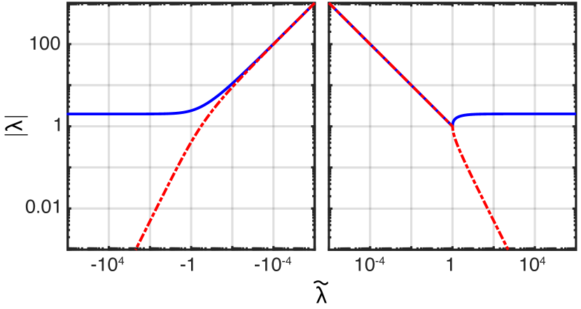
(a) $\widehat{D}_{+}^{-1}$

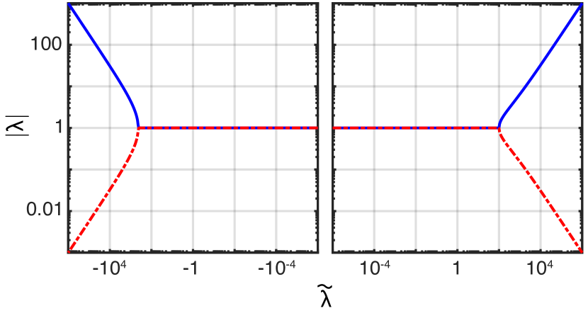
(b) ${D}_{+}^{-1}$

(c) $\widehat{D}_{-}^{-1}$

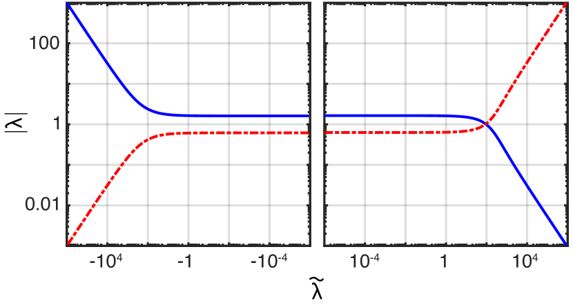
(d) ${D}_{-}^{-1}$

Figure 1: Magnitude of eigenvalue of the preconditioned operator, $|\lambda|$, as a function of a real-valued generalized eigenvalue $\widetilde{\lambda}$ of $(A_{22},S_{22})$, for block-diagonal preconditioners $D_{\pm}^{-1}$ and $\widehat{D}_{\pm}^{-1}$ (Theorem 2.1). All formula for eigenvalues of $D_{\pm}^{-1}A$ and $\widehat{D}_{\pm}^{-1}A$ have a $\pm$ in the definition – solid blue lines correspond to $+$ and dotted red lines correspond to $-$, for the given preconditioner and eigenvalue $\widetilde{\lambda}$.

Here we can see that when $|\widetilde{\lambda}|\lessapprox 100$, $D_{\pm}$ provides a clearly superior preconditioning of eigenvalues than $\widehat{D}_{\pm}$. Conversely, for $|\widetilde{\lambda}|\gtrapprox 1$, $\widehat{D}_{\pm}$ likely provides a comparable or potentially superior preconditioning of eigenvalues. The following example demonstrates how SPD operators may be less amenable to block-diagonal Schur-complement preconditioning.

Example 2.2 (SPD operators).

Suppose $A$ is SPD. Then $A_{11},A_{22}$, and $S_{22}$ are also SPD, and $A_{12}^{T}A_{11}^{-1}A_{12}$ is symmetric positive semi-definite. Notice that $A_{22}^{-1}S_{22}=I-A_{22}^{-1}A_{12}^{T}A_{11}^{-1}A_{12}$, and the eigenvalues of $A_{22}^{-1}A_{12}^{T}A_{11}^{-1}A_{12}$ are real and non-negative. It follows that $\sigma(A_{22}^{-1}S_{22})\subset(0,1]$ and $\widetilde{\lambda}\in\sigma(S_{22}^{-1}A_{22})\subset[1,\infty)$. Looking at Figure 1, eigenvalues of the preconditioned operator are largely outside of the region where a Schur complement provides excellent preconditioning of eigenvalues.

Now let $A_{11},A_{12}$, and $A_{22}$ be random $250\times 250$ matrices uniformly distributed between $[-1,1]$. Then, for positive constants $\{c_{o},c_{1},c_{2}\}$, define

(4) $$M=\begin{bmatrix}A_{11}^{T}A_{11}/c_{1}&A_{12}/c_{o}\\ A_{12}^{T}/c_{o}&A_{22}^{T}A_{22}/c_{2}\end{bmatrix},\hskip 21.52771ptN=\begin{bmatrix}A_{11}^{T}A_{11}/c_{1}&A_{12}/c_{o}\\ A_{12}^{T}/c_{o}&\rho I-A_{22}^{T}A_{22}/c_{2}\end{bmatrix},$$

where $\rho$ is chosen such that $M$ and $N$ have the same minimal magnitude eigenvalue, and $(\rho I-A_{22}^{T}A_{22}/c_{2})\leq 0$. Here $M$ and $N$ are symmetric $500\times 500$ matrices, with SPD (1,1)-block, and SPD or SND (2,2)-block. Table 1 shows the number of block preconditioned GMRES iterations to converge to $10^{-16}$ relative residual tolerance, using a one vector for the right-hand side, and various $\{c_{o},c_{1},c_{2}\}$. Results are shown for block preconditioners $D_{\pm}$, $\widehat{D}_{\pm}$, $L$, and $\widehat{L}$, a lower-triangular preconditioner using $A_{22}$ instead of $S_{22}$.

	$M$						N
$c_{o}/c_{1}/c_{2}$	$L$	$\widehat{L}$	$D_{+}$	$\widehat{D}_{+}$	$D_{-}$	$\widehat{D}_{-}$	$L$	$\widehat{L}$	$D_{+}$	$\widehat{D}_{+}$	$D_{-}$	$\widehat{D}_{-}$
1/1/1	3	167	259	347	276	347	3	122	115	245	101	245
20/1/1	3	36	74	75	74	75	3	33	61	65	60	65
1/10/1	3	434	399	879	416	880	3	343	98	687	88	688
1/10/10	3	501	102	1001	97	1001	3	496	67	995	62	993

Table 1: Block-preconditioned GMRES iterations to $10^{-16}$ relative residual tolerance, with right-hand side $\mathbf{b}=\mathbf{1}$.

From Table 1, note that block-diagonal preconditioning with an exact Schur complement can make for a relatively poor preconditioner (see row 1/1/1). Moreover, for a problem with some sense of block-diagonal dominance (in this case, scaling the off-diagonal blocks by 1/20 compared with diagonal blocks; see row 20/1/1), the exact Schur complement provides almost no improvement over a standard block-diagonal preconditioner, $\widehat{D}_{\pm}$. Last, it is worth pointing out that for all cases, convergence of GMRES is faster applied to $N$ ($A_{22}\leq 0$) than $M$ ($A_{22}\geq 0$), in some cases up to $4\times$ faster, which is generally consistent with Figure 1 and the corresponding discussion.

Finally, we consider how the theory extends to approximate block preconditioners. Consider $N$ with constants $\rho=0$ and $c_{o}/c_{1}/c_{2}=$ 1/10/1 (4), and two (artificial) approximate Schur complements,

$$S_{22}^{*} =A_{22}-(1-\varepsilon_{*})A_{21}A_{11}^{-1}A_{12},\hskip 21.52771ptS_{22}^{\times}=A_{22}-A_{21}A_{11}^{-1}A_{12}+\varepsilon_{\times}E,$$

for error scaling $\varepsilon_{*}\in[0,1],\varepsilon_{\times}\geq 0$. Here, $E$ is a random error matrix with entries uniformly distributed between $[-\eta,\eta]$, where $\eta$ is the average magnitude of entries in $A$. Note that for $\varepsilon_{*}=\varepsilon_{\times}=0$ we have $S_{22}^{*}=S_{22}^{\times}=S_{22}$, while $S_{22}^{*}$ and $S_{22}^{\times}$ generally become decreasingly accurate approximations to $S_{22}$ as $\varepsilon$ increases. Also, $\varepsilon_{*}=1$ yields $S_{22}^{*}=A_{22}$. Then, consider block preconditioners $D_{*},L_{*},D_{\times}$, and $L_{\times}$, which take the form of $D_{+}$ and $L$ in (1), replacing $S_{22}\mapsto S_{22}^{*}$ or $S_{22}\mapsto S_{22}^{\times}$. Figure 2 shows the ratio of block-diagonal to block-lower-triangular preconditioned GMRES iterations to $10^{-16}$ relative residual tolerance, for $S_{22}^{*}$ and $S_{22}^{\times}$, as a function of the corresponding $\varepsilon$ error scaling. Results for $S_{22}^{\times}$ are also shown with $A_{22}=\mathbf{0}$.

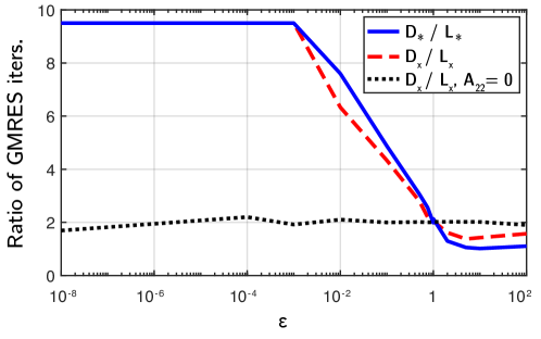
Figure 2: Ratio of block-diagonal to block lower-triangular preconditioned GMRES iterations to $10^{-16}$ relative residual, based on $S_{22}^{*}$ and $S_{22}^{\times}$, as a function of $\varepsilon_{*}$ or $\varepsilon_{\times}$. System matrix $N\in\mathbb{R}^{500\times 500}$ is randomly generated as in (4) with $\rho=0$.

Note that for $\varepsilon\ll 1$ and $A_{22}\neq\mathbf{0}$, $L_{*}$ and $L_{\times}$ are significantly more effective as preconditioners than $D_{*}$ and $D_{\times}$, in both cases requiring $\approx 10\times$ less GMRES iterations (with $L_{*}$ and $L_{\times}$ only requiring $2-4$ iterations). At $\varepsilon_{*}=1$, $S_{22}^{*}=A_{22}$ and, consistent with theory in [20], $D_{*}$ takes almost exactly twice as many iterations as $L_{*}$ (interestingly, the same ratio holds for $D_{\times}/L_{\times}$, although this appears to be coincidence). Finally, for $\varepsilon_{*}>1$, $L_{*}$ takes almost the same number of iterations as $D_{*}$. Despite both being relatively poor preconditioners, this again demonstrates that block-diagonal preconditioning can yield convergence just as fast as block-triangular preconditioning in some cases. Last, for $A_{22}=\mathbf{0}$, we observe the expected result that a block-diagonal preconditioner will require twice as many iterations as block lower-triangular using the same Schur complement approximation, when $A_{22}=\mathbf{0}$ [8].

The above discussion highlights some of the intricacies of Schur-complement preconditioning, and some of the practical insights we can learn from this analysis. An interesting open question is whether the Schur complement is optimal in any sense for block-diagonal preconditioners, or if there is a different “optimal” operator for the (2,2)-block. Of course, optimal in what sense is perhaps the larger question, because as demonstrated in Figure 1 and Table 1 (and generally known [9]), the eigenvalues of the preconditioned operator can all be very nicely bounded, but GMRES can observe arbitrarily slow convergence.

2.2 Proofs

Proof 2.3 (Proof of Theorem 2.1).

The proof is presented as a sequence of lemmas for each preconditioner.

Lemma 2.4 (Spectrum of $D_{+}^{-1}A$).

Proof 2.5.

By nature of the preconditioner, we assume that $A_{11}$ and $S_{22}$ are nonsingular and, thus, so is $A$. Noting the identity $A_{22}=S_{22}+A_{21}A_{11}^{-1}A_{12}$, one can expand $D_{+}^{-1}A$ to the block form

$$D_{+}^{-1}A :=\begin{bmatrix}A_{11}^{-1}&\mathbf{0}\\ \mathbf{0}&{S}_{22}^{-1}\end{bmatrix}\begin{bmatrix}A_{11}&A_{12}\\ A_{21}&A_{22}\end{bmatrix}=\begin{bmatrix}I\\ {S}_{22}^{-1}A_{21}\end{bmatrix}\begin{bmatrix}I&A_{11}^{-1}A_{12}\end{bmatrix}+\begin{bmatrix}\mathbf{0}&\mathbf{0}\\ \mathbf{0}&I\end{bmatrix}.$$

Now consider the corresponding eigenvalue problem,

(5) $$\left(\begin{bmatrix}I\\ {S}_{22}^{-1}A_{21}\end{bmatrix}\begin{bmatrix}I&A_{11}^{-1}A_{12}\end{bmatrix}+\begin{bmatrix}\mathbf{0}&\mathbf{0}\\ \mathbf{0}&I\end{bmatrix}\right)\begin{bmatrix}\mathbf{x}\\ \mathbf{y}\end{bmatrix} =\lambda\begin{bmatrix}\mathbf{x}\\ \mathbf{y}\end{bmatrix},$$

which can be expanded as the set of equations

$$\mathbf{x}+A_{11}^{-1}A_{12}\mathbf{y} =\lambda\mathbf{x},$$

$$S_{22}^{-1}A_{21}(\mathbf{x}+A_{11}^{-1}A_{12}\mathbf{y}) =(\lambda-1)\mathbf{y}.$$

If $A_{12}$ or $A_{21}$ are not full rank, then for each $\mathbf{y}_{k}\in$ ker$(A_{12})$ or each $\mathbf{x}_{k}\in$ ker$(A_{21})$, there exist eigenpairs $\left\{[\mathbf{0};\mathbf{y}_{k}],1\right\}$ or $\left\{[\mathbf{x}_{k};\mathbf{0}],1\right\}$, respectively (the ; denotes a column vector). This accounts for dim(ker($A_{21}))+$ dim(ker($A_{12}))$ eigenvalues. For $\mathbf{x}\not\in$ ker$(A_{21})$ and $\mathbf{y}\not\in$ ker$(A_{12})$, solving for $\mathbf{x}$ yields $\mathbf{x}:=\frac{-1}{1-\lambda}A_{11}^{-1}A_{12}\mathbf{y}$. Plugging in reduces (5) to an eigenvalue problem for $\mathbf{y}$,

(6) $$S_{22}^{-1}A_{21}A_{11}^{-1}A_{12}\mathbf{y} =\frac{(1-\lambda)^{2}}{\lambda}\mathbf{y}.$$

Let $\widehat{\lambda}:=(1-\lambda)^{2}/\lambda$ and assume $\lambda\neq 1$. Expanding, we have $\lambda^{2}-\lambda(2+\widehat{\lambda})+1=0$, and solving for $\lambda$ yields $\lambda=1+\frac{\widehat{\lambda}}{2}\pm\frac{1}{2}\sqrt{\widehat{\lambda}(\widehat{\lambda}+4)}$.

Now consider the eigenvalue problem in (6) for $\widehat{\lambda}$. Applying $S_{22}$ to both sides and rearranging yields the generalized eigenvalue problem $A_{22}\mathbf{y}=\frac{1+\widehat{\lambda}}{\widehat{\lambda}}A_{21}A_{11}^{-1}A_{12}\mathbf{y}$. Subtracting $\frac{1+\widehat{\lambda}}{\widehat{\lambda}}A_{22}$ from both sides then yields the equivalent generalized eigenvalue problem

(7) $$A_{22}\mathbf{y} =(1+\widehat{\lambda})S_{22}\mathbf{y}.$$

Thus, let $\widetilde{\lambda}$ be a generalized eigenvalue of $(A_{22},S_{22})$ in (7). Solving for $\widehat{\lambda}$ yields $\widehat{\lambda}:=(\widetilde{\lambda}-1)$ as a function of generalized eigenvalues of $(A_{22},S_{22})$ (note, for $\mathbf{y}\in$ ker$(A_{22})$, we have $\widehat{\lambda}=-1$). Furthermore, the generalized eigenvectors in (7) are the same as eigenvectors in the (2,2)-block for the preconditioned operator (5). Plugging $\widehat{\lambda}$ into the equation above for $\lambda$, we can express the eigenvalues and eigenvectors of $D_{+}^{-1}A$ as a nonlinear function of the generalized eigenvalues of $(A_{22},S_{22})$,

(8) $$\sigma(D_{+}^{-1}A)=\left(\frac{\widetilde{\lambda}+1}{2}\pm\frac{1}{2}\sqrt{(\widetilde{\lambda}-1)(\widetilde{\lambda}+3)}\right)\quad\mathbin{\scalebox{1.5}{$\cup$}}\quad\left\{1\right\},$$

Eigenvectors of the former set in (8) are given by $[\frac{-1}{1-\lambda}A_{11}^{-1}A_{12}\mathbf{y};\mathbf{y}]$ for each generalized eigenpair $\{\mathbf{y},\widehat{\lambda}\}$ of (7) and eigenvalue $\lambda(\widehat{\lambda})$. Note that each generalized eigenpair of $(A_{22},S_{22})$ corresponds to two eigenpairs of $D_{+}^{-1}A$, because $\lambda(\widehat{\lambda})=0$ is a quadratic equation in $\lambda$. The latter eigenvalue $\lambda=1$ in (8) has multiplicity given by the sum of dimensions of ker$(A_{12})$ and ker$(A_{21}$, with eigenvectors as defined previously in the proof.

Lemma 2.6 (Spectrum of $D_{-}^{-1}A$).

Proof 2.7.

The proof proceed analogous to Lemma 2.4. The block-preconditioned eigenvalue problem can be expressed as the set of equations

$$\mathbf{x}+A_{11}^{-1}A_{12}\mathbf{y} =\lambda\mathbf{x},$$

$$-S_{22}^{-1}A_{21}(\mathbf{x}+A_{11}^{-1}A_{12}\mathbf{y}) =(\lambda+1)\mathbf{y}.$$

If $A_{12}$ or $A_{21}$ are not full rank, then for each $\mathbf{y}_{k}\in$ ker$(A_{12})$ or each $\mathbf{x}_{k}\in$ ker$(A_{21})$, there exist eigenpairs $\left\{[\mathbf{0};\mathbf{y}_{k}],-1\right\}$ or $\left\{[\mathbf{x}_{k};\mathbf{0}],1\right\}$, respectively. This accounts for dim(ker($A_{21}))+$ dim(ker($A_{12}))$ eigenvalues. For $\mathbf{x}\not\in$ ker$(A_{21})$ and $\mathbf{y}\not\in$ ker$(A_{12})$, solving for $\mathbf{x}$ yields $\mathbf{x}:=\frac{-1}{1-\lambda}A_{11}^{-1}A_{12}\mathbf{y}$. Plugging in reduces to an eigenvalue problem for $\mathbf{y}$,

(9) $$S_{22}^{-1}A_{21}A_{11}^{-1}A_{12}\mathbf{y} =\frac{(1-\lambda)(1+\lambda)}{\lambda}\mathbf{y}.$$

Let $\widehat{\lambda}:=(1-\lambda)(1+\lambda)/\lambda$ and assume $\lambda\neq\pm 1$. Expanding, we have $\lambda^{2}+\lambda\widehat{\lambda}-1=0$, and solving for $\lambda$ yields $\lambda=-\frac{\widehat{\lambda}}{2}\pm\frac{1}{2}\sqrt{\widehat{\lambda}^{2}+4}$. Plugging $\widehat{\lambda}:=\widetilde{\lambda}-1$ as in Lemma 2.4 yields the spectrum of $D_{-}^{-1}A$ as a nonlinear function of the generalized eigenvalues of $(A_{22},S_{22})$,

(10) $$\sigma({D}_{-}^{-1}A)=\left(-\frac{\widetilde{\lambda}-1}{2}\pm\frac{1}{2}\sqrt{(\widetilde{\lambda}-1)^{2}+4}\right)\quad\mathbin{\scalebox{1.5}{$\cup$}}\quad\left\{\pm 1\right\}.$$

Eigenvectors of the former set in (10) are given by $[\frac{-1}{1-\lambda}A_{11}^{-1}A_{12}\mathbf{y};\mathbf{y}]$ for each generalized eigenpair $\{\mathbf{y},\widehat{\lambda}\}$ of (7) and eigenvalue $\lambda(\widehat{\lambda})$. Note that each generalized eigenpair of $(A_{22},S_{22})$ corresponds to two eigenpairs of $D_{+}^{-1}A$, because $\lambda(\widehat{\lambda})=0$ is a quadratic equation in $\lambda$. The latter eigenvalues $\lambda=-1$ and $\lambda=1$ in (10) have multiplicity given by dimensions of ker$(A_{12})$ and ker$(A_{21})$, respectively, with eigenvectors as defined previously in the proof.

Lemma 2.8 (Spectrum of $\widehat{D}_{+}^{-1}A$).

Proof 2.9.

Observe

$$\widehat{D}_{+}^{-1}A =\begin{bmatrix}A_{11}^{-1}&\mathbf{0}\\ \mathbf{0}&A_{22}^{-1}\end{bmatrix}\begin{bmatrix}A_{11}&A_{12}\\ A_{21}&A_{22}\end{bmatrix}=I+\begin{bmatrix}\mathbf{0}&A_{11}^{-1}A_{12}\\ A_{22}^{-1}A_{21}&\mathbf{0}\end{bmatrix}.$$

with eigenvalues and eigenvectors determined by the off-diagonal matrix on the right. If $A_{12}$ or $A_{21}$ are not full rank, then for each $\mathbf{y}_{k}\in$ ker$(A_{12})$ or each $\mathbf{x}_{k}\in$ ker$(A_{21})$, there exist eigenpairs $\left\{[\mathbf{0};\mathbf{y}_{k}],1\right\}$ or $\left\{[\mathbf{x}_{k};\mathbf{0}],1\right\}$, respectively. For $\mathbf{x}\not\in$ ker$(A_{21})$ and $\mathbf{y}\not\in$ ker$(A_{12})$, we consider eigenvalues of the off-diagonal matrix in (2.9). Squaring this matrix results in the block-diagonal eigenvalue problem

(11) $$\begin{bmatrix}A_{11}^{-1}A_{12}A_{22}^{-1}A_{21}&\mathbf{0}\\ \mathbf{0}&A_{22}^{-1}A_{21}A_{11}^{-1}A_{12}\end{bmatrix}\begin{bmatrix}\mathbf{x}\\ \mathbf{y}\end{bmatrix} =\widehat{\lambda}\begin{bmatrix}\mathbf{x}\\ \mathbf{y}\end{bmatrix}.$$

We can restrict ourselves to the case of $\mathbf{x}\not\in$ ker$(A_{21})$ and $\mathbf{y}\not\in$ ker$(A_{12})$. Note by similarity that the spectrum of $A_{22}^{-1}A_{21}A_{11}^{-1}A_{12}$ is equivalent to that of $A_{21}A_{11}^{-1}A_{12}A_{22}^{-1}$. Now suppose $A_{11}^{-1}A_{12}A_{22}^{-1}A_{21}\mathbf{x}=\lambda\mathbf{x}$, and let $\mathbf{w}:=A_{21}\mathbf{x}$. Then $A_{21}A_{11}^{-1}A_{12}A_{22}^{-1}\mathbf{w}=A_{21}(A_{11}^{-1}A_{12}A_{22}^{-1}A_{12}\mathbf{x})=\lambda A_{21}\mathbf{x}=\lambda\mathbf{w}$. Thus if $\{\lambda,\mathbf{x}\}$ is a nonzero eigenpair of $A_{11}^{-1}A_{12}A_{22}^{-1}A_{21}$, then $\{\lambda,A_{22}^{-1}A_{21}\mathbf{x}\}$ is an eigenpair of $A_{22}^{-1}A_{21}A_{11}^{-1}A_{12}$. To that end, eigenvalues of (11) consist of 0, corresponding to the kernels of $A_{21}$ and $A_{12}$, and the nonzero eigenvalues of the lower diagonal block (or upper), all with multiplicity two.

Now note that $A_{22}^{-1}A_{21}A_{11}^{-1}A_{12}=I-A_{22}^{-1}S_{22}$, and let $\widetilde{\lambda}$ be a generalized eigenvalue of $(S_{22},A_{22})$. Then, $\widehat{\lambda}=1-\widetilde{\lambda}$, and the spectrum of $D_{-}^{-1}A$ can be written as a nonlinear function of the generalized eigenvalues of $(S_{22},A_{22})$,

$$\sigma(\widehat{D}_{+}^{-1}A) =\left(1\pm\sqrt{1-\widetilde{\lambda}}\right)\quad\mathbin{\scalebox{1.5}{$\cup$}}\quad\left\{\pm 1\right\},$$

with inclusion of the latter set of eigenvalues depending on the rank of $A$ and $A_{12}$/$A_{21}$, respectively.

Note, each vector $\mathbf{v}_{k}\in$ ker$(A)$ correspond to a $\mathbf{y}_{k}\in$ ker$(S_{22})$. In the context of the generalized eigenvalues of $(S_{22},A_{22})$, each $\widetilde{\lambda}=0$ is one-to-one with an eigenvalue $\lambda=0$ of $\widehat{D}_{+}^{-1}A$, which can be seen by plugging $\widetilde{\lambda}=0$ into (2.9).

Lemma 2.10 (Spectrum of $\widehat{D}_{-}^{-1}A$).

Proof 2.11.

Observe

(12) $$\widehat{D}_{-}^{-1}A =\begin{bmatrix}A_{11}^{-1}&\mathbf{0}\\ \mathbf{0}&-A_{22}^{-1}\end{bmatrix}\begin{bmatrix}A_{11}&A_{12}\\ A_{21}&A_{22}\end{bmatrix}=-I+\begin{bmatrix}2I&A_{11}^{-1}A_{12}\\ -A_{22}^{-1}A_{21}&\mathbf{0}\end{bmatrix},$$

with eigenvalues and eigenvectors determined by the saddle-point matrix on the right. If $A_{12}$ or $A_{21}$ are not full rank, then for each $\mathbf{y}_{k}\in$ ker$(A_{12})$ or each $\mathbf{x}_{k}\in$ ker$(A_{21})$, there exist eigenpairs $\left\{[\mathbf{0};\mathbf{y}_{k}],-1\right\}$ or $\left\{[\mathbf{x}_{k};\mathbf{0}],1\right\}$, respectively. For $\mathbf{x}\not\in$ ker$(A_{21})$ and $\mathbf{y}\not\in$ ker$(A_{12})$, analogous to Lemma 2.4 we can formulate an eigenvalue problem for the saddle-point matrix, with eigenvalue $\widehat{\lambda}$ and block eigenvector $[\mathbf{x};\mathbf{y}]$. Solving for $\mathbf{x}=\frac{1}{\widehat{\lambda}-2}A_{11}^{-1}A_{12}\mathbf{y}$ and plugging into the equation for $\mathbf{y}$ yields an equivalent reduced eigenvalue problem,

(13) $$A_{22}^{-1}A_{21}A_{11}^{-1}A_{12}\mathbf{y} =\widehat{\lambda}(2-\widehat{\lambda})\mathbf{y}.$$

Note, this is well-posed in the sense that we only care about $\mathbf{y}\not\in$ ker$(A_{12})$ and $\mathbf{x}=\frac{1}{\widehat{\lambda}-2}A_{11}^{-1}A_{12}\mathbf{y}\not\in$ ker$(A_{21})$. Noting that $A_{22}^{-1}A_{21}A_{11}^{-1}A_{12}=I-A_{22}^{-1}S_{22}$, (13) is equivalent to the generalized eigenvalue problem

(14) $$S_{22}\mathbf{y} =(1-\widehat{\lambda})^{2}A_{22}\mathbf{y}.$$

Letting $\widetilde{\lambda}$ be a generalized eigenvalue of $(S_{22},A_{22})$ in (14) and solving for $\widehat{\lambda}$ yields $\widehat{\lambda}=1\pm\sqrt{\widetilde{\lambda}}$. Including the minus identity perturbation in (12) yields the spectrum of $D_{-}^{-1}A$ as a nonlinear function of the generalized eigenvalues of $(S_{22},A_{22})$ in (14), given by

$$\sigma(\widehat{D}_{-}^{-1}A)=\left(\pm\sqrt{\widetilde{\lambda}}\right)\quad\mathbin{\scalebox{1.5}{$\cup$}}\quad\left\{\pm 1\right\},$$

Eigenvectors corresponding to eigenvalues $\sqrt{\widetilde{\lambda}}$ are given by $[\frac{-1}{1-\lambda}A_{11}^{-1}A_{12}\mathbf{y};\mathbf{y}]$ for each generalized eigenpair $\{\mathbf{y},\widehat{\lambda}\}$ of (7) and eigenvalue $\lambda(\widehat{\lambda})$. Note that each generalized eigenpair of $(S_{22},A_{22})$ corresponds to two eigenpairs of $\widehat{D}_{-}^{-1}A$, because $\lambda(\widehat{\lambda})=0$ is a quadratic equation in $\lambda$. The latter eigenvalue $\lambda=1$ in (8) has multiplicity given by the sum of dimensions of ker$(A_{12})$ and ker$(A_{21}$, with eigenvectors as defined previously in the proof.

3 Applications in transport: $\mathcal{H}_{1}\otimes L_{2}$ VEF

3.1 The variable Eddington factor (VEF) method

The steady-state, mono-energetic, discrete-ordinates, linear Boltzmann equation with isotropic scattering and source is given by

(15) $$\boldsymbol{\Omega}_{d}\cdot\nabla\psi_{d}(\boldsymbol{\mathrm{x}})+\sigma_{t}(\boldsymbol{\mathrm{x}})\psi_{d}(\boldsymbol{\mathrm{x}}) =\frac{\sigma_{s}(\boldsymbol{\mathrm{x}})}{4\pi}\sum_{d^{\prime}=1}^{N}w_{d^{\prime}}\psi_{d^{\prime}}(\boldsymbol{\mathrm{x}})+\frac{Q(\boldsymbol{\mathrm{x}})}{4\pi}\,,\quad\boldsymbol{\mathrm{x}}\in\mathcal{D}\,,$$

$$\psi_{d}(\boldsymbol{\mathrm{x}}) =\overline{\psi}(\boldsymbol{\mathrm{x}},\boldsymbol{\Omega}_{d})\,,\quad\boldsymbol{\mathrm{x}}\in\partial\mathcal{D}\ \mathrm{and}\ \boldsymbol{\Omega}_{d}\cdot\boldsymbol{\mathrm{n}}<0\,.$$

Here, the direction of particle motion, $\boldsymbol{\Omega}$, is discretized into $N$ angles corresponding to a quadrature rule for the unit sphere, $\{\boldsymbol{\Omega}_{d},w_{d}\}_{d=1}^{N}$, for quadrature weights $w_{d}>0$. A standard approach to solve (15) is to (independently) invert the left-hand side for each $\psi_{d}$, update $\sum_{d^{\prime}=1}^{N}w_{d^{\prime}}\psi_{d^{\prime}}(\boldsymbol{\mathrm{x}})$, and repeat until convergence. Unfortunately, for many applications of interest, this process can converge arbitrarily slowly.

An alternative scheme for solving (15) is the Variable Eddington factor (VEF) method, a nonlinear iterative scheme that builds an exact reduced-order model of the transport equation [21, 6]. The VEF reduced-order model is given by

(16) $$\begin{split}\nabla\cdot\boldsymbol{\mathrm{J}}(\boldsymbol{\mathrm{x}})+\sigma_{a}(\boldsymbol{\mathrm{x}})\varphi(\boldsymbol{\mathrm{x}})&=Q(\boldsymbol{\mathrm{x}})\,\\ \nabla\cdot\left[\boldsymbol{\mathrm{E}}(\boldsymbol{\mathrm{x}})\varphi(\boldsymbol{\mathrm{x}})\right]+\sigma_{t}(\boldsymbol{\mathrm{x}})\boldsymbol{\mathrm{J}}(\boldsymbol{\mathrm{x}})&=0\,.\end{split}$$

It is derived by taking the zeroth and first angular moments of (15), and introducing the Eddington tensor as a closure:

(17) $$\boldsymbol{\mathrm{E}}(\boldsymbol{\mathrm{x}})=\frac{\sum_{d=1}^{N}\boldsymbol{\Omega}_{d}\otimes\boldsymbol{\Omega}_{d}\,\psi_{d}(\boldsymbol{\mathrm{x}})w_{d}}{\sum_{d=1}^{N}\psi_{d}(\boldsymbol{\mathrm{x}})w_{d}}\,.$$

The algorithm is then to replace the scattering sum $\sum_{d^{\prime}=1}^{N}w_{d^{\prime}}\psi_{d^{\prime}}(\boldsymbol{\mathrm{x}})$ in (15) with the solution of the VEF equations, $\varphi(\boldsymbol{\mathrm{x}})$, invert (15) for each angle, update the Eddington tensor, and solve the VEF equations.

Here we consider an $\mathcal{H}^{1}(\mathcal{D})\otimes L^{2}(\mathcal{D})$ mixed finite element discretization of (16), as in [14, 13]. This yields the $2\times 2$ block system

(18) $$\begin{bmatrix}M_{t}&-G\\ B&M_{a}\end{bmatrix}\begin{bmatrix}\boldsymbol{\mathrm{J}}\\ \boldsymbol{\mathrm{\varphi}}\end{bmatrix}=\begin{bmatrix}\boldsymbol{\mathrm{g}}\\ \boldsymbol{\mathrm{f}}\end{bmatrix}\,,$$

where $M_{t}$ is an $\mathcal{H}^{1}(\mathcal{D})$ mass matrix, $M_{a}$ a (block diagonal) $L^{2}(\mathcal{D})$ mass matrix, $B$ the $L^{2}(\mathcal{D})\otimes\mathcal{H}^{1}(\mathcal{D})$ divergence matrix, and $G$ the $\mathcal{H}^{1}(\mathcal{D})\otimes L^{2}(\mathcal{D})$ Eddington gradient matrix, defined as $\boldsymbol{\mathrm{v}}^{T}G\boldsymbol{\mathrm{\varphi}}=\int_{\mathcal{D}}\nabla\boldsymbol{\mathrm{v}}:\boldsymbol{\mathrm{E}}\varphi\,d\boldsymbol{\mathrm{x}}$. Note that for $\sigma_{a}(x)=\sigma_{t}(x)-\sigma_{s}(x)=0$, $M_{a}=\mathbf{0}$ and (18) simplifies to a saddle-point system with zero (2,2)-block. Due to the Eddington tensor, $B\neq-G^{T}$ and, thus, at every VEF iteration a non-symmetric $2\times 2$ block operator of the form in (1) must be solved.

3.2 Solution of $\mathcal{H}_{1}\otimes L_{2}$ VEF discretization

There are a number of advantages to VEF over other methods of solving (15) [14, 13], but the system in (18) remains difficult to solve. However, because the diagonal blocks of (18) are mass matrices and relatively easy to invert, direct application or preconditioning of the Schur complement, $S_{22}:=M_{a}+BM_{t}^{-1}G$, is feasible, which corresponds to a drift-diffusion-like equation. The remaining challenge is that $M_{t}$ is an $\mathcal{H}^{1}(\mathcal{D})$ mass matrix and, although the action of $M_{t}^{-1}$ can be computed rapidly using Krylov methods, a closed form to construct $S_{22}:=M_{a}+BM_{t}^{-1}G$ is typically not available. A common solution is to approximate $M_{t}$ using quadrature lumping, resulting in a diagonal approximation, $\widetilde{M}_{t}$. Thus, consider the four preconditioners,

(19) $$\begin{split}D&=\begin{bmatrix}M_{t}&\mathbf{0}\\ \mathbf{0}&M_{a}+BM_{t}^{-1}G\end{bmatrix},\hskip 24.75687ptL=\begin{bmatrix}M_{t}&\mathbf{0}\\ B&M_{a}+BM_{t}^{-1}G\end{bmatrix},\\ \widetilde{D}&=\begin{bmatrix}M_{t}&\mathbf{0}\\ \mathbf{0}&M_{a}+B\widetilde{M_{t}}^{-1}G\end{bmatrix}\,,\hskip 21.52771pt\widetilde{L}=\begin{bmatrix}M_{t}&\mathbf{0}\\ B&M_{a}+B\widetilde{M_{t}}^{-1}G\end{bmatrix}.\end{split}$$

Consider a 1d discretization of (16), where $\mathrm{J}$ is discretized with quadratic $\mathcal{H}^{1}(\mathcal{D})$ and $\varphi$ with linear $L^{2}(\mathcal{D})$, with $\sigma_{t}(x)=Q(x)=1$ and absorption $\sigma_{a}\in\{0,0.9\}$ to demonstrate the effect of the $A_{22}$ block ($A_{22}=\mathbf{0}$ when $\sigma_{a}=0$). In the limit of $\sigma_{t}\gg 1$, $E\to\frac{1}{3}I$, wherein scaling the second row of (18) by $-1/3$ then results in a symmetric operator. Although this is unlikely to occur on the whole domain in practice, we perform tests on this case as well to demonstrate that results do not depend on nonsymmetry in (18). Table 2 shows the number of GMRES iterations to converge to $10^{-10}$ relative residual tolerance using block preconditioners in (19).

							Unlumped	Lumped
	$\sigma_{a}$	$N$	Diagonal	Triangular	Diagonal	Triangular
Nonsymm.	0	401	2	2	44	23
	0	4001	4	4	53	25
	0.9	401	12	2	57	27
	0.9	4001	12	4	77	32
Symm.	0	401	2	2	44	23
	0	4001	4	4	55	25
	0.9	401	12	2	57	27
	0.9	4001	12	4	76	26

Table 2:

The unlumped block-diagonal and triangular preconditioners converge in two or four iterations when the $A_{22}$ block is zero, largely consistent with theory in [11, 10]. However, when $M_{a}=A_{22}\neq\mathbf{0}$, block-diagonal preconditioning requires 12 iterations. Although this is better than the several hundred seen in Table 1, it is still $3-6\times$ slower than block lower triangular. Moreover, the example problem used here is relatively simple and one-dimensional – initial experiments on harder problems have required a larger number of iterations. We can also see how sensitive Schur-complement preconditioning can be to approximations, where the lumped preconditioners increase iteration counts by $10\times$ or more. In practice, lumping $M_{t}$ is likely necessary because we cannot directly form $M_{a}+BM_{t}^{-1}G$, which makes construction of effective preconditioners difficult. Considering this problem in the context of Schur-complement preconditioning has suggested reformulating (18) using a lumped $M_{t}$ (which we can solve in $\approx 2$ iterations), block-triangular preconditioners, and handling the difference between a lumped and non-lumped $M_{t}$ in the larger nonlinear VEF iteration. This is ongoing work, and an interesting application of Schur-complement preconditioning.

4 Conclusions

The simple lesson from Section 3 is that implementing a block-triangular (or block-LDU if symmetry is important) preconditioner may provide a significant speedup over block-diagonal preconditioners ($\ll 1/2$ the iteration count), and should be considered in practice for $A_{22}\neq\mathbf{0}$ and Schur-complement approximation $\widehat{S}_{22}\neq A_{22}$. The larger point of this paper is that which type of block preconditioner to use is largely problem specific, and should be considered on a case-by-case basis. When $A_{22}=\mathbf{0}$, it is generally known that block-diagonal preconditioners will require roughly twice as many minimal-residual iterations to converge as block-triangular or block-LDU [8], and it is straightforward to estimate the associated computational costs for each preconditioner and pick the most efficient choice. For $A_{22}\neq\mathbf{0}$, examples in Section 2.1 demonstrate that block-diagonal and block-triangular preconditioning can converge in a similar or very different number of iterations. Another recently developed $2\times 2$ block preconditioner for transport problems found that the block-triangular variation rarely showed any reduction in iteration count over block-diagonal, while computing the action of the off-diagonal blocks made the triangular variation several times more expensive [19]. In that case, implementing the triangular variation is also non-trivial, and the block-diagonal preconditioner is clearly superior in terms of performance and ease of implementation.

References

- [1] Z. Z. Bai and M. K. Ng, On Inexact Preconditioners for Nonsymmetric Matrices, SIAM Journal on Scientific Computing, 26 (2005), pp. 1710–1724.
- [2] Z. Z. Bai, M. K. Ng, and Z.-Q. Wang, Constraint Preconditioners for Symmetric Indefinite Matrices, SIAM Journal on Matrix Analysis and Applications, 31 (2009), pp. 410–433.
- [3] M. Benzi, G. H. Golub, and J. Liesen, Numerical solution of saddle point problems, Acta Numerica, 14 (2005), pp. 1–137.
- [4] Z.-H. Cao, A note on constraint preconditioning for nonsymmetric indefinite matrices, SIAM Journal on Matrix Analysis and Applications, 24 (2003), pp. 121–125.
- [5] Z.-H. Cao, A note on spectrum distribution of constraint preconditioned generalized saddle point matrices, Numerical Linear Algebra with Applications, 16 (2009), pp. 503–516.
- [6] D. Mihalas, Stellar Atmospheres, W. H. Freeman and Co, 1978.
- [7] E. de Sturler and J. Liesen, Block-Diagonal and Constraint Preconditioners for Nonsymmetric Indefinite Linear Systems. Part I: Theory, SIAM Journal on Scientific Computing, 26 (2005), pp. 1598–1619.
- [8] B. Fischer, A. Ramage, D. J. Silvester, and A. J. Wathen, Minimum residual methods for augmented systems, BIT, 38 (1998), pp. 527–543.
- [9] A. Greenbaum, V. Pt ’ak, and Z. Strako u s, Any nonincreasing convergence curve is possible for GMRES, SIAM Journal on Matrix Analysis and Applications, 17 (1996), pp. 465–469.
- [10] I. C. F. Ipsen, A note on preconditioning nonsymmetric matrices, SIAM Journal on Scientific Computing, 23 (2001), pp. 1050–1051.
- [11] M. F. Murphy, G. H. Golub, and A. Wathen, A note on preconditioning for indefinite linear systems, SIAM Journal on Scientific Computing, 21 (2000), pp. 1969–1972.
- [12] Y. Notay, A New Analysis of Block Preconditioners for Saddle Point Problems, SIAM Journal on Matrix Analysis and Applications, 35 (2014), pp. 143–173.
- [13] S. S. Olivier, P. G. Maginot, and T. S. Haut, High order mixed finite element discretization for the variable eddington factor equations.
- [14] S. S. Olivier and J. E. Morel, Variable eddington factor method for the sn equations with lumped discontinuous galerkin spatial discretization coupled to a drift-diffusion acceleration equation with mixed finite-element discretization, Journal of Computational and Theoretical Transport, 46 (2017), pp. 480–496.
- [15] C. C. Paige and M. A. Saunders, Solution of Sparse Indefinite Systems of Linear Equations, SIAM Journal on Numerical Analysis, 12 (1975), pp. 617–629.
- [16] J. Pestana, On the Eigenvalues and Eigenvectors of Block Triangular Preconditioned Block Matrices, SIAM Journal on Matrix Analysis and Applications, 35 (2014), pp. 517–525.
- [17] Y. Saad and M. H. Schultz, GMRES: A generalized minimal residual algorithm for solving nonsymmetric linear systems, SIAM Journal on scientific and statistical computing, 7 (1986), pp. 856–869.
- [18] C. Siefert and E. de Sturler, Preconditioners for Generalized Saddle-Point Problems, SIAM Journal on Numerical Analysis, 44 (2006), pp. 1275–1296.
- [19] B. S. Southworth, M. Holec, and T. S. Haut, Diffusion synthetic acceleration for heterogeneous domains, compatible with voids, (in review), (2019).
- [20] B. S. Southworth, A. A. Sivas, and S. Rhebergen, On fixed-point, krylov, and block preconditioners, arXiv preprint arXiv:1911.02664, (2019).
- [21] V. Ya. Gol’din, A quasi-diffusion method of solving the kinetic equation, USSR Comp. Math. and Math. Physics, 4 (1964), pp. 136–149.
- [22] A. J. Wathen, Preconditioning, Acta Numerica, 24 (2015), pp. 329–376.