On Symmetric Gauss-Seidel ADMM Algorithm
for $\mathcal{H}_{\infty}$ Guaranteed Cost Control with
Convex Parameterization

Abstract

This paper involves the innovative development of a symmetric Gauss-Seidel ADMM algorithm to solve the $\mathcal{H}_{\infty}$ guaranteed cost control problem. In the presence of parametric uncertainties, the $\mathcal{H}_{\infty}$ guaranteed cost control problem generally leads to the large-scale optimization. This is due to the exponential growth of the number of the extreme systems involved with respect to the number of parametric uncertainties. In this work, through a variant of the Youla-Kucera parameterization, the stabilizing controllers are parameterized in a convex set; yielding the outcome that the $\mathcal{H}_{\infty}$ guaranteed cost control problem is converted to a convex optimization problem. Based on an appropriate re-formulation using the Schur complement, it then renders possible the use of the ADMM algorithm with symmetric Gauss-Seidel backward and forward sweeps. Significantly, this approach alleviates the often-times prohibitively heavy computational burden typical in many $\mathcal{H}_{\infty}$ optimization problems while exhibiting good convergence guarantees, which is particularly essential for the related large-scale optimization procedures involved. With this approach, the desired robust stability is ensured, and the disturbance attenuation is maintained at the minimum level in the presence of parametric uncertainties. Rather importantly too, with the attained effectiveness, the methodology thus evidently possesses extensive applicability in various important controller synthesis problems, such as decentralized control, sparse control, and output feedback control problems.

I Introduction

Robust control theory typically investigates the effect of disturbances, noises, and uncertainties on system performance; and continued great efforts have been devoted to robust stabilization and robust performance in the literature [1, 2, 3, 4, 5, 6, 7]. Quite remarkably, several significant results [8, 9, 10] have been reported which relate the notion of quadratic stabilization to robust stabilization for a class of uncertain linear systems, and by this concept, the stability of an uncertain system is established with a quadratic Lyapunov function. On the other hand, it is also the case that $\mathcal{H}_{\infty}$ control is commonly and extensively used to attenuate the effect of disturbances on the system performance [11, 12]. Additionally, it is further known and shown in [13] that a certain type of quadratic stabilization problem can be essentially expressed as an $\mathcal{H}_{\infty}$ control problem, where a Riccati inequality condition relates the determination of a stabilizing feedback gain that imposes a suitable $\gamma$ disturbance attenuation level [14, 15]. Also notably, the problem of finding the minimal disturbance attenuation level is recognized as an important and commonly-encountered problem, and stated as the optimal $\mathcal{H}_{\infty}$ control problem. On this, it is additionally noteworthy that the work in [16] shows that the problem can be tackled by an iterative algorithm based on the Riccati inequality condition. However here, nonlinear characteristics of the Riccati inequality condition typically result in significant complexity and difficulty in obtaining the optimal gain and disturbance attenuation level. Moreover, $\mathcal{H}_{\infty}$ filtering has been widely studied for state estimation [17, 18]. It is remarkable that $\mathcal{H}_{\infty}$ filtering allows the system disturbances to be unknown, and uncertainties are tolerated in the system.

As considerable efforts have been made on the well-known Youla-Kucera parameterization (also known as $Q$-parameterization) for the determination of stabilizing controllers [19, 20, 21], one may thus think about borrowing this idea to solve the $\mathcal{H}_{\infty}$ optimal control problem in the presence of parametric uncertainties. However, the derivations of the classical Youla-Kucera parameterization results rely on the fact that the plant is linear with no parametric uncertainty, and the order of the controller depends on the order of the plant model and that of $Q$. Alternative parameterization techniques based on the positive real lemma and the bounded real lemma [22, 23] have also been proposed to deal with parametric uncertainties. However, as the required transfer function representation there results in reduced stability in numerical computations, and high computational cost also incurs; it is not considered as a preferable choice for many practical applications. Hence, several other parameterization methods are presented instead in a state-space framework, for example [24]. In essence, these techniques are considered as variants of the Youla-Kucera parameterization, but with more flexibility to deal with the structural constraints and parametric uncertainties. Regarding the nonlinear constraints existing in such a parameterization (also noted to be convex in [24]), outer linearization is necessary for polyhedral approximation during iterative refinement [25]. Similarly, the cutting-plane method is presented in [26, 27] to solve generalized $\mathcal{H}_{\infty}$ control problems. This technique could be effective in some scenarios, but there could be other certain scenarios such as high-dimension systems or uncertain systems with a large volume of parametric uncertainties. For example, in [28], a large-scale $\mathcal{H}_{\infty}$ optimal control problem is simplified in a way that enables sparse solutions and efficient computation. In [29], a distributed $\mathcal{H}_{\infty}$ controller is developed for large-scale platoons. In the scenarios that high-dimension optimization is involved (which resulted from rather numerous extreme systems involved computationally), the convergence rate of the cutting-plane method can be unacceptably slow; and in some cases, the optimization process could even terminate abruptly with unsuccessful outcomes. This is because a sizeable number of cutting planes needs to be added computationally at each iteration, and in difficult scenarios, the optimization process can thus become unwieldy. It is also worth mentioning that this method can only guarantee the so-called $\epsilon$-optimality because the constraints are typically not exactly satisfied but violated by certain small values. Therefore, such a situation causes deviations from the “true" optimal result, and consequently the desired robustness is not perfectly guaranteed, and particularly so if the parametric uncertainties are significant.

Because of the typical computational burden arising from the growth of system dimensions and parametric uncertainties, several advanced optimization techniques are presented in the more recent works. Hence for large-scale and nonlinear optimization problems, the alternating direction method of multipliers (ADMM) [30, 31, 32, 33] has attracted considerable attention from researchers, and is widely used in various areas such as statistical learning [30], distributed computation [34, 35, 36], and multi-agent systems [37, 38]. ADMM demonstrates high efficiency in the determination of the optimal solution to many challenging problems. Remarkably too, some of these challenging optimization problems cannot even be solved by the existing conventional gradient-based approaches, and in these, ADMM demonstrates its superiority. Nevertheless, the conventional ADMM methodology only ensures appropriate convergence with utilization of a two-block optimization structure, and this constraint renders a serious impediment to practical execution [39]. To cater to this deficiency, the symmetric Gauss-Seidel technique can be used to conduct the ADMM optimization serially [40, 41], which significantly improves the feasibility of the ADMM in many large-scale optimization problems. Although these methodologies are reasonably well-established, nevertheless only rather generic procedures are given at the present stage. Therefore, it leaves an open problem on how to apply these advanced optimization techniques in control problems such that these methodologies can be extended beyond the theoretical level.

It is also rather essential at this point to note that in the presence of significant parametric uncertainties, the $\mathcal{H}_{\infty}$ optimization problem is usually of the large-scale type (because of the exponential growth of the number of extreme systems involved computationally with respect to the number of parametric uncertainties; and each of these extreme systems has a one-to-one correspondence to an inequality constraint to ensure the closed-loop stability). Therefore, our contributions are summarized as follows. Here, we propose a novel optimization technique to solve the resulting large-scale $\mathcal{H}_{\infty}$ guaranteed cost control problem resulting from parametric uncertainties, where the stabilizing controllers are characterized by an appropriate convex parameterization (which will be described and established analytically). Firstly, we construct a convex set such that all the stabilizing controller gains are mapped onto the parameter space, and the desired robust stability is then attained with the optimal disturbance attenuation level in the presence of convex-bounded parametric uncertainties. With this parameterization technique, the parametric uncertainties can be suitably considered in the problem formulation. Secondly, a suitably interesting problem re-formulation based on the Schur complement facilitates the use of the symmetric Gauss-Seidel ADMM algorithm. Comparing with the methods in the existing literature (as described previously), this approach alleviates the ofter-times prohibitively heavy computational burden typically in many large-scale $\mathcal{H}_{\infty}$ control problems.

The remainder of this paper is organized as follows. In Section II, the optimal $\mathcal{H}_{\infty}$ controller synthesis with convex parameterization is provided. Section III presents the symmetric Gauss-Seidel ADMM algorithm to solve the $\mathcal{H}_{\infty}$ guaranteed cost control problem. Then, to validate the proposed algorithm, appropriate illustrative examples are given in Section IV with simulation results. Finally, pertinent conclusions are drawn in Section V.

II Optimal $\mathcal{H}_{\infty}$ Controller Synthesis by Convex Parameterization

Notations: $\mathbb{R}^{m\times n}$ ($\mathbb{R}^{n}$) denotes the real matrix with $m$ rows and $n$ columns ($n$ dimensional real column vector). $\mathbb{S}^{n}$ ($\mathbb{S}^{n}_{+}$) denotes the $n$ dimensional (positive semi-definite) real symmetric matrix, and $\mathbb{S}^{n}_{++}$ denotes the $n$ dimensional positive definite real symmetric matrix. The symbol $A\succ 0$ ($A\succeq 0$) means that the matrix $A$ is positive definite (positive semi-definite). $A^{T}$ ($x^{T}$) denotes the transpose of the matrix $A$ (vector $x$). $I_{n}$ ($I$) represents the identity matrix with a dimension of $n\times n$ (appropriate dimensions). The operator $\operatorname{Tr}(A)$ refers to the trace of the square matrix $A$. The operator $\langle A,B\rangle$ denotes the Frobenius inner product i.e. $\langle A,B\rangle=\operatorname{Tr}\left(A^{T}B\right)$ for all $A,B\in\mathbb{R}^{m\times n}$. The norm operator based on the inner product operator is defined by $\|x\|=\sqrt{\langle x,x\rangle}$ for all $x\in\mathbb{R}^{m\times n}$. $\|H(s)\|_{\infty}$ represents the $\mathcal{H}_{\infty}$-norm of $H(s)$. The operator $\operatorname{vec}(\cdot)$ denotes the vectorization operator that expands a matrix by columns into a column vector. The symbol $\otimes$ denotes the Kronecker product. $\sigma_{\textup{M}}(\cdot)$ returns the maximum singular value.

Consider a linear time-invariant (LTI) system

$$\dot{x} = Ax+B_{2}u+B_{1}w$$ (1a)

$$z = Cx+Du$$

$$u = -Kx,$$

with $x(0)=x_{0}$, $x\in\mathbb{R}^{n}$ is the state vector, $u\in\mathbb{R}^{m}$ is the control input vector, $w\in\mathbb{R}^{l}$ is the exogenous disturbance input, $z\in\mathbb{R}^{q}$ is the controlled output vector, $K\in\mathbb{R}^{m\times n}$ is the feedback gain matrix. As a usual practice, Assumption 1 is made.

Assumption 1.

$[A,B_{2}]$ is stabilizable with disturbance attenuation $\gamma$, $[A,C]$ is observable, $C^{T}D=0$, and $D^{T}D\succ 0$.

Denote $A_{c}=A-B_{2}K$ and $C_{c}=C-DK$, the transfer function from $w$ to $z$ is given by

$$H(s)=C_{c}(sI_{n}-A_{c})^{-1}B_{1},$$ (4)

and the $\mathcal{H}_{\infty}$-norm is defined as

$$\|H(s)\|_{\infty}=\sup\limits_{\omega}\,\sigma_{\textup{M}}[H(j\omega)].$$ (5)

It is worth stating that the objective of the optimal $\mathcal{H}_{\infty}$ control problem is to design a feedback controller that minimizes the $\mathcal{H}_{\infty}$-norm while maintaining the closed-loop stability. When the plant is affected by parametric uncertainties, the minimization of the upper bound to the $\mathcal{H}_{\infty}$-norm under all feasible models is known as the $\mathcal{H}_{\infty}$ guaranteed cost control problem. Note that in this work, $\gamma$-attenuation means that the $\mathcal{H}_{\infty}$-norm of $H(s)$ is bounded by $\gamma$, i.e., $\|H(s)\|_{\infty}\leq\gamma$.

In this work, for brevity, we define $p=m+n$ and $r=m+2n$. Then, the following extended matrices are introduced to represent the open-loop model (1a)-(II):

$$F=\begin{bmatrix}A&-B_{2}\\ 0&0\end{bmatrix}\in\mathbb{R}^{p\times p},\,G=\begin{bmatrix}0\\ I_{m}\end{bmatrix}\in\mathbb{R}^{p\times m},$$

$$Q=\begin{bmatrix}B_{1}B_{1}^{T}&0\\ 0&0\end{bmatrix}\in\mathbb{S}^{p\ },\,R=\begin{bmatrix}C^{T}C&0\\ 0&D^{T}D\end{bmatrix}\in\mathbb{S}^{p}.$$ (6)

Also, define the matrix

$$W=W^{T}=\begin{bmatrix}W_{1}&W_{2}\\ W_{2}^{T}&W_{3}\end{bmatrix},$$ (7)

where $W_{1}\in\mathbb{S}^{n}_{++}$, $W_{2}\in\mathbb{R}^{n\times m}$, $W_{3}\in\mathbb{S}^{m}$, and then define the matrical function

$$\Theta(W,\mu)=FW+WF^{T}+WRW+\mu Q,$$ (8)

with $\mu=1/{\gamma}^{2}$ [42]. Similarly, $\Theta(W,\mu)$ is partitioned as

$$~{}\Theta(W,\mu)=\begin{bmatrix}\Theta_{1}(W,\mu)&\Theta_{2}(W)\\ \Theta_{2}^{T}(W)&\Theta_{3}(W)\end{bmatrix},$$ (9)

with $\Theta_{1}(W,\mu)\in\mathbb{S}^{n},\Theta_{2}(W)\in\mathbb{R}^{n\times m},\Theta_{3}(W)\in\mathbb{S}^{m}$.

The following theoretical developments generalize the results in [42, 43, 44].

Theorem 1.

Define the set $\mathscr{C}=\{(W,\mu):W=W^{T}\succeq 0,\Theta_{1}(W,\mu)\preceq 0,\mu>0$}. Then the following statements hold:

1. $\mathscr{C}$ is a convex set.

2. Any $(W,\mu)\in\mathscr{C}$ generates a stabilizing gain $K=W_{2}^{T}W_{1}^{-1}$ that guarantees $\|H(s)\|_{\infty}\leq\gamma$ with $\gamma=1/\sqrt{\mu}>0$.

3. At optimality, $(W^{*},\mu^{*})=\textup{argmax}\{\mu:(W,\mu)\in\mathscr{C}\}$ gives the optimal solution to the optimal $\mathcal{H}_{\infty}$ control problem, with $K^{*}={W_{2}^{*}}^{T}{W_{1}^{*}}^{-1}$ and $\|H(s)\|_{\infty}^{*}=\gamma^{*}=1/\sqrt{\mu^{*}}$.

Proof of Theorem 1: For Statement (a), the convexity of $\mathscr{C}$ can be proved as follows: first, the set of all positive semi-definite $W$ is a convex cone; second, for $\Theta(W)$: because $FW+WF^{T}$ is affine with $W$ and $\mu Q$ is linear with $\mu$; then, it remains to prove that $WRW$ is convex. Notably here, we only need to prove the convexity instead of the strong convexity. Take symmetric positive semi-definite matrices $W^{1}$ and $W^{2}$, then we have $\alpha W^{1}+(1-\alpha)W^{2}$ is symmetric, with $\alpha\in[0,1]$. Assume $\alpha W^{1}+(1-\alpha)W^{2}\succeq 0$, we have

$$WRW$$ (10)

$$= \left[\alpha W^{1}+(1-\alpha)W^{2}\right]R\left[\alpha W^{1}+(1-\alpha)W^{2}\right]$$

$$= \alpha^{2}W^{1}RW^{1}+(1-\alpha)^{2}W^{2}RW^{2}+2\alpha(1-\alpha)W^{1}RW^{2}$$

$$= \alpha W^{1}RW^{1}+(1-\alpha)W^{2}RW^{2}$$

$$+\alpha(\alpha-1)(W^{1}RW^{1}+W^{2}RW^{2}-2W^{1}RW^{2})$$

$$= \alpha W^{1}RW^{1}+(1-\alpha)W^{2}RW^{2}$$

$$+\alpha(\alpha-1)\left[(W^{1}-W^{2})R(W^{1}-W^{2})\right]$$

$$\preceq \alpha W^{1}RW^{1}+(1-\alpha)W^{2}RW^{2}.$$

Therefore, $\mathscr{C}$ is convex.

For Statement (b), the following lemma is introduced first to relate a Riccati inequality condition to $\mathcal{H}_{\infty}$-norm attenuation.

Lemma 1.

[16] Given $\gamma>0$, if $[A_{c},C_{c}]$ is observable, the closed-loop system is asymptotically stable and $\|H(s)\|_{\infty}\leq\gamma$ if and only if the Riccati inequality

$$A_{c}^{T}P+PA_{c}+\gamma^{-2}PB_{1}B_{1}^{T}P+C_{c}^{T}C_{c}\preceq 0$$ (11)

has a symmetric positive definite solution $P=P^{T}\succ 0$.

Proof of Lemma 1: The proof is shown in [16]. ∎

Notice that Assumption 1 implies that the pair $[A_{c},C_{c}]$ is observable. Then, from Lemma 1, there exists a symmetric positive definite solution $P=P^{T}\succ 0$ such that

$$A_{c}^{T}P+PA_{c}+\mu PB_{1}B_{1}^{T}P+C^{T}C+K^{T}D^{T}DK\preceq 0.$$

(12)

Since $P$ is nonsingular, by pre-multiplying and post-multiplying $P^{-1}$ in (12), we have

$$P^{-1}A_{c}^{T}+A_{c}P^{-1}+\mu B_{1}B_{1}^{T}+P^{-1}C^{T}CP^{-1}$$

$$+P^{-1}K^{T}D^{T}DKP^{-1}\preceq 0.$$ (13)

Denote $W_{p}=P^{-1}$, (13) is equivalent to

$$A_{c}W_{p}+W_{p}A_{c}^{T}+W_{p}C^{T}CW_{p} +W_{p}K^{T}D^{T}DKW_{p}$$ (14)

$$+\mu B_{1}B_{1}^{T}\preceq 0.$$

Meanwhile, from (9), we have

$$\Theta_{1}(W,\mu) = AW_{1}-B_{2}W_{2}^{T}+W_{1}A^{T}-W_{2}B_{2}^{T}$$ (15)

$$+W_{1}C^{T}CW_{1}+W_{2}D^{T}DW_{2}^{T}+\mu B_{1}B_{1}^{T}.$$

Then, by setting $W_{1}=W_{p}$ and $W_{2}^{T}=KW_{p}$, we have $K=W_{2}^{T}W_{1}^{-1}$ and $\Theta_{1}(W,\mu)\preceq 0.$ It gives that $K=W_{2}^{T}W_{1}^{-1}$ is a feasible solution to ensure the stability with $\gamma$-attenuation [42]. By substituting $K=W_{2}^{T}W_{1}^{-1}$ to (7), we can construct

$$W=\begin{bmatrix}W_{1}&W_{1}K^{T}\\ KW_{1}&W_{3}\end{bmatrix}.$$ (16)

By Schur complement, we can ensure $W\succeq 0$ by choosing $W_{3}\succeq KW_{1}K^{T}$. Based on the analysis above, $K=W_{2}^{T}W_{1}^{-1}$ is a stabilizing gain generated from $(W,\mu)\in\mathscr{C}$, and it follows from Lemma 1 that $\|H(s)\|_{\infty}\leq\gamma$ is guaranteed [42].

Statement (c) is direct consequence of Statement (b). ∎

Then, it suffices to extend the above results to uncertain systems, and then we make the following assumption.

Assumption 2.

The parametric uncertainties are structural and convex-bounded.

Followed by Assumption 2, we have $F=\sum_{i=1}^{N}\xi_{i}F_{i}$, $\xi_{i}\geq 0$, $\forall i=1,2,\cdots,N$, and $\sum_{i=1}^{N}\xi_{i}=1$. Notice that $F$ belongs to a polyhedral domain, which can be expressed as a convex combination of the extreme matrices $F_{i}$, where

$$F_{i}=\begin{bmatrix}A_{i}&-B_{2i}\\ 0&0\end{bmatrix}\in\mathbb{R}^{p\times p}.$$ (17)

Then, define the matrical function in terms of each extreme vertice, where

$$\Theta_{i}(W,\mu)=F_{i}W+WF_{i}^{T}+WRW+\mu Q,$$ (18)

which can also be partitioned as

$$\Theta_{i}(W,\mu)=\begin{bmatrix}\Theta_{1i}(W,\mu)&\Theta_{2i}(W)\\ \Theta_{2i}^{T}(W)&\Theta_{3i}(W)\end{bmatrix},$$ (19)

with $\Theta_{1i}(W,\mu)\in\mathbb{S}^{n},\Theta_{2i}(W)\in\mathbb{R}^{n\times m},\Theta_{3i}(W)\in\mathbb{S}^{m}$. Consequently, a mapping between $W$ and $K$ can be constructed, and the results are shown in Theorem 2.

Theorem 2.

Define the set $\mathscr{C}_{U}=\{(W,\mu):W=W^{T}\succeq 0,\Theta_{1i}(W,\mu)\preceq 0,\mu>0\}$. Then the following statements hold:

1. Any $(W,\mu)\in\mathscr{C}_{U}$ generates a stabilizing gain $K=W_{2}^{T}W_{1}^{-1}$ that guarantees $\|H_{i}(s)\|_{\infty}\leq\gamma$, $\forall i=1,2,\cdots,N$, with $\gamma=1/\sqrt{\mu}>0$ under convex-bounded parametric uncertainties, where $\|H_{i}(s)\|_{\infty}$ represents the $\mathcal{H}_{\infty}$-norm with respect to the ith extreme system.

2. At optimality, $(W^{*},\mu^{*})=\textup{argmax}\{\mu:(W,\mu)\in\mathscr{C}_{U}\}$ gives the optimal solution to the $\mathcal{H}_{\infty}$ guaranteed cost control problem, with $K^{*}={W_{2}^{*}}^{T}{W_{1}^{*}}^{-1}$ and $\gamma^{*}=1/\sqrt{\mu^{*}}$.

Proof of Theorem 2: The proof is straightforward as it is an extension of Theorem 1, then it is omitted. ∎

Remark 1.

Obviously $\gamma=1/\sqrt{\mu}$ is the upper bound to $\|{H}_{i}(s)\|_{\infty}$. For the uncertain systems, the upper bound is minimized at optimality; while for the precise systems, the upper bound is reduced to the optimal $\|{H}(s)\|_{\infty}$.

III Symmetric Gauss-Seidel ADMM for $\mathcal{H}_{\infty}$ Guaranteed Cost Control

III-A Formulation of the Optimization Problem

Followed by the above analysis, the $\mathcal{H}_{\infty}$ guaranteed cost control problem can be formulated by the following convex optimization problem:

$$~{}\displaystyle\operatorname*{maximize}_{(W,\mu)\in\mathbb{S}^{p}\times\mathbb{R}} \quad\mu$$

$$\operatorname*{subject\ to} \quad W\succeq 0$$ (20)

$$\quad\Theta_{1i}(W,\mu)\preceq 0,\,\forall i=1,2,\cdots,N$$

$$\quad\mu>0.$$

Define $V=\begin{bmatrix}I_{n}&0_{n\times m}\end{bmatrix}$, and then (III-A) can be equivalently expressed in the conventional form, where

$$~{}\displaystyle\operatorname*{minimize}_{(W,\mu)\in\mathbb{S}^{p}\times\mathbb{R}} \quad-\mu$$

$$\operatorname*{subject\ to} \quad W\in\mathbb{S}^{p}_{+}$$ (21)

$$\quad-V\left(F_{i}W+WF_{i}^{T}+WRW+\mu Q\right)V^{T}$$

$$\hskip 71.13188pt\in\mathbb{S}^{n}_{+},\,\forall i=1,2,\cdots,N$$

$$\quad\mu>0.$$

From Schur complement, for all $i=1,2,\cdots,N$, the second group of conic constraints in (III-A) can be equivalently expressed by

$$~{}\begin{bmatrix}-VF_{i}WV^{T}-VWF_{i}^{T}V^{T}-\mu VQV^{T}&VWR^{\frac{1}{2}}\\ R^{\frac{1}{2}}WV^{T}&I_{p}\end{bmatrix}\succeq 0.$$

Then, (III-A) can be further decomposed as

$$\begin{bmatrix}-VF_{i}\\ R^{\frac{1}{2}}\end{bmatrix}W\begin{bmatrix}V^{T}&0\end{bmatrix}+\begin{bmatrix}V\\ 0\end{bmatrix}W\begin{bmatrix}-F_{i}^{T}V^{T}&R^{\frac{1}{2}}\end{bmatrix}$$

$$+\mu\begin{bmatrix}-VQV^{T}&0\\ 0&0\end{bmatrix}+\begin{bmatrix}0&0\\ 0&I_{p}\end{bmatrix}\succeq 0.$$ (23)

For the sake of simplicity, we define

$$\mathcal{G}_{i}(W,\mu)=H_{i1}WH_{2}+H_{2}^{T}WH_{i1}^{T}+\mu H_{3}+H_{0},$$ (24)

where

$$H_{0}=\left[\begin{array}[]{cccc}0&0\\ 0&I_{p}\end{array}\right]\in\mathbb{S}^{r},\,H_{i1}=\left[\begin{array}[]{cccc}-VF_{i}\\ R^{\frac{1}{2}}\end{array}\right]\in\mathbb{R}^{r\times p},$$ (29)

$$H_{2}=\Big{[}V^{T}\quad 0\Big{]}\in\mathbb{R}^{p\times r},\,H_{3}=\left[\begin{array}[]{cccc}-VQV^{T}&0\\ 0&0\end{array}\right]\in\mathbb{S}^{r},$$ (32)

and then the optimization problem is equivalently expressed as

$$\displaystyle\operatorname*{minimize}_{(W,\mu)\in\mathbb{S}^{p}\times\mathbb{R}} \quad-\mu$$

$$\operatorname*{subject\ to} \quad W\in\mathbb{S}^{p}_{+}$$ (34)

$$\quad\mathcal{G}_{i}(W,\mu)\succeq 0,\,\forall i=1,2,\ldots,N$$

$$\quad\mu>0.$$

Then we introduce consensus variables $Y_{0}=W,\ Y_{i}=\mathcal{G}_{i}(W,\mu),\ \forall i=1,2,\cdots,N$, $Y_{N+1}=\mu$. Define a cone $\mathcal{K}$ as

$$\mathcal{K}=\mathbb{S}^{p}_{+}\times\underbrace{\mathbb{S}^{r}_{+}\times\mathbb{S}^{r}_{+}\times\cdots\times\mathbb{S}^{r}_{+}}_{N}\times\mathbb{R}_{+},$$ (35)

and also the corresponding linear space $\mathcal{X}$ as

$$\mathcal{X}=\mathbb{S}^{p}\times\underbrace{\mathbb{S}^{r}\times\mathbb{S}^{r}\times\cdots\times\mathbb{S}^{r}}_{N}\times\mathbb{R}.$$ (36)

Notably, since the positive semi-definite cone is self-dual, it follows that $\mathcal{K}=\mathcal{K}^{*}\subset\mathcal{X}$, where $\mathcal{K}^{*}$ represents the dual of $\mathcal{K}$. Besides, define a linear mapping $\mathcal{H}:\mathbb{S}^{p}\times\mathbb{R}\rightarrow\mathcal{X}$, where $\mathcal{H}(W,\mu)=\big{(}W,\mathcal{G}_{1}(W,\mu),\mathcal{G}_{2}(W,\mu),\dotsm,\mathcal{G}_{N}(W,\mu),\mu\big{)},$ and define the corresponding vector $Y=(Y_{0},Y_{1},\dotsm,Y_{N+1})$ in the given space $\mathcal{X}$. Then the optimization problem can be transformed into the following compact form:

$$\displaystyle\operatorname*{minimize}_{(W,\mu)\in\mathbb{S}^{p}\times\mathbb{R}} \quad-\mu+\delta_{\mathcal{K}}(Y)$$

$$\operatorname*{subject\ to} \quad Y-\mathcal{H}(W,\mu)=0,$$ (37)

where $\delta_{\mathcal{K}}(Y)$ is the indicator function in terms of the convex cone $\mathcal{K}$, which is given by

$$\delta_{\mathcal{K}}(Y)=\begin{cases}0&\text{if }Y\in\mathcal{K}\\ +\infty&\text{otherwise.}\end{cases}$$ (38)

In order to deal with the problems leading to the large-scale optimization, a serial computation technique is introduced. Before we present the optimization procedures in detail, define the augmented Lagrangian as

$$\mathcal{L}_{\sigma}(Y,W,\mu;Z) = -\mu+\delta_{\mathcal{K}}(Y)+\frac{\sigma}{2}\big{\|}Y-\mathcal{H}(W,\mu)$$ (39)

$$+\sigma^{-1}Z\big{\|}^{2}-\frac{1}{2\sigma}\|Z\|^{2},$$

where $Z=(Z_{0},Z_{1},\dotsm,Z_{N+1})\in\mathcal{K}^{*}$ is the vector of the Lagrange multipliers.

III-B Symmetric Gauss-Seidel ADMM Algorithm

The numerical procedures of the symmetric Gauss-Seidel ADMM algorithm are given below, where $Y$, $W$, $\mu$, and $Z$ are updated through an iterative framework. By using the proposed algorithm, $Y$ can be updated by parallel computation, such that high efficiency and feasibility can be ensured even for the large-scale optimization problems, $W$ and $\mu$ are updated in a serial framework such that there is an explicit solution to the sub-problem in terms of each one of both variables, and finally the Lagrange multiplier $Z$ is updated.

Step 1. Initialization

For initialization, the following parameters and matrices need to be selected first: $\tau=1.618$, in fact, $\tau$ can be chosen within $(0,(1+\sqrt{5})/2)$; $\sigma$ is chosen as a positive real number; $\left(Y^{0};W^{0},\mu^{0}\right)\in\mathcal{X}\times\mathbb{S}^{p}\times\mathbb{R}$ and $Z^{0}\in\mathcal{X}$; $\epsilon>0$. Then, set the iteration index $k=0$.

Step 2. Update of $Y$

In the following text, we define $\partial(\cdot)$ as the sub-differential operator. Also, we define $\partial_{\mathcal{S}}(\cdot)$ as the sub-differential operator with respect to the variable ${S}$. Since the sub-problem for updating the variable $Y$ is unconstrained, the optimality condition is given by

$$0\in\partial_{Y}\mathcal{L}_{\sigma}\Big{(}Y,W^{k},\mu^{k};Z^{k}\Big{)}.$$ (40)

Notice that when there are a large number of uncertainties in the given system, the sub-problem is not easy to solve in terms of the whole variable vector $Y$. Therefore, a parallel computation technique is proposed to cater to this practical constraint. To solve this problem with the parallel computation technique, we rearrange the augmented Lagrangian into the following form:

$$\quad\mathcal{L}_{\sigma}(Y,W,\mu;Z)$$

$$= -\mu+\delta_{\mathbb{S}_{+}^{p}}(Y_{0})+\sum_{i=1}^{N}\delta_{\mathbb{S}_{+}^{r}}(Y_{i})+\delta_{\mathbb{R}_{+}}(Y_{N+1})$$

$$+\frac{\sigma}{2}\|Y_{0}-W+\sigma^{-1}Z_{0}\|^{2}+\sum_{i=1}^{N}\frac{\sigma}{2}\|Y_{i}-\mathcal{G}_{i}(W,\mu)$$

$$+\sigma^{-1}Z_{i}\|^{2}+\frac{\sigma}{2}\|Y_{N+1}-\mu+\sigma^{-1}Z_{N+1}\|^{2}-\frac{1}{2\sigma}\|Z\|^{2},$$

where $\delta_{\mathbb{S}_{+}^{p}}(\cdot),\ \delta_{\mathbb{S}_{+}^{n}}(\cdot)$, and $\delta_{\mathbb{R}_{+}}(\cdot)$ are the indicator functions in terms of the $p$ dimensional positive semi-definite cone, $n$ dimensional positive semi-definite cone, and positive cone of the real numbers, respectively.

First of all, we consider the optimality condition to the sub-problem in terms of the variable $Y_{N+1}$, which is given by

$$0 \in \partial_{Y_{N+1}}\mathcal{L}_{\sigma}\Big{(}Y,W^{k},\mu^{k};Z^{k}\Big{)}$$ (42)

$$\in \partial\delta_{\mathbb{R}_{+}}(Y_{N+1})+\sigma\Big{(}Y_{N+1}-\mu^{k}+\sigma^{-1}Z^{k}_{N+1}\Big{)}.$$

To determine the projection operator $\Pi_{\mathcal{C}}(\cdot)$ with respect to the convex cone $\mathcal{C}$, the following theorem is used.

Theorem 3.

[43]  The projection operator $\Pi_{\mathcal{C}}(\cdot)$ with respect to the convex cone $\mathcal{C}$ can be expressed as

$$\Pi_{\mathcal{C}}=(I+\alpha\partial\delta_{\mathcal{C}})^{-1},$$ (43)

where $\alpha\in\mathbb{R}$ can be an arbitrary real number.

Proof of Theorem 3: The complete proof can be found in [43]. ∎

Therefore, we have

$$\mu^{k}-\sigma^{-1}Z^{k}_{N+1} \in (\sigma^{-1}\partial\delta_{\mathbb{R}_{+}}+I)(Y_{N+1})$$

$$Y_{N+1}^{k+1} = \Pi_{\mathbb{R}_{+}}\Big{(}\mu^{k}-\sigma^{-1}Z^{k}_{N+1}\Big{)}.$$ (44)

To calculate the projection operator in terms of the positive semi-definite convex cone explicitly, the following lemma is introduced.

Lemma 2.

[43] Projection onto the positive semi-definite cone can be computed explicitly. Let $X=\sum_{i=1}^{n}\lambda_{i}v_{i}v_{i}^{T}\in\mathbb{S}^{n}$ be the eigenvalue decomposition of the matrix $X$ with the eigenvalues satisfying $\lambda_{1}\geq\lambda_{2}\geq\dots\geq\lambda_{n}$, where $v_{i}$ denotes the eigenvector corresponding to the $i$th eigenvalue. Then the projection onto the positive semi-definite cone of the matrix $X$ can be expressed by

$$\Pi_{\mathbb{S}^{n}_{+}}(X)=\sum_{i=1}^{n}\max\left\{\lambda_{i},0\right\}v_{i}v_{i}^{T}.$$ (45)

Proof of Lemma 2: The proof is shown in [43]. ∎

Then we consider the optimality condition to the sub-problem in terms of the variable $Y_{i}$, $\forall i=N,N-1,\cdots,1$, where

$$0 \in \partial_{Y_{i}}\mathcal{L}_{\sigma}\Big{(}Y,W^{k},\mu^{k};Z^{k}\Big{)}$$ (46)

$$\in \partial\delta_{\mathbb{R}_{+}^{r}}(Y_{i})+\sigma\Big{(}Y_{i}-\mathcal{G}_{i}\left(W^{k},\mu^{k}\right)+\sigma^{-1}Z^{k}_{i}\Big{)}.$$

Therefore, we have

$$\mathcal{G}_{i}(W^{k},\mu^{k})-\sigma^{-1}Z^{k}_{i} \in \left(\sigma^{-1}\partial\delta_{\mathbb{R}_{+}^{r}}+I\right)(Y_{i})$$

$$Y_{i}^{k+1} = \Pi_{\mathbb{S}_{+}^{r}}\Big{(}\mathcal{G}_{i}\left(W^{k},\mu^{k}\right)-\sigma^{-1}Z^{k}_{i}\Big{)}.$$

Then we consider the optimality condition to the sub-problem in terms of the variable $Y_{0}$, where

$$0 \in \partial_{Y_{i}}\mathcal{L}_{\sigma}\Big{(}Y,W^{k},\mu^{k};Z^{k}\Big{)}$$ (48)

$$\in \partial\delta_{\mathbb{R}_{+}^{p}}(Y_{0})+\sigma\Big{(}Y_{0}-W^{k}+\sigma^{-1}Z^{k}_{0}\Big{)}.$$

Therefore, we have

$$W^{k}-\sigma^{-1}Z^{k}_{0} \in (\sigma^{-1}\partial\delta_{\mathbb{R}_{+}^{p}}+I)(Y_{0})$$

$$Y_{0}^{k+1} = \Pi_{\mathbb{S}_{+}^{p}}\Big{(}W^{k}-\sigma^{-1}Z^{k}_{0}\Big{)}.$$ (49)

Remark 2.

Notice that each projection can be computed independently, which means that no more information is required to obtain the projection of each variable onto the corresponding convex cone, except for the value of the same variable in the last iteration. Therefore, the projection of $Y$ onto the convex cone $\mathcal{K}$ can be obtained by solving a group of separate sub-problems.

Step 3. Update of $W$ and $\mu$

The optimality conditions in terms of the sub-problem of the variable set $(W,\mu)$ are given by

$$\left\{\begin{array}[]{l}0\in\partial_{W}\mathcal{L}_{\sigma}(Y,W,\mu;Z)\\ 0\in\partial_{\mu}\mathcal{L}_{\sigma}(Y,W,\mu;Z).\end{array}\right.$$ (52)

To solve this sub-problem efficiently, the symmetric Gauss-Seidel technique is introduced. Before the optimality condition is given, the following lemma is presented which determines the derivation of a norm function with a specific structure.

Lemma 3.

Given a norm function

$$\mathcal{H}_{i}(W)=\|H_{i}(W)\|^{2},$$ (53)

where

$$H_{i}(W)=H_{i1}WH_{2}+H_{2}^{T}WH_{i1}^{T}+\mu H_{3}+H_{0},$$ (54)

$H_{0},H_{i1}$, $H_{2}$, and $H_{3}$ are given matrices with appropriate dimensions. Then it follows that

$$\frac{\partial\mathcal{H}_{i}(W)}{\partial W}=2H_{i1}^{T}H_{i}(W)H_{2}^{T}+2H_{2}H_{i}(W)H_{i1}.$$ (55)

Proof of Lemma 3: The derivative of the matrix norm function in the form of (53) can be obtained by using some properties of derivative of trace operator. The procedures are simple but tedious, so the proof is omitted. ∎

On the basis of the symmetric Gauss-Seidel technique, the optimality conditions to the sub-problems in the backward sweep and the forward sweep are given in Step 3.1 and Step 3.2, respectively.

Step 3.1. Symmetric Gauss-Seidel Backward Sweep

From Lemma 3, we can easily obtain the derivatives of the norm functions with respect to the corresponding variables. Consider the optimality condition of the sub-problem in terms of the variable $\mu$, it follows that

$$0 \in \partial_{\mu}\mathcal{L}_{\sigma}(Y^{k+1},W^{k},\mu;Z^{k})$$ (56)

$$= -1+\sigma\sum_{i=1}^{N}\Big{\langle}\mathcal{G}_{i}(W^{k},\mu)-Y_{i}^{k+1}-\sigma^{-1}Z_{i}^{k},H_{3}\Big{\rangle}$$

$$+\sigma\left(\mu-Y_{N+1}^{k+1}-\sigma^{-1}Z_{N+1}^{k}\right)$$

$$= -1+\sigma\sum_{i=1}^{N}\Big{\langle}H_{i1}W^{k}H_{2}+H_{2}^{T}W^{k}H_{i1}^{T}-Y_{i}^{k+1}$$

$$-\sigma^{-1}Z_{i}^{k},H_{3}\Big{\rangle}+\sigma\left(-Y_{N+1}^{k+1}-\sigma^{-1}Z_{N+1}^{k}\right)$$

$$+\sigma N\langle H_{0},H_{3}\rangle+\mu\sigma\Big{[}N\operatorname{Tr}\big{(}H_{3}^{2}\big{)}+1\Big{]}.$$

Therefore, we have

$$\bar{\mu}^{k+1} = \sigma^{-1}\Big{[}N\operatorname{Tr}\big{(}H_{3}^{2}\big{)}+1\Big{]}^{-1}\Bigg{(}1-\sigma\sum_{i=1}^{N}\Big{\langle}H_{i1}W^{k}H_{2}$$ (57)

$$+H_{2}^{T}W^{k}H_{i1}^{T}-Y_{i}^{k+1}-\sigma^{-1}Z_{i}^{k},H_{3}\Big{\rangle}$$

$$+\sigma Y_{N+1}^{k+1}+Z_{N+1}^{k}-\sigma N\langle H_{0},H_{3}\rangle\Bigg{)}.$$

Then we consider the optimality condition of the sub-problem in terms of the variable $W$, we have

$$0 \in \partial_{W}\mathcal{L}_{\sigma}(Y^{k+1},W,\bar{\mu}^{k+1};Z^{k})$$ (58)

$$= \sigma(W-Y_{0}-\sigma^{-1}Z_{0})$$

$$+\sigma\sum_{i=1}^{N}\Bigg{[}H_{i1}^{T}\Big{(}\mathcal{G}_{i}(W,\bar{\mu}^{k+1})-Y_{i}^{k+1}-\sigma^{-1}Z_{i}^{k}\Big{)}H_{2}^{T}$$

$$+H_{2}\Big{(}\mathcal{G}_{i}(W,\bar{\mu}^{k+1})-Y_{i}^{k+1}-\sigma^{-1}Z_{i}^{k}\Big{)}H_{i1}\Bigg{]}$$

$$= W-Y_{0}-\sigma^{-1}Z_{0}$$

$$+\sum_{i=1}^{N}\Bigg{[}H_{i1}^{T}\Big{(}\bar{\mu}^{k+1}H_{3}+H_{0}-Y_{i}^{k+1}-\sigma^{-1}Z_{i}^{k}\Big{)}H_{2}^{T}$$

$$+H_{2}\Big{(}\bar{\mu}^{k+1}H_{3}+H_{0}-Y_{i}^{k+1}-\sigma^{-1}Z_{i}^{k}\Big{)}H_{i1}\Bigg{]}$$

$$+\sum_{i=1}^{N}\Bigg{[}H_{i1}^{T}\Big{(}H_{i1}WH_{2}+H_{2}^{T}WH_{i1}^{T}\Big{)}H_{2}^{T}$$

$$+H_{2}\Big{(}H_{i1}WH_{2}+H_{2}^{T}WH_{i1}^{T}\Big{)}H_{i1}\Bigg{]}.$$

To obtain $W$ explicitly, the vectorization technique is utilized, then define

$$T_{0} = -Y_{0}-\sigma^{-1}Z_{0}$$ (59)

$$+\sum_{i=1}^{N}\Bigg{[}H_{i1}^{T}\Big{(}\bar{\mu}^{k+1}H_{3}+H_{0}-Y_{i}^{k+1}-\sigma^{-1}Z_{i}^{k}\Big{)}H_{2}^{T}$$

$$+H_{2}\Big{(}\bar{\mu}^{k+1}H_{3}+H_{0}-Y_{i}^{k+1}-\sigma^{-1}Z_{i}^{k}\Big{)}H_{i1}\Bigg{]},$$

and then it follows that

$$~{}0 = T_{0}+W+\sum_{i=1}^{N}\Bigg{[}H_{i1}^{T}\Big{(}H_{i1}WH_{2}+H_{2}^{T}WH_{i1}^{T}\Big{)}H_{2}^{T}$$ (60)

$$+H_{2}\Big{(}H_{i1}WH_{2}+H_{2}^{T}WH_{i1}^{T}\Big{)}H_{i1}\Bigg{]}.$$

It is straightforward that (60) is equivalent to

$$0 = \operatorname{vec}(T_{0})+\Bigg{[}I+\sum_{i=1}^{N}\Big{[}(H_{2}H_{2}^{T})\otimes(H_{i1}^{T}H_{i1})$$ (61)

$$+(H_{2}H_{i1})\otimes(H_{i1}^{T}H_{2}^{T})+(H_{i1}^{T}H_{2}^{T})\otimes(H_{2}H_{i1})$$

$$+(H_{i1}^{T}H_{i1})\otimes(H_{2}H_{2}^{T})\Big{]}\Bigg{]}\operatorname{vec}(W).$$

Then it follows that

$$\operatorname{vec}(W^{k+1})$$

$$=-\Bigg{[}I+\sum_{i=1}^{N}\Big{[}(H_{2}H_{2}^{T})\otimes(H_{i1}^{T}H_{i1})$$

$$\quad+(H_{2}H_{i1})\otimes(H_{i1}^{T}H_{2}^{T})+(H_{i1}^{T}H_{2}^{T})\otimes(H_{2}H_{i1})$$

$$\quad+(H_{i1}^{T}H_{i1})\otimes(H_{2}H_{2}^{T})\Big{]}\Bigg{]}^{-1}\operatorname{vec}(T_{0}).$$ (62)

In this way, $W^{k+1}$ can be obtained by performing the inverse vectorization.

Step 3.2. Symmetric Gauss-Seidel Forward Sweep

$$\mu^{k+1} = \sigma^{-1}\Big{[}N\operatorname{Tr}\big{(}H_{3}^{2}\big{)}+1\Big{]}^{-1}\Bigg{(}1-\sigma\sum_{i=1}^{N}\Big{\langle}H_{i1}W^{k+1}H_{2}$$ (63)

$$+H_{2}^{T}W^{k+1}H_{i1}^{T}-Y_{i}^{k+1}-\sigma^{-1}Z_{i}^{k},H_{3}\Big{\rangle}$$

$$+\sigma Y_{N+1}^{k+1}+Z_{N+1}^{k}-\sigma N\langle H_{0},H_{3}\rangle\Bigg{)}.$$

Remark 3.

By using the symmetric Gauss-Seidel technique, the optimization procedures for the variable $W$ and the variable $v$ can be separated. The computational complexity is reduced significantly, because no matrical equation is required to be solved with the proposed algorithm comparing with the conventional ADMM counterpart.

Step 4. Update of $Z$.

$$Z^{k+1}=Z^{k}+\tau\sigma\Big{(}Y^{k+1}-\mathcal{H}\left(W^{k+1},\mu^{k+1}\right)\Big{)}.$$ (64)

Step 5. Check the Stopping Criterion

To derive the stopping criterion for the numerical procedures, define the Lagrangian as

$$\mathcal{L}(W,\mu,Y;Z)=-\mu+\delta_{\mathcal{K}}(Y)+\langle Z,Y-\mathcal{H}(W,\mu)\rangle,$$

and then the KKT optimality conditions are given by

$$\left\{\begin{array}[]{l}0\in\partial_{W}\mathcal{L}(W,\mu,Y;Z)\\ 0\in\partial_{\mu}\mathcal{L}(W,\mu,Y;Z)\\ 0\in\partial_{Y}\mathcal{L}(W,\mu,Y;Z)\\ Y-\mathcal{H}(W,\mu)=0.\end{array}\right.$$ (70)

It is straightforward that the relative residual errors are given by

$$\operatorname{err}^{k}_{W} = \dfrac{\left\|Z_{0}^{k}+\sum_{i=1}^{N}\Big{(}H_{i1}^{T}Z_{i}^{k}H_{2}^{T}+H_{2}Z_{i}^{k}H_{i1}\Big{)}\right\|}{1+\left\|Z_{0}^{k}\right\|+\sum_{i=1}^{M}\left\|H_{i1}^{T}Z_{i}H_{2}^{T}+H_{2}Z_{i}H_{i1}\right\|}$$

$$\operatorname{err}^{k}_{\mu} = \dfrac{\left\|1+Z_{N+1}^{k}+\operatorname{Tr}\Big{(}\sum_{i=1}^{N}Z_{i}^{k}H_{3}\Big{)}\right\|}{2}$$

$$\operatorname{err}^{k}_{Y} = \dfrac{\left\|Y^{k}-\Pi_{\mathcal{K}}(Y^{k}-Z^{k})\right\|}{1+\|Y^{k}\|+\|Z^{k}\|}$$

$$\operatorname{err}^{k}_{eq} = \dfrac{\left\|Y^{k}-\mathcal{H}(W^{k},\mu^{k})\right\|}{1+\|Y^{k}\|+\left\|\mathcal{H}(W^{k},\mu^{k})\right\|}.\yesnumber$$

Define the relative residual error as

$$\operatorname{err}^{k} = \max\left\{\operatorname{err}_{W}^{k},\operatorname{err}_{\mu}^{k},\operatorname{err}_{Y}^{k},\operatorname{err}_{eq}^{k}\right\}.\yesnumber$$

According to the KKT optimality conditions, when the optimization variables are approaching their optimums, the relative residual errors are approaching zero. However, because of the numerical errors, the relative residual errors converge to a very small number instead of zero. Therefore, a small number $\epsilon$ is chosen as the stopping criterion, and when the stopping criterion $\operatorname{err}^{k}<\epsilon$ is satisfied, the current variables are at optimality.

Remark 4.

The precision of the optimality can be increased with a tightened stopping criterion, though it would sacrifice the computational efficiency.

To this point, these numerical procedures are summarized by Algorithm 1.

Algorithm 1 Symmetric Gauss-Seidel ADMM for $\mathcal{H}_{\infty}$ guaranteed cost control

0:  Initialize the parameters $\sigma$, $\tau$, and $\epsilon$, the matrices $\left(Y^{0};W^{0},\mu^{0}\right)$ and $Z^{0}$. Set the iteration index $k=0$. For $k=0,1,2,\cdots$, perform the $k$th iteration

0:  $K^{*}$, $\gamma^{*}$

1:  while true do

2:     Determine $Y^{k+1}$ by (III), (III), and (III).

3:     Determine $\bar{\mu}^{k+1}$ and $\operatorname{vec}(W^{k+1})$ by (57) and (III), respectively, and do the inverse vectorization to $\operatorname{vec}(W^{k+1})$ such that $W^{k+1}$ can be determined.

4:     Determine $\mu^{k+1}$ by (63).

5:     Determine $z^{k+1}$ by (64).

6:     Determine $\operatorname{err}^{k+1}$ by (III).

7:     if $\operatorname{err}^{k+1}<\epsilon$ then

8:        $K^{*}=(W_{2}^{k+1})^{T}(W_{1}^{k+1})^{-1}$

9:        $\gamma^{*}=1/\sqrt{\mu^{k+1}}$

10:        break

11:     end if

12:  end while

13:  return  $K^{*}$, $\gamma^{*}$

III-C Convergence Analysis and Computational Burden

It is well-known that the conventional ADMM algorithm with a two-block structure can converge to the optimum linearly under mild assumptions [45]. However, for the directly extended ADMM optimization with a multi-block structure, even with very small step size, the convergence cannot be ensured for particular optimization problems [39]. To overcome this limitation, the symmetric Gauss-Seidel algorithm is proposed, and it can be proved that a linear convergence rate is guaranteed under the assumptions in terms of the linear-quadratic non-smooth cost function, such that the practicability and efficiency of ADMM technique to solve the large-scale optimization problems is significantly improved. Since the linear non-smooth cost function is a special case of the linear-quadratic non-smooth cost function, it is straightforward that the convergence of the proposed algorithm is guaranteed. Additionally, matrix operations are adopted in each iteration, which facilitate the use of vectorized implementation and reduce the computational burden significantly.

III-D Discussion

The methodology presented in this work can be broadly used when the controller gain is under prescribed structural constraints. For example, the synthesis of a decentralized controller can be determined by relating the decentralized structure to the certain equality constraints in the parameter space. Also, any controller with sparsity constraints can be converted to the decentralized constraints by factorization [46]. Further extensions also include the output feedback problem, which can be reformulated as a state feedback problem with a structural constraint [47]. These constraints can be simply added to the optimization problem to be solved by the symmetric Gauss-Seidel ADMM algorithm.

IV Illustrative Examples

To illustrate the effectiveness of the above results, two examples are presented. Example 1 is reproduced from [48], which presents a robust controller design problem for an F4E fighter aircraft with a precise model in the longitudinal short period mode. Example 2 presents a controller design problem with parametric uncertainties, which leads to a large-scale optimization problem. In this example, the state matrix and the control input matrix are randomly chosen such that their elements are stochastic variables uniformly distributed over $[0,1]$, and parametric uncertainties with a variation of $\pm$20% are applied to all parameters in the state matrix and the control input matrix.

In these examples, the optimization algorithm is implemented in Python 3.7.5 with Numpy 1.16.4, and executed on a computer with 16GB RAM and a 2.2GHz i7-8750H processor (6 cores). For Example 1, the parameters for initialization is given by: $\sigma=0.001$, $\tau=0.618$, $\epsilon=10^{-4}$, $Y^{0}=0$, $W^{0}=0$, $\mu^{0}=0$, $Z^{0}=0$; for Example 2, $\sigma$ and $\epsilon$ are set as 0.1 and $5\times 10^{-4}$ for better convergence with all the other parameters remaining the same.

Example 1.

Denote $x=\begin{bmatrix}N_{z}&q&\delta_{e}\end{bmatrix}^{T}$, where $N_{z}$, $q$, and $\delta_{e}$ represent the normal acceleration, pitch rate, and elevation angle, respectively, and then the state space model of the aircraft is given by

$$\dot{x} =A{x}+B_{2}u+B_{1}w$$

$$z =Cx+Du$$

$$u =-Kx,$$

where

$$A=\begin{bmatrix}-0.9896&17.41&96.15\\ 0.2648&-0.8512&-11.39\\ 0&0&-30\end{bmatrix},\,B_{2}=\begin{bmatrix}-97.78\\ 0\\ 30\end{bmatrix},$$

$$B_{1}=\begin{bmatrix}1&0&0\\ 0&1&0\\ 0&0&1\end{bmatrix},\,C=\begin{bmatrix}1&0&0\\ 0&1&0\\ 0&0&0\end{bmatrix},\,D=\begin{bmatrix}0\\ 0\\ 1\end{bmatrix}.$$

In this example, we performed 5 trials using the proposed approach and recorded the total computation time, which is given by 4.3935 s, 4.6554 s, 4.1892 s, 4.7928 s, and 4.2933 s. In this case, the average computation time is 4.4648 s. Also, the change of the duality gap is shown in Fig. 1. At optimality, $W^{*}$ and $\mu^{*}$ are obtained, where

$$W^{*} = \begin{bmatrix}41.2179&-3.9386&-12.5019&4.7155\\ -3.9386&0.8802&0.7774&-0.8563\\ -12.5019&0.7774&4.2692&-1.6152\\ 4.7155&-0.8563&-1.6152&127.8537\end{bmatrix},$$

and

$$\mu^{*} = 4.4342.$$

It can be verified that all the constraints in the optimization problem are exactly satisfied. Then, the optimal controller gain is given by

$$K^{*}=\begin{bmatrix}-1.4754&-4.0811&-3.9557\end{bmatrix},$$

and the minimum level of disturbance attenuation is given by

$$\gamma^{*}=0.4749.$$

In the simulation, consider $w$ as a vector of the impulse disturbance, and then the responses of normal acceleration, pitch rate, and elevation angle are shown in Fig. 2. It can be easily verified that the closed-loop stability is suitably ensured. Beside, the singular value diagram of $H(s)$ is shown in Fig. 3. In the diagram, the maximum singular value is given by -6.43 dB, which is equivalent to 0.4770 in magnitude. It is almost the same as $\gamma^{*}$ that we have computed, and this is tallied with the condition that there is no parametric uncertainty in the model.

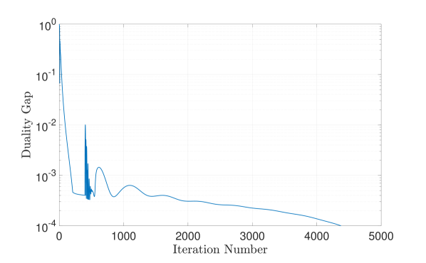
Figure 1: Duality gap during iterations in Example 1

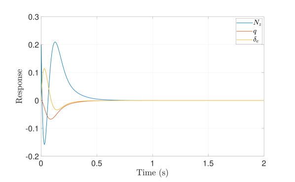
Figure 2: System response in Example 1

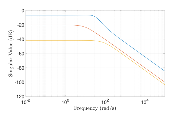
Figure 3: Singular value diagram in Example 1

Example 2.

Consider $x=\begin{bmatrix}x_{1}&x_{2}\end{bmatrix}^{T}$ and a linear system

$$\dot{{x}} =A{x}+B_{2}u+B_{1}w$$

$$z =Cx+Du$$

$$u =-Kx,$$

where

$$A=\begin{bmatrix}0.2229&0.5637\\ 0.8708&0.9984\end{bmatrix},\,B_{2}=\begin{bmatrix}0.5254&0.6644\\ 0.3872&0.9145\end{bmatrix},$$

$$B_{1}=\begin{bmatrix}1&0\\ 0&1\end{bmatrix},\,C=\begin{bmatrix}1&0\\ 0&1\\ 0&0\\ 0&0\end{bmatrix},\,D=\begin{bmatrix}0&0\\ 0&0\\ 1&0\\ 0&1\end{bmatrix}.$$

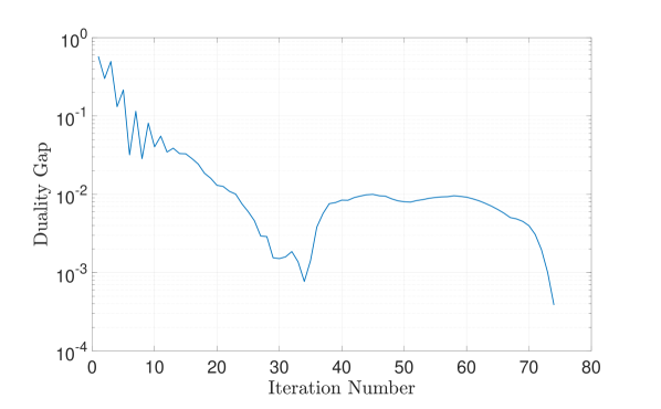
Figure 4: Duality gap during iterations in Example 2

Since all the parameters in $A$ and $B_{2}$ are uncertain with a variation of $\pm$20%, a total of $2^{8}=256$ extreme systems need to be considered in the optimization. We performed 5 trials and recorded the total computation time with our approach, where the computation time is 5.3343 s, 5.6423 s, 5.1526 s, 5.8462 s, and 5.3149 s in these trials. In this case, the average computation time is 5.4581 s. Moreover, the change of the duality gap is shown in Fig. 4. At optimality, the following results are obtained, where

$$W^{*} = \begin{bmatrix}0.1608&0.0058&0.1673&0.0665\\ 0.0058&0.0129&0.0327&0.0744\\ 0.1673&0.0327&0.6892&0.2970\\ 0.0665&0.0744&0.2970&1.2701\end{bmatrix},$$

$$\mu^{*} = 0.0410,$$

$$K^{*} = \begin{bmatrix}0.9643&2.1060\\ 0.2088&5.6843\end{bmatrix},$$

$$\gamma^{*} = 4.9411.$$

In the simulation, $w$ is considered as a vector of the impulse disturbance. For illustration purposes, the simulation considers the nominal system and an extreme system with all the uncertain parameters reaching their lower bounds, then the responses of all state variables are shown in Fig. 5. The dashed line shows the response of the extreme system, and the solid line indicates the response of the nominal system. It can be seen that for the extreme system, the closed-loop stability is suitably ensured despite the existence of parametric uncertainties. As clearly observed, the performance of the extreme system is slightly worse than the nominal system, but the difference of the dynamic response in terms of the extreme system and the nominal system is not significant. Hence, the robustness of the proposed approach is validated. Similarly, the singular value diagram of $H(s)$ is shown in Fig. 6, and the maximum singular value is given by 10.54 dB, which is equivalent to 3.3651 in magnitude, and it can be seen that it is bounded by $\gamma^{*}$.

Notice that the effectiveness of the proposed methodology in terms of computation can be more clearly demonstrated when there are a large number of extreme systems. Hence, a comparison study is carried out, where a well-established cutting-plane algorithm as presented in [42] is used. Note that this method has been demonstrated its effectiveness in solving a class of $\mathcal{H}_{2}$ and $\mathcal{H}_{\infty}$ problems in the parameter space. The numerical procedures are given below:

Step 1: Set $l=0$ and define the polytope $\mathscr{P}^{0}\supseteq\mathscr{C}_{U}$.

Step 2: Solve the linear programming problem: $(W^{l},\mu^{l})=\textup{argmax}\{\mu:(W,\mu)\in\mathscr{P}^{l}\}$.

Step 3: If $(W^{l},\mu^{l})\in\mathscr{C}_{U}$, $(W^{l},\mu^{l})$ is the optimal solution. Otherwise, generate a separating hyperplane and define $\mathscr{P}^{l+1}$. Set $l\leftarrow l+1$ and return to Step 2.

Essentially in the approach presented in [42], a suitable polytope $\mathscr{P}^{0}$ is initialized such that $\mathscr{C}_{U}$ is a subset of $\mathscr{P}^{0}$. Then, the associated linear constraint is solved in the linear programming routine (which is conducted within the polytope). For invoked nonlinear constraints, the cutting plane technique (also known as the outer linearization method) is adopted, where the satisfaction/violation condition of the nonlinear constraints is checked. If they are violated, half space (i.e., the cutting plane) will be generated and constructed for separation and update of the polytope in an iterative framework. Subsequently, the cutting planes are implemented as linear inequality constraints in the linear programming routine. In fact, this method makes an appropriate estimation of an unknown nonlinear set by iteratively involving a series of linear constraints without leading to infeasibility. However, with such a large number of extreme systems, the optimization process is unfortunately terminated with unsuccessful outcomes. The reason is that, in each iteration, a number of cutting planes could be generated and incorporated into the new linear programming routine, and these definitely lead to huge amount of computational efforts to solve this optimization problem.

Additionally, some existing numerical solvers, such as Gurobi [49] and SCS [50], are not capable to solve this optimization problem. However, with an ADMM framework in our proposed development, the original optimization problem is decomposed into a series of manageable sub-problems that can be solved effectively. This is because that, in each iteration, the explicit solution to these sub-problems can be obtained very efficiently. In this case, our proposed approach alleviates the computational burden with the splitting scheme.

Furthermore, the LQR controller is used as a benchmark for comparison of the system performance. Note that for the LQR controller, it is determined by the algebraic Riccati equation. Then, the extreme system is used again in the comparison, and the system response is presented in Fig. 7, where the dashed line represents the response with the proposed controller and the solid line indicates the response with the LQR controller. It is pertinent to note that for the purpose of a fair comparison, weighting matrices in the LQR are tuned such that the control inputs are at the same level as those attained in our proposed method. Essentially our proposed method demonstrates superior performance over the LQR approach, which can be clearly observed from Fig. 7. This is because parametric uncertainties are considered in our proposed method, and the disturbance attenuation is suppressed at its minimal level; however, the LQR does not take parametric uncertainties and disturbance attenuation into consideration.

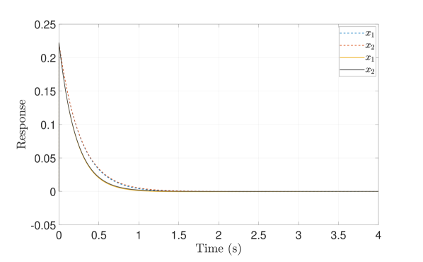
Figure 5: System response in Example 2 (dashed line: extreme system; solid line: nominal system)

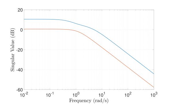
Figure 6: Singular value diagram in Example 2

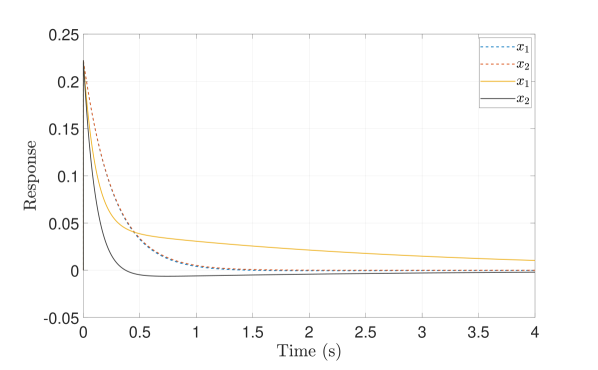
Figure 7: System response in Example 2 (dashed line: the proposed method; solid line: the LQR method)

V Conclusion

In this work, the symmetric Gauss-Seidel ADMM algorithm is presented to solve the $\mathcal{H}_{\infty}$ guaranteed cost control problem, and the development and formulation of numerical procedures is given in detail (with invoking a suitably interesting problem re-formulation based on the Schur complement). Through a parameterization technique (where the stabilizing controllers are characterized by an appropriate convex parameterization which is described and established analytically in our work here), the robust stability and performance can be suitably achieved in the presence of parametric uncertainties. An upper bound of all feasible $\mathcal{H}_{\infty}$ performances is minimized over the uncertain domain, and the minimum disturbance attenuation level is obtained through the optimization. Furthermore, the algorithm is evaluated based on two suitably appropriate illustrative examples, and the simulation results successfully reveal the practical appeal of the proposed methodology in terms of computation, and also clearly validate the results on robust stability and performance. This work can be further extended to the mixed $\mathcal{H}_{2}$/$\mathcal{H}_{\infty}$ control problem, which aims to balance the trade-off between performance and robustness. Particularly, given an prescribed $\mathcal{H}_{\infty}$ attenuation level, the objective is to seek the optimal $\mathcal{H}_{2}$ control gain, where the nominal performance index is minimized with the imposed pertinent constraints.

References

- [1] X. Kai, C. Wei, and L. Liu, “Robust extended Kalman filtering for nonlinear systems with stochastic uncertainties,” IEEE Transactions on Systems, Man, and Cybernetics-Part A: Systems and Humans, vol. 40, no. 2, pp. 399–405, 2009.
- [2] D. Wang, D. Liu, H. Li, B. Luo, and H. Ma, “An approximate optimal control approach for robust stabilization of a class of discrete-time nonlinear systems with uncertainties,” IEEE Transactions on Systems, Man, and Cybernetics: Systems, vol. 46, no. 5, pp. 713–717, 2016.
- [3] Q. Zhu and H. Wang, “Output feedback stabilization of stochastic feedforward systems with unknown control coefficients and unknown output function,” Automatica, vol. 87, pp. 166–175, 2018.
- [4] H. Wang and Q. Zhu, “Global stabilization of a class of stochastic nonlinear time-delay systems with SISS inverse dynamics,” IEEE Transactions on Automatic Control, vol. 65, no. 10, pp. 4448–4455, 2020.
- [5] L. Ma, N. Xu, X. Zhao, G. Zong, and X. Huo, “Small-gain technique-based adaptive neural output-feedback fault-tolerant control of switched nonlinear systems with unmodeled dynamics,” IEEE Transactions on Systems, Man, and Cybernetics: Systems, 2020.
- [6] X. Chen, H. Zhao, S. Zhen, and H. Sun, “Novel optimal adaptive robust control for fuzzy underactuated mechanical systems: a Nash game approach,” IEEE Transactions on Fuzzy Systems, 2020.
- [7] X. Chen, H. Zhao, H. Sun, S. Zhen, and A. Al Mamun, “Optimal adaptive robust control based on cooperative game theory for a class of fuzzy underactuated mechanical systems,” IEEE Transactions on Cybernetics, 2020.
- [8] I. R. Petersen and C. V. Hollot, “A Riccati equation approach to the stabilization of uncertain linear systems,” Automatica, vol. 22, no. 4, pp. 397–411, 1986.
- [9] I. R. Petersen, “A stabilization algorithm for a class of uncertain linear systems,” Systems & Control Letters, vol. 8, no. 4, pp. 351–357, 1987.
- [10] J. Bernussou, P. L. D. Peres, and J. C. Geromel, “A linear programming oriented procedure for quadratic stabilization of uncertain systems,” Systems & Control Letters, vol. 13, no. 1, pp. 65–72, 1989.
- [11] J. C. Doyle, K. Glover, P. P. Khargonekar, and B. A. Francis, “State-space solutions to standard and control problems,” IEEE Transactions on Automatic control, vol. 34, no. 8, pp. 831–847, 1989.
- [12] L. Xie and E. de Souza Carlos, “Robust control for linear systems with norm-bounded time-varying uncertainty,” IEEE Transactions on Automatic Control, vol. 37, no. 8, pp. 1188–1191, 1992.
- [13] K. Zhou and P. P. Khargonekar, “An algebraic Riccati equation approach to optimization,” Systems & Control Letters, vol. 11, no. 2, pp. 85–91, 1988.
- [14] X.-H. Chang and Y. Liu, “Robust filtering for vehicle sideslip angle with quantization and data dropouts,” IEEE Transactions on Vehicular Technology, vol. 69, no. 10, pp. 10 435–10 445, 2020.
- [15] B. Wu, X.-H. Chang, and X. Zhao, “Fuzzy output feedback control for nonlinear NCSs with quantization and stochastic communication protocol,” IEEE Transactions on Fuzzy Systems, 2020.
- [16] C. Scherer, “-control by state feedback: An iterative algorithm and characterization of high-gain occurence,” Systems & Control letters, vol. 12, no. 5, pp. 383–391, 1989.
- [17] Y. Qi, Y. Liu, and B. Niu, “Event-triggered filtering for networked switched systems with packet disorders,” IEEE Transactions on Systems, Man, and Cybernetics: Systems, 2019.
- [18] Y. Qi, X. Zhao, and J. Huang, “ filtering for switched systems subject to stochastic cyber attacks: A double adaptive storage event-triggering communication,” Applied Mathematics and Computation, vol. 394, p. 125789, 2021.
- [19] X. Qi, M. V. Salapaka, P. G. Voulgaris, and M. Khammash, “Structured optimal and robust control with multiple criteria: A convex solution,” IEEE Transactions on Automatic Control, vol. 49, no. 10, pp. 1623–1640, 2004.
- [20] L. Furieri, Y. Zheng, A. Papachristodoulou, and M. Kamgarpour, “An input-output parametrization of stabilizing controllers: amidst Youla and system level synthesis,” IEEE Control Systems Letters, vol. 3, no. 4, pp. 1014–1019, 2019.
- [21] W. Lin and E. Bitar, “A convex information relaxation for constrained decentralized control design problems,” IEEE Transactions on Automatic Control, vol. 64, no. 11, pp. 4788–4795, 2019.
- [22] J. Ma, H. Zhu, M. Tomizuka, and T. H. Lee, “On robust stability and performance with a fixed-order controller design for uncertain systems,” IEEE Transactions on Systems Man Cybernetics: Systems, 2021.
- [23] J. Ma, H. Zhu, X. Li, C. W. de Silva, and T. H. Lee, “Robust fixed-order controller design with common Lyapunov strictly positive realness characterization,” arXiv preprint arXiv:2006.03462, 2020.
- [24] J. C. Geromel, P. L. D. Peres, and J. Bernussou, “On a convex parameter space method for linear control design of uncertain systems,” SIAM Journal on Control and Optimization, vol. 29, no. 2, pp. 381–402, 1991.
- [25] D. P. Bertsekas and H. Yu, “A unifying polyhedral approximation framework for convex optimization,” SIAM Journal on Optimization, vol. 21, no. 1, pp. 333–360, 2011.
- [26] K. Puttannaiah, J. A. Echols, and A. A. Rodriguez, “A generalized control design framework for stable multivariable plants subject to simultaneous output and input loop breaking specifications,” in 2015 American Control Conference (ACC). IEEE, 2015, pp. 3310–3315.
- [27] K. Puttannaiah, A. A. Rodriguez, K. Mondal, J. A. Echols, and D. G. Cartagena, “A generalized mixed-sensitivity convex approach to hierarchical multivariable inner-outer loop control design subject to simultaneous input and output loop breaking specifications,” in 2016 American Control Conference (ACC). IEEE, 2016, pp. 5632–5637.
- [28] C. Bergeling, R. Pates, and A. Rantzer, “H-infinity optimal control for systems with a bottleneck frequency,” IEEE Transactions on Automatic Control, vol. 66, no. 6, pp. 2732–2738, 2020.
- [29] Y. Zheng, S. E. Li, K. Li, and W. Ren, “Platooning of connected vehicles with undirected topologies: Robustness analysis and distributed controller synthesis,” IEEE Transactions on Intelligent Transportation Systems, vol. 19, no. 5, pp. 1353–1364, 2017.
- [30] S. Boyd, N. Parikh, E. Chu, B. Peleato, and J. Eckstein, “Distributed optimization and statistical learning via the alternating direction method of multipliers,” Foundations and Trends in Machine Learning, vol. 3, no. 1, pp. 1–122, 2011.
- [31] D. Sun, K.-C. Toh, and L. Yang, “A convergent 3-block semiproximal alternating direction method of multipliers for conic programming with 4-type constraints,” SIAM Journal on Optimization, vol. 25, no. 2, pp. 882–915, 2015.
- [32] A. Makhdoumi and A. Ozdaglar, “Convergence rate of distributed ADMM over networks,” IEEE Transactions on Automatic Control, vol. 62, no. 10, pp. 5082–5095, 2017.
- [33] D. Du, X. Li, W. Li, R. Chen, M. Fei, and L. Wu, “ADMM-based distributed state estimation of smart grid under data deception and denial of service attacks,” IEEE Transactions on Systems, Man, and Cybernetics: Systems, vol. 49, no. 8, pp. 1698–1711, 2019.
- [34] B. Chen, D. W. Ho, W.-A. Zhang, and L. Yu, “Distributed dimensionality reduction fusion estimation for cyber-physical systems under dos attacks,” IEEE Transactions on Systems, Man, and Cybernetics: Systems, vol. 49, no. 2, pp. 455–468, 2017.
- [35] Z. Wu, Z. Li, Z. Ding, and Z. Li, “Distributed continuous-time optimization with scalable adaptive event-based mechanisms,” IEEE Transactions on Systems, Man, and Cybernetics: Systems, vol. 50, no. 9, pp. 3252–3257, 2020.
- [36] B. Wei and F. Xiao, “Distributed consensus control of linear multiagent systems with adaptive nonlinear couplings,” IEEE Transactions on Systems, Man, and Cybernetics: Systems, 2019.
- [37] C. Peng, J. Zhang, and Q.-L. Han, “Consensus of multiagent systems with nonlinear dynamics using an integrated sampled-data-based event-triggered communication scheme,” IEEE Transactions on Systems, Man, and Cybernetics: Systems, vol. 49, no. 3, pp. 589–599, 2018.
- [38] C. Yang, T. Huang, A. Zhang, J. Qiu, J. Cao, and F. E. Alsaadi, “Output consensus of multiagent systems based on PDEs with input constraint: A boundary control approach,” IEEE Transactions on Systems, Man, and Cybernetics: Systems, 2018.
- [39] C. Chen, B. He, Y. Ye, and X. Yuan, “The direct extension of ADMM for multi-block convex minimization problems is not necessarily convergent,” Mathematical Programming, vol. 155, no. 1-2, pp. 57–79, 2016.
- [40] A. A. Adegbege and Z. E. Nelson, “A Gauss-Seidel type solver for the fast computation of input-constrained control systems,” Systems & Control Letters, vol. 97, pp. 132–138, 2016.
- [41] L. Chen, D. Sun, and K.-C. Toh, “An efficient inexact symmetric Gauss-Seidel based majorized ADMM for high-dimensional convex composite conic programming,” Mathematical Programming, vol. 161, no. 1-2, pp. 237–270, 2017.
- [42] P. L. D. Peres, J. C. Geromel, and S. R. Souza, “Optimal state feedback control for continuous-time linear systems,” Journal of Optimization Theory and Applications, vol. 82, no. 2, pp. 343–359, 1994.
- [43] J. Ma, Z. Cheng, X. Zhang, M. Tomizuka, and T. H. Lee, “Optimal decentralized control for uncertain systems by symmetric Gauss–Seidel semi-proximal ALM,” IEEE Transactions on Automatic Control, vol. 66, no. 11, pp. 5554–5560, 2021.
- [44] J. Ma, Z. Cheng, H. Zhu, X. Li, M. Tomizuka, and T. H. Lee, “Convex parameterization and optimization for robust tracking of a magnetically levitated planar positioning system,” IEEE Transactions on Industrial Electronics, vol. 69, no. 4, pp. 3798–3809, 2021.
- [45] D. P. Bertsekas and J. N. Tsitsiklis, Parallel and Distributed Computation: Numerical Methods. Upper Saddle River, NJ: Prentice-Hall, 1989.
- [46] J. Ma, S.-L. Chen, C. S. Teo, A. Tay, A. Al Mamun, and K. K. Tan, “Parameter space optimization towards integrated mechatronic design for uncertain systems with generalized feedback constraints,” Automatica, vol. 105, pp. 149–158, 2019.
- [47] J. C. Geromel, P. L. D. Peres, and S. R. Souza, “Convex analysis of output feedback structural constraints,” in Proceedings of the 32nd IEEE Conference on Decision and Control, 1993, pp. 1363–1364.
- [48] I. R. Petersen, “A procedure for simultaneously stabilizing a collection of single input linear systems using non-linear state feedback control,” Automatica, vol. 23, no. 1, pp. 33–40, 1987.
- [49] Gurobi Optimization, LLC, “Gurobi Optimizer Reference Manual,” 2021. [Online]. Available: https://www.gurobi.com
- [50] O. Brendan, C. Eric, P. Neal, and B. Stephen, “Operator splitting for conic optimization via homogeneous self-dual embedding,” Journal of Optimization Theory and Applications, vol. 169, no. 3, pp. 1042–1068, 2016.