Creation and Evolution of Impact-generated Reduced Atmospheres of Early Earth

Abstract

The origin of life on Earth seems to demand a highly reduced early atmosphere, rich in CH₄, H₂, and NH₃, but geological evidence suggests that Earth’s mantle has always been relatively oxidized and its emissions dominated by CO₂, H₂O, and N₂. The paradox can be resolved by exploiting the reducing power inherent in the “late veneer,” i.e., material accreted by Earth after the Moon-forming impact. Isotopic evidence indicates that the late veneer consisted of extremely dry, highly reduced inner solar system materials, suggesting that Earth’s oceans were already present when the late veneer came. The major primary product of reaction between the late veneer’s iron and Earth’s water was H₂. Ocean vaporizing impacts generate high pressures and long cooling times that favor CH₄ and NH₃. Impacts too small to vaporize the oceans are much less productive of CH₄ and NH₃, unless (i) catalysts were available to speed their formation, or (ii) additional reducing power was extracted from pre-existing crustal or mantle materials. The transient H₂-CH₄ atmospheres evolve photochemically to generate nitrogenated hydrocarbons at rates determined by solar radiation and hydrogen escape, on timescales ranging up to tens of millions of years and with cumulative organic production ranging up to half a kilometer. Roughly one ocean of hydrogen escapes. The atmosphere after the methane’s gone is typically H₂ and CO rich, with eventual oxidation to CO₂ rate-limited by water photolysis and hydrogen escape.

1 Introduction

The modern science of the origin of life on Earth begins with Haldane (1929) and Oparin (1938). Both argued that a highly reduced early terrestrial environment — profoundly unlike the world of today, even with O₂ removed — was needed. Oparin’s specific emphasis on methane, ammonia, formaldehyde, and hydrogen cyanide as primordial materials suitable for further development remains a recurring theme in origin of life studies (Urey, 1952; Oró and Kamat, 1961; Ferris et al., 1978; Stribling and Miller, 1987; Oró et al., 1990; Ricardo et al., 2004; Powner et al., 2009; Sutherland, 2016; Benner et al., 2019a). Although some of these materials — formaldehyde in particular — can be generated under weakly reducing conditions (Pinto et al., 1980; Benner et al., 2019b), others (such as cyanamide and cyanoacetylene) require strongly reducing conditions. The hypothesized reducing atmosphere inspired the famous and often-replicated Miller-Urey experiments, in which sparked or UV irradiated gas mixtures spontaneously generate a wide range of organic molecules (Miller, 1953, 1955; Miller and Urey, 1959; Cleaves et al., 2008; Johnson et al., 2008).

The geological argument against a reducing early atmosphere is nearly as old (e.g., Poole, 1951), although often accompanied by the caveat that things could have been different before the rock record (e.g., Holland, 1964; Abelson, 1966; Walker, 1977; Holland, 1984). The underlying presumption is that the atmosphere should have resembled volcanic gases. Modern volcanic gases are roughly consistent with the QFM (quartz-fayalite-magnetite) mineral buffer, for which the redox state is determined by chemical reactions between ferrous (Fe⁺²) and ferric iron (Fe⁺³). At typical magma temperatures, QFM predicts that H₂ and CO would be present at percent levels compared to H₂O and CO₂, and that methane and ammonia would be negligible.

Some studies suggest that the Archean mantle had a similar redox state to today (Delano, 2001; Canil, 2002; Rollinson et al., 2017), while rare earth elements in zircons suggest a Hadean mantle consistent with QFM (Trail et al., 2012). Large uncertainties in observationally derived oxygen fugacities ($\pm 2$ in $\log_{10}\!{\left(f_{\mathrm{O}_{2}}\right)}$) may obscure a secular trend, while some simplifying assumptions made in earlier $f_{\mathrm{O}_{2}}$ studies are open to question (Wang et al., 2019). (The redox state of rocks is usually described by oxygen fugacity $f_{\mathrm{O}_{2}}$, which describes the formal abundance of O₂ gas in units of atmospheres.) Two recent studies that use filtered samples hint that $\log_{10}\!{\left(f_{\mathrm{O}_{2}}\right)}$ of the mantle increased by $\sim\!1.3$ from the early Archean to Proterozoic (Aulbach and Stagno, 2016; Nicklas et al., 2019).

Concurrently, a body of experimental evidence has accumulated suggesting that ferrous silicates in Earth’s mantle disproportionate under great pressure into ferric iron and metallic iron, with the latter expected to migrate to the core (Frost and McCammon, 2008). This would leave the mantle, or at least part of the mantle, in a QFM-like state of oxidation from the time our planet first became big enough to be called Earth (Armstrong et al., 2019).

Given the incompatibility of a QFM mantle with a reduced atmosphere, workers have turned to impact degassing, in which gases are directly released into the atmosphere on impact (Matsui and Abe, 1986; Tyburczy et al., 1986). Most impactors are much more reduced than the mantle and often better endowed (gram per gram) in atmophile elements (Urey, 1952; Schaefer and Fegley, 2007; Hashimoto et al., 2007; Sugita and Schultz, 2009). Many meteorites, including ordinary chondrites and enstatite chondrites, contain substantial amounts of metallic iron and iron sulfides. Gases that equilibrate with these highly reduced meteoritic materials would be highly reduced themselves (Kasting, 1990; Schaefer and Fegley, 2007; Hashimoto et al., 2007; Schaefer and Fegley, 2010; Kuwahara and Sugita, 2015; Schaefer and Fegley, 2017), provided that there is enough iron to reduce all the atmophiles in the impactor. But if there are more atmophiles to reduce than iron to reduce them, the gas composition can evolve to a much more oxidized state (Schaefer and Fegley, 2017).

Several of the new impact-degassing studies (Hashimoto et al., 2007; Schaefer and Fegley, 2007, 2010, 2017) calculate gas compositions in equilibrium with mineral assemblages at fixed pressures, with temperature treated as an independent variable. These calculations often promise big yields of CH₄ and NH₃ at low temperatures. However, actual yields depend on the quench conditions in the gas as it cools after the impact. A cooling gas is said to have quenched when the chemical reactions maintaining equilibrium between species become so sluggish that the composition of the gas freezes (Zel’dovich and Raizer, 1967). Quenching is mostly determined by temperature. Gas phase reactions for making CH₄ from CO are strongly inhibited by low temperatures, and those for making NH₃ from N₂ are even more strongly inhibited, so unless an abundant catalyst were available to lower the effective quench temperature (Kress and McKay, 2004), there is a tendency for the shock-heated gas to quench to CO, N₂, and H₂. Of the new studies, only Kuwahara and Sugita (2015) have attempted to calculate quench conditions, but their results are problematic because they used the entropy of shocked silica to estimate the entropy of shocked carbonaceous chondrites, which results in artificially low temperatures and artificially large amounts of methane. Finally, in a full account, the quenched plume of impact gases would be mixed into, and diluted by, the pre-existing atmosphere.

This study follows the lead of Genda et al. (2017a, b) and Benner et al. (2019a) in addressing how the largest cosmic impacts changed the ocean and atmosphere that were already present on Earth. We go beyond Genda et al. (2017a, b) and Benner et al. (2019a) in addressing not just the single largest impact but also a full range of sizes, extending to impacts 100 and even 1000 times smaller (Hadean Earth would have experienced scores of these). Our particular focus is on impacts that process the entire atmosphere and hydrosphere. This differs from previous studies of smaller impacts that find that the main product of impact is HCN, and this only in atmospheres with C/O ratios greater than unity (cf., Chyba and Sagan, 1992; Fegley and Prinn, 1998). Section 2 provides a brief summary of impacts after the Moon formed as constrained by geochemistry and the craters of the Moon. Section 3 addresses impact-generation of methane-rich atmospheres on Earth. The emphasis is on impacts that are big enough to vaporize the oceans, as these produce long-lasting hot conditions at high pressures, and thus can be highly favorable to methane and sometimes even to ammonia. Section 4 uses a simple model to address the subsequent photochemical evolution of these atmospheres. The emphasis here is on the fate of methane and the production of organic material and hazes, on the photochemistry of nitrogen and the generation of HCN and other nitrogenated organics, and on hydrogen escape. Ammonia is (mostly) deferred to the Discussion.

2 The Late Veneer

The highly siderophile elements (HSEs) comprise seven heavy metals (Ru, Rh, Pd, Os, Ir, Pt, and Au) with very strong tendencies to partition into planetary cores. If Earth’s mantle and core were fully equilibrated almost all of its HSEs would be in the core, and the tiny remnant in the mantle would be highly chemically fractionated (Walker, 2009; Day et al., 2016; Rubie et al., 2015, 2016). But this is not what is seen. Rather, the mantle contains a modest cohort of excess HSEs that, to first approximation, are present in roughly the same relative abundances that they have in chondritic meteorites (Day et al., 2016). One explanation is that the excess HSEs were dropped into the mantle and left stranded there some time after core formation was complete. If the mantle’s HSEs were added with other elements in chondritic proportions, they correspond to about 0.5% of Earth’s mass (Anders, 1989). The late-added mass carrying the HSEs is usually called the “late veneer.”

The late veneer measured in this way is very big. Viewed literally, 0.5% of Earth’s mass corresponds to a veneer 20 km thick. Gathered into a sphere, it corresponds to a rocky world 2300 km diameter — as big as Pluto, and more massive. We will call this the “maximum HSE” veneer. If the veneer were sourced from fragments of differentiated worlds, the veneer mass could be a little smaller or much bigger.

Historically, the late veneer was presumed volatile-rich, as would be expected if the last materials to fall to Earth fell from the cold distant outer solar system (Anders and Owen, 1977; Wänke and Dreibus, 1988; Dreibus and Wänke, 1989; Albarède et al., 2013). However, the late veneer now appears constrained by Ru isotopes to resemble either enstatite chondrites, enstatite achondrites (aka aubrites), or iron meteorites of type IAB, and thus appears to come from the same deep inner solar system reservoir as Earth itself (Dauphas, 2017; Fischer-Gödde and Kleine, 2017; Bermingham et al., 2018; Hopp and Kleine, 2018). All of our samples of these materials are profoundly reduced and very dry. This apparently excludes the late veneer as the source of water on Earth (Fischer-Gödde and Kleine, 2017), and thus the late veneer can be presumed to have impacted into an Earth already fully plenished with oceans, a view also consistent with oxygen isotopes (Greenwood et al., 2018). The late veneer’s role changes from water bearer to water changer: it must now be viewed as a source of reducing power injected into Earth’s near-surface environment (Genda et al., 2017a, b; Benner et al., 2019a).

The total reducing power delivered by the maximum late veneer can be illustrated by using all of its metallic iron to reduce water to hydrogen, in stoichiometry $\mathrm{Fe}+\mathrm{H}_{2}\mathrm{O}\rightarrow\mathrm{FeO}+\mathrm{H}_{2}$. The iron that accompanied the mantle’s excess HSEs corresponded to $1\times 10^{25}$ g of metal. Because the HSEs remained in the mantle neither they nor the iron that came with them went to the core, and thus we can be confident that the iron was oxidized at the surface, in the crust, or in the mantle. There is enough iron in the late veneer to reduce $1.8\times 10^{23}$ moles of H₂O to H₂ and FeO, which corresponds to reducing of 2.3 oceans of water to hydrogen.

If the late veneer were characterized by size-number statistics typical of stray solar system bodies, it is likely that most of the mantle’s HSE excess was carried by a single Pluto-sized body (Sleep et al., 1989; Tremaine and Dones, 1993; Bottke et al., 2010; Brasser et al., 2016; Genda et al., 2017a). Comparison with the uncertain but apparently much smaller lunar HSE excess (Day et al., 2016) is consistent with the conjecture that the maximum HSE event was singular (Brasser et al., 2016; Morbidelli et al., 2018), although this is not required, as there are other ways of explaining the scarcity of lunar HSEs that do not imply different accretion rates for Earth and Moon (cf., Kraus et al., 2015).

But even if the late veneer were delivered by one body, it does not follow that its mass was added to Earth in a moment. There is a considerable likelihood, estimated as 50% by Agnor and Asphaug (2004), that an impact results not in a merger but rather in the disintegration of the smaller body. The debris are distributed in a ring around the Sun coincident with Earth’s orbit and swept up by Earth over tens or hundreds of thousands of years (Genda et al., 2017a, b). Few of the debris are swept up by the Moon, owing to the much greater gravitational cross-section of Earth with respect to debris in quasi-circular orbits (Genda et al., 2017a). This kind of distributed event is likely to strand nearly all of its HSEs in the crust or at shallow depths in Earth’s mantle, while the direct impact of a Pluto-sized body might be expected to drive much of the impactor’s core directly into our own. Stranding all the newly added HSEs in the mantle without fractionation fulfills a second independent requirement imposed by the mantle’s Ru isotopes, which were not mass-fractionated by partitioning between the mantle and core (Fischer-Gödde and Kleine, 2017; Hopp and Kleine, 2018). Dividing the impactor into myriads of smaller particles would also be more effective at chemically reducing Earth’s atmosphere and ocean. For example, Genda et al. (2017b) model a Moon-sized impactor and find that 60% of the iron would be divided into mm-size droplets. The overall picture resembles that suggested by Urey (1952), who wrote that “materials would have fallen through the atmosphere in the form of iron and silicate rains and would have reacted with the atmosphere [and hydrosphere] in the process.”

An important caveat is that a maximum HSE impact may not couple well to the oceans. A Pluto-sized impact would blanket Earth in tens of kilometers of impact ejecta, which is so much deeper than the oceans that much of the iron may have been buried before it could react with water. Under these conditions, the buried iron would have remained unoxidized in the upper mantle for a considerable period of time. We know from the presence of the HSEs and the unfractionated Ru isotopes that the iron was not removed to the core. The iron must therefore have strongly influenced the redox state of volcanic gases until its oxidation was complete. The effect of this is to prolong the influence of the maximum HSE event to geological time scales.

Table 1: Some Representative Hadean impacts

						Products, dry atmospherea [bars]
Category	Nb	$M_{i}^{c}$ [g]	Vapd	Rede	CO${}_{2}^{f}$	H2	CO	CO2	CH4	NH3
Max HSE	0-1	2(25)	200	2	100	57	5(-6)	1.4(-5)	9.0	0.08
QFIg					100	74	1(-5)	2(-6)	7.6	0.050
IWg					100	35	4(-5)	6(-4)	13.7	0.086
QFMg					100	10	0.11	65.6	13.6	0.01
Pretty Bigh	0-2	2.5(24)	20	0.2	20	7.6	5(-4)	0.06	2.9	0.03
					5	7.4	6(-6)	4(-4)	0.34	0.01
“Ceres”	1-4	1(24)	8	0.08	5	3.9	3(-4)	0.06	0.52	0.006
“Vesta”	2-10	2.5(23)	2	0.02	5	3.9	0.06	1.6	0.17	0.002
					2	2.6	6(-4)	0.4	0.054	0.0015
					1	2.0	2(-4)	0.14	0.023	0.0011
QFMi					2	1.8	1(-5)	0.02	0.28	0.06
Sub-Vesta	3-20	1(23)	0.8	0.008	5	2.7	0.005	2.7	0.008	8(-4)
QFMi					2	1.5	6(-5)	0.1	0.36	0.037
S.Pole-Ait.j	10-100	1(22)	0.1	8(-4)	2	0.37	0.008	1.5	1(-7)	2(-5)
QFMi					2	0.65	0.015	1.32	1(-6)	7(-5)
$a$ – The dry atmosphere presumes that all water has condensed at the surface.
$b$ – Number of Hadean impacts in each class, bracketed between minimum and maximum veneer
$c$ – $M_{i}$ presumes 33% metallic iron, like EH (high iron enstatite) chondrites or bulk Earth
$d$ – Oceans of water that could be vaporized by the impact
$e$ – Potential reducing power of the impact, expressed as oceans of water that can be reduced to H2
$f$ – Atmospheric CO2 before the impact [100 bars = 2300 moles cm-2]
$g$ – Assumed to equilibrate with the named mineral buffer (defined in Appendix A)
$h$ – Plausible size of biggest impact in a minimum late veneer
$i$ – Atmosphere and ocean are assumed to equilibrate with QFM buffer at 650 K
$j$ – South Pole-Aitken is the largest impact basin preserved on the Moon

There is also a small chance that the late veneer is an illusion. It has been suggested that Earth’s HSE excess may date to the Moon-forming impact itself (Newsom and Taylor, 1989; Sleep, 2016; Brasser et al., 2016). If so, the mantle’s HSE excess overestimates the amount of reducing power delivered to Earth after the Moon-forming impact. A crude lower bound on the late veneer can be extrapolated from the lunar crater record (Sleep et al., 1989; Zahnle and Sleep, 1997, 2006). This scaling suggests that the “minimum late veneer” delivered between 3-30% of the mass as the maximum HSE veneer. The large uncertainty, and large total mass striking Earth compared to the Moon, both arise from the high probability that all the largest bodies in a given population hit the Earth (Sleep et al., 1989).

Table 1 lists a representative sampling of maximum and minimum late veneer impacts. The number of bodies in any given size class is estimated from the cumulative relation $N(>\!m)\propto m^{-b}$, with $0.5\!<\!b\!<\!0.9$, with the smaller number based on the number of lunar basins and with the larger number based on the total cumulative mass of the maximum late veneer using methods described by Zahnle and Sleep (1997). The number of oceans that can be vaporized assumes that 50% of the impact energy is available to evaporate an ocean ($1.4\times 10^{24}$g) of water and heat the steam to 1500 K. The number of oceans that can be reduced to H₂ assumes an EH enstatite chondritic composition with 33% Fe by mass and that the reaction $\mathrm{Fe}+\mathrm{H}_{2}\mathrm{O}\rightarrow\mathrm{FeO}+\mathrm{H}_{2}$ goes to completion. Other entries in Table 1 are discussed as they arise.

Evidence has recently emerged that Earth’s molybdenum — another siderophile element, but somewhat less so than the HSEs — has an isotopic composition distinct from Earth’s HSEs (Budde et al., 2019). This has been interpreted by its discoverers to mean that Theia — the name widely given to the Moon-forming impactor — was made of different stuff than the late veneer (Budde et al., 2019). Budde et al. (2019) even suggest that Theia was the source of Earth’s water, although in our opinion it seems equally plausible that Earth’s distinctive Mo predates the Moon-forming impact. From our perspective here it makes little difference whether Earth’s water was delivered by Theia or predated Theia, because in either case the water was present on Earth when the late veneer came.

3 Thermochemical Model

The redox state of gases in equilibrium with rocks is often described by mineral buffers that govern the capacity of the rock to consume or release oxygen. Three such buffers are described in Appendix A. Mineral buffering is most likely to matter when the rock-to-atmophile ratio is large, as it is in meteorites or for Earth-like planets considered as a whole. Mineral buffers are less obviously appropriate for describing the interaction of meteorites with oceans and atmospheres that are much bigger than the meteorite (Elkins-Tanton and Seager, 2008). Only the very biggest post-Moon-forming impacts are big enough for a mineral buffer set by the impactor to apply on a global scale. For anything smaller, the oxygen in the atmosphere and ocean much exceeds the reducing power in the impactor, and hence the reduced mineral buffers are exhausted before the atmosphere and ocean can fully equilibrate (Elkins-Tanton and Seager, 2008; Schaefer and Fegley, 2017). What this means is that, in most cases, a better approximation than hewing to a mineral buffer is to stoichiometrically remove the oxygen scavenged by metallic iron from the atmosphere and ocean, and then compute the resulting equilibria amongst the gases.

3.1 Equilibrium chemistry

We solve for five potentially major gases — H₂, H₂O, CO, CO₂, and CH₄ — while presuming that other gases are minor. In particular, we treat nitrogen as a minor perturbation, and we ignore sulfur and chlorine. We treat the equilibrium chemistry of the atmosphere as a whole. We solve for the column number densities $N_{j}$ and for the partial pressures $p_{j}$ of the 5 species. The total pressure $p$ is the weight of the atmosphere,

$$p=g\sum_{j}N_{j}m_{j},$$ (1)

where $g$ is the gravity and $m_{j}$ is the mass of species $j$. Partial pressures $p_{j}$ are related to column densities and the total pressure by

$$p_{j}={pN_{j}\over\sum_{j}N_{j}}.$$ (2)

Note that, in general, $p_{j}\neq N_{j}m_{j}g$; i.e., partial pressures are proportional to number fractions, not mass fractions.

In the five gas system, hydrogen and carbon are conserved:

$$N_{\mathrm{H}}=2N_{\mathrm{H}_{2}}+2N_{\mathrm{H}_{2}\mathrm{O}}+4N_{\mathrm{CH}_{4}}$$ (3)

and

$$N_{\mathrm{C}}=N_{\mathrm{CO}}+N_{\mathrm{CO}_{2}}+N_{\mathrm{CH}_{4}}.$$ (4)

In the absence of a mineral buffer, oxygen is also conserved,

$$N_{\mathrm{O}}=N_{\mathrm{H}_{2}\mathrm{O}}+N_{\mathrm{CO}}+2N_{\mathrm{CO}_{2}}.$$ (5)

The other two relations needed to close the system are chemical equilibria. We use the water gas shift reaction

$${\rm CO}+{\rm H}_{2}{\rm O}\leftrightarrow{\rm CO}_{2}+{\rm H}_{2},$$ (R1)

which has equilibrium constant

$$K_{\ref{shift}}=\frac{p_{\mathrm{H}_{2}\mathrm{O}}\,p_{\mathrm{CO}}}{p_{\mathrm{H}_{2}}\,p_{\mathrm{CO}_{2}}}\approx 18.28\exp{\left(-2375.6/T-5.69\times 10^{5}/T\right)},$$ (6)

and the corresponding reaction for methane,

$${\rm CO}+3{\rm H}_{2}\leftrightarrow{\rm CH}_{4}+{\rm H}_{2}{\rm O},$$ (R2)

which has equilibrium constant

$$K_{\ref{methane}}=\frac{p_{\mathrm{CH}_{4}}\,p_{\mathrm{H}_{2}\mathrm{O}}}{p_{\mathrm{CO}}\,p^{3}_{\mathrm{H}_{2}}}\approx 5.239\times 10^{-14}\exp{\left(27285/T\right)}\;\;\mathrm{atm}^{-2}.$$ (7)

As is customary, partial pressures in Equations 6 and 7 are in atmospheres. Equilibrium constants given here are low order curve fits (Zahnle and Marley, 2014) generated using thermochemical data from Chase (1998).

When oxygen is controlled by a mineral buffer, oxygen is not conserved and a third chemical equilibrium reaction is needed to link the system to the mineral buffer. The mineral buffer supplies the oxygen fugacity $f_{\mathrm{O}_{2}}$, which has units of pressure. We use

$$2{\rm H}_{2}{\rm O}\leftrightarrow{\rm O}_{2}+2{\rm H}_{2},$$ (R3)

with equilibrium constant

$$K_{\ref{oxygen}}=\frac{p^{2}_{\mathrm{H}_{2}\mathrm{O}}}{p^{2}_{\mathrm{H}_{2}}\,f_{\mathrm{O}_{2}}}\approx 1.158\times 10^{-6}\exp{\left(59911/T\right)}\;\;\mathrm{atm}^{-1}.$$ (8)

We will suppose that the gas remains equilibrated with the mineral buffer until the metallic iron is either exhausted or physically removed from interaction with the gas. This fixes the total oxygen content of the atmosphere. Thereafter the gas phase chemistry continues to evolve with oxygen conserved in response to further cooling until the gas phase reactions themselves quench.

It is convenient to treat nitrogen species as minor perturbations, solved separately for fixed amounts of the five important CHO species. Separating N also facilitates taking into account that nitrogen species quench at higher temperatures than H, C, and O. This simplification is accurate provided that NH₃ is not a major gas. Nitrogen is conserved,

$$N_{\mathrm{N}}=N_{\mathrm{NH}_{3}}+N_{\mathrm{HCN}}+2N_{\mathrm{N}_{2}}.$$ (9)

Two chemical equilibria are needed, one for ammonia

$${\rm N}_{2}+3{\rm H}_{2}\leftrightarrow 2{\rm NH}_{3},$$ (R4)

with equilibrium constant

$$K_{\ref{ammonia}}=\frac{p^{2}_{\mathrm{NH}_{3}}}{p_{\mathrm{N}_{2}}\,p^{3}_{\mathrm{H}_{2}}}\approx 5.90\times 10^{-13}\exp{\left(13207/T\right)}\;\;\mathrm{atm}^{-2},$$ (10)

and another for HCN,

$${\rm H}_{2}{\rm O}+{\rm HCN}\leftrightarrow{\rm CO}+{\rm NH}_{3},$$ (R5)

with equilibrium constant

$$K_{\ref{HCN}}=\frac{p_{\mathrm{H}_{2}\mathrm{O}}\,p_{\mathrm{HCN}}}{p_{\mathrm{CO}}\,p_{\mathrm{NH}_{3}}}\approx 1.99\exp{\left(-6339.4/T\right)}.$$ (11)

Equations 10 and 11 reduce to a quadratic equation for NH₃. In practice HCN is never produced abundantly by shock heating in the large impacts and H₂O-CO₂ atmospheres considered in this study. The chief source of HCN in this study is photochemical, discussed in Section 4 below.

3.2 Quenching

Chemical reactions are generally fast at high temperatures and chemical equilibria are quickly established between major species. As the gas cools, chemical reactions between the more stable molecules slow down until for all practical purposes they stop and the gas composition is said to have quenched or frozen (Zel’dovich and Raizer, 1967). Here we ignore possible catalysts and address only gas phase chemistry, which is the most pessimistic case for methane and ammonia. We employ two quench points, one for the H₂-H₂O-CH₄-CO-CO₂ system and a significantly hotter one for the H₂-N₂-NH₃-HCN system.

We have characterized quench conditions for CO hydrogenation to CH₄ and for N₂ hydrogenation to NH₃ in brown dwarf atmospheres Zahnle and Marley (2014). There we devised curve fits to global quench temperatures for the key chemical systems using a time-stepping thermochemical kinetics code employing nearly 100 chemical species and more than 1000 chemical reactions. Our curve fits are degenerate between total pressure and the H₂ partial pressure, because these are the same in brown dwarfs. For making CH₄, our model predicts that quenching is linear with $p$ at low pressures but quadratic with $p$ at high pressure. The low pressure quench temperature is

$$T_{q1}\left(\mathrm{CH}_{4}\right)=\frac{42000\,\mathrm{K}}{\ln{\left(3.3\times 10^{5}t_{c}p\right)}}.$$

The timescale $t_{c}$ is in seconds. The high pressure form is

$$T_{q2}\left(\mathrm{CH}_{4}\right)=\frac{25000\,\mathrm{K}}{\ln{\left(0.025\,t_{c}p^{2}\right)}}.$$

The quench temperature is the smaller of the two,

$$T_{q}\left(\mathrm{CH}_{4}\right)=\min{\left(T_{q1}\left(\mathrm{CH}_{4}\right),T_{q2}\left(\mathrm{CH}_{4}\right)\right)}.$$ (12)

Other published estimates of quench conditions in the CH₄-CO-H₂ system (c.f., Prinn and Barshay, 1977; Visscher and Moses, 2011; Line et al., 2011) are similar enough that they also predict CH₄-dominated atmospheres for the cases where we predict them; the different chemical quenching times are explicitly compared in Zahnle and Marley (2014).

Quenching in the NH₃-N₂ system occurs at higher temperatures,

$$T_{q}\left(\mathrm{NH}_{3}\right)=\frac{52000\,\mathrm{K}}{\ln{\left(1.0\times 10^{7}t_{c}p\right)}}.$$ (13)

Typically $T_{q}\left(\mathrm{NH}_{3}\right)$ is about 300 K warmer than $T_{q}\left(\mathrm{CH}_{4}\right)$. There is considerable uncertainty regarding the mechanisms of N₂ hydrogenation, with resulting considerable uncertainty in quenching times. The older estimate by Prinn and Fegley (1981) predicts slower chemistry, while two more recent estimates (Line et al., 2011; Zahnle and Marley, 2014) give similar results for conditions encountered here. In practice the different kinetics predict similar chemical compositions (Zahnle and Marley, 2014), because the NH₃/N₂ ratio is not strongly sensitive to temperature. Figure 1 illustrates quenching after a Vesta-scale impact.

3.3 Cooling times

Impacts that vaporize the oceans create globally hot, high pressure conditions that can last for thousands of years. The energy invested in evaporating water and heating the major atmospheric gases in an ocean-vaporizing impact is

$$E_{atm}=\left(Q_{w}+C_{\mathrm{H}_{2}\mathrm{O}}{\Delta T}\right)M_{\mathrm{H}_{2}\mathrm{O}}+C_{\mathrm{CO}_{2}}{\Delta T}M_{\mathrm{CO}_{2}}+C_{\mathrm{N}_{2}}{\Delta T}M_{\mathrm{N}_{2}}$$ (14)

where $C_{\mathrm{H}_{2}\mathrm{O}}=2\times 10^{7}$ ergs/g/K, $C_{\mathrm{CO}_{2}}=8\times 10^{6}$ ergs/g/K, and $C_{\mathrm{N}_{2}}=1.1\times 10^{7}$ ergs g^-1 K^-1 are heat capacities of H₂O, CO₂, and N₂, respectively; $Q_{w}=2.5\times 10^{10}$ ergs g^-1 is the latent heat of vaporization of H₂O at 273 K; and ${\Delta T}\sim 1500$ K approximates heating the atmosphere to a point where rock vapors become significant. Evaluated for relevant parameters,

$$E_{atm}[\mathrm{ergs}]=8\times 10^{34}\left(M_{\mathrm{H}_{2}\mathrm{O}}\over 1.4\times 10^{24}\mathrm{~{}g}\right)+6\times 10^{33}\left(M_{\mathrm{CO}_{2}}\over 5\times 10^{23}\mathrm{~{}g}\right)+8\times 10^{31}\left(M_{\mathrm{N}_{2}}\over 5\times 10^{21}\mathrm{~{}g}\right)$$ (15)

where the fiducial masses correspond to an ocean of water, a 100 bar CO₂ atmosphere, and a 1 bar N₂ atmosphere, respectively.

Evaporating the oceans and heating the steam to the temperature of the condensing rock vapor are the big terms in the energy budget for impacts of this scale. This energy is compared to the impact energy

$$E_{i}[\mathrm{ergs}]={1\over 2}m_{i}v_{i}^{2}=1.5\times 10^{35}\left(m_{i}\over 10^{23}\mathrm{~{}g}\right)\left(v_{i}\over 17\mathrm{~{}km}\mathrm{s}^{-1}\right)^{2}.$$ (16)

If half of the impact energy is spent heating and vaporizing water (with the other half deeply buried and unavailable on timescales shorter than thousands of years, or promptly radiated to space at higher temperatures in the immediate aftermath of the event), a Vesta-size impact can evaporate and heat 2.3 oceans of water. The maximum HSE impact exceeds the Vesta-size impact by a factor of 100. Put another way, an EH-like (high iron, enstatite chondritic) impact creates 100 times more steam than hydrogen.

The characteristic cooling time $t_{c}$ is approximated by how long it takes for the steam atmosphere to cool to the quench point. Quench temperatures for methane and ammonia will be hotter than water’s critical point, so we ignore the latent heat released by condensation.

$$t_{c}=\frac{C_{\mathrm{H}_{2}\mathrm{O}}\left(T-T_{q}\right)M_{\mathrm{H}_{2}\mathrm{O}}+C_{\mathrm{CO}_{2}}\left(T-T_{q}\right)M_{\mathrm{CO}_{2}}+C_{\mathrm{N}_{2}}\left(T-T_{q}\right)M_{\mathrm{N}_{2}}}{A_{\oplus}F_{ir}},$$ (17)

where $A_{\oplus}$ is the area of the Earth and $F_{ir}\approx 1.5\times 10^{5}$ ergs cm^-2s^-1 is the radiative cooling rate of a terrestrial steam atmosphere with a 50% albedo after the Sun has reached the main sequence (ca. 50 Myr). This cooling rate is valid provided that water clouds condense somewhere in the atmosphere (Abe and Matsui, 1988; Nakajima et al., 1992). For methane, for which quench temperatures are of order 800 K, the relevant cooling is from 1400 K to 800 K. Evaluated,

$$t_{c}[\mathrm{s}]=2\times 10^{10}\left(M_{\mathrm{H}_{2}\mathrm{O}}\over 1.4\times 10^{24}\mathrm{~{}g}\right)+3\times 10^{9}\left(M_{\mathrm{CO}_{2}}\over 5\times 10^{23}\mathrm{~{}g}\right)+4\times 10^{7}\left(M_{\mathrm{N}_{2}}\over 5\times 10^{21}\mathrm{~{}g}\right),$$ (18)

which is of the order of 1000 years for most cases we consider. For NH₃, whose quench temperature is $\sim$ 300 K hotter than methane’s, the cooling time is about half as long.

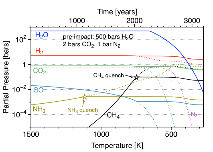
Figure 1: Example of quenching after a Vesta-sized impact into an Earth with a pre-impact atmosphere containing 2 bars CO₂, 1 bar of N₂, and 1.85 oceans (500 bars) of liquid water. Cooling (time) marches monotonically from left to right. Quench points for CH₄ and NH₃ H₂-N₂-NH₃ are indicated with stars. Solid lines show quenched compositions while dotted lines extend the equilibria to temperatures colder than the quench point for gas phase reactions. Partial pressures are also affected by water condensation ($T<650$ K).

If an impact is too small to fully vaporize the ocean, the ocean remains cool and acts as a heat sink that competes with thermal radiation to space. In the relevant case, the impact leaves the atmosphere much hotter than the ocean and mostly made of H₂ and water vapor. The lower atmosphere will therefore be stable against convection. Under these conditions the flow of energy down to the ocean is limited by radiative transfer. To illustrate, compare the diffusive flux of downward radiation in the Eddington approximation (any astronomy textbook),

$$F_{\downarrow}={16\over 3}{\sigma_{B}T^{3}\over\kappa\rho}{dT\over dz},$$ (19)

to Earth’s net cooling rate $F_{ir}$. The gray approximation opacity of water vapor is $\kappa\approx 0.1$ cm²g^-1 (Nakajima et al., 1992). Assume 30 bars of 1100 K steam as an example, for which the density at the surface is $\rho=0.025$ g cm^-3 and the surface temperature is 500 K (both set by the boiling point). The temperature gradient appropriate to cooling the whole atmosphere is $600\,(=\!\!1100-500)$ K over a 20 km scale height. With ${dT/dz}=3\times 10^{-4}$ K cm^-1, we estimate that $F_{\downarrow}\approx 0.5\times 10^{5}$ ergs cm^-2s^-1, which is 30% of net cooling ($F_{ir}$) to space. The radiative flux $F_{\downarrow}$ is relatively small because $\rho\kappa$ is big. (In this example, $F_{\downarrow}$ would exceed $F_{ir}$ for impacts that generate less than 10 bars of steam.) We conclude that, in general, relatively little of the energy in a hot deep steam atmosphere will flow downward to the ocean. The chief exception would be if there is enough CO₂ that the much hotter atmosphere is nonetheless dense enough to sink in cooler steam. This might happen for smaller impacts in deep CO₂ atmospheres, and if it did, it would result in complications that we will not address here.

3.4 Results

We consider three classes of impact.

(i) If the impact is big enough, it delivers enough iron to fully reduce all the H₂O and CO₂ at the surface. Under these conditions, the $\mathrm{Fe}+\mathrm{H}_{2}\mathrm{O}\leftrightarrow\mathrm{FeO}+\mathrm{H}_{2}$ equilibrium is likely to govern the oxidation state of the atmosphere throughout the cooling phase. Earth’s maximum HSE impact was in this size range. The iron-wüstite (IW) buffer describes the simple reaction of iron and steam to make FeO (wüstite) and H₂, and so is likely to be kinetically favored in the short term. On longer timescales the more reducing quartz-fayalite-iron buffer (QFI, effectively a buffer between iron and olivine) may dominate. Both mineral buffers favor CH₄, but the QFI buffer would also consume most of the H₂O in favor of H₂. The latter outcome resembles the story proposed to explain the desiccation of Mars by Dreibus and Wänke (1989); Kuramoto (1997).

A caveat is that, for impacts of this scale, the global ejecta blanket should have been tens of kilometers thick. Although the molten iron in the ejecta must have passed through the atmosphere and ocean to reach the surface — Genda et al. (2017b) estimate that more than half the iron is initially disseminated as mm-sized droplets — it is plausible that some of the iron was buried before it could react with H₂O or CO₂. If so, some of the reducing power of the impact would at first have been sequestered from the surface, only becoming available as reduced gases emitted to the atmosphere on a longer geologic timescale. Modeling the fate of iron in the post-impact mantle is beyond the scope of this study.

(ii) The oceans are fully vaporized but there isn’t enough metallic iron in the impact to reduce all of the H₂O in the ocean to H₂. Impacts on this scale leave much of the H₂O and CO₂ unreacted. In such an impact the ejecta blanket is not much thicker than the ocean is deep, and conditions at the surface are supercritical for water, promoting efficient chemical coupling of the water with the iron while the iron lasts (see Choudhry et al., 2014, and references therein). There are of the order of ten such impacts in a representative maximum late veneer, and 1-3 in a minimum late veneer. We assume that in these events the introduced Fe consumes oxygen from the water and CO₂ until the all the injected Fe is gone. Thereafter the atmosphere evolves with its oxygen content (in H₂O, CO, and CO₂) held constant. In these events the steam atmosphere is deep, thick, and hot, and cooling is slow, conditions that strongly favor CH₄ and, to a lesser degree, NH₃.

(iii) The impact is too small to fully vaporize the oceans. These events feature faster cooling times and lower atmospheric pressures, with the amount of steam generated proportional to the energy released by the impact. The lower pressures are generally much less favorable to CH₄ formation, but small impacts are interesting because there are more of them and they are likelier to be survived by life or its precursors. For small impacts, we will find that the QFM mineral buffer often generates a more reduced gas composition than predicted from scavenging by impact iron of the oxygen in the hydrosphere and atmosphere. For these events we will presume that the ferrous iron already present in the crust is available as an additional sink of oxygen at the QFM buffer. These matters are discussed in more detail below.

We treat the volume of the ocean and the amount and state of carbon in the atmosphere before the impact as initial conditions. For water, we assume that 1.85 oceans of water (5 km) were present at the surface. Bigger oceans allow for more extensive loss of hydrogen to space without desiccating the planet. We take the view, provisionally, that a much drier planet ($\ll$1 ocean) will not evolve to Earth as we know it.

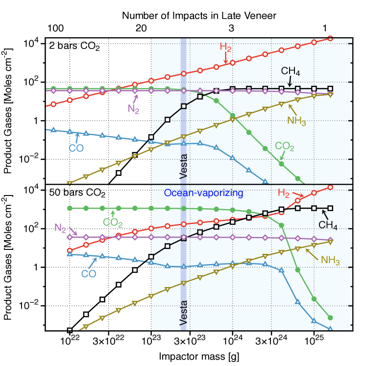
Figure 2: Quenched impact-induced transient atmospheres as a function of impactor mass (EH composition) for two pre-impact atmospheres, one with 50 bars of CO₂ and the other with 2 bars. Both have 1 bar of N₂ and 1.85 oceans (500 bars) of water on the surface. Inventories are shown in moles to highlight the chemical transformation. A Vesta-size impact is indicated by the shaded vertical bar. Potentially ocean-vaporizing impacts are indicated by lighter shading. A rough guide to the number of impacts of a given size is listed across the top. In these models, all reducing power is furnished by the quantitive reduction of the impactor’s Fe to FeO; no mineral buffering is assumed. In the maximum late veneer impact (at right), nearly all CO and CO₂ are converted to CH₄.

Carbon reservoirs are not well constrained. Between surface, crust, and mantle, Earth may hold the equivalent of $200\pm 100$ bars of CO₂ (Sleep and Zahnle, 2001; Dauphas and Morbidelli, 2014). One end-member is hot and oxidized, with CO₂ being initially divided roughly equally between a melted QFM mantle and Henry Law partitioning of 100 bars of CO₂ in the atmosphere in the aftermath of the Moon-forming impact (Holland, 1984; Abe, 1997; Zahnle et al., 2007; Elkins-Tanton, 2008). An oxidized mantle could have been consequent to a previous history of hydrogen escape or to iron-mineral disproportionation (Frost and McCammon, 2008). CO₂ can also be generated from thermal decomposition of carbonate minerals if these were near the surface. Although we do not explicitly consider more reduced atmospheres (CO or CH₄) as initial conditions, we will find below that thick CO or CH₄ atmospheres can be long-lasting in the Hadean. The CO₂ atmosphere is the most oxidized and hence the most conservative case. We treat $p_{\mathrm{CO}_{2}}$ as a free parameter.

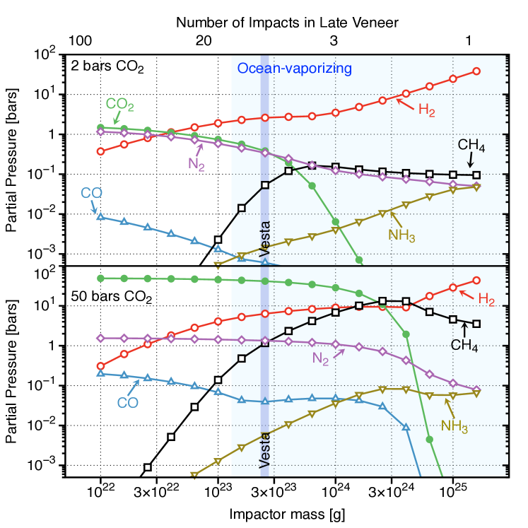
Figure 3: Same as Figure 2, but atmospheric compositions shown as partial pressures.

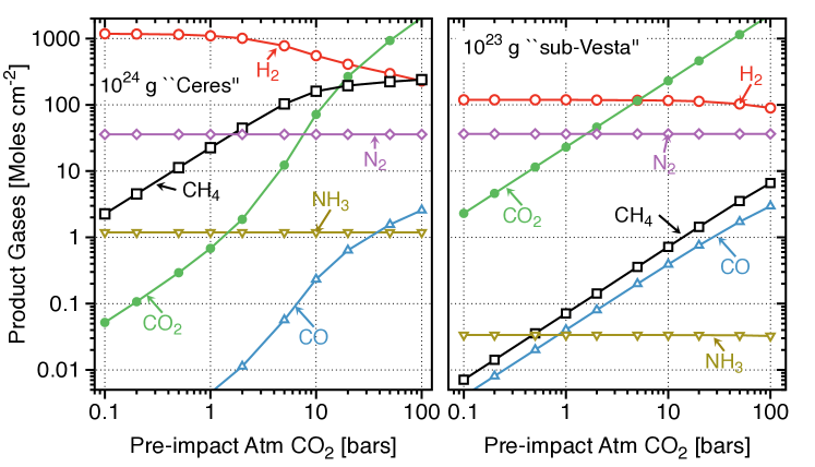
Figure 4: Quenched impact-induced transient atmospheres as a function of how much CO₂ was in the atmosphere before the impact, for two sizes of impact, one ocean-vaporizing, one not. The pre-impact Earth has 1 bar of N₂ and 1.85 oceans (500 bars) of water on the surface. The Ceres-sized ($10^{24}$ g) impact (EH) is big enough to convert thinner CO₂ atmospheres to CH₄, but hasn’t enough Fe to fully reduce the thicker CO₂ atmospheres. The smaller “sub-Vesta” impact is too small to fully vaporize 1.85 oceans; the chief effect is to make a lot of H₂.

Table 1 lists a sampling of possible Hadean impacts. Before impact, Earth is presumed to have had 1.85 oceans of water at the surface (500 bars, 28.3 kmols cm^-2) and one bar (36 moles cm^-2) of N₂ in the atmosphere. The amount of CO₂ varies between examples. “100 bars” of CO₂ corresponds to 2300 moles cm^-2.

Figures 2 and 3 show post-impact atmospheres for a wide range of impact sizes for 2 and 50 bars of CO₂. Figure 2 shows column densities (moles cm^-2), which makes the chemical trends clear, while Figure 3 shows the same information as partial pressures. The reducing power of the impactors presumes high iron EH (enstatite) or H (ordinary) chondritic bodies (33% Fe by mass, which also approximates the bulk Earth). Impact energy assumes an impact velocity of 17 km s^-1. Table 1 lists major product gases for each case. Many of the cases listed in the table are used as initial conditions for photochemical evolution in Section 3 below. If the Fe is incompletely used up, the corresponding impact mass can simply be scaled up; i.e., if half the Fe goes unreacted, the required impactor would have twice the mass.

The maximum HSE impact delivers marginally enough Fe to fully reduce the atmosphere and hydrosphere, which suggests that equilibration with a mineral buffer may be plausible. Table 1 lists several maximum HSE cases with 100 bars of CO₂ equilibrated to different buffers. The QFI buffer, which would also fully reduce the atmosphere and hydrosphere, seems likeliest if the reactions all go to completion. But if much of the iron is buried before it reacts, a more oxidized buffer might be more reasonable.

In the next category, the “Pretty Big” cases approximate the biggest impact in our lower bound late veneer, whilst “Ceres” and “Vesta” are impacts with the mass of the real Ceres and the real Vesta. These are all ocean-vaporizers, but none deliver nearly enough iron to fully reduce the ocean. Figure 4 compares outcomes as a function of $p$CO₂ for Ceres-sized impacts.

The third category is represented in Table 1 by two “sub-Vestas” and the lunar South Pole-Aitken impact that do not fully evaporate the oceans. These are small enough that life or its precursors might survive. These impacts are also too small to deliver enough metallic iron to reduce the ocean to the QFM composition. This means that the reducing power of Earth’s mineral buffers — made active by the heat of the impact — needs to be taken into account. The South Pole-Aitken basin is an example of a relatively minor event.

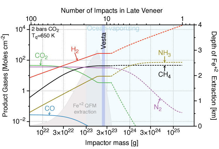
Figure 5: The left-hand axis shows gas compositions as a function of impact mass when quenching is assumed to take place at 650 K (water’s critical temperature). Solid lines for smaller impacts ($M_{i}<4\times 10^{23}$ g) show gas compositions in equilibrium with the QFM mineral buffer. The right-hand axis shows the depth (shading) to which FeO in the crust must be oxidized to magnetite (Fe₃O₄) to maintain equilibrium with the QFM buffer at 650 K. Dashed lines for gas compositions generated by bigger impacts ($M_{i}>4\times 10^{23}$ g) are determined by metallic iron delivered by the impact. These latter compositions are no more reduced than the otherwise comparable compositions seen for gas phase quenching in Figure 2 above, but the assumed low 650 K quench temperature favors CH₄ and NH₃ over H₂.

Table 1 lists two sub-Vestas. The first uses only the reducing power of the impact. This is the most pessimistic case. The other assumes equilibration with a crustal QFM mineral buffer, but at an arbitrary lower quench temperature of 650 K. In effect, the second case asks what happens if supercritical water was in itself enough to ensure that the coupled H₂-H₂O-CO-CO₂-CH₄-N₂-NH₃ system equilibrated on a thousand year time scale. This can be viewed as the optimistic limit on what sub-ocean-vaporizing impacts can do to generate species like CH₄ and NH₃.

Figure 5 illustrates the potential inherent in the more optimistic case. Here we assume that the atmosphere and ocean remain chemically equilibrated with the crust or mantle at the QFM buffer while water remains supercritical; i.e., we set $T_{q}=650$ K. The QFM buffer is only weakly reducing because it has only Fe⁺² to offer as a reductant. On the other hand there is a great deal of Fe⁺² available in impact-heated crust and mantle materials, although the crustal source is not inexhaustible.

To illustrate these considerations, in Figure 5 we estimate the depth in the crust (global average) to which FeO must be oxidized to Fe₃O₄ (magnetite), assuming that the crust was 10% FeO by mass and that all the FeO is oxidized to Fe₃O₄, and taking into account the reducing power delivered by the impact as metallic iron. Figure 5 presumes a pre-existing atmosphere with the equivalent of 2 bars of CO₂ and one bar of N₂. The figure shows that, even in a Vesta-scale impact, the required reducing power can be extracted from FeO in the uppermost 3 km of a QFM crust. Smaller impacts use less of Earth’s FeO because they don’t evaporate the entire ocean, while larger impacts (larger than $4\times 10^{23}$ g in Figure 5) deliver more metallic iron than needed to maintain QFM.

4 Photochemical evolution of impact-generated transient atmospheres

Our goal in this Section is to model the photochemical decay of the impact-generated transient reduced atmosphere. In particular we are interested in what happens to methane. The key processes driving the atmosphere’s evolution are ultraviolet photolysis and hydrogen escape. Thus, fundamentally, we are most concerned with counting the photons and apportioning their effects.

4.1 The Photochemical Model

In the photochemical model, we consider six major species: H₂, CH₄, H₂O, CO₂, CO, and N₂. Minor species include HCN (nitriles), C₂H_n (a mix of C₂H₂, C₂H₄, C₂H₆), and organic haze. Other molecules and free radicals that are considered include NO, NH, N(⁴S), N(²D), O(³P), O(¹D), ³CH₂, ¹CH₂, CH₃, and OH. We refer to ground state N(⁴S) as N, ground state O(³P) as O, and ground state ³CH₂ as CH₂. Key reactions are listed in Appendix B. Atomic H is implicit and lumped with H₂ for accounting purposes. Ions are not explicitly included, although the first order effects of ion chemistry are taken into account as loss processes for CO₂ and CH₄ (Appendix C).

Our purpose is to construct the simplest model that captures the first order consequences of photochemical evolution of unfamiliar atmospheres, while conserving elements and counting the photons. Anything more complicated (e.g., a 1-D atmospheric photochemistry code) would necessarily introduce several poorly-constrained free parameters. We therefore assume that the major atmospheric constituents are uniformly distributed vertically, affected only by the totality of chemical and physical sources and sinks. We treat each major species $j$ as a column density $N_{j}$ (units of number per cm²). Ultraviolet photons are sorted into several spectral windows and the effects of photolysis are apportioned in accordance with the first order consequences of photochemistry; these simplifications will be discussed in detail below. The columns are evolved through time by integrating $dN_{j}/dt$. Hydrogen escape and the effectively irreversible photolysis of methane impose direction.

There are two first order complications to the simplest model that demand attention. First, H₂O — usually the most abundant gas after the impact — condenses to make oceans. Thereafter its abundance at stratospheric altitudes where photolysis takes place is limited by the atmosphere’s cold trap. Water vapor is key to these models because water vapor is often the major oxidant. The drier the stratosphere, the more slowly it evolves and the more likely it is to favor reduced products like hydrocarbons. A next generation study might investigate the water vapor contents of self-consistent radiative-convective atmospheres, but this level of modeling goes beyond the scope of this study. Here we treat stratospheric water vapor in the atmosphere as a free parameter.

The second complication is the shadow cast by organic hazes. Organic hazes are expected when methane is abundant and subject to UV photolysis (Trainer et al., 2006; Hörst et al., 2012, 2018b). The analogy is Titan. We expect Earth’s hazes, when present, to be optically thick, much thicker than on Titan today, because UV irradiation of early Earth was at least 1000 times greater than of modern Titan. Here we follow Wolf and Toon (2010) and parameterize haze optical depth as a function of haze production rate. Because water photolysis would be the major source of oxidants in a methane-rich atmosphere, the competition between hazes and water for UV photons creates a positive feedback in which one or the other dominates.

4.1.1 Irradiation

We divide the solar FUV and EUV spectrum into six windows that align with particular properties of the atmosphere (Table 4.1.1). We neglect the Lyman continuum (80-91.2 nm, current photon flux of $8\times 10^{9}$ cm^-2s^-1) as filtered out by atomic H. Absorption at wavelengths longer than the Lyman continuum usually leads to dissociation of molecules into two neutral species. Absorption at wavelengths shorter than the Lyman continuum usually ionizes the molecule, leaving the molecule provisionally intact as an ion.

The ancient Sun was a stronger source of EUV radiation than is the modern Sun. We scale the different channels according to the general rule that hotter source regions are relatively more enhanced by solar activity and were therefore relatively more enhanced when the Sun was young (Zahnle and Walker, 1982; Claire et al., 2012). Enhancement factors for the different windows are listed in Table 4.1.1.

Fluxes [cm^-2s^-1] and cross sections [cm²] Spectral Window EUV${}_{1}^{a}$ EUV${}_{2}^{b}$ EUV-N${}_{2}^{c}$ Lyman $\alpha$ FUV-CO₂ FUV-H₂O $i$ 1 2 3 4 5 6 $\lambda$ [nm] $<80$ $91.2\!-\!117$ $91\!-\!100$ $121.5$ $125\!-\!170$ $170\!-\!185$ $F_{\lambda}^{d}$ $3\!\times\!10^{10}$ $2\!\times\!10^{10}$ $3.6\!\times\!10^{9}$ $3.6\!\times\!10^{11}$ $4\!\times\!10^{11}$ $2.5\!\times\!10^{12}$ $S_{\lambda}^{e}$ $30$ $20$ $10$ $10$ $7$ $4$ $j$ Cross section $\sigma_{ij}$ [cm²] 1 H₂ $2\!\times\!10^{-18}$ $2\!\times\!10^{-18}$ – – – – 2 CH₄ $2\!\times\!10^{-17}$ $8\!\times\!10^{-18}$ $8\!\times\!10^{-18}$ $8\!\times\!10^{-18}$ – – 3 H₂O $1.3\!\times\!10^{-17}$ $8\!\times\!10^{-18}$ $8\!\times\!10^{-18}$ $8\!\times\!10^{-18}$ $1\!\times\!10^{-18}$ $3\!\times\!10^{-18}$ 4 CO₂ $2\!\times\!10^{-17}$ $4\!\times\!10^{-17}$ $4\!\times\!10^{-17}$ $5\!\times\!10^{-20}$ $8\!\times\!10^{-19}$ – 5 CO $1.3\!\times\!10^{-17}$ – – – – – 6 N₂ $1.3\!\times\!10^{-17}$ – $2.5\!\times\!10^{-16}$ – – – $a$ – Photo-ionizing EUV excluding the Lyman continuum $b$ – EUV₂ excludes photoionizing radiation and radiation that photolyzes N₂ $c$ – EUV-N₂ is the portion of non-photoionizing EUV that coincides with N₂ absorption $d$ – Quiet Sun irradiance, photons cm^-2s^-1 at 1 AU $e$ – Young Sun enhancement over modern quiet Sun

Total column photolysis rates $\Phi_{j}$ [cm^-2s^-1] for species $j$ allow for competition for photons between species,

$$\Phi_{j}=\frac{1}{4}\sum_{i=2,6}F_{i}S_{i}{\sigma_{ij}N_{j}\displaystyle\over\displaystyle\sum_{k=1,7}\sigma_{ik}N_{k}},$$ (20)

where $k$ is an index running over the species. This approach conserves photons, which is the principal requirement here. Photo-ionization is treated separately,

$$\Phi^{\ast}_{j}=\frac{1}{4}F_{1}S_{1}{\sigma_{1j}N_{j}\over\sum_{k}\sigma_{1k}N_{k}}.$$ (21)

Organic hazes when present may provide UV protection to the deeper atmosphere (Sagan and Chyba, 1997; Pavlov et al., 2001; Wolf and Toon, 2010). Wolf and Toon (2010) constructed a microphysical model of organic hazes of early Earth. They considered spherical haze particles and “fractal” haze particles, with the latter model much preferred by its authors. We fit power laws to the fractal haze optical depths listed in their Table S1 as a function of the haze production rate,

$$\tau_{uv}\approx 10\left(dN_{\mathrm{haze}}/dt\over 3\times 10^{10}\right)^{0.8}$$ (22)

and

$$\tau_{vis}\approx 0.5\left(dN_{\mathrm{haze}}/dt\over 3\times 10^{10}\right)^{0.7}.$$ (23)

The ultraviolet optical depth refers to 197 nm and the visible optical depth refers to 564 nm. We have converted units from production in grams per year to the equivalent number of carbon atoms cm^-2s^-1, which are the units used in this paper. Haze production rates on early Earth can exceed $1\times 10^{12}$ carbon atoms cm^-2s^-1, which corresponds to UV and visible fractal haze optical depths of the order of 160 and 6, respectively.

Hazes can suppress H₂O photolysis if the stratosphere is dry. This can lead to a positive feedback that encourages haze formation. As hazes thicken, there is less H₂O photolysis and less oxidation, which favors more haze formation. The consequence of this positive feedback resembles a phase change, in which much of the carbon derived from methane photolysis polymerizes into a wide range of heavier, generally oxygen-deficient organics (which we loosely refer to as “haze”) that precipitate to the troposphere and probably to the surface.

In wetter stratospheres, haze formation competes with oxidation consequent to H₂O photolysis. The organics and hazes that form under these conditions will contain more oxygen, suggesting a relatively greater role for acids, aldehydes, carbonyls, and other more water-soluble molecules that are more likely to rain out when they reach the troposphere. These may be essential ingredients for genesis of ribose for the RNA world (cf., Benner et al., 2019b).

4.1.2 Photolysis

Methane photolysis is dominated by Lyman $\alpha$ radiation. Methane photolysis at Lyman $\alpha$ mostly yields an excited methylene radical ¹CH₂ plus hydrogen (Huebner et al., 1992). Singlet methylene can be collisionally de-excited to the less reactive triplet ³CH₂, or it can react with CH₄ or H₂ to make CH₃ radicals. We will refer to these small radicals generically as CH_n. Both CH₂ and CH₃ react very quickly with atomic N from N₂ photolysis to make C-N bonds or with atomic O from CO₂ photolysis to make C-O bonds. The C-O bonds once formed are difficult to break photochemically. The N reactions are the primary sources of HCN in a CH₄-N₂ irradiated atmosphere. We neglect the possible catalytic role of N₂ through the CH₂N₂ (diazomethane) intermediary.

Competition for Ly $\alpha$ photons is limited. We do not expect scattering by atomic hydrogen to be significant, because the solar Ly $\alpha$ emission is much broader than the velocity dispersion in hydrogen atoms at atmospheric temperatures. CO₂ has a very small cross section to Ly $\alpha$, only about 0.5% of methane’s. Both H₂ and CO have hot absorption lines that partially overlap with Lyman $\alpha$ emission. Resulting fluorescence has been seen in planetary nebulae (Lupu et al., 2006) and cometary comae (Lupu et al., 2007), respectively. However, the effect requires ro-vibrationally excited H₂ and CO molecules, and hence is unlikely to be important at relevant conditions. Water’s cross section at Ly $\alpha$ is about the same as methane’s, but we do not expect H₂O to be abundant at the highest altitudes once the cold trap has been established in the lower atmosphere. What this all means is that, when methane is abundant, Ly $\alpha$ photochemistry takes place high in the atmosphere, aligning it with N₂ photolysis and generally favoring the production of organic hazes and nitriles. When methane is not abundant, Ly $\alpha$ photochemistry takes place deeper in the atmosphere, which better aligns methane photolysis with CO₂ photolysis and H₂O photolysis, an alignment that favors methane oxidation and disfavors nitrile production.

Nitrogen (N₂) photolysis is dominated by several very strong narrow absorption bands that coincide with solar emission lines. Huebner et al. (1992) stresses the importance of the overlap between a strong N₂ band and solar Ly $\gamma$ (92.25 nm). Comparison between the solar spectrum (Curdt et al., 2001) and the N₂ absorption spectrum predicted by Liang et al. (2007), Li et al. (2013), and Heays et al. (2014) shows that strong N₂ absorption bands coincide with several other Lyman lines, including Ly $\delta$ (94.974 nm), Ly $\epsilon$ (93.78 nm), Ly 7, 8, and 12, and also with an NIII line (99.17 nm). There is also overlap at 91.3 nm where Lyman lines ($n\!>\!30$) pile up in the approach to the Lyman limit. Huebner et al. (1992) estimated from a suite of discordant experiments that the N₂ photolysis cross section at Ly $\gamma$ is of order $2.5\times 10^{-16}$ cm².

Nitrogen’s chief competition for photons is with CO₂, which has big cross sections of order $4\times 10^{-17}$ cm² at wavelengths where N₂ absorbs. Molecular hydrogen also absorbs at some of these wavelengths, Ly $\gamma$ in particular, but cross sections are generally smaller than $10^{-18}$ cm². For the quiet Sun at Earth, we estimate a total N₂ photolysis rate of $3.6\times 10^{9}$ cm^-2s^-1, which agrees well with what Liang et al. (2007, their Figure 2) compute for Titan when scaled to 1 AU.

Photolysis between 91.2 nm and 100 nm splits N₂ into a ground state N atom and an electronically excited $\mathrm{N}(^{2}\mathrm{D})$. The $\mathrm{N}(^{2}\mathrm{D})$ can react with H₂ or CH₄ to make NH, react with CH₄ to make CH₂NH, and react with CO₂ to make CO and NO (Herron, 1999). Both NH and NO react rapidly with N to reconstitute N₂. Otherwise the most important N and NH reactions are with hydrocarbon radicals to make HCN and other nitriles, such as acetonitrile (CH₃CN) and cyanoacetylene (HCCCN). Photolytic production of HCN has been predicted to work well in an N₂-CO₂ atmosphere (Zahnle, 1986; Tian et al., 2011). Photochemical organics have been hypothesized as a source of reduced nitrogen and reduced carbon that can be subducted by the mantle (Wordsworth, 2016).

At the top of the atmosphere, CO₂ photolysis is dominated by EUV wavelengths between 91.2 nm (the Lyman limit) and 115 nm. Weaker absorption at FUV wavelengths between 130 nm and 180 nm can be as important if other absorbers are not abundant. At FUV wavelengths, CO₂ photolysis usually creates a ground state CO molecule and a highly reactive O(¹D) atom.

$$\mathrm{CO}_{2}+h\nu\rightarrow\mathrm{CO}+\mathrm{O}(^{1}\mathrm{D})$$ (24)

At the shorter wavelengths, photolysis can also yield electronically excited CO and a ground state O atom (Huebner et al., 1992). We will assume that excited CO is de-excited by collisions.

The $\mathrm{O}(^{1}\mathrm{D})$ atom is highly reactive, including reaction with CH₄ to liberate CH₃. Key $\mathrm{O}(^{1}\mathrm{D})$ reactions are listed in Appendix B. It can be de-excited to the less reactive $\mathrm{O}(^{3}\mathrm{P})$ ground state by collisions with CO₂, N₂, and CO, but it reacts quickly with CH₄ and H₂. By contrast, reactions of ground state O with CH₄ and H₂ are negligibly slow at 300 K. We therefore take the initial reaction of $\mathrm{O}(^{1}\mathrm{D})$ with CH₄ as the rate-limiting step for CH₄ loss from CO₂ photolysis. Subsequent reactions of O with free radicals like CH₃ are fast and result in CO bonds.

Carbon monoxide has a similar spectrum to N₂, but unlike N₂, few of its bands align with strong solar emission lines. CO dissociation into neutral atoms is dominated by the Lyman continuum (Huebner et al., 1992), and hence is relatively unimportant in hydrogen-rich atmospheres.

Water photolysis yields OH and H for FUV with $\lambda<190$ nm. If the stratosphere is very dry, organic hazes have potential to shield H₂O from photolysis, especially at wavelengths $\lambda>182$ nm, where H₂O’s cross section starts to fall off rapidly with increasing $\lambda$.

Because we do not distinguish between H and H₂, hydrogen photolysis is important only as opacity.

Ammonia is swiftly photolyzed by UV radiation between $185<\lambda<215$ nm at wavelengths where H₂O and CO₂ absorptions are very weak. The products are highly reactive NH and NH₂ radicals (Huebner et al., 1992). These can lead to N₂ formation, but they can also react with hydrocarbons if the latter are plentiful.

4.1.3 The methane budget

Methane ends up either as organics or HCN, or is oxidized to CO or CO₂. While CH₄ is preponderant, photochemistry following photolysis will tend to generate hydrocarbons (Lasaga et al., 1971; Yung and Pinto, 1978; Zahnle, 1986; Trainer et al., 2006; Hörst et al., 2018b) and nitrogenous organics. When CO₂ is preponderant, methane is more often oxidized to formaldehyde (HCHO) or CO.

Methane can also be oxidatively attacked by products of H₂O photolysis and CO₂ photolysis. The most important of these are O(¹D) atoms from CO₂ photolysis (R32) and OH from H₂O photolysis or reaction of O(¹D) with H₂. (Reactions of CH₄ with H and ground state O atoms are slow unless the gas is much hotter than we have assumed, while reaction with N(²D) typically creates nitriles.) OH reacts fairly rapidly with CO to make CO₂, and more slowly at room temperature with H₂ or CH₄ to yield H₂O. The reactions of OH with H₂ and CH₄ are sensitive to temperature, whilst the reaction with CO is not. At 300 K, $\mathrm{OH}+\mathrm{CO}\rightarrow\mathrm{CO}_{2}$ is about $20\times$ faster than reaction with H₂ or CH₄, and at 250 K its about $100\times$ faster.

Column oxidative loss of CH₄ is approximated by loss reactions with O(¹D) from CO₂ photolysis and OH from H₂O photolysis:

$$\left({dN_{\mathrm{CH}_{4}}\over dt}\right)_{\!\!ox}=-\Phi_{\mathrm{CO}_{2}}\left({k_{22}N_{\mathrm{CH}_{4}}\over\sum_{j}k_{2j}N_{j}}\right)-\Phi_{\mathrm{H}_{2}\mathrm{O}}\left({k_{32}N_{\mathrm{CH}_{4}}\over\sum_{j}k_{3j}N_{j}}\right).$$ (25)

The total CH₄ budget sums the photolytic, photoionic, and oxidative losses,

$${dN_{\mathrm{CH}_{4}}\over dt}=-\Phi_{\mathrm{CH}_{4}}+\left({dN_{\mathrm{CH}_{4}}\over dt}\right)_{\!\!ions}+\left({dN_{\mathrm{CH}_{4}}\over dt}\right)_{\!\!ox}.$$ (26)

4.1.4 Hydrocarbons and organic hazes

Reactions between CH, CH₂ and CH₃ lead to acetylene, ethylene, ethane, and eventually to more complicated hydrocarbons that can form a high altitude haze. The chief competing reactions are those with O or OH radicals. We lump acetylene, ethylene, and ethane together as C₂H_n hydrocarbons. We equate the creation of CH_n radicals to the appropriate destruction rate of CH₄,

$$\frac{dN_{\mathrm{CH}_{n}}}{dt}=\Phi_{\mathrm{CH}_{4}}-\left(\frac{dN_{\mathrm{CH}_{4}}}{dt}\right)_{\!\!ions}-\left(\frac{dN_{\mathrm{CH}_{4}}}{dt}\right)_{\!\!ox}\geq 0.$$ (27)

We equate the production of oxidizing radicals in the haze-forming regions to the appropriate photolysis rates of H₂O and CO₂,

$$\frac{dN_{\mathrm{ox}}}{dt}=\Phi_{\mathrm{CO}_{2}}+\Phi^{\!\ast}_{\mathrm{CO}_{2}}+\Phi_{\mathrm{H}_{2}\mathrm{O}}\geq 0.$$ (28)

We assume that C₂H_n molecules form when a CH_n radical reacts with another CH_n radical, while CO forms when a CH_n radical reacts with an O or OH radical,

$$\frac{dN_{\mathrm{C}_{2}\mathrm{H}_{n}}}{dt}=\frac{1}{2}\frac{dN_{\mathrm{CH}_{x}}}{dt}\left(dN_{\mathrm{CH}_{x}}/dt\over dN_{\mathrm{ox}}/dt+dN_{\mathrm{CH}_{x}}/dt\right)^{\!2}.$$ (29)

Organic hazes form when several CH_n radicals react with the growing polymer for each reaction with an O or OH,

$$\frac{dN_{\mathrm{haze}}}{dt}=\frac{dN_{\mathrm{CH}_{x}}}{dt}\left(dN_{\mathrm{CH}_{x}}/dt\over dN_{\mathrm{ox}}/dt+dN_{\mathrm{CH}_{x}}/dt\right)^{\!m}.$$ (30)

For specificity we take $m\!=\!5$ (corresponding to six carbons). For accounting purposes we assume that all hazes fall to the surface and accumulate without further reaction,

$$N_{\mathrm{haze}}=\int\frac{dN_{\mathrm{haze}}}{dt}dt.$$ (31)

Hazes are generally ineffective at shielding molecules from photolysis at wavelengths where an abundant gas absorbs strongly, because hazes make up a very small mass fraction of the atmosphere. Where hazes can matter is in shielding a gas of very low abundance at wavelengths that would otherwise be transparent. The cases of interest here are H₂O, which can be cold-trapped, and NH₃.

4.1.5 CO and CO₂ budgets

The CO₂ budget is a balance between photolytic losses and CO oxidation,

$${dN_{\mathrm{CO}_{2}}\over dt}=-\Phi_{\mathrm{CO}_{2}}\left(1-f_{2x}f_{35}\right)-\Phi_{\mathrm{CO}_{2}}^{\ast}+f_{35}\Phi_{\mathrm{H}_{2}\mathrm{O}}+\Phi_{\mathrm{CO}_{2}}\left(1-f_{2x}f_{45}\right)$$ (32)

where $f_{2x}$ denotes the fraction of O(¹D) that react with other atmospheric species to create OH radicals,

$$f_{2x}\equiv{k_{21}N_{\mathrm{H}_{2}}+k_{22b}N_{\mathrm{CH}_{4}}+2k_{23}N_{\mathrm{H}_{2}\mathrm{O}}\over\sum_{j}k_{2j}N_{j}},$$ (33)

$f_{35}$ is the fraction of OH radicals that react with CO,

$$f_{35}\equiv{k_{35}N_{\mathrm{CO}}\over\sum_{j}k_{3j}N_{j}},$$ (34)

and $f_{45}$ is the fraction of ground state O atoms that react with CO to make CO₂,

$$f_{45}\equiv{k_{45}N_{\mathrm{CO}}\over\sum_{j}k_{4j}N_{j}}.$$ (35)

The latter reaction, although spin-forbidden, is important at high pressure in a dry CO-rich atmosphere in the absence of catalysts.

The CO budget reverses the CO₂ budget, and also includes the net oxidation of CH₄ as a source,

$${dN_{\mathrm{CO}}\over dt}=-{dN_{\mathrm{CO}_{2}}\over dt}-{dN_{\mathrm{CH}_{4}}\over dt}-{dN_{\mathrm{haze}}\over dt}-{dN_{\mathrm{HCN}}\over dt},$$ (36)

while treating precipitation of organic hazes and nitriles as a carbon sink.

This model of CO and CO₂ gives a better description of the sum of CO and CO₂ than it does of CO and CO₂ individually. Within the model, speciation between CO and CO₂ is sensitive to H₂O (the only oxidant). We suspect that our model overpredicts CO at the expense of CO₂.

4.1.6 Nitrogen and HCN budgets

In the anoxic atmospheres relevant to this study, nitrogen chemistry leads either to nitriles (e.g., HCN) or to the reconstitution of N₂. The direct products of nitrogen photolysis are

$${dN_{\mathrm{N}}\over dt}=\Phi_{\mathrm{N}_{2}}\left(1+{k_{15}N_{\mathrm{CO}}+k_{16}N_{\mathrm{N}_{2}}\over\sum_{j}k_{1j}N_{j}}\right),$$ (37)

$${dN_{\mathrm{NO}}\over dt}=\Phi_{\mathrm{N}_{2}}{k_{13}N_{\mathrm{H}_{2}\mathrm{O}}+k_{14}N_{\mathrm{CO}_{2}}\over\sum_{j}k_{1j}N_{j}},$$ (38)

$${dN_{\mathrm{NH}}\over dt}=\Phi_{\mathrm{N}_{2}}{k_{11}N_{\mathrm{H}_{2}}+k_{12b}N_{\mathrm{CH}_{4}}\over\sum_{j}k_{1j}N_{j}},$$ (39)

and

$${dN_{\mathrm{H}_{2}\mathrm{CN}}\over dt}=\Phi_{\mathrm{N}_{2}}{k_{12a}N_{\mathrm{CH}_{4}}\over\sum_{j}k_{1j}N_{j}}.$$ (40)

The H₂CN radical leads to HCN. Reaction paths through NO and HNO end in reactions with N that reconstitute N₂. These are the most important paths when CO₂ is abundant. The NH radical can be important when H₂ is very abundant, but under these circumstances NH is more likely to be recycled to N₂ than to react with CH_n to form C-N bonds. Ground state N reacts quickly with CH_n to make HCN, or if CH_n is not abundant it can be recycled to N₂ through reactions with NH or NO, or following reaction with OH. For most cases of interest here, OH is strongly suppressed by reactions with abundant CO or H₂.

Ammonia can be abundant after some impacts. As a placeholder, we assume that it is photolyzed.

$${dN_{\mathrm{NH}_{3}}\over dt}=-\Phi_{\mathrm{NH}_{3}}.$$ (41)

If methane is also abundant, ammonia photolysis probably leads to amines, but if H₂ is more abundant, ammonia photolysis will mostly end with reconstitution of N₂. The fraction of NH₃ photolyses that lead to amines or nitriles is approximated by

$$f_{99}={{dN_{\mathrm{CH}_{4}}/dt}\over{dN_{\mathrm{CH}_{4}}/dt}+\Phi_{\mathrm{H}_{2}\mathrm{O}}+\Phi_{\mathrm{CO}_{2}}}.$$ (42)

Reactions of NH_n with H₂ will reconstitute NH₃ and can be ignored. Efficient formation of cyanamide (NH₂CN) may require NH₃.

Net HCN, nitrile, and amine production is approximated by

$${dN_{\mathrm{HCN}}\over dt}=2\Phi_{\mathrm{N}_{2}}f_{1x}\left(dN_{\mathrm{CH}_{x}}/dt\over 2\Phi_{\mathrm{N}_{2}}f_{1x}+dN_{\mathrm{CH}_{x}}/dt\right)+f_{99}\Phi_{\mathrm{NH}_{3}}.$$ (43)

where $f_{1x}$ represents the fraction of excited N(²D) atoms produced that are available to make HCN,

$$f_{1x}={k_{12}N_{\mathrm{CH}_{4}}+k_{15}N_{\mathrm{CO}}+k_{16}N_{\mathrm{N}_{2}}\over\sum_{j}k_{1j}N_{j}}.$$ (44)

Equation 43 understates the possibility of NH reacting with organic species to make nitriles or amines. The corresponding net loss of N₂ by photolysis is

$${dN_{\mathrm{N}_{2}}\over dt}=-\Phi_{\mathrm{N}_{2}}+{1\over 2}{dN_{\mathrm{HCN}}\over dt}+{1\over 2}\Phi_{\mathrm{NH}_{3}}\left(1-f_{99}\right).$$ (45)

A convenient simplification is that these are reduced atmospheres with no net production of nitrogen oxides.

The chief chemical sinks of HCN are addition reactions with OH and H. The direct reaction with OH has an exothermic branch with products CO and NH₂, but the substantial rearrangements required to get these products require leaping over two energy barriers (Dean and Bozzelli, 2000). The climb over the first barrier gives, as one possible set of products, atomic H and HNCO (isocyanic acid). Addition reactions with H or CH_n can lead eventually to full hydrogenation through various intermediates including cyanamide and methlyamine. Like oxidation, these paths are expected to be kinetically inhibited.

The important physical sink is rainout. HCN is not very soluble in water (its Henry Law coefficient is not very high) but it is miscible. Total nitrile production is approximated by

$$N_{\mathrm{HCN}}=\int\frac{dN_{\mathrm{HCN}}}{dt}dt.$$ (46)

4.1.7 Hydrogen and hydrogen escape

The most important loss process for hydrogen is escape and its most important sources are CH₄ photolysis and oxidation, and water photolysis. Zahnle et al. (2019) found that, for a wide range of solar EUV fluxes and hydrogen mixing ratios, hydrogen escape from a terrestrial CO₂-H₂ atmosphere can be approximated by

$$\left(\frac{dN_{\mathrm{H}_{2}}}{dt}\right)_{\!\!esc}\approx-\frac{AS_{1}}{\sqrt{1+B^{2}S_{1}^{2}}}\frac{N_{\mathrm{H}_{2}}}{\sum_{j}N_{j}}\quad\mathrm{cm}^{-2}\mathrm{s}^{-1}.$$ (47)

where $A=2\times 10^{12}\mathrm{cm}^{-2}\mathrm{s}^{-1}$ and $B^{2}=0.006$. Here we use $S_{1}$ from Table 4.1.1 to scale EUV radiation to the levels appropriate to the young Sun. Equation 47 blends the energy-limited escape (the limit where $S_{1}$ is small) with the diffusion-limited escape (the limit where $S_{1}$ is large). Photochemical destruction of H₂ is not a concern for the hydrogen budget because in the diffusion limit H and H₂ escape almost equally easily.

Equation 47 is readily generalized to other planets and other atmospheric compostions by recognizing that $A$ is proportional to the density of the planet and $A\div B=b_{ia}\left(H_{a}^{-1}-H_{\mathrm{H}_{2}}^{-1}\right)$, where $H_{\mathrm{H}_{2}}$ and $H_{a}$ represent the unperturbed scale heights of H₂ and the background static atmosphere at the homopause, and $b_{ia}$ represents the binary diffusivity between H₂ and the background atmosphere. The latter is roughly the same for CO₂, CO, N₂, and CH₄ (Marrero and Mason, 1972). We can ignore $H_{\mathrm{H}_{2}}$ at this level of approximation. Thus, for Earth, $B\propto m_{a}\div m_{\mathrm{CO}_{2}}$, where the mean molecular mass of the static gases is

$$m_{a}={\sum_{j}N_{j}m_{j}-N_{\mathrm{H}_{2}}m_{\mathrm{H}_{2}}\over\sum_{j}N_{j}-N_{\mathrm{H}_{2}}}$$ (48)

Other things equal, the diffusion-limited hydrogen escape rate is about three times greater in CO₂ than in CH₄. We take the variation of $B$ as a function of $m_{a}$ into account in our models.

Sources of H₂ are photochemical or geological. The direct source is methane: each methane lost creates the equivalent of two H₂ molecules. Another source of H₂ is the water that oxidizes carbon from CH₄ to CO and CO₂. In evaluating this source we hold H₂O constant. The presumption is that water is in equilibrium with an ocean and resupplied to the stratosphere as needed. Some hydrogen is removed from the atmosphere when it is incorporated in precipitating organics and nitriles. For these we assume an H/C ratio of unity. The total rate of change of hydrogen is then

$$\frac{dN_{\mathrm{H}_{2}}}{dt}=\left(\frac{dN_{\mathrm{H}_{2}}}{dt}\right)_{\!\!esc}-2{dN_{\mathrm{CH}_{4}}\over dt}+2{dN_{\mathrm{CO}_{2}}\over dt}+{dN_{\mathrm{CO}}\over dt}-{dN_{\mathrm{haze}}\over dt}-{dN_{\mathrm{HCN}}\over dt}.$$ (49)

4.2 Photochemical Results

Here we present some illustrative examples of photochemical evolution for impacts of several scales.

4.2.1 Vestas

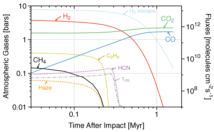
Figure 6: Photochemical dissipation of an atmosphere after the impact of a Vesta-sized body. The pre-impact atmosphere contained 5 bars of CO₂ and 1 bar of N₂ over 1.85 oceans (500 bars) of H₂O. This example assumes a dry ($1$ ppm H₂O) stratosphere. The optical depth of organic hazes at 564 nm $\tau_{vis}$ is shown against the left-hand axis. Production rates of HCN, C₂H_n species, and haze are plotted against the right-hand axis. The H₂ escape flux is also plotted against the right-hand axis. Note that in this case nitrile production (“HCN”) continues well after the other hydrocarbons have dissipated; the residual optical depth — of order unity at 250 nm — is from nitrogenous hazes.

A Vesta-scale impact is at the upper limit of what life might survive or prebiotic biomolecules might survive. Vesta itself is 525 km diameter, and has about 1% of the mass of the entire late veneer. There is energy enough to evaporate two oceans of water, which leaves few refugia unless the oceans were comparably enlarged.

Figure 6 shows evolution after a Vesta-size impact into a hefty pre-impact atmosphere holding 5 bars of CO₂ and 1 bar of N₂, and 1.85 oceans (500 bars) of H₂O. If all the Fe is used, the impact creates 3.9 bars of H₂ and converts about 9% of the 5 bars of CO₂ into CH₄ (see Table 1). Subsequent photochemical evolution assumes 1 ppm H₂O in the stratosphere, slightly drier than modern Earth’s. Production rates of HCN, C₂H_n species, and haze are roughly $30\times$ larger than those on modern Titan, or comparable to modern volcanic emissions of SO₂ or modern lightning production of NO. Cumulative precipitation of organics is about 5 cm. Hydrogen equivalent to 45 meters of a global ocean escapes to space over the course of the event.

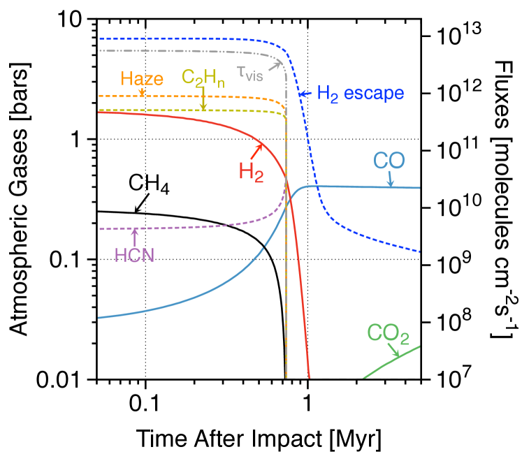
Figure 7: Photochemical evolution after a Vesta-size impact assuming that the atmosphere and ocean equilibrate with the QFM buffer at 650 K (see Figure 5). The pre-impact atmosphere contained 2 bars of CO₂, otherwise conditions are the same as for Figure 6. The case is listed in Table 1.

We estimate the surface temperature by assuming that the troposphere follows a moist adiabat, with the tropopause at the skin temperature,

$$T_{\mathrm{surf}}\approx\left(\left(1-A\right)SF_{\odot}\over 8\sigma_{B}\right)^{0.25}\left(p_{\mathrm{surf}}\over p_{\mathrm{tr}}\right)^{(\gamma-1)/\gamma}=180\left(p_{\mathrm{surf}}\over 0.1\;\mathrm{bar}\right)^{0.13}\,\mathrm{K}.$$ (50)

We put the tropopause at 0.1 bar as in most solar system planets with atmospheres (Robinson and Catling, 2014). The solar constant $F_{\odot}=1.36\times 10^{6}$ ergs cm^-2s^-1 and the Stefan-Boltzmann constant $\sigma_{B}=5.67\times 10^{-5}$ ergs cm^-2s^-1 K^-4. Earth’s modern surface temperature is recovered with albedo $A=0.3$ and $\gamma=1.15$. For early Earth, the young Sun is 72% as bright as the modern Sun ($S=0.72$). If we take $0.3<A<0.5$, the $\sim 6$ bar atmosphere (1.6 bars CO₂, 0.55 bar N₂, 3.9 bars H₂, 0.17 bar CH₄) implies a surface temperature $T_{\rm surf}\sim 320$ K. A proper radiative-moist-convective model would be required to provide better estimates of surface temperature and tropopause conditions.

Figure 7, a more productive scenario than Figure 6, is obtained if the reducing power of FeO in pre-existing mantle and crust is exploited by lowering the quench temperature to the critical point of water and imposing the QFM buffer, as discussed above in the context of Figure 5. For a Vesta-size impact striking 2 bars of CO₂, 1 bar of N₂, and 1.85 oceans (500 bars) of H₂O, the result is 1.8 bars of H₂ and conversion of more than 90% of the CO₂ into CH₄ and more than 10% of the nitrogen into ammonia (see Table 1). The subsequent photochemical evolution in Figure 7 assumes a dry 0.1 ppm H₂O stratosphere. Such dryness might be expected in a deep greenhouse atmosphere illuminated by the faint young Sun. Predicted production rates of HCN, C₂H_n species, and haze are roughly $1000\times$ larger than those on modern Titan for about 0.7 Myrs. Cumulative precipitation of organics is about 10 m. Hydrogen equivalent to 60 meters of a global ocean escapes to space over the course of the event.

4.2.2 A “pretty big” impact

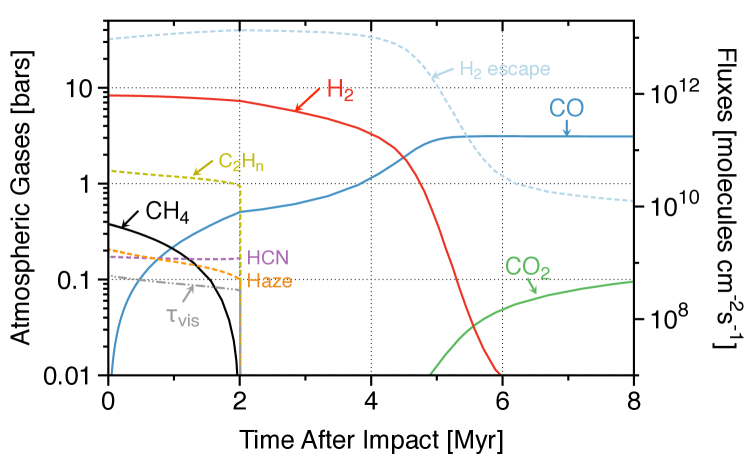
Figure 8: Photochemical dissipation of an atmosphere perturbed by a pretty big $2.5\times 10^{24}$ g impact. The pre-impact atmosphere contained 5 bars of CO₂ and 1 bar of N₂ over 1.85 oceans (500 bars) of H₂O. Partial pressures are shown against the left-hand axis. This example assumes $1$ ppm H₂O in the stratosphere, like Earth today. Production rates of hazes, C₂H_n species, and HCN are indicated against the right-hand axis. The H₂ escape flux is also plotted against the right-hand axis. Hydrogen from 50 bars (0.2 oceans, 500 meters) of H₂O escapes over the course of the event.

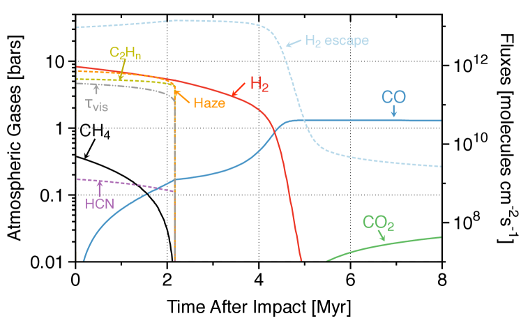
Figure 9: Same as Figure 8, but drier (0.1 ppm stratospheric H₂O). Organic hazes form with optical depths of order 3-5 at 564 nm ($\tau_{vis}$. Haze optical depth is plotted against the left-hand axis. In this example production rates of HCN and C₂H_n species, indicated against the right-hand axis, are very large, about $500\times$ what they are on modern Titan, or 2% of modern biotic productivity. Cumulative organic precipitation is of the order of 100 moles cm^-2.

Figures 8 and 9 document the profound influence of stratospheric moisture on atmospheric evolution after a bigger impact, here a “pretty big” $2.5\times 10^{24}$ g EH-type body striking a 5 bar CO₂, 1 bar N₂ atmosphere over 1.85 oceans (500 bars) of liquid H₂O. This approximates the largest event in a minimum late veneer extrapolated from the lunar cratering record, as discussed in Section 2 above. The surface temperature before the impact may have been in the range $310<T<340$ K (estimated using Eq. 50). There is enough energy released by the impact to vaporize 20 oceans of water or melt the crust to a depth of tens of kilometers. It seems unlikely that life on Earth could survive the immediate effects of an impact of this scale, but surface conditions ten thousand years later are plausibly temperate enough. This is an interesting scale for setting the table for life of the future (Benner et al., 2019a).

If all the new iron reacts with water and CO₂, this impact generates 8.4 bars of H₂ and converts nearly all of the 5 bars of CO₂ into 0.4 bars of CH₄. The mean molecular weight of the air is 3 and the scale height is 100 km. These are hydrogen atmospheres resembling Neptune’s more than modern Earth’s. Viewed in transit, such an atmosphere would add about 10% to Earth’s apparent diameter, or put another way, it would lead a distant observer to conclude that Earth had a density of just 4 g cm^-3.

The photochemical evolution in Figure 8 assumes 1 ppm H₂O in the stratosphere. The outcome is somewhat similar to that following the Vesta impact, differing mostly in the lack of CO₂. Most of the methane is eventually oxidized. A small fraction of the CH₄ is built up into organics, nitriles, and hazes. Production of HCN, hazes, and C₂H_n organics is roughly ten times faster than on modern Titan. Cumulative precipitation of hazes and nitriles is of the order of half a meter, with perhaps another half-meter of partially oxidized organic matter (e.g., organic acids and aldehydes stemming from partial oxidation of hydrocarbons). Hydrogen from 50 bars (0.2 oceans, 500 m) of H₂O escapes over 4 Myrs. Oxidation in the dry stratosphere is too slow to convert CO to CO₂ on the timescale of this event.

Figure 9 is the same impact as Figure 8, but evolving with a stratosphere that is ten times drier (0.1 ppm H₂O). The drier stratosphere might be appropriate given the strong greenhouse effect of the deep troposphere and the faint Sun. The outcomes are quite different. The low rates of stratospheric H₂O photolysis frustrate oxidation of small organics and thus allow the buildup of thick photochemical hazes ($\tau_{vis}\sim 5$ at 560 nm according to the fractal model). In this example, fully 60% of the impact-generated CH₄ is converted into organic precipitates (hazes), which correspond in cumulate to a global blanket 10-20 meters thick. On the other hand, production of organic nitrogen is no greater because in both case it is limited by the rate of N₂ photolysis. Conditions gradually grow less reducing until the methane is fully titrated and an abrupt bleaching event clears the skies. In the end, about 40% of the CH₄ is oxidized to CO, and the hydrogen from 0.15 oceans of H₂O escape to space.

4.2.3 The “maximum HSE” impact

Other things equal, there is a small but significant statistical chance, of the order of 10%, that the last of the world sterilizing events was also the biggest of them. Surface environments will not be habitable until well after the impact, but much can be done to prepare the planet for a more hopeful future. This approximates the impact discussed by Benner et al. (2019a).

We document two versions of a maximum HSE event, one with a very dry stratosphere and one somewhat moister. The simulations presume the impact on Earth of a highly-reduced Pluto-sized dwarf planet, at a time after the Moon-forming impact when there were still 100 bars of CO₂ at the surface. Other initial conditions are 1 bar of N₂ and 1.85 oceans of water (500 bars). The biggest impact differs from smaller impacts in two key respects: there is more iron than CO₂ and H₂O at the surface, and the ejecta blanket is much deeper than the oceans. The former means that the mineral buffer should be important, while the latter hints that much of the metallic iron might at first be buried.

For specificity we presume that the atmosphere and ocean equilibrate with the IW mineral buffer, and that the remaining metallic iron is oxidized later on geological time scales. With these particular assumptions, the impact converts all the CO₂ and 15% of the water to CH₄. About 60% of the water (one ocean) remains as H₂O. Expressed in moles, the atmosphere after the impact contains $6000$ moles H₂ per cm² (40% of the hydrogen in Earth’s current oceans) and $2300$ moles CH₄ per cm². Expressed as pressure, after the impact the dry atmosphere would at first hold 35 bars of H₂ and 14 bars of CH₄, with a mean molecular weight of 6. Because the surface temperature would be high, a great deal of water would remain in the vapor phase and the actual mean molecular weight and partial pressures of H₂ and CH₄ would be correspondingly higher.

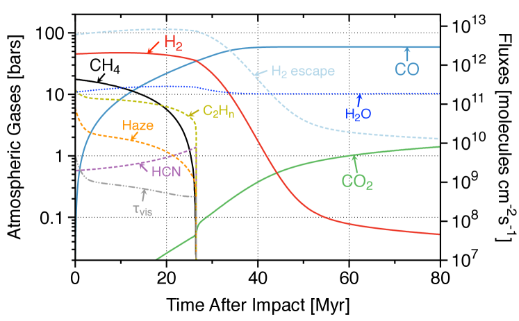
Figure 10: Photochemical evolution of a maximum HSE impact-generated atmosphere assuming 1 ppm H₂O in the stratosphere. Initial conditions (100 bars CO₂, 1.85 oceans of water) may be appropriate to the largest of Earth’s post-Moon impacts. Partial pressures are shown against the left-hand axis. Water vapor is mostly confined to the troposphere and presumes a surface temperature governed by total atmospheric pressure according to Eq 50. Organic C₂H_n, HCN, and haze production (dashed curves) are mapped to the right hand axis. The rate of hydrogen escape is also mapped to the right hand axis. Haze optical depth at 560 nm ($\tau_{vis}$) is plotted against the left-hand axis.

Figure 10 documents photochemical evolution with an Earth-like ($1$ ppm H₂O) stratosphere. As with the pretty big impacts, this stratosphere is moist enough that oxidation following water photolysis is more important than polymerization of CH₄. The photochemical source of organic matter (C₂H_n, HCN, haze) is nonetheless large, of the order of $100\times$ that of modern Titan. This case generates a cumulative global blanket of 25 m of haze organics, plus another 5 m of partially oxidized organics and 5 m of nitrogen-rich organics. Much of the nitrogenous material would be amines stemming from impact-generated NH₃. The hydrogen from 2.3 km of water escapes (leaving one ocean of water behind). Cases with still wetter stratospheres closely resemble this one.

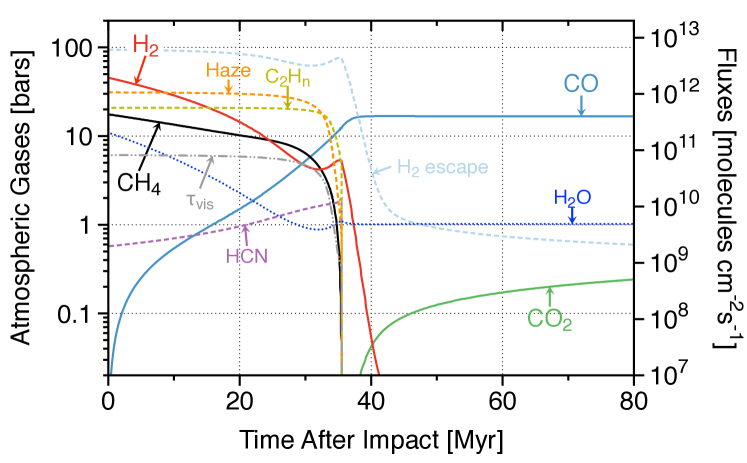
Figure 11: Same as Figure 10 but with a drier (0.1 ppm H₂O) stratosphere. Water vapor is mostly confined to the troposphere and presumes a surface temperature governed by total atmospheric pressure according to Eq 50. In this case the evolution is characterized by a very reduced stratosphere and a great deal of Urey-Miller-like abiotic organic production that consumes most of the CH₄. Organic (C₂H_n, HCN, and haze) production rates (dashed curves) are mapped to the right hand axis. Haze optical depth at 560 nm ($\tau_{vis}$) is plotted against the left-hand axis.

Figure 11 documents photochemical evolution with the drier ($0.1$ ppm H₂O) stratosphere. The dry stratosphere leads to highly reduced conditions and rapid photochemical organic haze production at $10^{3}\times$ the rate on modern Titan. Haze optical depths in the UV exceed 100; visible optical depths are in the range of 4-8. More than 70% of the methane is polymerized into organic matter equivalent to a cumulative deposit of the order of 300 to 500 m deep. In addition, about 10 meters of nitrogenous material reaches the surface, much of which stems from impact-generated NH₃ that is photolyzed in the presence of abundant hydrocarbons, rather than from photochemical HCN. The rest of the methane is oxidized to CO. The hydrogen from 1.7 km of water escapes. Cases with even drier stratospheres closely resemble this one.

Despite the thick organic hazes, the climates of the post-impact atmospheres may have been dominated by the greenhouse effect from tens of bars of H₂ and CH₄ (Wordsworth and Pierrehumbert, 2013a), and the surface temperature may have been 350-450 K, or higher.

4.2.4 Sub-Vestas

Finally, we consider two impacts that are small enough that life or its precursors ought to survive. These have potential to build on what may already have been accomplished. We look at two cases, the first using the same approach as we used for ocean-vaporizing impacts, and as this turns out to be rather disappointing, we consider a second case for which the assumptions are more liberal and the outcome more bountiful.

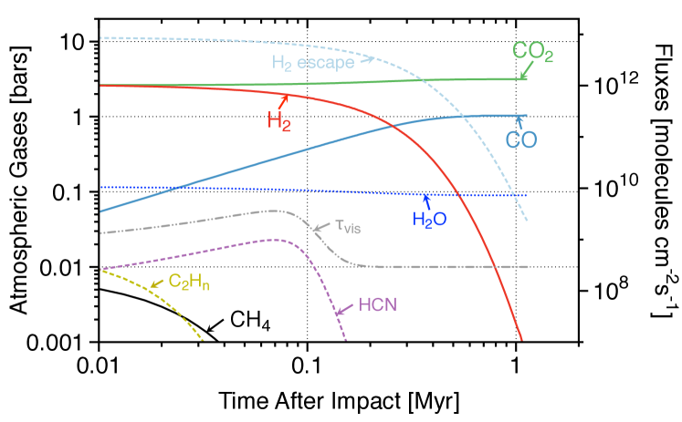
Figure 12: A non-ocean vaporizing impact. This case assumes 5 bars CO₂ and 1 bar of N₂ before the impact. Quenching is determined by gas phase reactions. Partial pressures (solid curves) are plotted against the left-hand axis, while fluxes (dashed curves) are plotted against the right-hand axis. Note the prolonged production of HCN in clear skies.

The first example, Figure 12, uses only the free Fe of the impact to reduce water and CO₂. This case assumes 5 bars CO₂ and 1 bar of N₂ in the atmosphere and 1.85 oceans of water on the surface before the impact. The impact evaporates about half the ocean, leaving deep waters less disturbed and some subsurface environments continuously habitable.

The atmosphere immediately after the impact holds 6.2 bars, mostly of H₂ and CO₂. This evolves after hydrogen escape into a 5.4 bar CO₂-N₂-CO atmosphere, with about 1 bar of CO left at the end of the simulation. For a short time the atmosphere provides a modest source of nitriles (comparable to modern Titan), but the cumulative production of organic material over the course of the event is equivalent to just 1 mm of precipitate. Unlike many of the cases we consider, the results are independent of stratospheric H₂O, because CO₂ is the oxidant. The H₂ from 15 meters of water escapes.

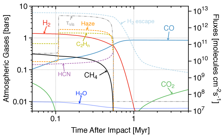
Figure 13: A non-ocean vaporizing impact that assumes that the atmosphere and ocean equilibrate with the relatively oxidizing QFM buffer at 650 K (i.e., at water’s critical temperature). Quenching is not determined by gas phase reactions. This case assumes 2 bars of CO₂ and 1 bar of N₂ before the impact. Shown are partial pressures.

The alternative sub-Vesta case (Figure 13) begins with the scenario presented in Figure 5 above, in which the atmosphere and ocean equilibrate with the QFM buffer at the critical temperature of 650 K. As in Figure 5, we assume that before the impact the atmosphere held 2 bars of CO₂ and one of N₂. The low equilibration temperature favors methane and ammonia, which are both rather abundant in a 2.3 bar atmosphere volumetrically dominated by 1.5 bars of H₂ (see Table 1), although most of the mass is in CH₄, CO₂, and N₂. For the photochemical evolution we assume a dry stratosphere ($0.1$ ppm H₂O).

The story told in Figure 13 is eventful. At first the atmosphere still holds enough CO₂ to be weakly oxidizing and organic production is modest, but after the CO₂ is gone stratospheric conditions become much more reduced, and organic production becomes considerable and stays so for about 0.5 Myrs. This second phase ends abruptly when the methane disappears. Cumulative production of organics is in the range of 2.5-5 m of hydrocarbons and nitriles. The H₂ from 40 meters of water escapes. The asymptotic state features about a bar of N₂ and CO each, the latter slowly oxidizing to CO₂ on geologic time scales.

5 Discussion

Benner et al. (2019a) have suggested that the greatest of the late veneer impacts (corresponding to those we simulate in Section 4.2.3) created a transiently reducing surface environment on Earth ca. 4.35 Ga and that this environment lasted for about 15 million years. They also suggest that the origin of the RNA world dates to this interval. They emphasized the difficulty in generating the simple N-rich organic molecules like cyanoacetylene and cyanamide needed to make purines and pyrimidines by paths other than highly reducing atmospheric chemistry. Although the dates and timing of events are less certain than Benner et al. (2019a) seem to suggest, in broad brush we find ourselves in general agreement. The quantity of reducing power is determined from the excess HSEs in the mantle. The timescale is set by the EUV radiation emitted by the young Sun. With due allowance for the uncertainty in both, a time scale in the general range of 10-100 Myrs is obtained by simply dividing the one quantity by the other, and it cannot be hugely wrong. As to when these events took place, opinions can differ, depending on how much weight one places on the ability of zircons to record the evolving conditions at the Earth’s surface (Carlson et al., 2014).

A possible problem posed by the biggest impact is that, although it brings the most reducing power, it is also the most likely to leave the surface too hot to promote prebiotic evolution, and for a long time. Even ignoring CO₂ and CH₄, the greenhouse effect provided by tens of bars of H₂ could raise the surface temperature to 400 K or more. Adding CO₂ or CH₄ or other greenhouse gases would make the surface still hotter. Impacts that are 10- to 100-fold smaller may therefore seem preferable, as these are more likely to leave the surface in a temperate state, albeit the reducing conditions do not last as long as for the bigger events. In a more recent study, Benner et al. (2019b) concede the potential advantages of less enormous impacts, while making a new point: the transience of highly-reduced impact-generated atmospheres lets the prebiotic system exploit other chemical pathways pertinent to the RNA world that work better in weakly-reduced (QFM mantle-derived) atmospheres. These make use of volcanic SO₂ (S in a deeply reduced atmosphere would be in H₂S), borates, and even the highly oxidized Mo⁺⁶.

An important opportunity that we have not quantitatively addressed is the delayed oxidation of impactor metallic iron that escaped immediate oxidation by the ocean or atmosphere. This iron would instead have been oxidized by recycled surface volatiles over the course of geologic time, which may have been millions or many tens of millions of years. If the chief oxidant were water, the chief volcanic gas would have been H₂. But if the chief oxidant were CO₂ (probably in the form of subducted carbonate), volcanic gases could have included significant amounts of the much more useful CH₄. Methane abundances are sensitive to pressure, but to give a specific example, CH₄ becomes the most abundant C-containing gas at the QFI buffer at 1400 K under 300 bars pressure, and it is still 10% at 1600 K. In the latter regime — one in which CO₂ must have been abundant in the atmosphere (else no carbonate) and CH₄ was abundant in undersea volcanic gases — the chief photochemical products would have been HCN and small organic acids, aldehydes, and carbonyls. This regime could have lasted for a long time, possibly tens of millions years or more.

5.1 Ammonia

Large impacts can generate considerable amounts of ammonia from hot H₂ and N₂. Ammonia’s fate involves many processes that are more complex than what we have been considering in this study. Nonetheless the inherent interest of ammonia as a constituent of the prebiotic environment is great enough that we will risk some speculations.

Ammonia is highly susceptible to UV photolysis at $185<\lambda<215$ nm, where its cross section is of the order of $3\times 10^{-18}$ cm², at wavelengths where the solar photon flux is much higher than at the shorter wavelengths where H₂O and CO₂ absorb. The products are NH and NH₂ radicals (Huebner et al., 1992) that swiftly react with each other, with oxygen, or with hydrogen in a series of reactions that efficiently recombine N₂ (Kuhn and Atreya, 1979). Without the protection of high altitude UV absorbers, a bar of NH₃ would revert to N₂ in less than $10^{4}$ years on early Earth.

However, if the atmosphere were also CH₄-dominated, as it likely would be were NH₃ abundant, the resulting hydrocarbon hazes might provide UV protection (Sagan and Chyba, 1997). Perhaps more important is that a significant fraction of the NH and NH₂ radicals that photolysis creates will have good odds of reacting with hydrocarbons to make amines and nitriles. Under these conditions the coupled hydrocarbon-ammonia photochemistry would lead to amines and nitriles (Miller, 1953).

The other factor to consider with ammonia is that it is very soluble in cool water and hence likely to rain out and partition into the ocean. The Henry’s Law coefficent for NH₃ in water is $K_{H}=4.6\times 10^{-5}e^{-4200/T}$ moles liter^-1 atm^-1. Much of the dissolved NH₃ hydrolyzes to ammonium, $\mathrm{NH}_{4}^{+}$. Ammonium abundance is related to NH₃(aq) and $pH$ by

$$\left[\mathrm{NH}_{4}^{+}\right]\left[\mathrm{OH}^{-}\right]=K_{b}\left[\mathrm{NH}_{3}\right]$$ (51)

in which the base constant $K_{b}$ is a weak function of temperature (Read, 1982),

$$\log{\left(K_{b}\right)}\approx-4.75-2.5\times 10^{-5}\left(T-298\right).$$ (52)

Expressing $\left[\mathrm{OH}^{-}\right]$ in terms of $pH$ and the auto-ionization constant $K_{w}$ of water (which can be crudely approximated as a function of $T$ by $\log{\left(K_{w}\right)}=-14+0.03\left(T-298\right)-7.5\times 10^{-5}\left(T-298\right)^{2}$), the ammonium/ammonia ratio is

$$\log{\left\{\left[\mathrm{NH}_{4}^{+}\right]/\left[\mathrm{NH}_{3}\right]\right\}}=\log{\left(K_{b}\right)}-\log{\left(K_{w}\right)}-\log{\left(pH\right)}.$$ (53)

If all the nitrogen currently in Earth’s atmosphere were converted to NH₃, the equilibrium NH₃ gas pressure above an ocean with $pH$ of 7.8 and temperature 298 K would be just 100 mbars (yet enough to generate a considerable greenhouse effect). The other 1.56 bars of N would be dissolved in the oceans, 97% as NH${}_{4}^{+}$.

Hotter oceans are interesting. At 373 K, other things equal, the $\mathrm{NH}_{4}^{+}/\mathrm{NH}_{3}$ ratio would drop to $\sim 2$. The equilibrium NH₃ gas pressure over the ocean would be 0.02 bars. The other 1.54 bars of NH₃ would be in the oceans, divided between NH${}_{4}^{+}$ and NH₃. At 500 K the $pH$ would be another unit lower, and NH${}_{4}^{+}$ less abundant than NH₃. The equilibrium NH₃ gas pressure in the atmosphere rises to 0.7-1.0 bar, with the rest of the N divided between NH₃ and NH${}_{4}^{+}$ dissolved in the ocean. In this case the ammonia would probably be photochemically destroyed very quickly, although many of the products would be prebiotically interesting if CH₄ were also abundant.

This exercise suggests that NH₃ would last longest as ammonium ions in cold seas under an organic haze, conditions rather similar to those sometimes imagined for early Titan (Lorenz and Mitton, 2002). We speculate that ammonia’s powerful greenhouse effect can lead to a strong positive feedback between ocean temperature and exsolution that would in turn speed ammonia’s photochemical destruction. It is not obvious that keeping ammonia around for a long time is a better option for prebiotic purposes than a rapid dump of a wide variety of nitrogenous products into warm oceans. Here we simply present these cases as end-members.

5.2 The Hadean impact cascade

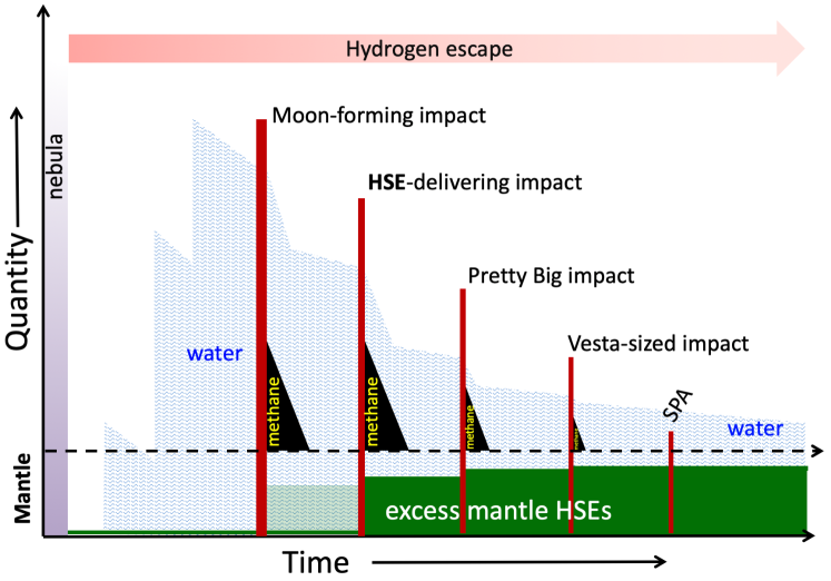
Figure 14: A schematic history of water, methane, and highly siderophile elements on Earth in response to late great impacts. “SPA” refers to an impact on the scale of the one that excavated the lunar S. Pole-Aitken basin — too small to evaporate the oceans — which is implied here by submerging SPA’s pole under the waves. Major impacts are shown decreasing in magnitude as time passed, but the true order leaves much to chance; it is possible that the largest of the ocean-vaporizers was also the last.

Figure 14 presents a notional history of water, methane, and highly siderophile elements (HSEs) on early Earth in response to late great impacts. The last stage of this impact history is evident on the face of the Moon and is often called the “late heavy bombardment,” often referred to as the “LHB.” Water on Earth probably accreted before the Moon-forming impact, and the quantity of water on Earth was likely to have decreased during the late accretion of what the isotopic evidence shows were mostly water-poor bodies. Transient methane-rich atmospheres are generated by ocean-vaporizing impacts. Here we presume that the mantle’s excess HSEs were delivered mostly by a single impact, with light shading indicating an allowance for the HSEs dating to the Moon-forming impact itself. Major impacts are shown decreasing in magnitude as time passed, but the true order leaves much to chance; it is possible that the largest of the ocean-vaporizers was also the last. Each great impact left Earth in a state resembling somewhat the state of early Earth as sketched by Urey (1952) for periods that may have been less than a million years or as long as 100 million years, the duration depending on the size of the impact and on the flux of ultraviolet radiation from the young Sun.

6 Conclusions

Great impacts of Earth’s late accretion — especially those that evaporated the oceans — differ from lesser impacts in several important ways. First, they delivered significant reducing power in the form of metallic iron to Earth’s surface environments. We infer this because the characteristic isotopic fingerprints of the mantle’s highly siderophile elements (HSEs) establishes the late veneer as kin to the enstatite chondrites, aubrites, and type IAB iron meteorites, all of which are profoundly reduced and bear ample metallic iron. The iron was oxidized in the crust or mantle, which we know because the HSEs are unfractionated, and hence there was no significant loss of metal to the core. Water and CO₂ were the plausible oxidants; hence hydrogen, carbon monoxide, and methane were the plausible products. Second, the high H₂O and H₂ vapor pressures in a reduced steam atmosphere favor CH₄ and NH₃ over CO or N₂, a preference that goes as the square of the pressure. Third, cooling after impact was slow because the thermal inertia of a hot steam atmosphere containing hundreds of bars of gas is large. It takes more than a thousand years to cool 270 bars (an ocean) of steam at the runaway greenhouse cooling rate. The result is that quench temperatures for gas phase reactions in the CH₄-CO-CO₂-H₂O-H₂ system drop to $\sim$800 K or less, and quench temperatures for the NH₃-N₂-H₂O-H₂ system drop to $\sim$1100 K, and hence both methane and ammonia form directly by gas phase reactions.

How much methane actually forms depends on how much carbon was available to the atmosphere before the impact, on how much reducing power was delivered by the impact, how much of the delivered iron reacts with the atmosphere and ocean as opposed to being deeply buried under the ejecta, and on whether catalysts were active to reduce the quench temperature still further. In addition to atmospheric CO₂ and CO, available carbon inventories would include any CO₂ dissolved in the oceans, and any CO₂ in carbonate rocks that were not buried too deeply to be liberated by shock-heating. Methane production could have been enormous. If for example we presume that a maximum-late-veneer scale impact took place on an Earth with a 100 bar of CO₂ atmosphere (perhaps left over from the Moon-forming impact, Zahnle et al., 2007), and 5 km of water at the surface, there is enough time and reducing power to convert all of the carbon to methane, diluted in several tens of bars of H₂. The resulting atmosphere is rather Neptune-like, with a scale height in the range of 50-100 km.

Another interesting aspect of the biggest impacts is that much of the delivered iron may have been too deeply buried in the ejecta blanket to be oxidized in the first thousands of years after the impact. Under these circumstances the iron must have been oxidized on a longer time scale set by broadly geological processes that govern the interchange of surface volatiles with crustal and mantle materials. Although we have not presented models of such a scenario here, we can expect that gases emitted from a mantle with extant metallic iron would be strongly reduced over an extended period of time. How important this impact coda might be to the origin of life depends on whether these gases included methane.

Earth’s hydrogen-methane atmospheres would have been physically stable — they did not blow off — but they were subject to photochemical dissipation, as both hydrogen escape and methane photolysis are effectively irreversible. The rate the atmosphere evolves is set by the flux of solar far and extreme ultraviolet radiations. Here we use a zero-D photochemical model to simulate atmospheric evolution: we count the photons and apportion their effects. We find that the biggest late veneer impacts can generate (cumulatively) as much as 500 meters of organic over tens of millions of years, while smaller impacts do commensurately less in commensurately less time.

The details of atmospheric evolution of the transient reduced atmosphere are mostly determined by quantities (i.e., bigger impacts have bigger impacts), but there is one ill-constrained modeling parameter — the stratospheric water vapor mixing ratio — to which the outcomes are sensitive. Moister stratospheres are relatively oxidizing, while drier stratospheres are profoundly reducing and resemble conditions on modern Titan, but sped up by a factor of 1000. We see a sharp transition in photochemical products determined by the competition between oxidation and reduction. In our models, the transition appears to take place at stratosphere H₂O mixing ratios in the range of 0.1-1 ppm, moisture levels that are not very different from Earth today. A more sophisticated model might predict a smoother transition, or a different critical water abundance for a sharp transition.

Lesser impacts are of course less impactful. Tens of smaller, non-ocean-vaporizing impacts will generate significant amounts of H₂ and CO but very little CH₄ or NH₃ unless catalysts were available to reduce the quench temperature. Hydrogen and CO are useful ingredients for a bootstrapping origin of life scenario in which the biochemical evolution began by catalyzing the kinds of chemical reactions that build hydrocarbons from CO and H₂. But if the primary requirements for life are methane, ammonia, HCN, and their photochemical derivatives, only the biggest impacts or as-yet-unknown chemistry will do.

From the points of view of the origin of life and biblical metaphors, the great impacts may be double-edged swords. In their aftermath they leave Earth primed and ready to start life under a classic Urey-Miller H₂-rich, CH₄-rich, possibly even NH₃-rich atmosphere that origin of life theorists have long favored. Unfortunately, at least with the biggest of them, the first act is an attempt to wipe out everything that had been accomplished before. What this suggests is that impact-generated transient atmospheres may give a planet only one highly favorable roll of the dice. Smaller, less dangerous impacts can inject significant amounts of new H₂ or CO into the system that might be capable of building on previous progress, but these smaller impacts require unidentified catalysts or unidentified chemistry to generate large amounts of CH₄ or NH₃. And even if all such conditions were met, there could not have many such impacts, probably no more than a dozen.

7 Acknowledgements

This work was in part supported by the NASA Exobiology Program, grant 80NSSC18K1082. DCC was supported by the Simons Foundation. We thank Y. Abe, S. Benner, R. Carlson, S. Desch, B. Fegley Jr., V.S. Meadows, A. O’Keefe, L. Schaefer, N.H. Sleep, J.H. Waite.

Appendix A: Mineral buffers, three of them

We give three representative mineral buffers here. The quartz-fayalite-iron (QFI) buffer is the most reduced buffer we consider

$$2{\rm Fe}+{\rm SiO}_{2}+{\rm O}_{2}\leftrightarrow{\rm Fe}_{2}{\rm SiO}_{4}.$$ (R6)

The oxygen fugacity of the QFI buffer is approximated by

$$f_{\mathrm{O}_{2}}=1.962\times 10^{-6}T^{3.443}\exp{\left(-54573/T-2.073\times 10^{5}/T^{1.5}\right)}.$$ (54)

Curve fits are based on literature fits for temperatures between $900\!<\!T\!<\!1420$ K from O’Neill and Eggins 2002. The QFI buffer is representative of many chondritic meteorites (Schaefer and Fegley, 2017).

The iron-wüstite buffer (IW) is based on a simple reaction

$${\rm Fe}+{1\over 2}{\rm O}_{2}\leftrightarrow{\rm FeO}.$$ (R7)

The oxygen fugacity of the IW buffer is approximated by

$$f_{\mathrm{O}_{2}}=3.1924\times 10^{-6}T^{2.4952}\exp{\left(-39461/T-3.221\times 10^{5}/T^{1.5}\right)}$$ (55)

The direct reaction of water with iron to make FeO and H₂ seems kinetically straightforward and hence the IW buffer seems appropriate for the interaction of hot iron and water.

The fayalite-magnetite-quartz buffer (abbreviated FMQ or QFM) is representative of modern volcanic degassing and is regarded as typical of the modern Earth’s mantle. It is the most oxidized mineral buffer that we consider. The generic QFM reaction is

$$3{\rm Fe}_{2}{\rm SiO}_{4}+{\rm O}_{2}\leftrightarrow 2{\rm Fe}_{3}{\rm O}_{4}+3{\rm SiO}_{2}.$$ (R8)

The oxygen fugacity of the QFM buffer can be approximated by

$$f_{\mathrm{O}_{2}}=3.015\times 10^{-4}T^{3.449}\exp{\left(-53649/T\right)}.$$ (56)

Oxygen fugacity $f_{\mathrm{O}_{2}}$ has units of atmospheres — we treat $f_{\mathrm{O}_{2}}$ as effectively the same as the O₂ partial pressure $p{\mathrm{O}_{2}}$.

Appendix B. Chemical reactions discussed in text

Reaction				rate at 298 K cm3 s-1
R11	$\mathrm{N}(^{2}\mathrm{D})+\mathrm{H}_{2}$	$\rightarrow$	$\mathrm{NH}+\mathrm{H}$	$k_{11}=2.2\times 10^{-12}$
R12	$\mathrm{N}(^{2}\mathrm{D})+\mathrm{CH}_{4}$	$\rightarrow$	products	$k_{12}=4\times 10^{-12}$
		$\rightarrow$	$\mathrm{H}_{2}\mathrm{CNH}+\mathrm{H}$	$k_{12a}=0.75\times k_{12}$
		$\rightarrow$	$\mathrm{NH}+\mathrm{CH}_{3}$	$k_{12b}=0.25\times k_{12}$
R13	$\mathrm{N}(^{2}\mathrm{D})+\mathrm{H}_{2}\mathrm{O}$	$\rightarrow$	productsa	$k_{13}=5\times 10^{-11}$
R14	$\mathrm{N}(^{2}\mathrm{D})+\mathrm{CO}_{2}$	$\rightarrow$	$\mathrm{NO}+\mathrm{CO}$	$k_{14}=3.6\times 10^{-13}$
R15	$\mathrm{N}(^{2}\mathrm{D})+\mathrm{CO}$	$\rightarrow$	$\mathrm{N}+\mathrm{CO}$	$k_{15}=1.9\times 10^{-12}$
R16	$\mathrm{N}(^{2}\mathrm{D})+\mathrm{N}_{2}$	$\rightarrow$	$\mathrm{N}+\mathrm{N}_{2}$	$k_{16}=1.7\times 10^{-14}$
R21	$\mathrm{O}(^{1}\mathrm{D})+\mathrm{H}_{2}$	$\rightarrow$	$\mathrm{OH}+\mathrm{H}$	$k_{21}=1.1\times 10^{-10}$
R22	$\mathrm{O}(^{1}\mathrm{D})+\mathrm{CH}_{4}$	$\rightarrow$	products	$k_{22}=1.5\times 10^{-10}$
		$\rightarrow$	$\mathrm{H}_{2}\mathrm{COH}+\mathrm{H}$	$k_{22a}=0.1\times k_{22}$
		$\rightarrow$	$\mathrm{OH}+\mathrm{CH}_{3}$	$k_{22b}=0.9\times k_{22}$
R23	$\mathrm{O}(^{1}\mathrm{D})+\mathrm{H}_{2}\mathrm{O}$	$\rightarrow$	$\mathrm{OH}+\mathrm{OH}$	$k_{23}=2.2\times 10^{-10}$
R24	$\mathrm{O}(^{1}\mathrm{D})+\mathrm{CO}_{2}$	$\rightarrow$	$\mathrm{O}+\mathrm{CO}_{2}$	$k_{24}=7.4\times 10^{-11}$
R25	$\mathrm{O}(^{1}\mathrm{D})+\mathrm{CO}$	$\rightarrow$	$\mathrm{O}+\mathrm{CO}$	$k_{25}=7\times 10^{-11}$
R26	$\mathrm{O}(^{1}\mathrm{D})+\mathrm{N}_{2}$	$\rightarrow$	$\mathrm{O}+\mathrm{N}_{2}$	$k_{26}=1.8\times 10^{-11}$
R31	$\mathrm{OH}+\mathrm{H}_{2}$	$\rightarrow$	$\mathrm{H}+\mathrm{H}_{2}\mathrm{O}$	$k_{31}=6\times 10^{-15}$
R32	$\mathrm{OH}+\mathrm{CH}_{4}$	$\rightarrow$	$\mathrm{CH}_{3}+\mathrm{H}_{2}\mathrm{O}$	$k_{32}=6\times 10^{-15}$
R35	$\mathrm{OH}+\mathrm{CO}$	$\rightarrow$	$\mathrm{CO}_{2}+\mathrm{H}$	$k_{35}=1.2\times 10^{-13}$
R37	$\mathrm{OH}+\mathrm{CH}_{2}$	$\rightarrow$	$\mathrm{H}_{2}\mathrm{CO}+\mathrm{H}$	$k_{37}=1.2\times 10^{-10}$
R38	$\mathrm{OH}+\mathrm{CH}_{3}$	$\rightarrow$	products	$k_{38}=6\times 10^{-11}$
R41	$\mathrm{O}+\mathrm{H}_{2}$	$\rightarrow$	$\mathrm{H}+\mathrm{OH}$	$k_{41}=1\times 10^{-17}$
R42	$\mathrm{O}+\mathrm{CH}_{4}$	$\rightarrow$	$\mathrm{CH}_{3}+\mathrm{OH}$	$k_{42}=7\times 10^{-18}$
R45	$\mathrm{O}+\mathrm{CO}$	$\rightarrow$	$\mathrm{CO}_{2}$	$k_{45}^{b}=4.0\times 10^{-17}$
R47	$\mathrm{O}+\mathrm{CH}_{2}$	$\rightarrow$	$\mathrm{HCO}+\mathrm{H}$	$k_{47}=1.2\times 10^{-10}$
R48	$\mathrm{O}+\mathrm{CH}_{3}$	$\rightarrow$	$\mathrm{H}_{2}\mathrm{CO}+\mathrm{H}$	$k_{48}=1.2\times 10^{-10}$
R57	$\mathrm{N}+\mathrm{CH}_{2}$	$\rightarrow$	$\mathrm{HCN}+\mathrm{H}$	$k_{57}=1.2\times 10^{-10}$
R58	$\mathrm{N}+\mathrm{CH}_{3}$	$\rightarrow$	$\mathrm{H}_{2}\mathrm{CN}+\mathrm{H}$	$k_{58}=1.1\times 10^{-10}$
R78	$\mathrm{CH}_{2}+\mathrm{CH}_{3}$	$\rightarrow$	$\mathrm{C}_{2}\mathrm{H}_{4}+\mathrm{H}$	$k_{78}=7\times 10^{-11}$
$a$ - Products are plausibly HNO and H.
$b$ - High pressure limit

Appendix C. Photoionization

Photoionizing photons (EUV₁ and $S_{1}$ in Table 2) are important for hydrogen escape but less important than photolysis for chemistry. To first approximation, CO and N₂ usually survive photoionization intact by charge exchange. Photoionization of CO₂ usually creates CO${}^{+}_{2}$ ions, which can dissociate to CO after reaction with atomic H or O, and can charge exchange with CH₄ to make CH${}_{4}^{+}$, leaving CO₂ intact while ultimately disintegrating CH₄. As we are not tracking H or O, we arbitrarily assume that 20% of CO₂ photoionizations generate CO.

$$\left({dN_{\mathrm{CO}_{2}}\over dt}\right)_{\!\!ions}=-0.2\Phi_{\mathrm{CO}_{2}}^{\ast}$$ (57)

Photoionization of water usually yields H₂O⁺, which reacts with H₂ to make H₃O⁺ and H; with CH₄ to make H₃O⁺ and CH₃; and with CO to make HCO⁺ and OH. Both H₃O⁺ and HCO⁺ dissociatively recombine. The $\mathrm{H}_{2}\mathrm{O}^{+}+\mathrm{CH}_{4}$ channel counts as a loss for CH₄, while the HCO⁺ channel counts as a source of OH. For cases of most interest to us here, H₂O will be condensed at the surface and will not be a major constituent at the top of the atmosphere, the H₂O photoionization terms will be small.

The chief chemical consequence of photo-ionization is that CH₄ is broken down into reactive CH_n radicals. Direct photo-ionization mostly yields CH${}_{4}^{+}$ or CH${}_{3}^{+}$, which in subsequent reactions are almost guaranteed to lead to the loss CH₄. The other molecular ions also react with CH₄, sparking chains of reactions that lead to CH_n radicals. E.g., N${}_{2}^{+}$ can exchange with CO to make CO⁺, CO⁺ can exchange with CO₂ to make CO${}_{2}^{+}$, CO${}_{2}^{+}$ can react with CH₄ to free CH_n radicals. The net

$$\left({dN_{\mathrm{CH}_{4}}\over dt}\right)_{\!\!ions}=-\Phi_{\mathrm{CH}_{4}}^{\!\ast}-\Phi_{\mathrm{H}_{2}}^{\!\ast}{N_{\mathrm{CH}_{4}}\over X_{1}}-\Phi_{\mathrm{CO}_{2}}^{\!\ast}{N_{\mathrm{CH}_{4}}\over X_{3}}-\Phi_{\mathrm{CO}}^{\!\ast}\left({N_{\mathrm{CH}_{4}}\over X_{2}}+{N_{\mathrm{CO}_{2}}\over X_{2}}{N_{\mathrm{CH}_{4}}\over X_{3}}\right)$$

$$-\Phi_{\mathrm{N}_{2}}^{\!\ast}\left({N_{\mathrm{CH}_{4}}\over X_{1}}+{N_{\mathrm{CO}}\over X_{1}}{N_{\mathrm{CH}_{4}}\over X_{2}}+{N_{\mathrm{CO}}\over X_{1}}{N_{\mathrm{CO}_{2}}\over X_{2}}{N_{\mathrm{CH}_{4}}\over X_{3}}+{N_{\mathrm{H}_{2}\mathrm{O}}\over X_{1}}{N_{\mathrm{CH}_{4}}\over X_{4}}\right)-\Phi_{\mathrm{H}_{2}\mathrm{O}}^{\!\ast}{N_{\mathrm{CH}_{4}}\over X_{4}}$$ (58)

where the $X_{k}$ factors crudely account for the branching patterns in the ion cascades:

$$X_{1} = N_{\mathrm{H}_{2}}+N_{\mathrm{CH}_{4}}+N_{\mathrm{H}_{2}\mathrm{O}}+N_{\mathrm{CO}}+N_{\mathrm{CO}_{2}}$$ (59)

$$X_{2} = N_{\mathrm{CH}_{4}}+N_{\mathrm{H}_{2}\mathrm{O}}+N_{\mathrm{CO}_{2}}$$ (60)

$$X_{3} = N_{\mathrm{H}_{2}}+N_{\mathrm{CH}_{4}}+N_{\mathrm{H}_{2}\mathrm{O}}$$ (61)

$$X_{4} = N_{\mathrm{H}_{2}}+N_{\mathrm{CH}_{4}}$$ (62)

Equation 58 represents about 20% of total CH₄ photolysis.

References

- Abe (1997) Abe, Y., 1997. Thermal and chemical evolution of the terrestrial magma ocean. Phys. Earth Planet. Int. 100, 27-39.
- Abe and Matsui (1988) Abe, Y., Matsui, T., 1988. Evolution of an impact-generated H2O-CO2 atmosphere and formation of a hot proto-ocean on Earth. J. Atmos. Sci. 45, 3081–3101.
- Abelson (1966) Abelson PH (1966) Chemical Events on the Primitive Earth. Proc. Nat. Acad. Sci. 55, 1365-1372.
- Agnor and Asphaug (2004) Agnor CB, Asphaug E (2004). Accretion Efficiency during Planetary Collisions. Astrophys. J. 613, L157-L160
- Ahrens et al. (1989) Ahrens TJ, O’Keefe JD, Lange MA (1989). Formation of atmospheres during accretion of the terrestrial planets. In Origin and Evolution of Planetary and Satellite Atmospheres. Atreya SK, Pollack JB, and Matthews MS (Eds), University of Arizona Press, pp. 328-385.
- Albarède et al. (2013) Albarède F, Ballhaus C, Blichert-Toft J, Lee C-T, Marty B, Moynier F, Yin Q-Z (2013). Asteroidal impacts and the origin of terrestrial and lunar volatiles. Icarus 222, 44-52.
- Alexander (2017) Alexander CMO’D (2017). The origin of inner Solar System water. Phil. Trans. Roy. Soc. A, 375, id.20150384.
- Anders (1989) Anders E (1989). Pre-biotic organic matter from comets and asteroids. Nature 342, 255-257.
- Anders and Owen (1977) Anders E, Owen T (1977). Mars and earth - Origin and abundance of volatiles. Science 198, 453-465.
- Anicich (1993) Anicich, V.G. (1993). A survey of bimolecular ion-molecule reactions for use in modeling the chemistry of planetary atmospheres, cometary comae, and interstellar clouds. Astrophys. J. Supp. 84, 215-315.
- Asphaug et al. (2006) Asphaug E., Agnor C., Williams Q. (2006). Hit-and-run planetary collisions. Nature 439, 155-160.
- Armstrong et al. (2019) Armstrong K, Frost DJ, McCammon CA, Rubie DC, Ballaran TB (2019). Deep magma ocean formation set the oxidation state of Earth’s mantle. Science 365, 903-906.
- Aulbach and Stagno (2016) Aulbach S, Stagno V (2016). Evidence for a reducing Archean ambient mantle and its effects on the carbon cycle. Geology 44,751-754.
- Aulbach et al. (2017) Aulbach S. Woodland A. B. Vasilyev P. Galvez M. E. Viljoen K. S. (2017). Effects of low-pressure igneous processes and subduction on FeFe and redox state of mantle eclogites from Lace (Kaapvaal craton). Earth Planet. Sci. Lett. 474, 283-295.
- Benner et al. (2019a) Benner SA, Bell EA, Biondi E, Brasser R, Carell T,Kim H-J, Mojzsis SJ, Omran A, Pasek MA, Trail D (2019). When did Life Likely Emerge on Earth in an RNA-First Process? ChemSystChem doi:10.1002/syst.201900035
- Benner et al. (2019b) Benner SA, Kim HJ, Biondi E. (2019). Prebiotic Chemistry that Could Not Not Have Happened. Life 9, 84 (16 pp.). doi:10.3390/life9040084
- Bermingham et al. (2018) Bermingham K.R., Worsham E.A., Walker R.J. (2018). New insights into Mo and Ru isotope variation in the nebula and terrestrial planet accretionary genetics. Earth Planet. Sci. Lett. 487, 221-229.
- Bottke et al. (2010) Bottke W.F., Walker R.J., Day J.M.D., Nesvorny D., Elkins-Tanton L. (2010). Stochastic late accretion to Earth, the Moon, and Mars. Science 330, 1527-1530.
- Brasser et al. (2016) Brasser R., Mojzsis S.J., Werner S.C., Matsumura S., Ida S. (2016). Late veneer and late accretion to the terrestrial planets. Earth Planet. Sci. Lett. 455, 85-93.
- Budde et al. (2019) Budde G, Burkhardt C, Kleine T (2019). Molybdenum isotopic evidence for the late accretion of outer Solar System material to Earth. Nature Astron. 3, 736-741.
- Burkhardt et al. (2019) Burkhardt C, Dauphas N, Hans U, Bourdon B, Kleine T (2019). Elemental and isotopic variability in solar system materials by mixing and processing of primordial disk reservoirs. Geochim. Cosmochim. Acta 261, 145-170.
- Canil (2002) Canil D (2002). Vanadium in peridotites, mantle redox and tectonic environments: Archean to present. Earth Planetary Science Letters 195, 75-90.
- Carlson et al. (2014) Carlson RW, Garnero E, Harrison TM, Li J, Manga M, McDonough WF, Mukhopadhyay S, Romanowicz B, Rubie D, Williams Q, Zhong S (2014). How Did Early Earth Become Our Modern World? Annual Rev. Earth Planet. Sci. 42, 51-178.
- Carlson et al. (2018) Carlson RW, Brasser R, Yin Q-Z, Fischer-Gödde M, Qin L (2018). Feedstocks of the Terrestrial Planets. Book chapter. Before the Moon
- Chase (1998) Chase MW (1998). NIST-JANAF Thermochemical Tables, Fourth Edition. J. Phys. Chem. Ref. Data Monograph 9, 1-1951.
- Choudhry et al. (2014) Choudhry KI, Carvajal-Ortiz RA, Kallikragas DT, Svishchev IM (2014). Hydrogen evolution rate during the corrosion of stainless steel in supercritical water. Corrosion Science 83, 226-233.
- Chyba and Sagan (1992) Chyba CF, Sagan C (1992). Endogenous production, exogenous delivery and impact-shock synthesis of organic molecules: an inventory for the origins of life. Nature 355, 125-132.
- Claire et al. (2012) Claire MW, Sheets J, Cohen M, Ribas I., Meadows VS, Catling DC (2012). The evolution of solar flux from 0.1 nm to 160 m: Quantitative estimates for planetary studies. Astrophys. J. 757, 95.
- Cleaves et al. (2008) Cleaves HJ, Chalmers JH, Lazcano A, Miller SL, Bada JL. (2008) A reassessment of prebiotic organic synthesis in neutral planetary atmospheres. Orig Life Evol Biosph. 38, 105-1156.
- Curdt et al. (2001) Curdt W, Brekke P, Feldman U, Wilhelm K, Dwivedi BN, Schüle U, Lemaire P (2001). The SUMER spectral atlas of solar disk features. Astron. Astrophys.
- Dauphas (2017) Dauphas N. (2017). The isotopic nature of the Earth’s accreting material through time. Nature 541, 521-524.
- Dauphas and Morbidelli (2014) Dauphas N., Morbidelli A. (2014). Geochemical and Planetary Dynamical Views on the Origin of Earth’s Atmosphere and Oceans. Treatise in Geochemistry 2nd Edition http://dx.doi.org/10.1016/B978-0-08-095975-7.01301-2
- Day et al. (2016) Day JMD, Brandon AD, Walker RJ (2016). Highly siderophile elements in Earth, Mars, the Moon, and Asteroids. Rev. Minerology Geochem. 81, 161-238.
- Dean and Bozzelli (2000) Dean AM, Bozzelli JW (2000). Combustion chemistry of nitrogen. In Gas-Phase Combustion Chemistry, WC Gardiner Jr (Ed), Springer, pp. 125-341.
- Delano (2001) Delano JW (2001). Redox history of the Earth’s interior since approximately 3900 Ma: implications for prebiotic molecules. Origin Life Evol. Biosphere 31, 311-341.
- Dreibus and Wänke (1989) Dreibus, G., Wänke (1989). Supply and loss of volatile constituents during the accretion of the terrestrial planets. In Origin and Evolution of Planetary and Satellite Atmospheres, edited by S.K. Atreya, J.B. Pollack, M.S. Matthews, pp. 268-288, University of Arizona Press, Tucson.
- Elkins-Tanton and Seager (2008) Elkins-Tanton L, Seager S (2008). Ranges of Atmospheric Mass and Composition of Super-Earth Exoplanets. Astrophys. J. 685, 1237-1246.
- Elkins-Tanton (2008) Elkins-Tanton L. (2008). Linked magma ocean solidification and atmospheric growth for Earth and Mars. Earth Planet. Sci. Lett. 271, 181-191.
- Fegley and Prinn (1998) Chemical reprocessing of the Earth’s present and primordial atmosphere by large impacts. In The Barringer Lectures. Unpublished book.
- Ferris et al. (1978) Ferris JF, Joshi PC, Edelson EH, Lawless JG (1978). HCN: a plausible source of purines, pyrimidines and amino acids on the primitive Earth. J Mol Evol 11, 293-311
- Fischer-Gödde et al. (2015) Fischer-Gödde M., Burkhardt C, Kruijer TS, Kleine T. (2015). Ru isotope heterogeneity in the solar protoplanetary disk. Geochim. Cosmochim. Acta 168 151-171.
- Fischer-Gödde and Kleine (2017) Fischer-Gödde M., Kleine T. (2017). Ruthenium isotopic evidence for an inner Solar System origin of the late veneer. Nature 541, 525-527.
- Frost and McCammon (2008) Frost D.J., McCammon C.A. (2008). The redox state of Earth’s mantle. AnnuṘev. Earth Planet. Sci. 36, 389-420.
- Genda et al. (2017a) Genda H., Brasser R., Mojzsis S.J. (2017a). The terrestrial late veneer from core disruption of a lunar-sized impactor. Earth Planet. Sci. Lett. 480, 25-32.
- Genda et al. (2017b) Genda H, Iizuka T, Sasaki T, Ueno Y, Ikoma M (2017b). Ejection of iron-bearing giant-impact fragments and the dynamical and geochemical influence of the fragment re-accretion Earth Planet. Sci. Lett. 470, p. 87-95.
- Greenwood et al. (2018) Greenwood R.C., Barrat J-A, Miller MF, Anand M, NDauphas N, Franchi IA, Sillard P, Starkey NA (2018). Oxygen isotopic evidence for accretion of Earth’s water before a high-energy Moon-forming giant impact. Sci. Adv. 4, eaao5928 (8 pp.).
- Haldane (1929) Haldane JBS (1929). The Origin of Life. Rationalist Annual 1929, 12pp.
- Hashimoto et al. (2007) Hashimoto GL, Abe Y, and Seiji Sugita S (2007). The chemical composition of the early terrestrial atmosphere: Formation of a reducing atmosphere from CI-like material. J. Geophys. Res. 112, E05010, doi:10.1029/2006JE002844.
- Heays et al. (2014) Heays AN, Visser R, Gredel R, Ubachs W, Lewis BR, Gibson ST, van Dishoeck EF (2014). Isotope selective photodissociation of N2 by the interstellar radiation field and cosmic rays. Astron. Astrphys. 562, id.A61, 16 pp.
- Herron (1999) Herron JT (1999). Evaluated chemical kinetics data for reactions of N(2D), N(2P), and N2(A) in the gas phase. J. Phys. Chem. Ref. Data 28, 1453-1483.
- Hirschmann (2012) Hirschmann M. M. (2012). Magma ocean influence on early atmosphere mass and composition. Earth Planet. Sci. Lett. 341-344, 48-57.
- Hirschmann (2013) Hirschmann M. M. (2013). Fe-carbonyl is a key player in planetary magmas. Proc. Nat. Acad. Sci. 110, 7967-7968.
- Holland (1964) Holland HD (1964). On the chemical evolution of the terrestrial and cytherian atmospheres. In: Brancazio PJ, Cameron AGW (Eds.). The Origin and Evolution of Atmospheres and Oceans. John Wiley and Sons, New York, pp. 86-101.
- Holland (1984) Holland HD (1984). The Chemical Evolution of the Atmosphere and Oceans. Princeton University Press.
- Hopp and Kleine (2018) Hopp T., Kleine T. (2018). Nature of late accretion to Earth inferred from mass-dependent Ru isotopic compositions of chondrites and mantle peridotites. Earth Planet. Sci. Lett. 494, 50-59.
- Hörst et al. (2012) Hörst SM, Yelle RV, Buch A, Carrasco N, Cernogora G, Dutuit O, Quirico, E, Sciamma-O’Brien E, Smith MA, Somogyi Á, Szopa C, Thissen R, Vuitton V (2012). Formation of Amino Acids and Nucleotide Bases in a Titan Atmosphere Simulation Experiment. Astrobiology 12, 809-817.
- Hörst et al. (2018b) Hörst SM, He C, Ugelow MS, Jellinek AM, Pierrehumbert RT, Tolbert MA (2018). Exploring the Atmosphere of Neoproterozoic Earth: The Effect of O2 on Haze Formation and Composition. Astrophys. J. 858, article id. 119, 9 pp.
- Huebner et al. (1992) Huebner W. F., Keady J. J., Lyon S. P. (1992). Solar photo rates for planetary atmospheres and atmospheric pollutants. Astrophys. Space Sci. 195, 1-294.
- Johnson et al. (2008) Johnson AP, Cleaves HJ, Dworkin JP, Glavin DP, Lazcano A, and Jeffrey L. Bada JL (2008). The Miller volcanic spark discharge experiment. Science 322, 404.
- Kasting (1990) Kasting JF (1990). Bolide impacts and the oxidation state of carbon in the Earth’s early atmosphere. Origins of Life and Evolution of the Biosphere 20, 199-231.
- Kraus et al. (2015) Kraus RG, Root S, Lemke RW, Stewart ST, Jacobsen SB, Mattsson TR (2015). Impact vaporization of planetesimal cores in the late stages of planet formation. Nat. Geosci. 8, 269-272.
- Kress and McKay (2004) Kress ME and McKay CP (2004). Formation of methane in comet impacts: implications for Earth, Mars, and Titan. Icarus 168, 475-483.
- Kuhn and Atreya (1979) Kuhn WR, Atreya SK (1979). Ammonia photolysis and the greenhouse effect in the primordial atmosphere of the earth. Icarus 37, 207-213.
- Kuramoto (1997) Kuramoto K (1997). Accretion, core formation, H and C evolution of the Earth and Mars. Phys. Earth Planet. Int. 100, 3-20.
- Kuwahara and Sugita (2015) Kuwahara H., Sugita S. (2015). The molecular composition of impact-generated atmospheres on terrestrial planets during the post-accretion stage. Icarus 257, 290-301.
- Lasaga et al. (1971) Lasaga A.C, Holland H.D., Dwyer M.J. (1971). Primordial oil slick. Science 174, 53-55.
- Li et al. (2013) Li X, Heays AN, Visser R, Ubachs W, Lewis BR, Gibson ST, van Dishoeck EF (2013). Photodissociation of interstellar N2. Astron. Astrophys. 555, id.A14, 18 pp.
- Liang et al. (2007) Liang M-C, Heays AN, Lewis BR, Gibson ST, Yung YL (2007). Source of nitrogen isotope anomaly in HCN in the atmosphere of Titan. Astrophys. J. 664, L115-L118.
- Line et al. (2011) Line MR, Vasisht G, Chen P, Angerhausen D, Yung YL (2011). Thermochemical and photochemical kinetics in cooler hydrogen-dominated extrasolar planets: A methane-poor GJ436b? Astrophys. J. 738, 32 (14 pp.).
- Lodders and Fegley (1998) Lodders K, Fegley B (2004). The planetary scientist’s companion Oxford University Press.
- Lorenz and Mitton (2002) Lorenz R, Mitton J (2002). Lifting Titan’s Veil. Cambridge, 260 pp.
- Lupu et al. (2014) Lupu, R., Marley, M., Schaefer, L., Fegley, B., Morley, C., Cahoy, K., Freedman, R., Fortney, J.J., Zahnle, K.J., 2014. The atmospheres of Earth-like planets after giant impact events. Astrophys. J. 784, 27 (19pp).
- Lupu et al. (2006) Lupu RE, France K, McCandliss SR (2006). Discovery of Ly-pumped molecular hydrogen emission in the planetary nebulae NGC 6853 and NGC 3132. Astrophys. J. 644, 981-989.
- Lupu et al. (2007) Lupu RE, Feldman PD, Weaver HA, Tozzi G-P (2007). The fourth positive system of carbon monoxide in the Hubble Space Telescope spectra of comets. Astrophys. J. 670, 1473-1484.
- Marchi et al. (2016) Marchi S., Black B.A., Elkins-Tanton L.T., Bottke W.F. (2016). Massive impact-induced release of carbon and sulfur gases in the early Earth’s atmosphere. Earth Planet. Sci. Lett. 449, 96-104.
- Marrero and Mason (1972) Marrero, T. R., Mason, E. A. (1972). Gaseous diffusion coefficients. J. Phys. Chem. Ref. Data 1, 2-118.
- Marty (2012) Marty B. (2012). The origins and concentrations of water, carbon, nitrogen and noble gases on Earth Earth Plan. Sci. Lett. 313, 56-66.
- Matsui and Abe (1986) Matsui, T., Abe, Y., 1986. Impact-induced atmosphere and oceans on Earth and Venus. Nature 322, 526-528.
- Miller (1953) Miller SL (1953). A Production of Amino Acids under Possible Primitive Earth Conditions. Science 117, 528-529.
- Miller (1955) Miller SL (1955) Production of some organic compounds under possible primitive Earth conditions. J. Am. Chem. Soc. 77, 2351-2361.
- Miller and Urey (1959) Miller SL and Urey HC (1959). Organic compound synthesis on the primitive Earth. Science 130, 245-251.
- Morbidelli et al. (2018) Morbidelli A, Nesvorny D, Laurenz V, Marchi S, Rubie DC, Elkins-Tanton L, Wieczorek W, Jacobson S (2018). The timeline of the lunar bombardment: Revisited. Icarus 305, 262-276.
- Nakajima et al. (1992) A study of the “runaway greenhouse effect” with a one-dimensional radiative-convective equilibrium model. Nakajima S., Hayashi Y.-Y., Abe Y (1992). J. Atmos. Sci. 49, 2256-2266.
- Newsom and Taylor (1989) Newsom HE, Taylor SR (1989) Geochemical implications of the formation of the moon by a single giant impact. Nature 338, 360.
- Nicklas et al. (2019) Nicklas RW, Puchtel IS, Ash RD, Piccoli PM., Hanski E, Nisbet EG., Waterton P, Pearson DG, Anbar AD (2019). Secular mantle oxidation across the Archean-Proterozoic boundary: Evidence from V partitioning in komatiites and picrites. Geochim. Cosmochim. Acta 250, 49-75.
- Oparin (1938) Oparin A.I. (1938). Origin of Life. Dover.
- Oró and Kamat (1961) Oró J and Kamat S (1961). Amino-acid synthesis from hydrogen cyanide under possible primitive Earth conditions. Nature 190, 442-443.
- Oró et al. (1990) Oró J, Miller SL, Lazcano A (1990). The origin and early evolution of life on Earth. Ann. Rev. Earth Planet. Sci. 18, 317-56.
- Pavlov et al. (2001) Pavlov AA, Brown LL, Kasting JF (20012). UV shielding of NH3 and O2 by organic hazes in the Archean atmosphere. J. Geophys. Res. 106, 1-21.
- Pepin (1991) Pepin R. O. (1991). On the origin and early evolution of terrestrial planet atmospheres and meteoritic volatiles, Icarus92, 2-79.
- Pinto et al. (1980) Pinto JP, Gladstone GR, Yung YL (1980). Photochemical Production of Formaldehyde in Earth’s Primitive Atmosphere. Science 210, 183 - 185
- Poole (1951) Poole JHJ (1951). The evolution of the earth’s atmosphere. Sci. Proc. Roy. Dublin Acad. 25, 201-224.
- Powner et al. (2009) Powner MW, Gerland B, and John D. Sutherland JD (2009). Synthesis of activated pyrimidine ribonucleotides in prebiotically plausible conditions. Nature 459, 239-242.
- Prinn and Barshay (1977) Prinn RG, Barshay SS (1977). Carbon monoxide on Jupiter and implications for atmospheric convection. Science 198, 1031-1034.
- Prinn and Fegley (1981) Prinn RG, Fegley B Jr (1981). Kinetic inhibition of CO and N2 reduction in circumplanetary nebulae - Implications for satellite composition. Astrophys. J. 249, 308-317.
- Read (1982) Read AJ (1982). Ionization constants of aqueous ammonia from 25∘ to 250∘ and to 2000 bar. Journal of Solution Chemistry 11, 649-664.
- Ricardo et al. (2004) Ricardo A, Carrigan MA, Olcott AN, and Benner SA (2004). Borate minerals stabilize ribose. Science 303, 196-199.
- Robinson and Catling (2014) Robinson TD, Catling DC (2014). Common 0.1 bar tropopause in thick atmospheres set by pressure-dependent infrared transparency. Nature Geosci. 7, 12-15.
- Rollinson et al. (2017) Rollinson H, Adetunji J, Lenaz D, Szilas K (2017). Archaean chromitites show constant Fe3+/(Fe) in Earth’s asthenospheric mantle since 3.8 Ga. Lithos 282, 316-325.
- Rubie et al. (2015) Rubie D.C., Jacobson S.A., Morbidelli A., O’Brien D.P., Young E.D., de Vries J., Nimmo F., Palme H., Frost D.J. (2015). Accretion and differentiation of the terrestrial planets with implications for the compositions of early-formed Solar System bodies and accretion of water. Icarus 248, 89-108.
- Rubie et al. (2016) Rubie D.C., Laurenz V., Jacobson S.A., Morbidelli A., Palme H., Vogel A.K., Frost D.J./ 2016. Highly siderophile elements were stripped from Earth’s mantle by iron sulfide segregation. Science 353, 1141-1144.
- Sagan and Chyba (1997) Sagan C, Chyba CF (1997). The early faint sun paradox: Organic shielding of ultraviolet-labile greenhouse gases. Science 276,1217-1221.
- Schaefer and Fegley (2007) Schaefer, L., Fegley, B., 2007, Outgassing of ordinary chondritic material and some of its implications for the chemistry of asteroids, planets, and satellites, Icarus 186, 462-483.
- Schaefer and Fegley (2010) Schaefer L., Fegley B., 2010. Chemistry of atmospheres formed during accretion of the Earth and other terrestrial planets. Icarus 208, 438-448.
- Schaefer and Fegley (2017) Schaefer L., Fegley B., 2017. Redox States of Initial Atmospheres Outgassed on Rocky Planets and Planetesimals. Astrophys. J. 843, article id. 120, 18 pp.
- Segura et al. (2013) Segura TL, Zahnle KJ., Toon OB, McKay CP (2013). The effects of impacts on the climates of terrestrial planets. In Comparative Climatology of Terrestrial Planets (S. J. Mackwell et al., eds.), pp. 417?437. Univ. of Arizona, Tucson.
- Sleep et al. (1989) Sleep NH, Zahnle KJ, Kasting JF, Morrowitz HJ (1989). Annihilation of ecosystems by large asteroid impacts on the early earth. Nature 342, 139-142.
- Sleep and Zahnle (2001) Sleep NH, Zahnle KJ (2001). Carbon dioxide cycling and implications for climate on ancient Earth. J. Geophys. Res. 106, 1373-1399.
- Sleep (2016) Sleep NH (2016). Asteroid bombardment and the core of Theia as possible sources for the Earth’s late veneer component. Geochem. Geophys. Geosyst. 17, doi:10.1002/ 2016GC006305.
- Stribling and Miller (1987) Stribling R, Miller SL (1987). Energy yields for hydrogen cyanide and formaldehyde syntheses: The HCN and amino acid concentrations in the primitive ocean. Origins Life 17, 261-273.
- Sugita and Schultz (2009) Sugita S, Schultz P (2009). Efficient cyanide formation due to impacts of carbonaceous bodies on a planet with a nitrogen-rich atmosphere. Geophys. Res. Lett. 36, L20204.
- Sutherland (2016) Sutherland JD (2016). The origin of life-out of the blue. Angew. Chem. Int. Edit. 55, 104-121.
- Tian et al. (2005) Tian F., Toon O. B., Pavlov A. A., De Sterck H. (2005). A hydrogen-rich early Earth atmosphere, Science 308, 1014-1017.
- Tian et al. (2011) Tian F., Kasting JF, Zahnle KJ (2011). Revisiting HCN formation in Earth’s early atmosphere. Earth Planet. Sci. Lett. 308, 417-423.
- Trail et al. (2012) Trail D, Watson EB, Tailby ND (2012). Ce and Eu anomalies in zircon as proxies for the oxidation state of magmas. Geochim. Cosmochim. Acta 97, 70-87.
- Trainer et al. (2006) Trainer MG, Pavlov AA, DeWitt HL, Jimenez JL, McKay CP, Toon OB, Tolbert MA (2006). Organic haze on Titan and the early Earth. Proc. Nat. Acad. Sci. 103, 18035-18042.
- Tremaine and Dones (1993) Tremaine S., Dones L. (1993). On the statistical distribution of massive impactors. Icarus 106, 335–341.
- Tyburczy et al. (1986) Tyburczy JA, Frisch B, and Ahrens TJ (1986). Shock-induced volatile loss from a carbonaceous chondrite Implications for planetary accretion. Earth Planet. Sci. Lett. 80, 201-207.
- Urey (1952) Urey H. C. (1952). On the early chemical history of the earth and the origin of life. Proc. Nat. Acad. Sci. 38, 351-363.
- Visscher and Moses (2011) Visscher C, Moses JI (2011). Quenching of carbon monoxide and methane in the atmospheres of cool brown dwarfs and hot Jupiters. Astrophys. J. 738, 72 (12pp).
- Walker (1977) Walker J. C. G. (1977). Evolution of the Atmosphere. Macmillan, New York.
- Wadwha (2xxx) Wadwha M. (2xxx). Reduced Mars basalts.
- Walker (1982) Walker J. C. G. (1982). The earliest atmosphere of the Earth. Precambrian Res. 17, 147-171.
- Walker (2009) Walker RJ (2009). Highly siderophile elements in the Earth, Moon and Mars: Update and implications for planetary accretion and differentiation. Chemie der Erde - Geochemistry 69, 101-125.
- Wänke and Dreibus (1988) Wänke H, Dreibus G (1988). Chemical composition and accretion history of terrestrial planets. Phil. Trans. Roy. Soc. Series A 325, 545-557.
- Wang et al. (2019) Wang J, Xiong X, Takahashi E, Zhang L, Li L, Liu X (2019). Oxidation state of arc mantle revealed by partitioning of V, Sc, and Ti between mantle minerals and basaltic melts. J. Geophys. Res. Sol. Earth 124, 4617-4638.
- Wolf and Toon (2010) Wolf ET, Toon OB (2010). Fractal organic hazes provided an ultraviolet shield for early Earth. Science 128, 1266-1268.
- Wordsworth and Pierrehumbert (2013a) Wordsworth R., Pierrehumbert R. T. (2013a). Hydrogen-nitrogen greenhouse warming in Earth’s early atmosphere, Science339, 64-67.
- Wordsworth (2016) Wordsworth R. (2016). Atmospheric nitrogen evolution on Earth and Venus. Earth Plan. Sci. Lett. 447, 103-111.
- Yung and Pinto (1978) Yung YL, Pinto JP (1978). Primitive atmosphere and implications for the formation of channels on Mars. Nature 273, 730-732.
- Zahnle (1986) Zahnle KJ (1986). Photochemistry of methane and the formation of hydrocyanic acid (HCN) in the Earth’s early atmosphere. J. Geophys. Res. 91, 2819-2834.
- Zahnle and Sleep (1997) Zahnle, K. and Sleep, N. (1997). Impacts and the early evolution of life. in Thomas P, Chyba CF, McKay CP, eds., Comets and the Origin and Evolution of Life, Springer-Verlag, 175–208.
- Zahnle and Sleep (2006) Zahnle, K. and Sleep, N. (2006). Impacts and the early evolution of life. in Thomas P, Hicks RD, Chyba CF, McKay CP, eds., Comets and the Origin and Evolution of Life, 2nd Edition Springer-Verlag, 207-251.
- Zahnle and Walker (1982) Zahnle K. J., Walker J. C. G. (1982). Evolution of solar ultraviolet luminosity. Rev. Geophys. Space Phys. 20, 280-292.
- Zahnle et al. (2007) Zahnle KJ, Arndt N, Cockell C, Halliday AN, Nisbet E, Selsis F, Sleep NH (2007). Emergence of a habitable planet. Space Sci. Rev. 129, 35-78.
- Zahnle et al. (2010) Zahnle KJ, Schaefer L, Fegley B (2010). Earth’s Earliest Atmospheres. In The Origin of Cellular Life. D. Deamer and J.W. Szostak Eds. Cold Spring Harbor Perspectives in Biology, Cold Spring Harbor Laboratory Press, NY, pp 49-65.
- Zahnle and Marley (2014) Zahnle, K.J., Marley, M.S. (2014). Methane, carbon monoxide, and ammonia in brown dwarfs and self-luminous giant planets. Astrophys. J. 797, article id. 41, 19 pp.
- Zahnle et al. (2019) Zahnle KJ, Catling DC, Gacesa M (2019). Strange messenger: A new history of hydrogen on Earth, as told by Xenon. Geochium. Cosmochim. Acta 244, 56-85.
- Zel’dovich and Raizer (1967) Zel’dovich Ya. B., and Raizer Yu. P. (1967). Physics of Shock Waves and High Temperature Hydrodynamic Phenomena. Academic Press.