Scalable Hierarchical Clustering with Tree Grafting

Abstract

We introduce Grinch, a new algorithm for large-scale, non-greedy hierarchical clustering with general linkage functions that compute arbitrary similarity between two point sets. The key components of Grinch are its rotate and graft subroutines that efficiently reconfigure the hierarchy as new points arrive, supporting discovery of clusters with complex structure. Grinch is motivated by a new notion of separability for clustering with linkage functions: we prove that when the model is consistent with a ground-truth clustering, Grinch is guaranteed to produce a cluster tree containing the ground-truth, independent of data arrival order. Our empirical results on benchmark and author coreference datasets (with standard and learned linkage functions) show that Grinch is more accurate than other scalable methods, and orders of magnitude faster than hierarchical agglomerative clustering.

1 Introduction

Best-first, bottom-up, hierarchical agglomerative clustering (HAC) is one of the most widely-used clustering algorithms, proving effective for a wide variety of applications such as analyzing gene expression data [11], community detection in social networks [5], and scientific author disambiguation [9]. One capability that contributes significantly to HAC’s prevalence is that it can be used to construct a clustering according to any cluster-level scoring function, also known as a linkage function [23, 25]. This is crucial for applications such as entity resolution, in which the quality of a cluster is typically a learned function of a group of data points [9, 29, 32].

While effective, HAC requires $O(n^{2}\log n)$ computation for general linkage functions, making it infeasible to run on datasets of even moderate size. One option for circumventing this computational problem is to use an online or mini-batch variant of the algorithm. However, both HAC variants make irrecoverable, greedy merges and are thus sensitive to data arrival order. Non-greedy, incremental algorithms provide a more robust alternative to their online counterparts [22, 35]. Like online approaches, incremental methods consume data points, one at a time, but when new data arrives, incremental algorithms can also revisit previous clustering decisions. However, current incremental algorithms fail in two ways: they are only capable of reconsidering clustering decisions at a local level and they do not support arbitrary linkage functions [22, 35].

In this paper we introduce Grinch, a hierarchical, incremental (non-greedy) clustering algorithm that can cluster with any linkage function. Grinch builds a cluster tree over the incoming data points, one at a time, attempting to keep similar data points near one another in the tree. Robustness to suboptimal data arrival order is achieved by employing both local and global tree rearrangements. Local rearrangements are performed using a rotate subroutine, which recursively swaps a child with its aunt. Global rearrangements are performed via a graft subroutine, in which Grinch may steal a subtree from one part of the hierarchy and merge it with another similar, but distant, subtree. Grafting is a key for both our theoretical and empirical results, and supports the discovery of clusters that exhibit (single or sparse) linked structures—an important feature of clustering algorithms used in practice [12].

Theoretically, we define a notion of model-based separation that characterizes the relationship between a linkage function and a dataset. For generality, we adopt a graph-theoretic formalism, where data points correspond to vertices of an unknown graph whose connected components form a ground truth clustering. Model-based separation suggests that the linkage function value is high for two item sets if the induced subgraph is connected (see Subsection 2.1). We prove that under this condition, the ground-truth clusters are a tree-consistent partition of the hierarchy built by Grinch.

In experiments, we show that Grinch is efficient and builds trees with higher dendrogram purity than other clustering algorithms on large scale datasets. The experiments are performed with a common and important linkage function—average linkage—as well as a linkage function that measures the cosine similarity between two cluster centroid representations. We also perform experiments on two author coreference datasets using learned linkage functions, and demonstrate that Grinch is more efficient and accurate than the baselines. Our experiments reveal that Grinch dominates competitors that only make local tree rearrangements, highlighting the power of the graft subroutine and the robustness of Grinch.

2 Linkage Functions for Clustering

Clustering is the problem of constructing a partition $\mathcal{C}=\{C_{1},\cdots,C_{k}\}$ of a dataset $\mathcal{X}=\{x_{i}\}_{i=1}^{N}$, such that $\bigcup_{C\in\mathcal{C}}C=\mathcal{X}$ and $\forall C,C^{\prime}\in\mathcal{C},C\cap C^{\prime}=\emptyset$. The partition is known as a clustering of $\mathcal{X}$.

Most algorithms construct clusterings using pairwise similarities among data points. But, pairwise similarities cannot capture many complex relationships, e.g., data points $x_{1}$ and $x_{2}$ are similar when clustered with data point $x_{3}$, but are otherwise dissimilar. A natural generalization that can capture these types of relationships are similarities defined over sets of data points, which we refer to as linkage functions. Formally, a linkage function is a function $f:2^{\mathcal{X}}\times 2^{\mathcal{X}}\rightarrow\mathbb{R}$.

Clustering with linkage functions is ubiquitous, especially in HAC (from which the name linkage function is derived). In HAC, many popular linkage functions like single-, complete- and average-linkage are computed from pairwise distance functions. More complex, set-wise linkage functions are used in applications such as image segmentation, within document coreference and entity resolution; in the latter two domains, these functions are often learned [7, 23, 15, 33, 34]. A unique capability of HAC is that it can easily support an arbitrary linkage function. This flexibility is essential to combat the ill-posed nature of clustering.

2.1 Model-based Separation

Our goal is to design an algorithm that, like HAC, can support arbitrary linkage functions, but is dramatically faster. In developing clustering algorithms, it is often useful to consider various assumptions about the separability of the underlying data. For example, in the pairwise setting one of the strongest data assumptions is known as strict separation [3]. This assumption holds that any data point in ground-truth cluster $C_{i}$ is more similar to every other data point in $C_{i}$ than any data point from a different ground-truth cluster, $C_{j}$. It is easy to see that popular instantiations of HAC (e.g., single-, average- and complete-linkage) provably succeed under strict separation, which provides some theoretical motivation for these algorithms.

We introduce a notion of model-based separation for clustering with a linkage function. Since linkage functions may operate on data of any type, we formalize the definition in terms of a graph, where the data points correspond to vertices.

Definition 1 (Model-based Separation).

Let $G=(\mathcal{X},E)$ be a graph. Let $f:2^{\mathcal{X}}\times 2^{\mathcal{X}}\rightarrow\mathbb{R}$ be a linkage function that computes the similarity of two groups of vertices and let $\phi:2^{\mathcal{X}}\times 2^{\mathcal{X}}\rightarrow\{0,1\}$ be a function that returns 1 if the union of its arguments is a connected subgraph of $G$. Then $f$ separates $G$ if

$$\forall s_{0},s_{1},s_{2}\subseteq\mathcal{X},\quad\phi(s_{0},s_{1})>\phi(s_{0},s_{2})\Rightarrow f(s_{0},s_{1})>f(s_{0},s_{2})$$

In words, for a linkage function $f$ to separate a graph $G$, take any two sets of vertices, $s_{0}$ and $s_{1}$, such that $s_{0}\cup s_{1}$ is connected in $G$, i.e., $\phi(s_{0},s_{1})=1$. Then, for any set $s_{2}$ such $\phi(s_{0},s_{2})=0$, the score of $f$ on input $(s_{0},s_{1})$ must be greater than on input $(s_{0},s_{2})$.

Model-based separation offers a non-standard view of clustering. Specifically, the data points of a dataset are treated as vertices in a graph with latent edges. The ground-truth clusters are the connected components of the graph and the goal of clustering is to discover these components using a linkage function.

We provide the following two examples to help build intuition about model-based separation. The examples are used throughout the remainder of our discussion.

Example 1 (Clique).

Consider a graph $G=(\mathcal{X},E)$ in which each connected component is a clique. Then if $f$ separates $G$, every vertex in a connected component, $C_{i}$, is more similar to all other vertices in $C_{i}$ than any vertex in connected component $C_{j}$, where similarity is defined by $f$.

Thus, clique-structured connected components exactly capture strict separation.

Example 2 (Chain).

Consider a graph $G=(\mathcal{X},E)$ in which each connected component is chain-structured. According to Definition 1, two vertices that are part of the same chain but do not share an edge may be dissimilar under $f$ even if $f$ separates $G$. However, any two segments of the chain connected by an edge are similar under $f$.

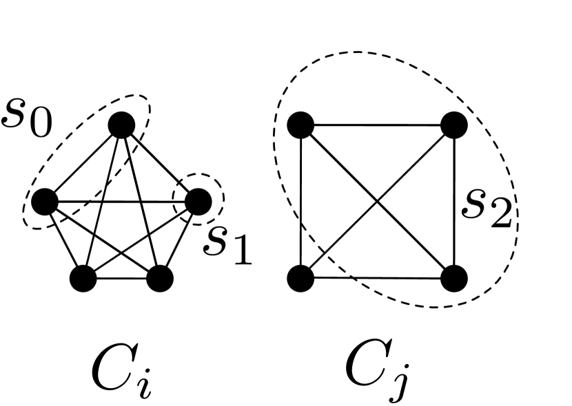
(a) Clique-shaped clusters.

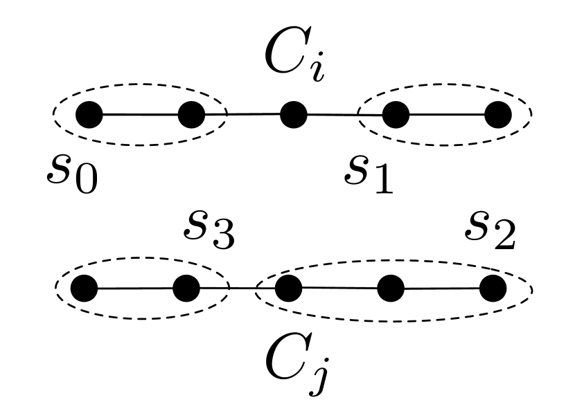
(b) Chain-shaped clusters.

Figure 1: Model-based separation. Figure 1(a) shows two clique-shaped clusters with data points as vertices in a graph. If $f$ separates the graph then $f(s_{0},s_{1})>\max[f(s_{0},s_{2}),f(s_{1},s_{2})]$ because $s_{0}$ and $s_{1}$ form a connected subgraph. In Figure 1(b), even if $f$ separates the graph, it is possible for $f(s_{0},s_{1})<f(s_{1},s_{2})$. However, $f(s_{1},s_{2})<f(s_{2},s_{3})$.

A visual illustration of both clique and chain style clusters is depicted in Figure 1. As we will see, chain structured connected components pose a challenge to existing incremental algorithms, something we resolve with Grinch (Section 3).

2.2 Cluster Trees

In most clustering problems, the appropriate number of clusters is unknown a priori. HAC addresses this uncertainty by building a cluster tree over data points.

Definition 2 (Cluster tree [24]).

A binary cluster tree $\mathcal{T}$ on a dataset $\mathcal{X}=\{x_{i}\}_{i=1}^{N}$ is a collection of subsets such that $C_{0}=\{x_{i}\}_{i=1}^{N}\in\mathcal{T}$ and for each $C_{i},C_{j}\in\mathcal{T}$ either $C_{i}\subset C_{j}$, $C_{j}\subset C_{i}$ or $C_{i}\cap C_{j}=\emptyset$. For any $C\in\mathcal{T}$, if $\exists C^{\prime}\in\mathcal{T}$ with $C^{\prime}\subset C$, then there exists two $C_{L},C_{R}\in\mathcal{T}$ that partition $C$.

Given a cluster tree, ${\mathcal{T}}$, any set of disjoint subtrees whose leaves cover $\mathcal{X}$ represents a valid clustering and is referred to as a tree consistent partition [18]. Thus, cluster trees compactly encode multiple alternative clusterings, allowing for a clustering to be selected as a post-processing step. Another advantage of using cluster trees is that they often facilitate efficient search and naturally group similar data points near one another in the hierarchy

We relate model-based separation, cluster trees and HAC in the following fact:

Fact 1.

Let $f$ be a linkage function that separates $G$. Then running HAC under $f$ returns a cluster tree, ${\mathcal{T}}$, such that the connected components of $G$ are a tree-consistent partition of ${\mathcal{T}}$.

To see why, notice that in each iteration of HAC, the highest scoring pair of remaining subtrees is merged. Since $f$ separates $G$, a merger resulting in a subtree that corresponds to a connected subgraph of $G$ has higher score than any merger resulting in a disconnected subgraph of $G$. Even though HAC can construct a cluster tree that contains the ground-truth clustering as a tree-consistent partition, the algorithm costs $O(n^{2}\log n)$ for general linkage functions and does not scale to large datasets. We will verify this claim empirically in our experiments (Section 4).

3 Rotations, Grafting and Grinch

In this section we derive an efficient, incremental algorithm called Grinch that can be used to construct clusterings under any linkage function. Like HAC, the backbone of Grinch is a cluster tree. We begin the discussion by analyzing a greedy, incremental variant of HAC and when it fails. Then, we introduce two subroutines, rotate and graft, that can be used to enhance robustness. Finally, we present our algorithm, Grinch.

3.1 Online HAC and Rotations

An efficient alternative to HAC is its online variant that merges each incoming data point with its nearest neighbor seen so far (Online). For now, let us consider the setting in which a nearest neighbor is found using a linkage function, $f$. Let $f$ separate a graph $G$ and let ground-truth clusters be cliques in $G$ (i.e., the data is strictly separated). Even in this simple case, Online may construct a cluster tree in which the ground-truth clustering is not a tree consistent partition. To see why, consider a stream in which the first two data points, $x_{1}$ and $x_{2}$, are of the same ground-truth cluster and the third data point, $x_{3}$ is of a different cluster. Assume, without loss of generality, that Online adds $x_{3}$ as a sibling of $x_{1}$. Then the ground-truth clustering is not a tree consistent partition of the resulting tree (and all subsequent trees).

To recover from such mistakes, local tree rearrangements may be applied. Previous work uses rotations, which swap a child and its aunt in the tree, to correct local errors induced by unfavorable arrival order [22]. While originally designed to be used with pairwise distances, the condition under which rotations should be applied can be extended to linkage functions:

$$f(v,\texttt{s}(v))<f(v,\texttt{aunt}(v))$$ (1)

where the functions $\texttt{s}(\cdot)$ and $\texttt{aunt}(\cdot)$ return the sibling and aunt of their input, respectively. In words, if a node $v\in{\mathcal{T}}$ achieves a higher score under $f$ with its aunt than with its sibling, then the aunt and sibling should be swapped. Now, let us revisit the example above. Since $x_{1}$ and $x_{2}$ are both vertices in the same clique in $G$, they are connected by an edge. Then, by model-based separation, $f(x_{1},x_{2})>f(x_{1},x_{3})$, so a rotation will be applied, producing a tree that contains the ground-truth clustering.

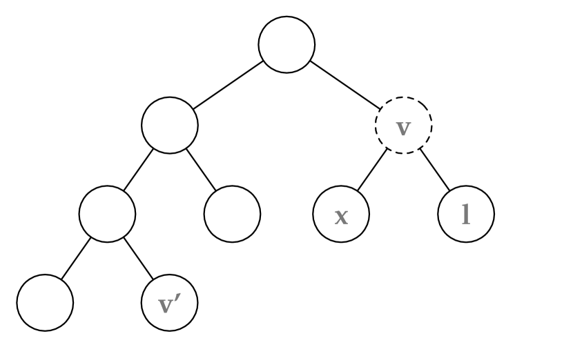
(a) $x$ added to cluster tree.

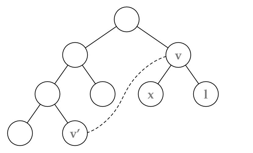
(b) $v$ finds nearest node $v^{\prime}$.

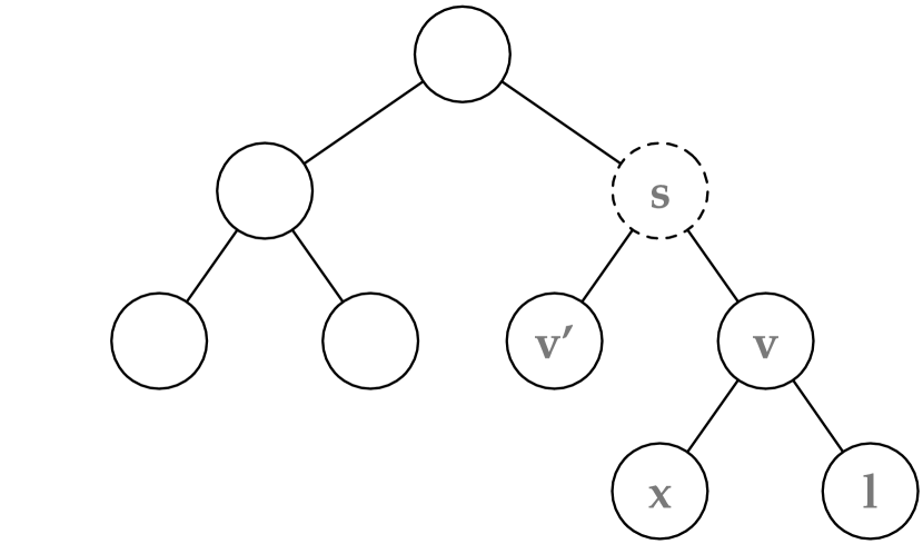
(c) $v$ is grafted to $v^{\prime}$.

Figure 2: The graft subroutine. Dotted lines denote new nodes and mergers. Before $x$ is added to tree, $l$ and $v^{\prime}$ reside in disjoint subtrees even though they belong to the same ground-truth cluster. The addition of $x$ creates the subtree with root $v$ and initiates the graft subroutine.

Unfortunately, the Online algorithm, augmented with the ability to performs rotations (Rotate), cannot always recover the connected components of a graph that is separated by $f$. In particular, Rotate cannot reliably recover chains (Example 2). By virtue of being a local operation, rotations can only be used to provably recover connected components that are clique-structure.

3.2 Subtree Grafting

We introduce a non-local tree rearrangment called a graft, which facilitates the discovery of chain-structured connected components. At a high level, the graft procedure with respect to a node $v\in{\mathcal{T}}$ searches ${\mathcal{T}}$ for a node $v^{\prime}$ that is both similar to $v$ and dissimilar from its current sibling, $\texttt{s}(v^{\prime})$. If such a subtree is found, $v^{\prime}$ is disconnected from its parent and made a sibling of $v$. A visual illustration of a successful graft is depicted in Figure 2.

In detail, a graft searches the leaves of ${\mathcal{T}}$ for the nearest neighbor leaf of $v$ called $l$. Then it checks whether the following holds:

$$f(v,l)>\max[f(v,\texttt{s}(v)),f(l,\texttt{s}(l))]$$ (2)

i.e., $v$ and $l$ prefer each other to their current siblings according to $f$. If the condition succeeds, merge $v$ and $l$. If the condition fails because $l$ prefers its sibling to $v$, retest the condition at $v$ and $l$’s parent, $\texttt{par}(l)$; if the condition fails because $v$ prefers its sibling to $l$, then retest the condition at $\texttt{par}(v)$ and $l$. Continue to check recursively until the condition succeeds or until the first time two nodes, $v_{1}$ and $v_{2}$, are reached such that one is the ancestor of the other. Pseudocode for the graft subroutine can be found in Algorithm 1. In the algorithm, par returns the parent of a node in the tree, lca returns the lowest common ancestors of its arguments and makeSib merges its arguments and returns their new parent. NN performs a nearest neighbor search and constrNN performs a nearest neighbor search that excludes its second argument from the result.

3.3 Tree Restructuring

While the graft subroutine facilitates discovery of chain-structured clusters, poorly structured trees are susceptible to having the graft subroutine disconnect previously discovered ground-truth clusters. As an example, consider Figure 3, in which $\texttt{lvs}(v)$ form the connected subgraph $C_{i}$ (i.e., they all belong to the same ground-truth cluster). Consider $v$’s left child, $v.l$, and its descendants, which form a disconnected subgraph. An attempt to graft either descendent, $x_{1}$ or $x_{2}$, may succeed, even when initiated from a node (not depicted) whose descendants are not connected to $C_{i}$. After such a graft, ${\mathcal{T}}$ cannot contain a tree-consistent partition that matches the ground-truth clustering.

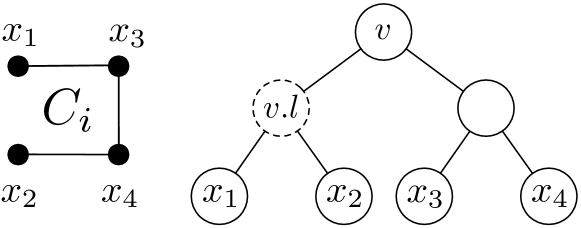
Figure 3: Poorly structured tree. Even though $v$’s leaves form a connected subgraph of the graph on the left of the Figure (i.e., they all belong to cluster $C_{i}$), $v.l$’s descendent leaves, $x_{1}$ and $x_{2}$, are disconnected. An attempt to graft either $x_{1}$ or $x_{2}$ from a node whose descendants are not members of $C_{i}$ may succeed.

Algorithm 1 graft $(v,{\mathcal{T}},f)$

  $l=\texttt{constrNN}(v,\texttt{lvs}(v),f,{\mathcal{T}})$

  $v^{\prime}=\texttt{lca}(v,l)\texttt{; st = v}$

  while $v\neq v^{\prime}\wedge l\neq v^{\prime}\wedge\texttt{s}(v)\neq l$ do

     if $f(v,l)>\max[f(v,\texttt{s}(v),f(l,\texttt{s}(l))]$ then

        $z=\texttt{s}(v)\texttt{; }v\,=\texttt{merge}(v,l)$

        $\texttt{restruct}(z,\texttt{lca}(z,v),f)$

        break

     if $f(v,l)\,<\,f(l,\texttt{s}(l))$ then

        $l\,=\texttt{par}(l)$

     if $f(v,l)\,<\,f(v,\texttt{s}(v))$ then

        $v\,=\texttt{par}(v)$

  if $v==st$ then

     Output: $v^{\prime}$

  else

     Output: $v$

Notice that a subtree can defend against spurious grafts by ensuring that each of its descendant subtrees is connected. For example, in Figure 3, if $x_{2}$ and $x_{3}$ were swapped, then each descendant subtree of $v$ would be connected. Moreover, after such a swap, grafts from nodes whose descendants were not part of $C_{i}$ would necessarily fail (assuming that $f$ separates the graph).

During tree construction, the only step that can result in a connected subtree with disconnected descendants is the graft subroutine (a rigorous proof is included in the supplement). We introduce the restruct (restructure) subroutine, which is performed after a successful graft, and reorganizes a subtree with the intent of making each of its descendants connected. Let $v^{\prime}$ be a node that was just grafted, $v$ be the previous sibling of $v^{\prime}$ (i.e., before the graft) and let $r=\texttt{lca}(v,v^{\prime})$ be the current least common ancestor of $v$ and $v^{\prime}$. restruct is initiated from $v$. First, the siblings of the ancestors of $v$ (until $r$) are collected. Then, we find the node in the collection most similar to $v$. If that node is more similar to $v$ than $v$’s current sibling (according to $f$), the two are swapped. The intuition here is that if a graft left $v$ and its new sibling disconnected, then the swap serves as a mechanism to restore the connectedness of $v$’s parent. Such swaps are attempted from the ancestors of $v$ until $r$. Pseudocode appears in Algorithm 2.

3.4 Grinch

Using the rotate, graft and restruct tree rearrangement routines discussed in Section 3, we derive a new algorithm called Grinch, which stands for: Grafting and Rotation-based INCremental Hiearchical clustering. The steps of the algorithm are as follows: when a new record, $x_{i}$, arrives, find $x_{i}$’s nearest neighbor, $l$, among the leaves of ${\mathcal{T}}$. Add $x_{i}$ to ${\mathcal{T}}$ as a sibling of $l$. Then, apply the rotate subroutine while Equation 1 is true. Finally, attempt to graft recursively from each ancestor of $x_{i}$. Each time a graft is successful, restructure the tree to group similar items together. Pseudocode for Grinch can be found in Algorithm 3.

Algorithm 2 restruct$(z,r,f)$

  while $z!=r$ do

     $as=\{\texttt{s}(a)\,\texttt{for}\,a\in\texttt{ancs}(z)\backslash\texttt{ancs}(r)\}$

     $m=\mathop{\mathrm{argmax}}_{a\in as}f(z,a)$

     if $f(z,\texttt{s}(z))\,<\,f(z,m)$ then

        $\texttt{swap}(\texttt{s}(z),m)$

     $z=\texttt{par}(z)$

Algorithm 3 Insert$(x_{i},{\mathcal{T}},f)$

  $l=$ NN$(x_{i},f,{\mathcal{T}})\texttt{; }t=\texttt{ makeSib}(x_{i},l)$

  while $f(x_{i},\texttt{s}(x_{i}))<f(\texttt{aunt}(x_{i}),\texttt{s}(x_{i}))$ do

     rotate $(x_{i},\texttt{aunt}(x_{i}))$

  $p=\texttt{par}(x_{i})$

  while $p\neq\texttt{null}$ do

     $\texttt{curr}=\texttt{graft}(p,{\mathcal{T}},f)$

Theorem 1.

Let $\mathcal{X}=\{x_{i}\}_{i=1}^{N}$ be a dataset with ground-truth clustering $\mathcal{C}^{\star}=\{C_{1},\cdots,C_{k}\}$. Let $f$ separate a graph $G$ on vertices $\mathcal{X}$ and let each cluster $C\in\mathcal{C}^{\star}$ be a connected component in $G$. Then Grinch recovers a cluster tree such that $\mathcal{C}^{\star}$ is a tree consistent partition of ${\mathcal{T}}$ regardless of the input order.

The proof of Theorem 1 can be found in the appendix.

4 Experiments

We experiment with Grinch to assess its scalability and accuracy. We begin by demonstrating that Grinch outperforms other incremental clustering algorithms on a synthetic dataset. Observing that some of the steps of Grinch are underutilized, we present 4 approximations of Grinch’s algorithmic components. We apply each approximation in turn and show that together they dramatically improve Grinch’s scalability without compromising its clustering quality. Then, we compare the approximate variant of Grinch to state-of-the-art large scale hierarchical clustering methods. To showcase the flexibility of Grinch, we also provide experimental results in entity resolution, where the linkage function is learned. Finally, we provide analysis of the graft subroutine–Grinch’s distinguishing feature–and perform experiments to demonstrate the algorithm’s robustness.

Dendrogram Purity

Before beginning, we briefly review dendrogram purity, a preferred method of holistically evaluating hierarchical clusterings [6, 18, 22]. Dendrogram purity is computed as follows: Let $\mathcal{C}^{\star}=\{C_{1},\cdots,C_{k}\}$ be the ground-truth clustering of a dataset $\mathcal{X}$, and let $\mathcal{P}^{\star}=\{(x,x^{\prime})|x,x^{\prime}\in\mathcal{X},\ \mathcal{C}^{\star}(x)=\mathcal{C}^{\star}(x^{\prime})\}$ be the set of all data point pairs that belong to the same ground-truth clusters. Then the dendrogram purity (DP) of a cluster tree, ${\mathcal{T}}$ is:

$$\textrm{DP}({\mathcal{T}})=\frac{1}{|\mathcal{P}^{\star}|}\sum_{(x,x^{\prime})\in\mathcal{P}^{\star}}\texttt{pur}(\texttt{lvs}(\texttt{lca}(x,x^{\prime})),\mathcal{C}^{\star}(x))$$

where $\texttt{lca}(x,x^{\prime})$ returns the least common ancestor of $x$ and $x^{\prime}$ in ${\mathcal{T}}$, $\texttt{lvs}(\cdot)$ returns the descendant leaves of its argument, and $\texttt{pur}(\cdot,\mathcal{C}^{\star}(x))$ takes a collection of leaves and computes the fraction that belong to ground-truth cluster $\mathcal{C}^{\star}(x)$.

4.1 Synthetic Data Experiment

In our first experiment, we compare Grinch to other incremental hierarchical clustering algorithms on a synthetic dataset in order to begin to understand Grinch’s empirical performance characteristics in a controlled manner. The data is generated so that it satisfies model-based separation with respect to cosine similarity. In particular, the dataset contains 2500 10000-dimensional binary vectors that belong to 100 clusters, with 25 points per cluster. Points in cluster $k$ have bits $100k$ to $100(k-1)$ set randomly to 1 with probability $0.1$. All other bits are set to 0. This way, across cluster points have cosine similarity 0 and within cluster points can have either 0 or non-zero cosine similarity. In other words, two points, $x_{1}$ and $x_{2}$, in the same cluster can appear to be dissimilar and end up in distant regions of the tree. The representation of each internal node in the Grinch tree is the sum of the vectors of its descendent leaves. Thus, compute the cosine similarity between two nodes $v$ and $v^{\prime}$ as the cosine similarity between their aggregated vectors ( we refer to this as cosine linkage in the following sections ). We compare Grinch, Rotate and Online.

The experimental results reveal that Grinch achieves perfect dendrogram purity (1.0), which is expected given Grinch’s correctness guarantee. Rotate achieves a dendrogram purity of 0.872 while Online achieves 0.854. Rotate and Online do not construct trees of perfect purity because of their inability to globally rearrange a cluster hierarchy.

4.2 Approximations

Some of the algorithmic steps of Grinch, which are required to prove its correctness, are seldom invoked in practice. For example, and perhaps expectedly, a graft is unlikely to succeed between two nodes close to the root of the tree. Therefore, we introduce handful of approximations designed to have little effect on the quality of the clusterings constructed by Grinch, but also designed to make the algorithm significantly faster in practice.

1. Capping. Recursive subroutines like graft and rotate improve performance, but they are also computationally expensive to check, and often fail. Moreover, we notice that tree rearrangements that occur close to the root do not have a significant, instantaneous effect on dendrogram purity. Therefore, we introduce rotation, graft and restructure caps, which prohibit rotations, grafts and restructures from occurring above a height, $h$.

2. Single Elimination Mode. The graft subroutine generally improves Grinch’s clustering performance, and is essential in attaining perfect purity on the synthetic dataset, but we find that graft attempts are rejected many more times than they are accepted. However, at times, we observe that a sequence of recursive grafts are accepted when initiated close to the leaves. Therefore, to limit the number of attempted grafts while retaining these graft sequences, we introduce single elimination mode. In this mode, the recursive grafting procedure terminates after a graft between $v$ and $v^{\prime}$ fails because both prefer their current siblings to a merge.

3. Single Nearest Neighbor Searching. Grinch makes heavy use of nearest neighbor search under the linkage function $f$. Rather than perform nearest neighbor search anew for each graft, when a data point arrives, we perform a single $k$-NN search ($k\in[25,50]$) and only consider these nodes during subsequent grafts (until the next data point arrives).

4. Navigable Small World Graphs. Instead of performing nearest neighbor computations exactly, we can perform them approximately. To this end, we employ a navigable small world nearest neighbor graph (NSW)–a data structure inspired by decentralized search in small world networks [31, 20, 21]. To find the nearest neighbor of a data point, $x_{i}$, in an NSW, begin at a random node, $v$. If the similarity between $x_{i}$ and $v$ is maximal among all neighbors of $v$, terminate; otherwise, move to the neighbor of $v$ most similar to $x_{i}$. To insert a new data point, $x_{j}$, find its $k$ nearest neighbors and add edges between those neighbors and a new data point [27]. Thus, NSWs are constructed online. In practice, we simultaneous construct a hierarchical clustering and an NSW over the data points stored in the tree’s leaves.

ALOI
Approx.	DP	Time (s)	# Rotate	# Graft	# Restr.
Grinch (No Approx).	0.533	85.371	7107	2435	1088
w/ Cap (100)	0.533	48.452	6495	2157	686
w/ Single Elimn	0.534	39.019	6574	1586	533
w/ Single NN	0.540	22.226	6441	1516	570
w/ no Restruct	0.538	14.292	6477	1634	0
w/ no Graft	0.506	12.748	6747	0	0
w/ no Rotate	0.442	14.793	0	0	0
Synthetic
Approx.	DP	Time (s)	# Rotate	# Graft	# Restr.
Grinch (No Approx).	1.0	160.307	2558	578	203
w/ Cap (100)	0.993	164.328	2558	578	194
w/ Single Elimn	0.997	157.622	2523	526	184
w/ Single NN	0.993	83.014	2517	415	148
w/ no Restruct	0.993	82.262	2476	426	0
w/ no Graft	0.872	82.055	2259	0	0
w/ no Rotate	0.854	80.526	0	0	0

Table 1: Ablation. Each row in the table represents Grinch with the corresponding approximation applied in addition to all approximations contained in previous rows. The first 4 approximations significantly decreases the computational cost of Grinch, but do not compromise DP. The ablation is performed for the first 5000 points of ALOI and the Synthetic datasets.

To measure the effects of our approximations on the speed and quality of the resulting algorithm, we conduct the following ablation. We run Grinch on our synthetically generated dataset as well as a random 5k subset of the ALOI [13] dataset and measure dendrogram purity, time, and the number of calls made to rotate, graft and restruct. We repeat the procedure multiple times, each time adding one of the following approximations, in order: capping, single elimination, single nearest neighbor search and approximate nearest neighbor search. Capping and is performed at height 100. We also experiment with removal of the graft and rotate subroutines.

The result of the ablation is contained in Table 1. We observe that, for both datasets, each of the approximations reduces the computational cost of algorithm without effecting the resulting DP. However, once grafts are removed, the DP drops by 3% on ALOI and 12% on the synthetic datasets. When rotate is also removed, DP drops by an additional 6% and 2%, respectively.

Having verified that on a subset of ALOI our approximations improve scalability at little expense in terms of dendrogram purity, in the following experiments we report results for Grinch in single elimination mode and with the rotation cap set to $h=100$.

4.3 Large Scale Clustering

Alg. (link.)	CovType	ILSVRC12 (50k)	ALOI	Speaker	ImgNet (100k)
Grinch (Avg)	0.43 $\pm$ 0.00	0.557 $\pm$ 0.003	0.504 $\pm$ 0.002	0.480 $\pm$ 0.003	0.065 $\pm$ 0.00
Grinch (CS)	0.43 $\pm$ 0.00	0.544 $\pm$ 0.005	0.499 $\pm$ 0.003	0.478 $\pm$ 0.003	0.062 $\pm$ 0.00
Rotate (Avg)	0.43 $\pm$ 0.01	0.545 $\pm$ 0.004	0.476 $\pm$ 0.004	0.407 $\pm$ 0.003	0.063 $\pm$ 0.00
Rotate (CS)	0.44 $\pm$ 0.01	0.513 $\pm$ 0.007	0.472 $\pm$ 0.003	0.406 $\pm$ 0.003	0.062 $\pm$ 0.00
Online	0.44 $\pm$ 0.01	0.527 $\pm$ 0.00	0.435 $\pm$ 0.004	0.317 $\pm$ 0.002	0.0589
Perch [22]	0.45 $\pm$ 0.00	0.53 $\pm$ 0.003	0.44 $\pm$ 0.004	0.37 $\pm$ 0.002	0.065$\pm$0.00
Perch-BC [22]	0.45 $\pm$ 0.00	0.36 $\pm$ 0.005	0.37 $\pm$ 0.008	0.09 $\pm$ 0.001	0.03 $\pm$ 0.00
MB-HAC (Best) [22]	0.44 $\pm$ 0.01	0.43 $\pm$ 0.005	0.30 $\pm$ 0.002	0.01 $\pm$ 0.002	—
HAC (Avg) [22]	–	0.54	–	0.55	–

Table 2: Dendrogram Purity results for Grinch and baseline methods. We compare two linkage functions: approximate average linkage (Avg) and cosine similarity linkage (CS).

We compare Grinch with the following 4 algorithms: Online - an online hierarchical clustering algorithm that consumes one data point at a time and places it as a sibling of its nearest neighbor; Rotate - an incremental algorithm that places a data point next to its nearest neighbor and then performs rotations until Equation 1 holds; MB-HAC - the mini-batch version of HAC, which keeps a buffer of size $b$, runs a single step of HAC using the data points in the buffer and then adds the next record to the buffer; HAC - best-first, bottom-up hierarchical agglomerative clustering and Perch - a state-of-the-art large scale hierarchical clustering method.

We run each algorithm on 5 large scale clustering datasets: CovType, a datset of forest covertype, ALOI [13], a 50K subset of the Imagenet ILSVRC12 dataset [28] and the Speaker dataset [14], and a 100K subset of ImageNet containing all 17K classes not just the subset in ILSVRC12. Datasets have 500K, 50K, 100K, 36K, and 100K instances, respectively. We run each HAC variant under two different linkage functions: average linkage and cosine linkage. To compute the cosine similarity between two nodes, $v$ and $v^{\prime}$, first, for each node, compute the sum of the vectors contained at their descendant leaves. Then, compute the cosine similarity between the aggregated vectors.

Results are displayed in Table 2, where we record the dendrogram purity averaged over 5 replicates of each algorithm, where for each replicate we randomize the arrival order of the data. The table reveals that Grinch–under both linkage functions–outperforms the corresponding versions of Rotate and Online on all datasets except for on the CovType dataset where the methods all seem to perform equally well. This underscores the power of the graft subroutine. Grinch with approximate nearest neighbor search even outperforms Perch, which uses exact nearest neighbor search, on ALOI. Recall that, unlike the HAC variants, Perch employs a specific linkage function. Seeing as the HAC variants outperform Perch on Speaker suggests that the ability to equip various linkage functions can be advantageous. HAC is best on Speaker, but cannot scale to ALOI.

4.4 Author Coreference

Bibliographic databases, like PubMed, DBLP, and Google Scholar, contain citation records that must be attributed to the corresponding authors. For some records, the attribution process is easy, but for many others, the identities of a publication’s authors are ambiguous. For example, DBLP contains hundreds of citations written by different authors named “Wei Wang” that currently cannot be disambiguated [2]. Intuitively, author coreference datasets often exhibit chain like structures because a single citation written by a prolific author (perhaps in a short-lived collaboration) may only be similar to a small number of that author’s other citations and dissimilar from the rest.

Following previous work, we train a linkage function to predict the likelihood that a group of citation records were all written by the same author [9, 29, 32]. We train our model by running HAC and, at each step, use the model to predict the precision of merging two groups of records. (A similar training technique was previously proposed for entity and event coreference [25].) Our model has access to features like: coauthor names and publication title, venue, year, etc.

We compare the 5 HAC variants in author coreference on two datasets with labeled author identities: Rexa [9] and PSU-DBLP [16]. As is standard in author coreference we evaluate the methods using the pairwise F1-score of a predicted flat clustering against the ground-truth clustering, which is the harmonic mean of precision and recall. To compute pairwise F1-score, each pair of citations that appear in both the same ground-truth and predicted clusters is considered a true positive; each pair of citations that belong to different ground-truth clusters but the same predicted cluster is considered a false positive. None of the authors represented in the test set, have any publications in the training set.

Figure 3 shows the precision, recall, and pairwise F1-score achieved by each method. The results show that Grinch outperforms the other scalable methods on both datasets and even outperforms HAC on DBLP. This behavior may stem from overfitting of the learned linkage function, which is exploited by HAC; since Grinch only approximates HAC, it can be thought of as a form of regularization. Again, we observe that Grinch outperforms Online and Rotate on both datasets underscoring the importance of the rotate and graft procedures.

	Rexa			DBLP
Algorithm	Pre	Rec	F	Pre	Rec	F
Grinch	0.808	0.883	0.844 $\pm$ 0.004	0.809	0.620	0.701 $\pm$ 0.013
Rotate	0.864	0.641	0.734 $\pm$ 0.057	0.876	0.554	0.678 $\pm$ 0.019
Online	0.850	0.209	0.331 $\pm$ 0.094	0.827	0.151	0.255 $\pm$ 0.027
MB-HAC-Med.	0.807	0.881	0.843 $\pm$ 0.0009	0.375	0.631	0.461 $\pm$ 0.072
MB-HAC-Sm.	0.922	0.333	0.483 $\pm$ 0.061	0.697	0.151	0.247 $\pm$ 0.004
HAC	0.805	0.887	0.844	0.741	0.600	0.664

Table 3: Precision, recall and F-Score of various methods on the Rexa and DBLP datasets.

4.5 Significance of Grafting

The results above indicate that Grinch–even when employing a number of approximations–constructs trees with higher dendrogram purity than other scalable methods in a comparable amount of time. Interestingly, Grinch only differs from rotate in its use of the graft (and subsequent restruct) subroutine. To better understand the significance of grafting, we compare Grinch and rotate on the first 5000 points of ALOI.

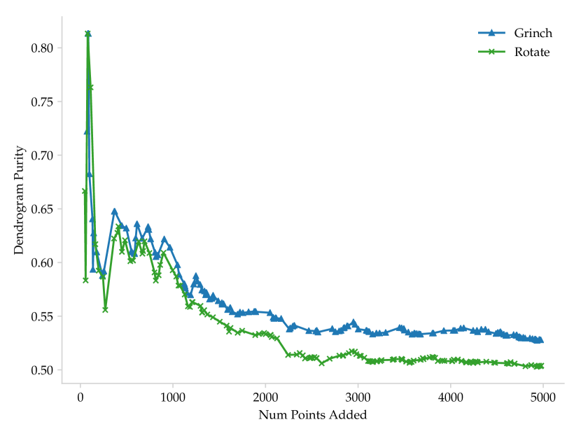
(a) Dendrogram purity per point.

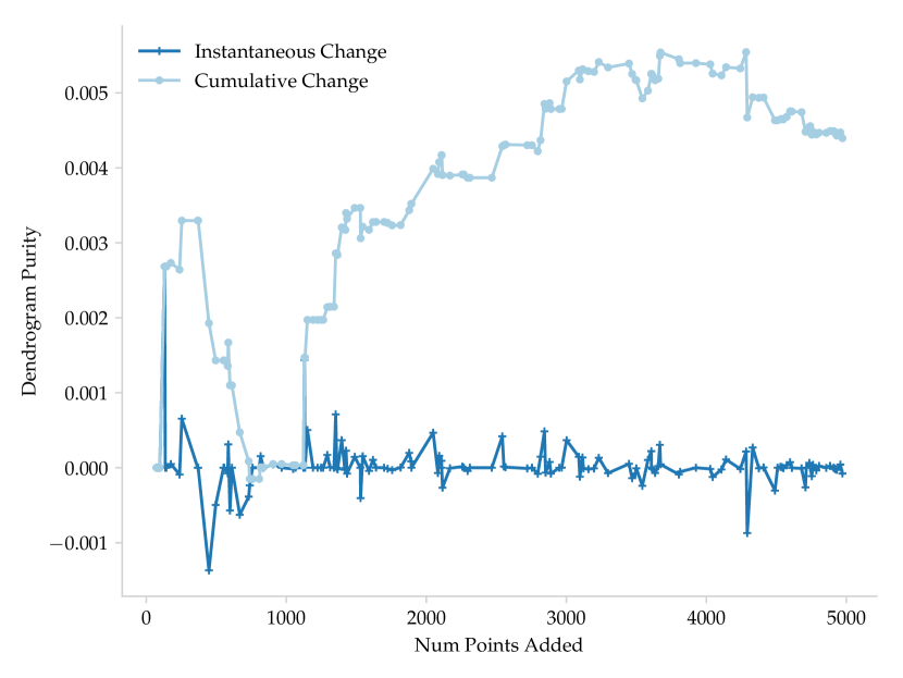
(b) Instant./cumulative change in DP due to grafts.

Figure 4: Figure 4(a) shows the dendrogram purity of two trees, one built by Grinch and the other built by rotate, on the first 5000 points of ALOI. The dendrogram purity of the tree built Grinch is greater than that of the tree built by rotate. Figure 4(b) plots the instantaneous and cumulative change in dendrogram purity due to grafts. While Grinch achieves  3% larger dendrogram purity than rotate

Figure 4(a) shows that dendrogram purity as a function of the number of data points inserted for both Grinch and rotate and the first 5000 points of ALOI. Echoing the results above, by  1000 points, Grinch dominates rotate.

Figure 4(b) shows the instantaneous and cumulative change in dendrogram purity due to grafts made by Grinch. That is, for the $i$th data point, $x_{i}$, we record the dendrogram purity after $x_{i}$ is inserted and rotations are performed (i.e., what would be executed by rotate). Then, we perform grafting (if appropriate) and record the dendrogram purity after all recursive grafts have been completed. The difference between the dendrogram purity after grafting and before grafting (but after rotations) is the instantaneous change in dendrogram purity due to grafts; the sum of instantaneous changes is the cumulative change.

Note the $y$-axis of Figure 4(b), which reveals that even the most instantaneously significant grafts only lead to minute changes in dendrogram purity (of about 0.001). Moreover, after 5000 points, the cumulative change in dendrogram purity due to grafts is less than 0.005–hardly accounting for the difference in dendrogram purity between the tree built by Grinch and the tree built by rotate (of  0.03). We conclude from these measurements that the increase in performance due to the graft subroutine is related to the rearrangement of small numbers of points. These rearrangements do not immediately have significant impact on dendrogram purity, but they do have significant long-term affects. To make this hypothesis more concrete, consider the case in which two dissimilar data points from the same cluster are split between two distant regions of the tree early on in clustering. The points are never merged (via a graft) and so each point draws a significant portion of the cluster’s other data points to its location in the tree. This has dire consequences with respect to dendrogram purity. If a graft is performed early on to correct the split, an adverse scenario like this can be averted.

4.6 Robustness

For completeness, we perform an experiment used in previous work to test an incremental clustering algorithm’s robustness to data point arrival order [22]. In the experiment, a dataset is ordered in two specific ways:

Round-Robin

Randomly determine an ordering of ground-truth clusters. Then, construct a data point arrival order such that the $i$th data point is a member of cluster $i$ mod $K$, where $K$ is the number of clusters and mod returns the remainder when its first argument is divided by its second.

Sorted

Randomly determine an ordering of ground-truth clusters. All points of cluster $C_{i}$ arrive before any point of cluster $C_{i+1}$ arrives.

Method	Round.	Sort.
Grinch	0.503	0.457
Perch	0.446	0.351
MB-HAC (5K)	0.299	0.464
MB-HAC (2K)	0.171	0.451

Table 4: DP for adversarial arrival orders (ALOI).

As in previous work, we perform a robustness experiments with the ALOI dataset. Table 4 shows that Grinch achieves higher dendrogram purity than both Perch and mini-batch HAC (with 2 different batch sizes) on data ordered using the Round Robin ordering scheme. Under this arrival order, MB-HAC performs poorly showing its lack of robustness. When the data is in Sorted order–which makes for easier clustering for MB-HAC–Grinch outperforms Perch and is competitive with MB-HAC.

5 Related Work

The family of online and incremental clustering methods is diverse, however all algorithms in this family optimize for specific linkage functions. Perch, from which the rotate procedure is inspired, performs rearrangments to satisfy a condition similar to complete-linkage [22]. BIRCH is another top-down hierarchical clustering algorithm that attempts to minimize a $k$-center style cost at each node in the tree [35]. BIRCH also includes a non-greedy reassignment step but has been shown to produce low quality trees in practice. Liberty et al propose a flat clustering algorithm that optimizes $k$-means cost. Since their algorithm runs in the online setting, after a data point arrives and is assigned to a cluster, it may never be reassigned [26]. While not incremental, some work focuses on designing highly scalable algorithms for specific linkage functions. Particular attention is paid to single-linkage because of its connection to the minimum spanning tree problem. For example, recent work develops massively parallel algorithms for single-linkage [4].

When clustering with linkage functions, probabilistic approaches can provide an alternative to HAC. For example, split-merge Markov Chain Monte Carlo (MCMC) methods perform clustering by randomly splitting and merging clusters according to a proposal function [19]. An algorithm similar to split-merge MCMC has even been used for author coreference [32]. This algorithm employs a custom linkage function on structured records and works by maintaining a forest–each tree corresponding to a cluster–and randomly proposing mergers and splits of various branches. Unlike Grinch, this algorithm relies on sampling to escape local minima. As the number of items grows, the likelihood of sampling a merge or split that will be accepted decreases rapidly.

Our work is partially inspired by complex linkage functions that are used for clustering. One example is Bayesian hierarchical clustering (BHC)–a recursive, probabilistic, hierarchical model for data [18]. Fitting BHC models is performed by running HAC with BHC as the linkage function. Because HAC is inefficient, randomized approaches for fitting BHC have also been proposed, but each of these methods still runs HAC as a subroutine on small, randomly selected subsets of data [17]. HAC-style algorithms are also used to do probabilistic, hierarchical community detection and alongside learned models for entity resolution [5, 25].

Model-based separation is related to recently proposed definitions of perfect hierarchical clustering structure [8, 30], in which pairwise similarities between data points lead to a tree that can be discovered by HAC that has minimal cost. The costs used in these works are variants of Dasgupta’s cost [10]. Perfect hierarchical clustering structures are a special case of model-based separation, in which single-, average-, or complete-linkage is used. Model-based separation is strictly more general, allowing for linkage functions that compute the similarity of two point sets arbitrarily, rather than as a function of pairwise data point similarities.

6 Conclusion

This paper introduces Grinch, an incremental algorithm for hierarchical clustering under any linkage function. The algorithm relies on two subroutines, rotate and graft, that help it to discover complex cluster structure regardless of data arrival order. We introduce model-based separation for clustering with linkage functions and prove that Grinch always returns a tree with perfect dendrogram purity when running in the separated setting. We describe an efficient implementation of Grinch and present an empirical evaluation demonstrating that Grinch is more accurate than other baseline approaches and more scalable than HAC. We believe that Grinch is an asset for large clustering problems in which the data points engage in complicated relationships and clusters are best modeled by learned linkage function.

Source code for Grinch is available at: https://github.com/iesl/grinch.

Appendix A Proof of Theorem 1

Define the following properties:

Definition 3 (Strong Connectivity).

Let $G=(\mathcal{X},E)$ be a graph and let ${\mathcal{T}}[v]$ be a tree rooted at a node $v$ with leaves, $\texttt{lvs}(v)=\mathcal{X}^{\prime}\subseteq\mathcal{X}$. $v$ is connected if $\mathcal{X}^{\prime}$ is a connected subgraph of $G$. $v$ is strongly connected if every descendant of $v$ is connected. $v$ is a maximal strongly connected node if $v$ is strongly connected and $\texttt{par}(v)$ is not strongly connected. Finally, the tree ${\mathcal{T}}$ satisfies strong connectivity if all connected nodes in ${\mathcal{T}}$ are strongly connected.

Definition 4 (Completeness).

Let $G=(\mathcal{X},E)$ be a graph and let ${\mathcal{T}}[v]$ be a tree rooted at a node $v$ with leaves, $\texttt{lvs}(v)=\mathcal{X}^{\prime}\subseteq\mathcal{X}$. Then $v$ is complete if $\mathcal{X}^{\prime}$ is a connected component in $G$. The tree ${\mathcal{T}}$ satisfies completeness if the set of connected components of $G$ are (the leaves of) a tree consistent partition of ${\mathcal{T}}$.

According to Theorem 1, Grinch always constructs a tree that satisfies completeness. To prove the theorem, we will show that after the addition of each new data point, the resulting tree satisfies strong connectivity and completeness. We analyze various subroutines of Grinch and demonstrate how they preserve strong connectivity, completeness or both. In the proceeding lemmas and proofs, let $G=(\mathcal{X},E)$ be a graph and let $f$ be a model that separates $G$.

Lemma 1 (Rotation Lemma).

Let ${\mathcal{T}}$ be a tree with $\texttt{lvs}({\mathcal{T}})=\mathcal{X}$, and let $x$ be a new data point to be added to ${\mathcal{T}}$. Then all nodes that were strongly connected before the addition of $x$ are strongly connected after the addition of $x$, i.e., rotations preserve strong connectivity.

Note: while rotations preserve strong connectivity, they do not guarantee completeness. Therefore rotations are insufficient for proving Theorem 1.

Proof.

Let $v$ be a maximal strongly connected node in ${\mathcal{T}}$ and assume that $x$ is added as a leaf of $v$ (rotations have not yet been applied). Consider two cases: (1) there exists an edge between $x$ and some leaf in $\texttt{lvs}(v)$, and (2) there does not exist an edge between $x$ and any leaf in $\texttt{lvs}(v)$.

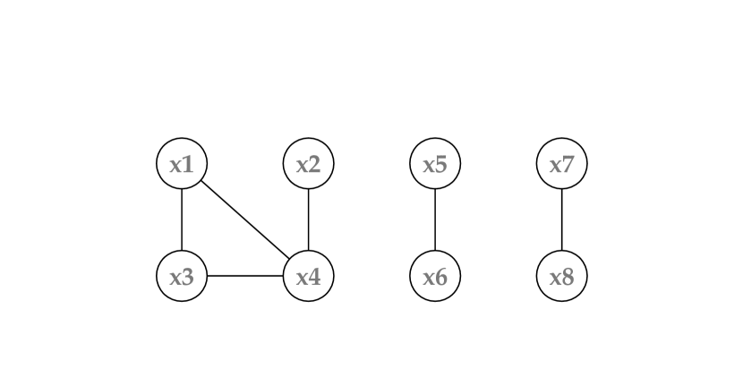
(a) A graph $G=(\mathcal{X},E)$.

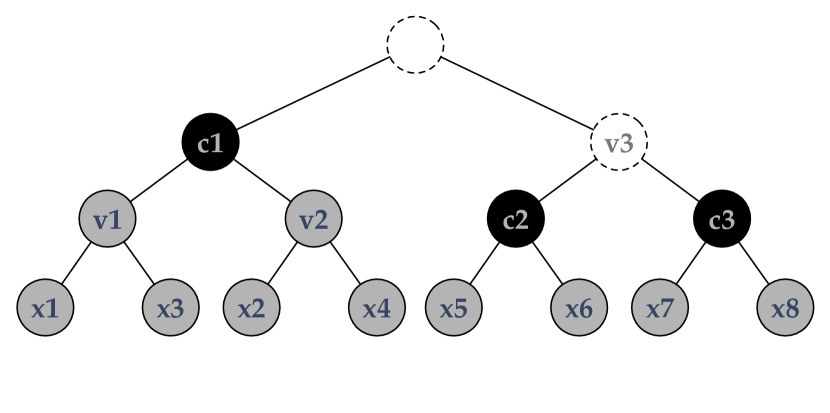
(b) Strongly connected & complete.

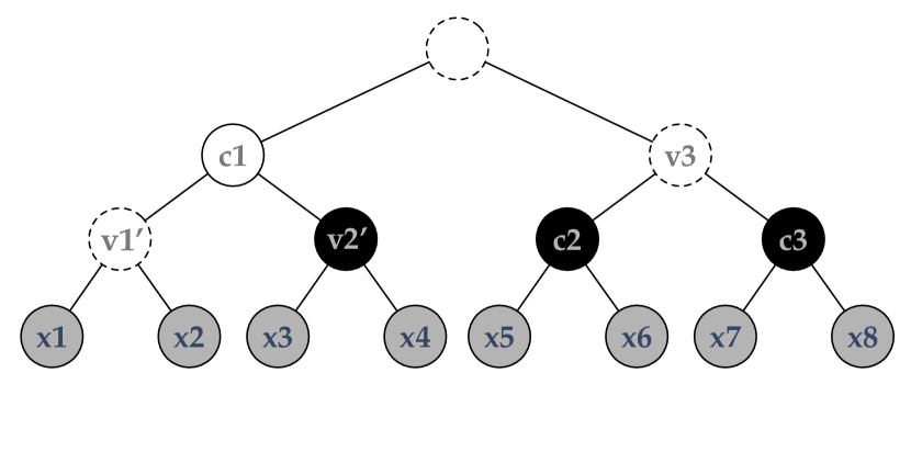
(c) Complete only.

Figure 5: A graph $G$ with 3 connected components (Figure 5(a)). In Figure 5(b) and Figure 5(c), black-filled nodes are maximal, gray-filled nodes are strongly connected, nodes with no fill and solid borders are connected (but not strongly), and nodes with dashed borders are disconnected. The tree in Figure 5(b) satisfies strong connectivity and completeness. The tree in Figure 5(c) does not satisfy strong connectivity because $v_{1}$ is disconnected.

Case 1:

Let $L\subseteq\texttt{lvs}(v)$ be the set of $v$’s descendant leaves to which $x$ is connected. Then $x$ is initially added as a sibling of its nearest neighbor leaf, $x^{\prime}$, and $x^{\prime}\in L$ because $f$ separates $G$. $\texttt{par}(x)$ is strongly connected because there exists an edge between $x$ and $x^{\prime}$.

The addition of $x$ does not disconnect $v$ or any strongly connected descendant of $v$. To see why, consider the siblings of the ancestors of $x^{\prime}$ before the addition of $x$. Any such sibling that was connected to $x^{\prime}$, is, after the addition of $x$, also connected to $\texttt{par}(x)$ and thus remains strongly connected. Nodes that are not ancestors of $x$ cannot be disconnected and thus, before rotations, strong connectivity is preserved.

Now consider subsequent rotations. By the logic above, $x$ and its sibling, $x^{\prime}=\texttt{s}(x)$, are connected. If a rotation succeeds then $x$ and $\texttt{aunt}(x)$ are swapped. So long as $\texttt{aunt}(x)$ and $\texttt{s}(x)$ form a connected subgraph in $G$, i.e., $\phi(\texttt{s}(x),\texttt{aunt}(x))=\phi(x,\texttt{s}(x))=1$, then the rotation preserves strong connectivity.

The only way for a rotation to disrupt strong connectivity is if $x$ and $\texttt{aunt}(x)$ are swapped, and $\texttt{s}(x)$ and $\texttt{aunt}(x)$ do not form a connected subgraph in $G$, i.e., $\phi(x,\texttt{s}(x))>\phi(\texttt{s}(x),\texttt{aunt}(x))$. But, because $f$ separates $G$, $\phi(x,\texttt{s}(x))>\phi(\texttt{s}(x),\texttt{aunt}(x))\Longrightarrow f(x,\texttt{s}(x))>f(\texttt{s}(x),\texttt{aunt}(x))$ and so, in this case, a rotation will not be performed and the procedure terminates.

Case 2:

If there does not exist an edge between $x$ and any leaf in $\texttt{lvs}(v)$, then after $x$ is made a sibling of some leaf $x^{\prime\prime}\in\texttt{lvs}(v)$, $v$ is no longer strongly connected and so strong connectivity has not been preserved. Since $v$ was strongly connected before the addition of $x$, there exists an edge between $\texttt{lvs}(\texttt{s}(x))$ and $\texttt{lvs}(\texttt{aunt}(x))$. Since $f$ separates $G$, $f(x,\texttt{s}(x))<f(\texttt{s}(x),\texttt{aunt}(x))$, which triggers the rotate subroutine. Rotations proceed with respect to $x$ at least until $x$ is no longer a descendant of $v$, and thus, $v$ remains strongly connected. Strongly connected nodes that are not descendants of $v$ are unaffected by the rotations and so strong connectivity is preserved. ∎

Lemma 2 (Grafting Lemma 1).

Let ${\mathcal{T}}$ satisfy strong connectivity and completeness. Let $v$ be a node in ${\mathcal{T}}$ such that $v$ is either a maximal strongly connected node or not strongly connected. Then a graft operation initiated from $v$ preserves strong connectivity and completeness.

Proof.

Let ${\mathcal{T}}$ be strongly connected and complete. Since $\texttt{lvs}(v)$ is not a strict subset of any connected component in $G$, there does not exist a non-empty subset $s$ in $\texttt{lvs}({\mathcal{T}})\backslash\texttt{lvs}(v)$ such that $s\cup\texttt{lvs}(v)$ is a connected subgraph in $G$. For any node $v^{\prime}$ that is strongly connected but not maximal, there must be an edge connecting $\texttt{lvs}(v^{\prime})$ and $\texttt{lvs}(\texttt{s}(v^{\prime}))$ and $\texttt{s}(v^{\prime})$ must be strongly connected, so $f(v^{\prime},\texttt{s}(v^{\prime}))>f(v,v^{\prime})$. Therefore, an attempt to make any such $v^{\prime}$ the sibling of $v$ fails.

If $v^{\prime\prime}$ is a maximal strongly connected node, an attempt to make $v^{\prime\prime}$ the sibling of $v$ may succeed but this does not disconnect any strongly connected subtrees in ${\mathcal{T}}$. The same is true if $v^{\prime\prime}$ is not strongly connected. ∎

(a) Grafting Lemma 1 Visual Aid.

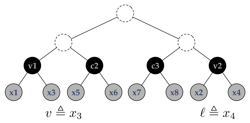
(b) Grafting Lemma 2 Visual Aid.

Figure 6: We reuse the graph in Figure 5(a). The tree in Figure 6(a) is strongly connected and complete. Consider the node $v$. A graft initiated from $v$ may make $v^{\prime\prime}$ a sibling of $v$ because $\texttt{lvs}(v)$ is not a (strict) subset of a connected component and $v^{\prime\prime}$ is maximal. After such a graft, notice that the tree would still satisfy strong connectivity and completeness. The tree in Figure 6(b) is strongly connected but not complete. Consider $x_{3}$ which plays the role of $v$ in the proof of Grafting Lemma 2. When a constrained nearest neighbor search is executed from its parent, $v_{1}$, the leaf $x_{4}$–which plays the role of $\ell$–is returned. If $v_{1}$ and $v_{2}$ are made siblings, their parent is strongly connected.

Lemma 3 (Grafting Lemma 2).

Let ${\mathcal{T}}$ be a tree such that $\texttt{lvs}({\mathcal{T}})=\mathcal{X}$ and let ${\mathcal{T}}$ satisfy strong connectivity. Let $v$ be strongly connected and let $\texttt{lvs}(v)$ be a strict subset of the vertices in some connected component, $C$, in $G$. Then, a graft initiated from $v$ returns a node $v^{\prime}$ such that $v^{\prime}$ is strongly connected and $\texttt{lvs}(v)\subset\texttt{lvs}(v^{\prime})$.

Proof.

Since $\texttt{lvs}(v)$ are a strict subset of the vertices in the connected component, $C$, there exists a non-empty subset $s$ in $\texttt{lvs}({\mathcal{T}})\backslash\texttt{lvs}(v)$ such that $s\cup\texttt{lvs}(v)$ constitute the vertices in $C$. Let $\ell$ maximize $f(v,\ell)$ over all $\texttt{lvs}({\mathcal{T}})\setminus\texttt{lvs}(v)$. By the fact that $\texttt{lvs}(v)$ is a strict subset of a connected component, there must exist an edge between $\texttt{lvs}(v)$ and $\ell$. Note that $\ell$ is the leaf found when the constrained nearest neighbor search from $v$ is initiated in the first line of graft (Algorithm 1).

If $f(v,\ell)<f(\ell,\texttt{s}(\ell))$, then there must exist an edge between $\ell$ and a node in $\texttt{lvs}(\texttt{s}(\ell))$ and so $\texttt{par}(\ell)$ is strongly connected. If $f(v,\ell)<f(v,\texttt{s}(v))$, then there must exist an edge between a node in $\texttt{lvs}(v)$ and a node in $\texttt{lvs}(\texttt{s}(v))$ and so $\texttt{par}(v)$ is strongly connected. In both of these cases, we do not merge $v$ with $\ell$, but instead attempt another merge between two strongly connected nodes, either: $\texttt{par}(v)$ with $\ell$, $v$ with $\texttt{par}(\ell)$, or $\texttt{par}(v)$ with $\texttt{par}(\ell)$. As before, the two nodes we are attempting to merge also have an edge between them.

Let $v_{1}$ and $v_{2}$ be two nodes involved in a merge and let $v_{1}\in\texttt{ancs}(v)$ and $v_{2}\in\texttt{ancs}(\ell)$. If at some point

$$f(v_{1},v_{2})>\max[f(v_{1},\texttt{s}(v_{1})),f(v_{2},\texttt{s}(v_{2}))]$$

then $v_{2}$ is made a sibling of $v_{1}$ and the new parent of $v_{1}$ is returned. Since $v_{1}$ and $v_{2}$ are strongly connected and there exists an edge between $\texttt{lvs}(v_{1})$ and $\texttt{lvs}(v_{2})$, $\texttt{par}(v_{1})$, which is created by the merge, is strongly connected, and the lemma holds.

If a merge is never performed, the recursion stops when $v_{1}=v_{2}=\texttt{lca}(v,\ell)$. In this case, the lca, which we return, is already strongly connected and, by definition, its leaves are a superset of $\texttt{lvs}(v)$. ∎

Lemma 4 (Restructuring Lemma).

Let $v\in{\mathcal{T}}$ be strongly connected. Let $a\in\texttt{ancs}(v)$ be the deepest connected ancestor of $v$ such that: $a$ is not strongly connected, and all siblings of the nodes on the path from $v$ to $a$ are strongly connected. Then restruct on inputs $v$ and $a$ restructures ${\mathcal{T}}[a]$ so that $a$ satisfies strong connectivity.

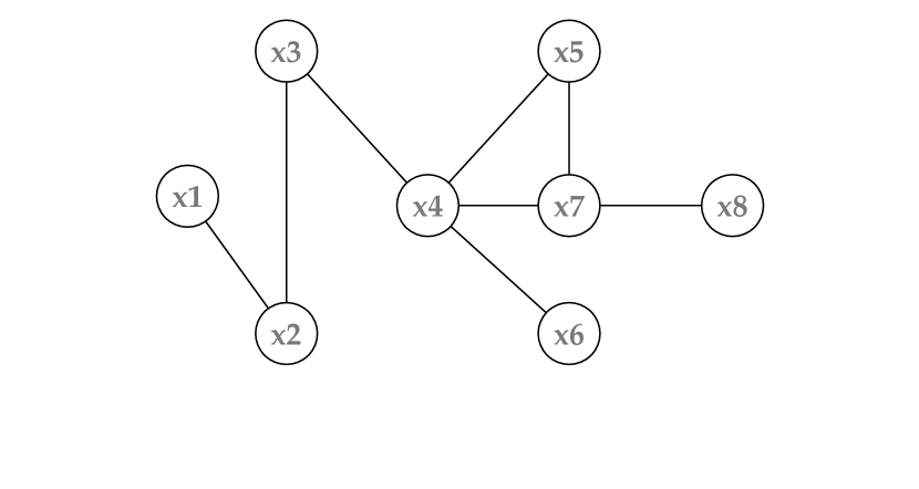
(a) A graph $G=(\mathcal{X},E)$.

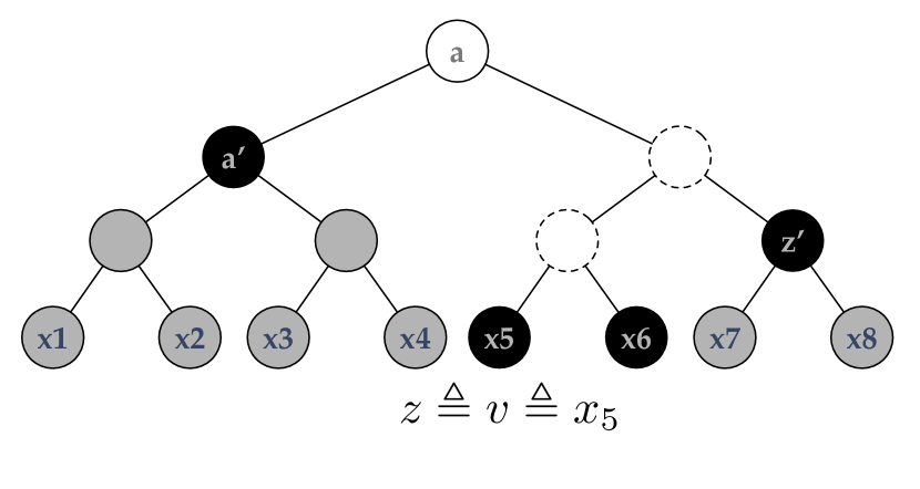
(b) $a$ is connected, but not strongly.

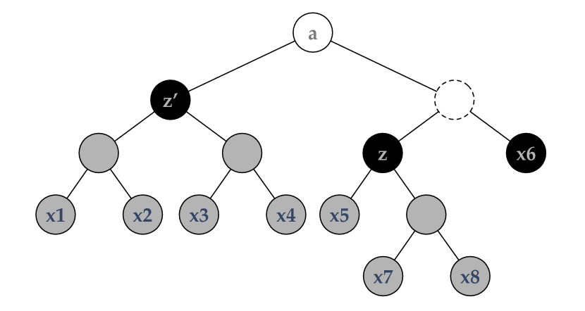
(c) 1 swap applied.

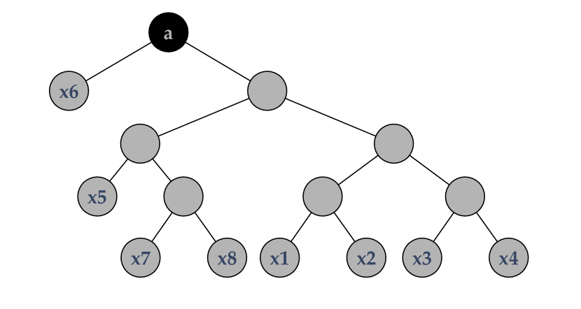
(d) $a$ is strongly connected.

Figure 7: The restruct method. As before, black-filled nodes are maximal, gray-filled nodes are strongly connected, nodes with no fill and solid borders are connected (but not strongly) and nodes with dashed borders are disconnected. Also, note that the labels $z,z^{\prime},\ell$ and $a^{\prime}$ do not apply to the same nodes throughout all figures so to match their usage in proof. In Figure 7(b), $z\triangleq v\triangleq x_{5}$. $\texttt{s}(z)$ and $z^{\prime}$ are swapped to produce the tree in Figure 7(c). Finally, $\texttt{s}(z)$ and $z^{\prime}$ from Figure 7(c) are swapped to produce the tree in Figure 7(d), which is strongly connected.

Proof.

Let $z$ be the deepest ancestor of $v$ that is strongly connected with parent $\texttt{par}(z)$ that is disconnected. Since $\texttt{par}(z)$ is disconnected (but by assumption both $z$ and $\texttt{s}(z)$ are connected), there are no edges between $\texttt{lvs}(z)$ and $\texttt{lvs}(\texttt{s}(z))$.

Let $a^{\prime}$ be a child of $a$ and without loss of generality, $a^{\prime}\not\in\texttt{ancs}(z)$. Since $a$ is the deepest connected ancestor of $z$, there must exist an edge between $\texttt{lvs}(z)$ and $\texttt{lvs}(a^{\prime})$.

When computing the argmax of $f(z,\cdot)$ in the restruct method, a node, $z^{\prime}$, that is connected to $z$ will be returned and then swapped with $\texttt{s}(z)$. The new parent of $z$ is strongly connected because $z$ and $z^{\prime}$ are both strongly connected and there exists an edge between $\texttt{lvs}(z)$ and $\texttt{lvs}(z^{\prime})$. Any subsequent swap attempted from a disconnected node with a connected ancestor succeeds and produces a new parent that is strongly connected.

Since $a$ is connected and a swap among the descendants of $a$ do not change $\texttt{lvs}(a)$, swapping preserves the connectedness of $a$. Therefore, swaps proceed until the node $a$ is reached at which point $a$ must be strongly connected.

Note that a swap attempt between a strongly connected node and a node to which it is not connected fails, because $f$ separates $G$. A swap attempt between a connected node and a node to which it is connected succeeds and produces a new parent that is strongly connected. ∎

We now prove Theorem 1.

Proof.

We show by induction that if Grinch is used to build a tree, ${\mathcal{T}}$, over vertices, $\mathcal{X}$, then the connected components of $G$ are a tree consistent partition in ${\mathcal{T}}$. Furthermore, ${\mathcal{T}}$ satisfies strong connectivity.

Clearly, the theorem holds for the base case: a tree with a single node.

Let $\mathcal{X}=\texttt{lvs}({\mathcal{T}})$. Assume the inductive hypothesis: that ${\mathcal{T}}$ satisfies completeness and strong connectivity. Now vertex $x$ arrives.

If there does not exist an edge between $x$ and any other vertex in $\mathcal{X}$, then after rotations, ${\mathcal{T}}^{\prime}$ satisfies completeness. Since $\forall a\in\texttt{ancs}(x)$, $\texttt{lvs}(a)$ is a not a strict subset of any connected component in $G$, by Grafting Lemma 1, subsequent graft attempts from the ancestors of $x$ preserve strong connectivity and completeness and so the theorem holds.

Assume that $x$ is connected to some set of leaves $s\subseteq\texttt{lvs}({\mathcal{T}})$. Since ${\mathcal{T}}$ satisfies strong connectivity, by the Rotation Lemma, after $x$ is added and rotations terminate, ${\mathcal{T}}^{\prime}$ satisfies strong connectivity. Note that ${\mathcal{T}}^{\prime}$ may not satisfy completeness if, before the arrival of $x$, the leaves in $s$ formed at least 2 distinct connected subgraphs in $G$.

After rotations, a series of graft attempts are performed. Consider the first graft initiated at $\texttt{par}(x)$. By Grafting Lemma 2, the attempt returns a strongly connected ancestor of $x$ whose leaves are a strict superset of $\texttt{lvs}(x)$. If a merge is performed that moves a node $v$ and makes it a sibling of $v^{\prime}$, then strong connectivity may be violated. However, notice that the only nodes that can be disconnected by such a merge are the node that, prior to the merge, were ancestors of $v$ and also descendants of $a=\texttt{lca}(v,v^{\prime})$.

After the merge, $a$ is restructured, and by the Restructuring Lemma, the resulting tree satisfies strong connectivity. Subsequent calls to graft proceed from $a$. Notice that each invocation of graft returns a new strongly connected node with a strictly larger number of descendant leaves, until the resulting tree satisfies completeness. Therefore, successive grafting followed by restructuring eventually returns a node whose leaves are a connected component of $G$. Ultimately, after rotations and grafting, ${\mathcal{T}}^{\prime}$ must satisfy completeness and strong connectivity. ∎

References

- [1]
- dbl [[n. d.]] [n. d.]. DBLP Disambiguation Page for: Wei Wang. https://dblp.uni-trier.de/pers/hd/w/Wang:Wei. Accessed: 2018-05-17.
- Balcan et al. [2008] M.-F. Balcan, A. Blum, and S. Vempala. 2008. A discriminative framework for clustering via similarity functions. In Symposium on Theory of computing.
- Bateni et al. [2017] M. Bateni, S. Behnezhad, M. Derakhshan, M. Hajiaghayi, R. Kiveris, S. Lattanzi, and V. Mirrokni. 2017. Affinity Clustering: Hierarchical Clustering at Scale. In Advances in Neural Information Processing Systems.
- Blundell and Teh [2013] C. Blundell and Y. W. Teh. 2013. Bayesian hierarchical community discovery. In Advances in Neural Information Processing Systems.
- Blundell et al. [2011] C. Blundell, Y. W. Teh, and K. A. Heller. 2011. Discovering non-binary hierarchical structures with Bayesian rose trees. Mixture Estimation and Applications. John Wiley & Sons (2011).
- Clark and Manning [2016] K. Clark and C. D. Manning. 2016. Improving Coreference Resolution by Learning Entity-Level Distributed Representations. In Association for Computational Linguistics.
- Cohen-Addad et al. [2018] Vincent Cohen-Addad, Varun Kanade, Frederik Mallmann-Trenn, and Claire Mathieu. 2018. Hierarchical clustering: Objective functions and algorithms. In Symposium on Discrete Algorithms.
- Culotta et al. [2007] A. Culotta, P. Kanani, R. Hall, M. Wick, and A. McCallum. 2007. Author disambiguation using error-driven machine learning with a ranking loss function. In Workshop on Information Integration on the Web.
- Dasgupta [2015] S. Dasgupta. 2015. A cost function for similarity-based hierarchical clustering. arXiv:1510.05043 (2015).
- Eisen et al. [1998] M. B. Eisen, P. T. Spellman, P. O. Brown, and D. Botstein. 1998. Cluster analysis and display of genome-wide expression patterns. Proceedings of the National Academy of Sciences (1998).
- Ester et al. [1996] M. Ester, H. Kriegel, J. Sander, X. Xu, et al. 1996. A density-based algorithm for discovering clusters in large spatial databases with noise.. In KDD.
- Geusebroek et al. [2005] J. Geusebroek, G. J. Burghouts, and A. W.M. Smeulders. 2005. The Amsterdam library of object images. International Journal of Computer Vision (2005).
- Greenberg et al. [2014] C. S. Greenberg, D. Bansé, G. R. Doddington, D. Garcia-Romero, J. J. Godfrey, T. Kinnunen, A. F. Martin, A. McCree, M. Przybocki, and D. A. Reynolds. 2014. The NIST 2014 speaker recognition i-vector machine learning challenge. In Odyssey: The Speaker and Language Recognition Workshop.
- Haghighi and Klein [2010] A. Haghighi and D. Klein. 2010. Coreference resolution in a modular, entity-centered model. In Human Language Technologies: Association for Computational Linguistics.
- Han et al. [2005] H. Han, H. Zha, and C. L. Giles. 2005. Name disambiguation in author citations using a k-way spectral clustering method. In Joint Conference on Digital Libraries.
- Heller and Ghahramani [2005a] K. Heller and Z. Ghahramani. 2005a. Randomized algorithms for fast Bayesian hierarchical clustering. (2005).
- Heller and Ghahramani [2005b] K. A. Heller and Z. Ghahramani. 2005b. Bayesian hierarchical clustering. In International conference on Machine Learning.
- Jain and Neal [2004] S. Jain and R. M. Neal. 2004. A split-merge Markov chain Monte Carlo procedure for the Dirichlet process mixture model. Journal of computational and Graphical Statistics (2004).
- Kleinberg [2000] J. Kleinberg. 2000. The small-world phenomenon: An algorithmic perspective. In Symposium on Theory of computing.
- Kleinberg [2006] J. Kleinberg. 2006. Complex networks and decentralized search algorithms. In International Congress of Mathematicians (ICM).
- Kobren et al. [2017] A. Kobren, N. Monath, A. Krishnamurthy, and A. McCallum. 2017. A Hierarchical Algorithm for Extreme Clustering. KDD (2017).
- Kohli et al. [2009] Pushmeet Kohli, Philip HS Torr, et al. 2009. Robust higher order potentials for enforcing label consistency. International Journal of Computer Vision (2009).
- Krishnamurthy et al. [2012] A. Krishnamurthy, S. Balakrishnan, M. Xu, and A. Singh. 2012. Efficient active algorithms for hierarchical clustering. International Conference on Machine Learning (2012).
- Lee et al. [2012] H. Lee, M. Recasens, A. Chang, M. Surdeanu, and D. Jurafsky. 2012. Joint entity and event coreference resolution across documents. In Joint Conference on Empirical Methods in Natural Language Processing and Computational Natural Language Learning.
- Liberty et al. [2016] E. Liberty, R. Sriharsha, and M. Sviridenko. 2016. An algorithm for online k-means clustering. In Workshop on Algorithm Engineering and Experiments.
- Malkov et al. [2014] Y. Malkov, A. Ponomarenko, A. Logvinov, and V. Krylov. 2014. Approximate nearest neighbor algorithm based on navigable small world graphs. Information Systems (2014).
- Russakovsky et al. [2015] O. Russakovsky, J. Deng, H. Su, J. Krause, S. Satheesh, S. Ma, Z. Huang, A. Karpathy, A. Khosla, M. Bernstein, et al. 2015. Imagenet large scale visual recognition challenge. International Journal of Computer Vision (2015).
- Singh et al. [2011] S. Singh, A. Subramanya, F. Pereira, and A. McCallum. 2011. Large-scale cross-document coreference using distributed inference and hierarchical models. In Association for Computational Linguistics: Human Language Technologies.
- Wang and Wang [2018] Dingkang Wang and Yusu Wang. 2018. An Improved Cost Function for Hierarchical Cluster Trees. CoRR (2018).
- Watts and Strogatz [1998] D. J. Watts and S. H. Strogatz. 1998. Collective dynamics of ‘small-world’networks. Nature (1998).
- Wick et al. [2012] M. Wick, S. Singh, and A. McCallum. 2012. A discriminative hierarchical model for fast coreference at large scale. In Association for Computational Linguistics.
- Wiseman et al. [2016] S. Wiseman, A. M. Rush, and S. M Shieber. 2016. Learning global features for coreference resolution. NAACL-HLT (2016).
- Zhang et al. [2013] L. Zhang, M. Song, Z. Liu, X. Liu, J. Bu, and C. Chen. 2013. Probabilistic graphlet cut: Exploiting spatial structure cue for weakly supervised image segmentation. In Computer Vision and Pattern Recognition. IEEE.
- Zhang et al. [1996] T. Zhang, R. Ramakrishnan, and M. Livny. 1996. BIRCH: an efficient data clustering method for very large databases. In ACM Sigmod Record.