Bound states in two-dimensional Fermi systems with quadratic band touching

Abstract

The formation of bound states between mobile impurity particles and fermionic atoms has been demonstrated in spin-polarized Fermi gases with attractive interspecies interaction. We investigate bound states of mobile impurities immersed in a two-dimensional system with a symmetry-protected quadratic band touching. In addition to the standard $s$-wave interaction, we consider an anisotropic dipolar exchange interaction that locally breaks point group symmetries. Using a weak-coupling renormalization group approach and a ladder approximation for the impurity-fermion propagator, we establish that the number of bound states can be controlled by varying the anisotropy of the exchange interaction. Our results show that the degeneracy and momentum dependence of the binding energies reflect some distinctive properties of the quadratic band touching.

I Introduction

Topological semimetals with quadratic band touching (QBT) in two dimensions constitute examples of gapless band structures protected by point group and time reversal symmetries Fradkin (2013); Sun et al. (2009). Microscopic models exhibiting QBT have been proposed and studied on the checkerboard and kagome lattices Sun et al. (2009); Liu et al. (2010); Uebelacker and Honerkamp (2011); Dóra et al. (2014). Unlike Dirac points in graphene, two-dimensional QBT points have a nonvanishing density of states and their effective action is scale invariant with dynamical exponent $z=2$ Fradkin (2013). This makes the QBT unstable against weak short-range interactions and leads to phase transitions where at least one symmetry is spontaneously broken. As a consequence, anomalous quantum Hall and nematic semimetal phases were predicted based on a perturbative renormalization group (RG) approach and mean-field theory Sun et al. (2009), and were recently investigated in numerical studies Sur et al. (2018); Zeng et al. (2018). Experimental realizations of QBT systems in optical lattices have also been discussed Ölschläger et al. (2012); Sun et al. (2012); Li and Liu (2016).

In this work we consider a (pseudo-)spin-$1/2$ fermionic model where a single spin-down fermion interacts with a QBT system of majority, spin-up fermions. This limit of extreme population imbalance has received considerable attention in the context of cold atomic realizations of Fermi polarons Massignan et al. (2014); Zöllner et al. (2011); Mathy et al. (2011); Parish (2011); Klawunn and Recati (2011); Schmidt et al. (2012), where mobile impurity atoms are dressed by particle-hole excitations of the Fermi gas in which they are immersed. The quasiparticle properties of Fermi polarons have been measured using radio-frequency spectroscopy Schirotzek et al. (2009); Koschorreck et al. (2012); Kohstall et al. (2012); Scazza et al. (2017). Beyond the conventional polaron picture, mobile impurities can probe exotic properties of many-body systems such as topological phase transitions Grusdt et al. (2016); Camacho-Guardian et al. (2019); Qin et al. (2019); Grusdt et al. (2019) and quasiparticle breakdown associated with quantum criticality Caracanhas et al. (2013); Punk and Sachdev (2013); Caracanhas and Pereira (2016); Yan et al. (2019).

In Ref. Caracanhas and Pereira (2016), the fate of a polaron in a QBT system was shown to depend on the particle-hole asymmetry of the band structure. If the effective mass of the upper band (above the QBT point) is larger than that of the lower band, a repulsive $s$-wave impurity-fermion interaction decreases logarithmically with decreasing energy scale, giving rise to a marginal Fermi polaron. On the other hand, if the lower band has larger effective mass, the effective interaction increases at low energies, driving the quasiparticle weight to zero and bringing about an emergent orthogonality catastrophe Caracanhas and Pereira (2016).

The purpose of this paper is twofold: First, we generalize the model of Ref. Caracanhas and Pereira (2016) to include a long-range spin exchange interaction between the mobile impurity and the majority fermions. The motivation comes from dipolar quantum gases Lahaye et al. (2009), in which spin exchange has been demonstrated experimentally Yan et al. (2013); Hazzard et al. (2014). In these systems, the spatial anisotropy of the dipolar interaction can be controlled by varying the direction of the molecular electric dipole moments. We show that in the low-energy limit the anisotropic spin exchange generates an impurity-fermion interaction that locally breaks point group symmetries. This modifies the renormalization group flow of the effective couplings in the quantum impurity model. We find a regime in which a bare repulsive interaction becomes effectively attractive at low energies. Second, we study the formation of bound states in analogy with the corresponding phenomenon in two-dimensional Fermi gases with attractive interactions Zöllner et al. (2011); Mathy et al. (2011); Parish (2011); Klawunn and Recati (2011); Schmidt et al. (2012). We find that the spectrum of an impurity coupled to a QBT system can exhibit zero, one or two bound states depending on the relative strength of the $s$-wave contact interaction and the symmetry-breaking interaction due to anisotropic exchange. In particular, for an attractive $s$-wave interaction and no anisotropic exchange, there are two bound states which become degenerate for vanishing total momentum. Turning on a small anisotropic interaction, the degeneracy point can move to finite momenta along specific directions determined by the QBT Hamiltonian.

The remainder of the paper is organized as follows: In Sec. II, we present the microscopic model on the checkerboard lattice and the effective field theory in the continuum limit. In Sec. III, we analyze the interacting model using a perturbative RG approach, which reveals the existence of a crossover regime where the effective coupling changes sign. In Sec. IV, we calculate the two-particle propagator and the associated pair spectral function in the ladder approximation, and discuss the different regimes for the formation of bound states. Our concluding remarks can be found in Sec. V. The Appendix contains expressions for functions that appear in the RG equations and some discussion about the two-body problem with one particle near the QBT.

II Model

We start with the model

$$H = -\sum_{\langle ij\rangle}t_{ij}(c^{\dagger}_{i\uparrow}c^{\phantom{\dagger}}_{j\uparrow}+c^{\dagger}_{i\downarrow}c^{\phantom{\dagger}}_{j\downarrow})+U\sum_{i}n_{i\uparrow}n_{i\downarrow}$$ (1)

$$+\frac{J_{\perp}}{4}\sum_{i\neq j}V_{ij}(S_{i}^{+}S_{j}^{-}+S_{i}^{-}S_{j}^{+}).$$

Here, $c^{\dagger}_{j\alpha}$ creates a fermion at site $j$ in one of two internal states, labeled by $\alpha=\uparrow,\downarrow$, and $n_{j\alpha}=c^{\dagger}_{j\alpha}c^{\phantom{\dagger}}_{j\alpha}$. The hopping parameters $t_{ij}$ are defined on the checkerboard lattice. While the nearest-neighbor hopping $t$ is uniform, the next-nearest-neighbor hopping is either $t^{\prime}$ or $t^{\prime\prime}$ depending on the sublattice and the direction of the link, as illustrated in Fig. 1. For two next-nearest-neighbor sites in the A (B) sublattice, the hopping parameter is $t^{\prime}$ along the $x$ ($y$) direction, but $t^{\prime\prime}$ along the $y$ ($x$) direction. In addition to the on-site Hubbard repulsion $U>0$, we consider a dipolar exchange interaction Gorshkov et al. (2011); Zou et al. (2017) written in terms of spin operators $S_{j}^{+}=c^{\dagger}_{j\uparrow}c^{\phantom{\dagger}}_{j\downarrow}$ and $S_{j}^{-}=c^{\dagger}_{j\downarrow}c^{\phantom{\dagger}}_{j\uparrow}$. The geometrical factor

$$V_{ij}=\frac{1-3(\hat{\mathbf{d}}\cdot\hat{\mathbf{r}}_{ij})^{2}}{|\mathbf{r}_{ij}|^{3}}$$ (2)

depends on the relative position $\mathbf{r}_{ij}=\mathbf{r}_{i}-\mathbf{r}_{j}$ between sites. Here $\hat{\mathbf{d}}$ is a unit vector parallel to the quantization axis, set by the direction of the polarized dipole moments Gorshkov et al. (2011). This type of exchange interaction was realized using two rotational states of polar molecules in optical lattices Yan et al. (2013). In terms of the angles shown in Fig. 1, we can write $\hat{\mathbf{d}}\cdot\hat{\mathbf{r}}_{ij}=\sin\theta\cos(\phi-\varphi_{ij})$, where $\theta$ and $\phi$ are the angles of the $\mathbf{d}$ vector and $\varphi_{ij}$ is the angle between $\mathbf{r}_{ij}$ and the $x$ axis. Note that for $\theta\neq 0,\pi$ the strength of the dipolar exchange interaction depends on the direction of $\mathbf{r}_{ij}$.

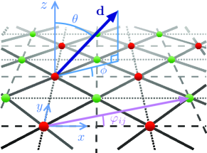
Figure 1: Checkerboard lattice. Solid lines represent the nearest-neighbor hopping $t$ between sites in sublattice A (red) and B (green). Dashed and dotted lines represent next-nearest-neighbor hopping $t^{\prime}$ and $t^{\prime\prime}$, respectively. The spin exchange interaction depends on the direction of the dipolar moment $\mathbf{d}$, parametrized by the polar angle $\theta$ (with respect to the $z$ axis, perpendicular to the lattice plane) and the azimuthal angle $\phi$ (measured from the $x$ axis). A vector $\mathbf{r}_{ij}$ connecting two lattice sites forms an angle $\varphi_{ij}$ with the $x$ axis.

In the noninteracting case, $U=J_{\perp}=0$, we can diagonalize the Hamiltonian using the mode expansion

$$c_{j\alpha} = \left\{\begin{array}[]{ll}\frac{1}{\sqrt{N_{s}}}\sum_{\mathbf{k}}a_{\mathbf{k}\alpha}e^{i\mathbf{k}\cdot\mathbf{R}_{j}},&\quad j\in\textrm{A}\\ \frac{1}{\sqrt{N_{s}}}\sum_{\mathbf{k}}b_{\mathbf{k}\alpha}e^{i\mathbf{k}\cdot(\mathbf{R}_{j}+\bm{\delta})},&\quad j\in\textrm{B}\end{array}\right.,$$ (5)

where $\mathbf{R}_{j}$ are positions on the square lattice with lattice spacing set equal to $1$, $N_{s}$ is the number of unit cells of the checkerboard lattice, and $\bm{\delta}=(\hat{\mathbf{x}}+\hat{\mathbf{y}})/2$ connects two sites in the same unit cell. The noninteracting Hamiltonian has the form $H_{0}=\sum_{\mathbf{k},\alpha}c^{\dagger}_{\mathbf{k}\alpha}\mathcal{H}_{0}(\mathbf{k})c^{\phantom{\dagger}}_{\mathbf{k}\alpha}$, with

$$\mathcal{H}_{0}(\mathbf{k}) = -(t^{\prime}+t^{\prime\prime})(\cos k_{x}+\cos k_{y})\openone$$ (6)

$$-(t^{\prime}-t^{\prime\prime})(\cos k_{x}-\cos k_{y})\sigma^{z}$$

$$-4t\cos(k_{x}/2)\cos(k_{y}/2)\sigma^{x}.$$

Here $c_{\mathbf{k}\alpha}=(a_{\mathbf{k}\alpha},b_{\mathbf{k}\alpha})$ is a two-component spinor and $\sigma^{x},\sigma^{y},\sigma^{z}$ are Pauli matrices acting in the sublattice space. The noninteracting Hamiltonian has a C₄ rotational symmetry corresponding to $\sigma^{y}\mathcal{H}_{0}(k_{x},k_{y})\sigma^{y}=\mathcal{H}_{0}(k_{y},2\pi-k_{x})$. In addition, $H_{0}$ is invariant under complex conjugation, equivalent to time reversal in sectors of the Fock space with fixed $N_{\uparrow}=\sum_{j}c^{\dagger}_{j\uparrow}c^{\phantom{\dagger}}_{j\uparrow}$ and $N_{\downarrow}=\sum_{j}c^{\dagger}_{j\downarrow}c^{\phantom{\dagger}}_{j\downarrow}$. For $|t^{\prime}+t^{\prime\prime}|<|t|$ and $|t^{\prime}+t^{\prime\prime}|<|t^{\prime}-t^{\prime\prime}|$, the band structure has a QBT point at the corner of the Brillouin zone, $\mathbf{Q}=(\pi,\pi)$ Sun et al. (2009), as illustrated in Fig. 2. This QBT point does not require fine tuning, since it carries Berry phase $\pm 2\pi$ and is protected by C₄ and time reversal symmetries.

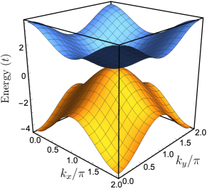
Figure 2: Band structure for the noninteracting checkerboard lattice model showing the quadratic band touching at $\mathbf{Q}=(\pi,\pi)$. Here we set $t^{\prime}=0.6t$ and $t^{\prime\prime}=-0.4t$.

Let us focus on the single-impurity model with $N_{\uparrow}=N_{s}$ and $N_{\downarrow}=1$ in the thermodynamic limit $N_{s}\to\infty$. In this case, the Fermi level of the spin-up (majority) fermions lies at the QBT point. We can describe their low-energy excitations by expanding around momentum $\mathbf{Q}$. Hereafter we assume $t^{\prime\prime}<0$ and $t=t^{\prime}-t^{\prime\prime}>0$, in which case the dispersion around the QBT point becomes isotropic in the continuum limit Sun et al. (2009); Caracanhas and Pereira (2016). By contrast, the low-energy limit for the impurity is obtained by expanding around the bottom of the lower band, at $\mathbf{k}=0$. The non-interacting Hamiltonian in the continuum limit becomes, up to a constant,

$$H_{0}=\int d^{2}r\left[\Psi^{\dagger}(\mathbf{r})h_{0}(\mathbf{r})\Psi(\mathbf{r})-d^{\dagger}(\mathbf{r})\frac{\nabla^{2}}{2M}d(\mathbf{r})\right],$$ (7)

where $\Psi(\mathbf{r})=(\psi_{A}(\mathbf{r}),\psi_{B}(\mathbf{r}))^{t}$ is the two-component spinor associated with the majority fermions and $d(\mathbf{r})$ is the mobile impurity field with effective mass $M=(2t^{\prime})^{-1}$. The operator

$$h_{0}(\mathbf{r}) = \frac{m_{+}-m_{-}}{4m_{+}m_{-}}\openone\nabla^{2}+$$ (8)

$$+\frac{m_{+}+m_{-}}{4m_{+}m_{-}}\left[\sigma^{z}(\partial_{x}^{2}-\partial_{y}^{2})+2\sigma^{x}\partial_{x}\partial_{y}\right]$$

involves the effective masses in the vicinity of the QBT point: $m_{+}=[2(t-t^{\prime})]^{-1}$ and $m_{-}=(2t^{\prime})^{-1}$ for the upper and lower bands, respectively.

We now switch on the interactions in the weak coupling regime $U,|J_{\perp}|\ll t$. The interacting Hamiltonian in the continuum limit has the form $H=H_{0}+H_{int}$, with $H_{0}$ given in Eq. (7) and the impurity-fermion interaction given by

$$H_{int}=\frac{4\pi}{m_{+}}\int d^{2}r\,\Psi^{\dagger}(\mathbf{r})(g\openone+g_{\perp}\sigma^{x})\Psi(\mathbf{r})d^{\dagger}(\mathbf{r})d(\mathbf{r}),$$ (9)

where we define the dimensionless couplings

$$g = \frac{m_{+}}{8\pi}\left[U-\kappa J_{\perp}\left(\frac{3}{2}\sin^{2}\theta-1\right)\right],$$

$$g_{\perp} = -\frac{3m_{+}}{4\pi}\kappa_{\perp}J_{\perp}\sin^{2}\theta\sin(2\phi).$$ (10)

The latter stem from the Fourier transform of the on-site and dipolar exchange interactions and contain the constants

$$\kappa = \frac{3}{2}\zeta(3)-2\sum_{m=1}^{\infty}\sum_{n=1}^{\infty}\frac{(-1)^{m+n}}{(m^{2}+n^{2})^{3/2}}\approx 1.322,$$ (11)

$$\kappa_{\perp} = \sum_{m=0}^{\infty}\sum_{n=0}^{\infty}\frac{(-1)^{m+n}\left(m+\frac{1}{2}\right)\left(n+\frac{1}{2}\right)}{\left[\left(m+\frac{1}{2}\right)^{2}+\left(n+\frac{1}{2}\right)^{2}\right]^{5/2}}\approx 1.312,$$

where $\zeta(s)$ is the Riemann zeta function.

We interpret $g$ in Eq. (9) as the usual $s$-wave scattering amplitude between the impurity and the majority fermions, whereas the new interaction $g_{\perp}$ scatters fermions between different sublattice states. Note that $g_{\perp}$ depends on the spatial anisotropy of the exchange interaction, and it vanishes when the dipolar moment is polarized along the $z$ axis. In fact, the $g_{\perp}$ interaction breaks the C₄ symmetry, which in the continuum limit becomes $\Psi(x,y)\mapsto\sigma^{y}\Psi(y,-x)$. Importantly, both $g$ and $g_{\perp}$ are local interactions at the position of the mobile impurity and there are no interactions between majority fermions in the bulk. Thus, the single-impurity model allows us to explore the effects of a local symmetry-breaking interaction without destabilizing the QBT.

III Renormalization group analysis

Short-range interactions are known to be marginal perturbations of two-dimensional semimetals with a QBT Sun et al. (2009); Murray and Vafek (2014); Caracanhas and Pereira (2016). To treat the interactions within perturbation theory, we introduce the impurity Green’s function

$$G_{d}(\mathbf{r},\tau)=-\langle T_{\tau}d(\mathbf{r},\tau)d^{\dagger}(\mathbf{0},0)\rangle,$$ (12)

where $d(\mathbf{r},\tau)=e^{H\tau}d(\mathbf{r})e^{-H\tau}$ is the impurity field evolved in imaginary time, $T_{\tau}$ denotes time ordering with respect to $\tau$, and the expectation value is calculated in the ground state with $N_{\downarrow}=0$. To zeroth order in the interactions, we have the noninteracting Green’s function in momentum-frequency domain:

$$G^{(0)}_{d}(\mathbf{k},i\nu)=\frac{1}{i\nu-k^{2}/(2M)}.$$ (13)

For the majority fermions, we define the matrix Green’s function

$$\mathbbm{G}=\left(\begin{array}[]{cc}\mathcal{G}_{AA}&\mathcal{G}_{AB}\\ \mathcal{G}_{BA}&\mathcal{G}_{BB}\end{array}\right),$$ (14)

with components

$$\mathcal{G}_{ll^{\prime}}(\mathbf{r},\tau)=-\langle T_{\tau}\psi^{\phantom{\dagger}}_{l}(\mathbf{r},\tau)\psi^{\dagger}_{l^{\prime}}(\mathbf{0},0)\rangle,$$ (15)

where $l=A,B$ is the sublattice index. The Fourier-transformed noninteracting Green’s function reads

$$\mathcal{G}^{(0)}_{ll^{\prime}}(\mathbf{p},i\nu) = \left\{[i\omega\openone-\mathcal{H}_{0}(\mathbf{Q}+\mathbf{p})]^{-1}\right\}_{ll^{\prime}}$$ (16)

$$= \sum_{\lambda=\pm}\frac{U_{l\lambda}(\mathbf{p})U_{l^{\prime}\lambda}(\mathbf{p})}{i\nu-\lambda p^{2}/(2m_{\lambda})}.$$

Here $U_{l\lambda}(\mathbf{p})$, with $\lambda=\pm$ the band index, are the matrix elements of the unitary transformation that diagonalizes $h_{0}(\mathbf{p})=\mathcal{H}_{0}(\mathbf{Q}+\mathbf{p})$ with $|\mathbf{p}|\ll 1$. Due to the Berry phase associated with the QBT, $U(\mathbf{p})$ depends on the angle $\varphi_{\mathbf{p}}=\arctan(p_{y}/p_{x})$, in the form

$$U(\mathbf{p})=U(\varphi_{\mathbf{p}})=\left(\begin{array}[]{cc}\sin\varphi_{\mathbf{p}}&\cos\varphi_{\mathbf{p}}\\ -\cos\varphi_{\mathbf{p}}&\sin\varphi_{\mathbf{p}}\end{array}\right).$$ (17)

We analyze the effects of the impurity-fermion interaction using a weak-coupling Wilsonian RG approach Shankar (1994); Cardy et al. (1996). We derive the RG equations for the coupling constants at one-loop level and for the impurity effective mass and quasiparticle weight at two-loop level by integrating out high-energy fermion states in the momentum shell $\Lambda(1-d\ell)<p^{2}/(2m_{+})<\Lambda$, where $\Lambda$ is the ultraviolet cutoff and $d\ell\ll 1$ is the infinitesimal parameter in the RG step. For instance, the diagrams that contribute to the renormalization of the interaction vertex are shown in Fig. 3. We obtain the set of coupled RG equations:

$$\frac{dg}{d\ell} = \frac{\left(\mu_{-}-\mu_{+}\right)Z_{d}}{m_{+}}(g^{2}+g_{\perp}^{2}),\$$

$$\frac{dg_{\perp}}{d\ell} = \frac{2(\mu_{-}-\mu_{+})Z_{d}}{m_{+}}gg_{\perp},$$ (18)

$$\frac{dZ_{d}}{d\ell} = -\frac{2\mu_{-}\mu_{+}Z_{d}}{m_{+}}\left[g^{2}F_{1}(r_{+},r_{-})+g_{\perp}^{2}F_{2}(r_{+},r_{-})\right],$$

$$\frac{dM}{d\ell} = \frac{2(\mu_{-}\mu_{+})^{3/2}}{m_{+}}\left[g^{2}F_{3}(r_{+},r_{-})+g_{\perp}^{2}F_{4}(r_{+},r_{-})\right],$$

where $Z_{d}$ is the impurity quasiparticle weight, $\mu_{\pm}=m_{\pm}M/(M+m_{\pm})$ are reduced masses, and $r_{\pm}=m_{\pm}/M$ are mass ratios. The functions $F_{i}(r_{+},r_{-})$, with $i=1,\dots,4$, are given in terms of integrals in Appendix A and return positive values of order 1. Note that bulk properties, such as the effective masses $m_{+}$ and $m_{-}$ for the majority fermions, are not renormalized in the single-impurity problem.

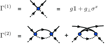
Figure 3: Effective interaction vertex at tree level ($\Gamma^{(1)}$) and at one-loop level ($\Gamma^{(2)}$). Solid lines represent the bare propagator for majority fermions, while dashed lines represent the impurity propagator. The matrices in the interaction vertex act on the fermion sublattice degree of freedom.

The case $g>0$ and $g_{\perp}=0$ was studied in Ref. Caracanhas and Pereira (2016). In this case, $g$ can be marginally relevant or irrelevant depending on the difference between the effective masses $m_{+}$ and $m_{-}$. The reason is that the two one-loop diagrams in the vertex renormalization (see Fig. 3) have opposite signs. For $m_{-}>m_{+}$, the diagram with a hole propagator in the loop dominates and the repulsive impurity-fermion interaction flows to strong coupling. Ultimately, the quasiparticle weight $Z_{d}$ vanishes and the effective impurity mass $M$ diverges logarithmically in the low-energy limit Caracanhas and Pereira (2016).

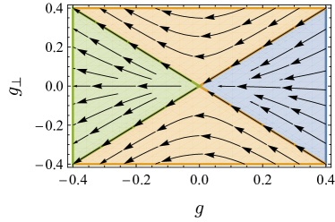
Figure 4: Renormalization group flow of the couplings in the single-impurity model with $m_{-}<m_{+}$. In the crossover region $|g|<|g_{\perp}|$ (orange), an initially repulsive $s$-wave scattering amplitude $g>0$ can change sign and become attractive.

Here we are interested in the case $m_{-}<m_{+}$, in which the diagram with a fermionic particle propagator in the loop dominates the vertex renormalization. The RG flow diagram for the couplings $g$ and $g_{\perp}$ in Fig. 4 reveals three regions with qualitatively different behavior. For $|g_{\perp}|<g$ (blue region in Fig. 4), the interaction is marginally irrelevant. As a result, in the low-energy limit the impurity decouples from the fermionic bath and one recovers Fermi polaron behavior with logarithmic corrections Caracanhas and Pereira (2016). When we start off with an attractive interaction in the regime $g<-|g_{\perp}|$ (green region in Fig. 4), the system exhibits monotonic flow to strong coupling. Finally and most remarkably, for $|g|<|g_{\perp}|$ (orange region in Fig. 4), we observe a crossover from weak repulsive interaction to strong attractive interaction, $g<0$. Our goal in the following will be to analyze the fate of the impurity in the latter two regions.

IV Pair spectral function

The flow of the effective couplings to strong attraction signals the formation of bound states between the impurity and a majority fermion. In two dimensions, at least one bound state exists in the two-body problem for an arbitrarily weak attractive interaction Mathy et al. (2011); Parish (2011); Klawunn and Recati (2011); Schmidt et al. (2012). To investigate the presence of bound states, we consider the pair creation operator

$$P^{\dagger}(\mathbf{r}_{j})=c^{\dagger}_{j\uparrow}c^{\dagger}_{j\downarrow}.$$ (19)

We then define the two-particle propagator as a matrix in sublattice space, with components

$$\Pi_{ll^{\prime}}(\mathbf{R},\tau) = -(-1)^{s_{l}+s_{l^{\prime}}}2\langle T_{\tau}P(\mathbf{R}+s_{l}\bm{\delta},\tau)P^{\dagger}(s_{l^{\prime}}\bm{\delta},0)\rangle,$$

where $\mathbf{R}$ is a position vector in sublattice A and $s_{A}=0$, $s_{B}=1$. At low energies, we can work with the two-particle propagator in the continuum limit:

$$\Pi_{ll^{\prime}}(\mathbf{r},\tau)=-\langle T_{\tau}\psi_{l}^{\phantom{\dagger}}(\mathbf{r},\tau)d(\mathbf{r},\tau)d^{\dagger}(\mathbf{0},0)\psi_{l^{\prime}}^{\dagger}(\mathbf{0},0)\rangle,$$ (21)

where the factor of $(-1)^{s_{l}+s_{l^{\prime}}}2$ in Eq. (LABEL:2pprop) gets cancelled in the projection of $c_{j\downarrow}$ onto the impurity field. Taking the Fourier transform,

$$\Pi_{ll^{\prime}}(\mathbf{q},i\omega)=\int d^{2}rd\tau\,e^{i\omega\tau}e^{-i\mathbf{q}\cdot\mathbf{r}}\,\Pi_{ll^{\prime}}(\mathbf{r},\tau),$$ (22)

and the analytic continuation $i\omega\to\omega+i0^{+}$, we define the pair spectral function

$$\mathcal{A}_{\textrm{pair}}(\mathbf{q},\omega)=-2\textrm{Im}\{\textrm{Tr}[\Pi(\mathbf{q},\omega+i0^{+})]\}.$$ (23)

When interpreting the result for $\mathcal{A}_{\textrm{pair}}(\mathbf{q},\omega)$ in the continuum limit in terms of the original lattice model, we must recall that zero energy corresponds to the impurity at the bottom of the lower band and the spin-up fermion at the QBT point.

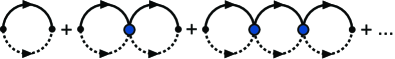
Figure 5: Feynman diagrams included in the ladder approximation for the two-particle propagator. The convention for the interaction vextex and for impurity and fermion propagators is the same as in Fig. 3.

We calculate the two-particle propagator in the ladder approximation Mahan (2000); Massignan et al. (2014). This approximation is justified because, according to the RG analysis in Sec. III, for $m_{-}<m_{+}$ the perturbative expansion is dominated by diagrams with a particle propagator in the loops. The ladder series is illustrated in Fig. 5. The diagrams involve the bare two-particle propagator

$$\Pi_{0}(\mathbf{q},i\omega) = \int\frac{d^{2}pd\nu}{(2\pi)^{3}}\mathbb{G}^{(0)}(\mathbf{p}+\mathbf{q},i\omega+i\nu)G^{(0)}_{d}(-\mathbf{p},-i\nu)$$ (24)

$$= \frac{\mu_{+}}{4\pi}\left\{\log\left(\frac{W-i\omega}{\Omega(q)-i\omega}\right)\openone\right.$$

$$-\left[1+\frac{Mq^{2}-2iM^{2}\omega}{\mu_{+}q^{2}}\log\left(\frac{i\omega-\Omega(q)}{i\omega-\frac{q^{2}}{2M}}\right)\right]$$

$$\times\left[\cos{(2\varphi_{\mathbf{q}})}\sigma^{z}+\sin{(2\varphi_{\mathbf{q}})}\sigma^{x}\right]\Big{\}},$$

where $W$ is a high-energy cutoff and $\Omega(q)=\frac{q^{2}}{2(M+m_{+})}$ is the lower threshold of the two-particle continuum in the absence of interactions, corresponding to the minimum energy for one fermion and the impurity carrying total momentum $\mathbf{q}$. Note that $\Pi_{0}(\mathbf{q},i\omega)$ contains “$d$-wave” terms with nontrivial dependence on the angle $\varphi_{\mathbf{q}}$.

The two-particle propagator is determined by the Bethe-Salpeter equation in the ladder approximation

$$\Pi(\mathbf{q},i\omega)=\Pi_{0}(\mathbf{q},i\omega)\left[\openone+(g\openone+g_{\perp}\sigma^{x})\Pi(\mathbf{q},i\omega)\right],$$ (25)

which we solve by summing up a geometric series of matrices. We can identify bound states by searching for poles of $\Pi(\mathbf{q},\omega)$ below the two-particle continuum. We find two possible bound state dispersion relations, $E^{\pm}_{bs}(\mathbf{q})$, given by the solutions to

$$E^{\pm}_{bs} = \frac{\Omega(q)}{1-e^{X_{\pm}(\mathbf{q},E^{\pm}_{bs})}}+\frac{W}{1-e^{-X_{\pm}(\mathbf{q},E_{bs}^{\pm})}},$$ (26)

where

$$X_{\pm}(\mathbf{q},E_{bs}^{\pm}) = \frac{(1+r_{+})g}{g^{2}-g_{\perp}^{2}}\pm\frac{1+r_{+}}{g^{2}-g_{\perp}^{2}}$$ (27)

$$\times\Bigg{\{}\left[|g_{\perp}|-\frac{(g^{2}-g_{\perp}^{2})}{1+r_{+}}\,C\left(\frac{q^{2}/(2M)}{-E^{\pm}_{bs}}\right)\right]^{2}$$

$$\qquad+\frac{2|g_{\perp}|(g^{2}-g_{\perp}^{2})}{1+r_{+}}\,C\left(\frac{q^{2}/(2M)}{-E^{\pm}_{bs}}\right)$$

$$\qquad\times[1-\textrm{sgn}(g_{\perp})\sin(2\varphi_{\mathbf{q}})]\Bigg{\}}^{1/2}.$$

The function $C(x)$ appearing in Eq. (27) is given by

$$C(x) = -1+\frac{(1+r_{+})(1+x)}{r_{+}x}\ln\left(\frac{1+x}{1+\frac{x}{1+r_{+}}}\right),$$ (28)

and is such that $C(x)\geq 0$ $\forall x\geq 0$.

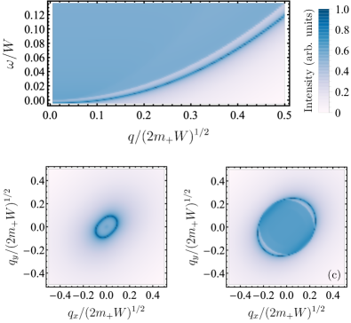
Figure 6: Pair spectral function $\mathcal{A}_{\textrm{pair}}(\mathbf{q},\omega)$ for $g=0.1$, $g_{\perp}=-0.5$, and $r_{+}=1.2$. In this case, $|g|<|g_{\perp}|$ and only one bound state appears below the two-particle continuum. Panel (a) shows $\mathcal{A}_{\textrm{pair}}(\mathbf{q},\omega)$ as a function of $q$ and $\omega$ at fixed angle $\varphi_{\mathbf{q}}=\pi/4$. Panels (b) and (c) show $\mathcal{A}_{\textrm{pair}}(\mathbf{q},\omega)$ as a function of momentum at fixed $\omega=0$ and $\omega=0.03W$, respectively.

For $q\to 0$, the result simplifies as $C(x)\sim x\to 0$ and the angle-dependent terms in Eq. (27) vanish. In this case, $X_{\pm}(\mathbf{q}=0,E_{bs}^{\pm})=(1+r_{+})/(g\mp|g_{\perp}|)$ become constant. The bound state solutions at $\mathbf{q}=0$, with energies

$$E^{\pm}_{bs}(\mathbf{q}=0)=\frac{W}{1-\exp\left(-\frac{1+r_{+}}{g\mp|g_{\perp}|}\right)}<0,$$ (29)

exist as long as $g\pm g_{\perp}<0$. Therefore, the criterion for the number of bound states at $\mathbf{q}=0$ matches the three regions depicted in Fig. 4. For $g>|g_{\perp}|$, corresponding to the regime of marginally irrelevant interactions, there are no bound states. We find one bound state with energy $E_{bs}^{+}$ in the crossover regime $|g|<|g_{\perp}|$ and two bound states in the attraction-dominated regime $g<-|g_{\perp}|$. For $g<0$ and $g_{\perp}=0$, the bound states are degenerate at $\mathbf{q}=0$. Note also that at weak coupling, $|g|,|g_{\perp}|\ll 1$, the binding energies $E^{\pm}_{bs}(0)\approx-W\exp\left(\frac{1+r_{+}}{g\mp|g_{\perp}|}\right)$ are exponentially small, as expected for marginal interactions.

For $g_{\perp}\neq 0$ and $g<-|g_{\perp}|$, the bound states may become degenerate at nonzero momenta $\mathbf{q}_{0}$ such that $X_{+}(\mathbf{q}_{0},E_{bs})=X_{-}(\mathbf{q}_{0},E_{bs})$. From Eqs. (26) and (27), we see that the degeneracy point happens along the directions where $\sin(2\varphi_{\mathbf{q}_{0}})=\textrm{sgn}(g_{\perp})$, i.e., for angles $\varphi_{\mathbf{q}_{0}}=\frac{\pi}{4},\frac{5\pi}{4}$ for $g_{\perp}>0$ and $\varphi_{\mathbf{q}_{0}}=\frac{3\pi}{4},\frac{7\pi}{4}$ for $g_{\perp}<0$. The value of $q_{0}$ is determined by the conditions

$$E_{bs}(q_{0}) = \frac{\Omega(q_{0})}{1-e^{\frac{(1+r_{+})g}{g^{2}-g_{\perp}^{2}}}}+\frac{W}{1-e^{-\frac{(1+r_{+})g}{g^{2}-g_{\perp}^{2}}}},$$ (30)

$$C\left(\frac{q_{0}^{2}/(2M)}{-E_{bs}(q_{0})}\right) = \frac{(1+r_{+})|g_{\perp}|}{g^{2}-g_{\perp}^{2}}.$$ (31)

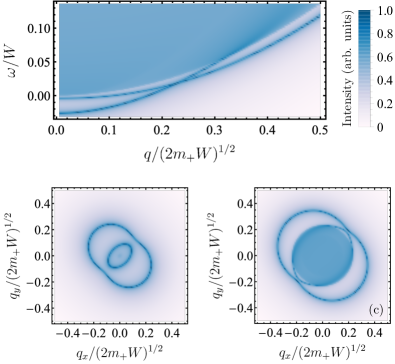
Figure 7: Same as Fig. 6 for $g=-0.5$, $g_{\perp}=0.1$, and $r_{+}=1.2$. In this case, $g<-|g_{\perp}|$ and there are two bound states below the continuum at $\mathbf{q}=0$. Note the touching of curves in panel (a), which is due to the degeneracy of the bound states with momentum $\mathbf{q}_{0}\neq 0$ along the direction $\varphi_{\mathbf{q}}=\pi/4$.

Figures 6 and 7 show results for the pair spectral function in the ladder approximation. The intensities are plotted in logarithmic scale and arbitrary units proportional to $\ln[1+A_{\textrm{pair}}(\mathbf{q},\omega)/(\eta m_{+})]$, with a small broadening factor $\eta\sim 10^{-4}$. Figure 6 is representative of the crossover regime with $|g|<|g_{\perp}|$. Although the $s$-wave scattering amplitude $g>0$ is repulsive in this example, we do find a bound state below the two-particle continuum. This bound state originates from the effects of anisotropic exchange interaction encoded in $g_{\perp}$. On the other hand, in the attraction-dominated regime $g<-|g_{\perp}|$ illustrated by Fig. 7, we find two bound states at $\mathbf{q}=0$. These bound states become degenerate at a finite value of $q$ in the direction $\varphi_{\mathbf{q}}=\pi/4$, see the anticrossing in Fig. 7(a). This dependence on $\varphi_{\mathbf{q}}$ is a manifestation of the unitary transformation in Eq. (17), which is responsible for the nontrivial Berry phase of the QBT point. Note that the bound state dispersions only exhibit a C₂ rotational symmetry, consistent with the anisotropy of the dipolar exchange interaction in the lattice model. This contrasts with the isotropic single-fermion and impurity dispersions, which account for the rotational invariance of the edge of two-particle continuum seen in Figs. 6 and 7.

Figure 8: A-sublattice component $\mathcal{A}^{A}_{\textrm{pair}}(\mathbf{q},\omega)$ of the pair spectral function for $g=-0.5$, $g_{\perp}=0$, and $r_{+}=1.2$. Panel (a) shows the result as a function of $q$ and $\omega$ at fixed $\varphi_{\mathbf{q}}=\pi/4$. The two bound states become degenerate as $q\to 0$. Panels (b) and (c), taken at fixed $\omega=0$ and $\omega=0.02W$, respectively, show that the first (second) bound state has vanishing weight in the A sublattice for $\varphi_{\mathbf{q}}=0,\pi$ ($\varphi_{\mathbf{q}}=\pi/2,3\pi/2$). The angle dependence of the B-sublattice component can be obtained by a C₄ rotation of plots (b) and (c).

Finally, consider the case $g<0$ and $g_{\perp}=0$, which holds for the standard attractive Fermi Hubbard model without the dipolar exchange interaction. In this case, we are left with the rotationally invariant $g$ interaction. Nevertheless, the bound states can still show signatures of the $d$-wave character of the QBT. Figure 8 displays the A-sublattice component of the pair spectral function, defined as $\mathcal{A}^{A}_{\textrm{pair}}(\mathbf{q},\omega)=-2\textrm{Im}\{\Pi_{AA}(\mathbf{q},\omega+i0^{+})\}$. In Fig. 8(a), we see that the two bound states are degenerate at $\mathbf{q}=0$, but the degeneracy is lifted as $q$ increases and the second bound state eventually merges with the continuum. Moreover, figures 8(b) and 8(c) show that the bound state contributions to $\mathcal{A}^{A}_{\textrm{pair}}(\mathbf{q},\omega)$ have nodes as a function of $\varphi_{\mathbf{q}}$. The weight of the first bound state in the A sublattice vanishes for $\varphi_{\mathbf{q}}=0,\pi$, while for the second bound state it vanishes for $\varphi_{\mathbf{q}}=\pi/2,3\pi/2$. Along these four directions, $\mathcal{A}^{A}_{\textrm{pair}}(\mathbf{q},\omega)$ shows only one bound state below the continuum at small $q$. The location of the nodes is reversed for the B-sublattice component of the pair spectral function. If we add A and B components, we find that the full pair spectral function is symmetric under C₄ rotations, with two bound states in any direction for small $q$. To gain more intuition about the symmetry properties of the bound states, in Appendix B we study the two-body problem of an impurity interacting with a single particle near the QBT point, without the constraint of a completely filled lower band.

V Conclusion

We studied the interaction between a mobile quantum impurity and a bath of majority fermions whose Fermi level is tuned to a quadratic band touching point. The low-energy effective model contains an $s$-wave contact interaction $g$ and a rotational-symmetry-breaking interaction $g_{\perp}$ which can be generated by dipolar spin exchange. A renormalization group approach shows a regime in which a repulsive impurity-fermion interaction becomes effectively attractive at low energies. This happens because the dipolar spin exchange switches the fermion and the impurity positions, lowering the ground state energy. The amplitude of this process decreases with distance. This situation leads to the formation of bound states. The anisotropic momentum dependence of the bound states stems from the combined effects of the $g_{\perp}$ interaction and the $d$-wave terms in the two-particle propagator. In the ladder approximation, we find a single bound state for $|g|<|g_{\perp}|$ and two bound states for $g<-|g_{\perp}|$, in agreement with the existence of different regimes in the renormalization group flow diagram. At weak coupling, the binding energies are exponentially small in the coupling constants.

Higher body bound states, as trimers or tetramers, are not expected to have important contribution to the spectral functions discussed in this work, unless one considers the impurity to be substantially lighter than the fermions and considers the regime of strong interactions, where $p$-wave interactions between the fermions could develop. In addition, the presence of a Fermi sea usually tends to suppress the formation of higher body bound states due to the Pauli exclusion principle, requiring the impurity to be even lighter to allow those bound states Naidon and Endo (2017). Our model could be realized with dipolar molecules in an optical checkerboard lattice. It should be interesting to extend our results to a low but finite density of minority fermions, with potential implications for unconventional superconductivity in quadratic band touching systems Pawlak et al. (2015).

Appendix A Functions

In this appendix we write down the expression for the functions $F_{i}(r_{+},r_{-})$, with $i=1,\dots,4$, that appear in the RG equations (18). These are given by

$$F_{1} = \int_{0}^{\pi/2}d\alpha\frac{(1+r_{+}^{-1})(1+r_{-}^{-1})}{\sin{\alpha}\cos{\alpha}}$$ (32)

$$\times\Bigg{[}-1+\frac{L}{\left(L^{2}-\sin^{2}(2\alpha)\right)^{1/2}}\Bigg{]},$$

$$F_{2} = \frac{1}{4}\int_{0}^{\pi/2}d\alpha\,(1+r_{+}^{-1})(1+r_{-}^{-1})\sin(2\alpha)$$ (33)

$$\times\left[-1+\frac{4L}{\left(L^{2}-\sin^{2}(2\alpha)\right)^{3/2}}\right],$$

$$F_{3} = 2\int_{0}^{\pi/2}d\alpha\frac{[(1+r_{+}^{-1})(1+r_{-}^{-1})]^{3/2}}{(L^{2}-\sin^{2}{(2\alpha)})^{3/2}}$$ (34)

$$\times\Big{\{}(1-3L)\sin{(2\alpha)}$$

$$\left.\qquad+\frac{2\big{[}(L^{2}-\sin^{2}{(2\alpha)})^{3/2}-L^{3}\big{]}}{\sin{(2\alpha)}}\right\},$$

$$F_{4} = \int_{0}^{\pi/2}d\alpha\frac{[(1+r_{+}^{-1})(1+r_{-}^{-1})]^{3/2}}{(L^{2}-\sin^{2}{(2\alpha)})^{5/2}}\sin{(2\alpha)}$$ (35)

$$\times\big{[}(1-3L)\sin^{2}{(2\alpha)}+2L^{2}\big{]},$$

where

$$L(\alpha) = (1+r_{-}^{-1})\cos^{2}{\alpha}+(1+r_{+}^{-1})\sin^{2}{\alpha}.$$ (36)

Appendix B Two-body problem

In this appendix we consider the two-body problem described by the Schrödinger equation

$$E\Phi(\mathbf{r}_{1},\mathbf{r}_{2}) = \left[h_{0}(\mathbf{r}_{1})-\frac{\openone}{2M}\nabla_{\mathbf{r}_{2}}^{2}\right]\Phi(\mathbf{r}_{1},\mathbf{r}_{2})$$ (37)

$$+\delta(\mathbf{r}_{1}-\mathbf{r}_{2})(g\openone+g_{\perp}\sigma^{x})\Phi(\mathbf{r}_{1},\mathbf{r}_{2}),$$

where $\Phi(\mathbf{r}_{1},\mathbf{r}_{2})$ is the wave function with the first particle representing the fermion near the QBT and the second particle representing the impurity. In addition to the dependence on the coordinates $\mathbf{r}_{1}$ and $\mathbf{r}_{2}$, the wave function contains a spinor in sublattice space for the first particle. Taking the Fourier transform of Eq. (37), we obtain

$$E\tilde{\Phi}(\mathbf{p}_{1},\mathbf{p}_{2}) = \left[h_{0}(\mathbf{p}_{1})+\openone\frac{p^{2}_{2}}{2M}\right]\tilde{\Phi}(\mathbf{p}_{1},\mathbf{p}_{2})$$

$$+\int\frac{d^{2}q}{(2\pi)^{2}}(g\openone+g_{\perp}\sigma^{x})\tilde{\Phi}(\mathbf{p}_{1}+\mathbf{q},\mathbf{p}_{2}-\mathbf{q}).$$

Let us focus on the case $\mathbf{P}=\mathbf{p}_{1}+\mathbf{p}_{2}=0$, corresponding to vanishing center-of-mass momentum. We then define

$$\Delta(\mathbf{p})=\left[\left(E-\frac{p^{2}}{2M}\right)\openone-h_{0}(\mathbf{p})\right]\tilde{\Phi}(\mathbf{p},-\mathbf{p}),$$ (39)

and obtain

$$\Delta(\mathbf{p}) = \int\frac{d^{2}q}{(2\pi)^{2}}(g\openone+g_{\perp}\sigma^{x})$$ (40)

$$\times\left[\left(E-\frac{q^{2}}{2M}\right)\openone-h_{0}(\mathbf{q})\right]^{-1}\Delta(\mathbf{q}).$$

Since the right-hand side of Eq. (40) does not depend on $\mathbf{p}$, we have that $\Delta(\mathbf{p})=\Delta_{0}$ is a constant spinor. Thus, Eq. (40) reduces to the eigenvalue equation

$$\mathcal{R}\Delta_{0}=\Delta_{0},$$ (41)

where

$$\mathcal{R} = \int\frac{d^{2}q}{(2\pi)^{2}}(g\openone+g_{\perp}\sigma^{x})$$ (42)

$$\times\left[\left(E-\frac{q^{2}}{2M}\right)\openone-h_{0}(\mathbf{q})\right]^{-1}.$$

To solve Eq. (42), we use the unitary transformation that diagonalizes $h_{0}(\mathbf{q})$ and perform the integral in the disc $0<q<(2m_{+}W)^{1/2}$ with high-energy cutoff $W$. We find that bound state solutions with $E=\mathcal{E}_{bs}<0$ exist only if $m_{-}>M$. This condition is not satisfied for the lattice model discussed in Sec. II, but more generally one could modify the band structure by adding further hopping processes or make the impurity out of another atomic species with a different mass. At weak coupling, the binding energies scale as

$$\mathcal{E}^{\pm}_{bs}\sim-W\exp\left[\frac{m_{+}}{(\bar{\mu}_{+}+\bar{\mu}_{-})(g\pm g_{\perp})}\right],$$ (43)

where $\bar{\mu}_{+}=\mu_{+}$ and $\bar{\mu}_{-}=m_{-}M/(m_{-}-M)$. The bound states are degenerate for $g_{\perp}=0$. If $g_{\perp}\neq 0$, there is no bound state for $g>|g_{\perp}|$, one bound state for $|g|<|g_{\perp}|$ and two bound states for $g<-|g_{\perp}|$. This result is equivalent to the criterion for bound states in the many-body problem.

We obtain the bound state wave functions for $\mathbf{P}=0$ by substituting the eigenvectors $\Delta_{0}$ from Eq. (41) into Eq. (39). In the regime where the bound states exist, we have

$$\tilde{\Phi}_{\pm}(\mathbf{p},-\mathbf{p}) = \mathcal{N}\Big{\{}f_{s}(p,\mathcal{E}_{bs}^{\pm})\openone+f_{d}(p,\mathcal{E}_{bs}^{\pm})\left[\cos(2\varphi_{\mathbf{p}})\sigma^{z}\right.$$ (46)

$$\left.+\sin(2\varphi_{\mathbf{p}})\sigma^{x}\right]\Big{\}}\left(\begin{array}[]{c}1\\ \pm 1\end{array}\right),$$

where $\mathcal{N}$ is a normalization factor. The functions

$$f_{s}(p,\mathcal{E}) = \left(\frac{p^{2}}{2\bar{\mu}_{+}}-\mathcal{E}\right)^{-1}+\left(\frac{p^{2}}{2\bar{\mu}_{-}}-\mathcal{E}\right)^{-1},$$

$$f_{d}(p,\mathcal{E}) = \left(\frac{p^{2}}{2\bar{\mu}_{+}}-\mathcal{E}\right)^{-1}-\left(\frac{p^{2}}{2\bar{\mu}_{-}}-\mathcal{E}\right)^{-1},$$ (47)

represent the amplitudes of the $s$- and $d$-wave components of the bound state wave function, respectively. Note that $f_{d}(p,\mathcal{E})$ vanishes for $p\to 0$. At nonzero $p$, we can write $\tilde{\Phi}_{\pm}(\mathbf{p},-\mathbf{p})=\chi_{\pm}(p,\varphi_{\mathbf{p}})$, with the symmetry properties

$$\chi_{\pm}\left(p,\varphi_{\mathbf{p}}+\frac{\pi}{4}\right) = \pm\sigma^{x}\chi_{\pm}\left(p,-\varphi_{\mathbf{p}}+\frac{\pi}{4}\right),$$

$$\chi_{\pm}\left(p,\varphi_{\mathbf{p}}-\frac{\pi}{4}\right) = \pm\sigma^{x}\chi_{\pm}\left(p,-\varphi_{\mathbf{p}}-\frac{\pi}{4}\right).$$ (48)

For $g_{\perp}=0$, the bound states become degenerate, $\mathcal{E}_{bs}^{+}=\mathcal{E}_{bs}^{-}$, and we have

$$i\sigma^{y}\chi_{\pm}\left(p,\varphi_{\mathbf{p}}+\frac{\pi}{2}\right)=\pm\chi_{\mp}(p,\varphi_{\mathbf{p}}).$$ (49)

In this case we can take linear combinations of $\chi_{+}(p,\varphi_{\mathbf{p}})$ and $\chi_{-}(p,\varphi_{\mathbf{p}})$ to form eigenstates of the C₄ rotation.

Both $s$- and $d$-wave components in Eq. (47) have a Lorentzian dependence on $p$. This implies an exponential decay as a function of the relative distance $r=|\mathbf{r}_{1}-\mathbf{r}_{2}|$ in real space, with length scales $\sim(\bar{\mu}_{\pm}|\mathcal{E}_{bs}|)^{-1/2}$.

References

- Fradkin (2013) E. Fradkin, Field Theories of Condensed Matter Physics (Cambridge University Press, 2013).
- Sun et al. (2009) K. Sun, H. Yao, E. Fradkin, and S. A. Kivelson, Phys. Rev. Lett. 103, 046811 (2009).
- Liu et al. (2010) Q. Liu, H. Yao, and T. Ma, Phys. Rev. B 82, 045102 (2010).
- Uebelacker and Honerkamp (2011) S. Uebelacker and C. Honerkamp, Phys. Rev. B 84, 205122 (2011).
- Dóra et al. (2014) B. Dóra, I. F. Herbut, and R. Moessner, Phys. Rev. B 90, 045310 (2014).
- Sur et al. (2018) S. Sur, S.-S. Gong, K. Yang, and O. Vafek, Phys. Rev. B 98, 125144 (2018).
- Zeng et al. (2018) T.-S. Zeng, W. Zhu, and D. Sheng, npj Quantum Materials 3, 49 (2018).
- Ölschläger et al. (2012) M. Ölschläger, G. Wirth, T. Kock, and A. Hemmerich, Phys. Rev. Lett. 108, 075302 (2012).
- Sun et al. (2012) K. Sun, W. V. Liu, A. Hemmerich, and S. Das Sarma, Nat. Phys. 8, 67 (2012).
- Li and Liu (2016) X. Li and W. V. Liu, Rep. Prog. Phys. 79, 116401 (2016).
- Massignan et al. (2014) P. Massignan, M. Zaccanti, and G. M. Bruun, Rep. Prog. Phys. 77, 034401 (2014).
- Zöllner et al. (2011) S. Zöllner, G. M. Bruun, and C. J. Pethick, Phys. Rev. A 83, 021603 (2011).
- Mathy et al. (2011) C. J. M. Mathy, M. M. Parish, and D. A. Huse, Phys. Rev. Lett. 106, 166404 (2011).
- Parish (2011) M. M. Parish, Phys. Rev. A 83, 051603 (2011).
- Klawunn and Recati (2011) M. Klawunn and A. Recati, Phys. Rev. A 84, 033607 (2011).
- Schmidt et al. (2012) R. Schmidt, T. Enss, V. Pietilä, and E. Demler, Phys. Rev. A 85, 021602 (2012).
- Schirotzek et al. (2009) A. Schirotzek, C.-H. Wu, A. Sommer, and M. W. Zwierlein, Phys. Rev. Lett. 102, 230402 (2009).
- Koschorreck et al. (2012) M. Koschorreck, D. Pertot, E. Vogt, B. Frohlich, M. Feld, and M. Kohl, Nature 485, 619 (2012).
- Kohstall et al. (2012) C. Kohstall, M. Zaccanti, M. Jag, A. Trenkwalder, P. Massignan, G. M. Bruun, F. Schreck, and R. Grimm, Nature 485, 615 (2012).
- Scazza et al. (2017) F. Scazza, G. Valtolina, P. Massignan, A. Recati, A. Amico, A. Burchianti, C. Fort, M. Inguscio, M. Zaccanti, and G. Roati, Phys. Rev. Lett. 118, 083602 (2017).
- Grusdt et al. (2016) F. Grusdt, N. Y. Yao, D. Abanin, M. Fleischhauer, and E. Demler, Nat. Comm. 7, 11994 (2016).
- Camacho-Guardian et al. (2019) A. Camacho-Guardian, N. Goldman, P. Massignan, and G. M. Bruun, Phys. Rev. B 99, 081105 (2019).
- Qin et al. (2019) F. Qin, X. Cui, and W. Yi, Phys. Rev. A 99, 033613 (2019).
- Grusdt et al. (2019) F. Grusdt, N. Y. Yao, and E. A. Demler, Phys. Rev. B 100, 075126 (2019).
- Caracanhas et al. (2013) M. A. Caracanhas, V. S. Bagnato, and R. G. Pereira, Phys. Rev. Lett. 111, 115304 (2013).
- Punk and Sachdev (2013) M. Punk and S. Sachdev, Phys. Rev. A 87, 033618 (2013).
- Caracanhas and Pereira (2016) M. A. Caracanhas and R. G. Pereira, Phys. Rev. B 94, 220302 (2016).
- Yan et al. (2019) Z. Z. Yan, Y. Ni, C. Robens, and M. W. Zwierlein, (2019), arXiv:1904.02685 .
- Lahaye et al. (2009) T. Lahaye, C. Menotti, L. Santos, M. Lewenstein, and T. Pfau, Rep. Prog. Phys. 72, 126401 (2009).
- Yan et al. (2013) B. Yan, S. A. Moses, B. Gadway, J. P. Covey, K. R. A. Hazzard, A. M. Rey, D. S. Jin, and J. Ye, Nature 501, 521 (2013).
- Hazzard et al. (2014) K. R. A. Hazzard, B. Gadway, M. Foss-Feig, B. Yan, S. A. Moses, J. P. Covey, N. Y. Yao, M. D. Lukin, J. Ye, D. S. Jin, and A. M. Rey, Phys. Rev. Lett. 113, 195302 (2014).
- Gorshkov et al. (2011) A. V. Gorshkov, S. R. Manmana, G. Chen, J. Ye, E. Demler, M. D. Lukin, and A. M. Rey, Phys. Rev. Lett. 107, 115301 (2011).
- Zou et al. (2017) H. Zou, E. Zhao, and W. V. Liu, Phys. Rev. Lett. 119, 050401 (2017).
- Murray and Vafek (2014) J. M. Murray and O. Vafek, Phys. Rev. B 89, 201110 (2014).
- Shankar (1994) R. Shankar, Rev. Mod. Phys. 66, 129 (1994).
- Cardy et al. (1996) J. Cardy, P. Goddard, and J. Yeomans, Scaling and Renormalization in Statistical Physics (Cambridge University Press, 1996).
- Mahan (2000) G. Mahan, Many-Particle Physics (Springer, 2000).
- Naidon and Endo (2017) P. Naidon and S. Endo, Reports on Progress in Physics 80, 056001 (2017).
- Pawlak et al. (2015) K. A. Pawlak, J. M. Murray, and O. Vafek, Phys. Rev. B 91, 134509 (2015).